Image Tag Refinement by Regularized Latent Dirichlet Allocation

Abstract

Tagging is nowadays the most prevalent and practical way to make images searchable. However, in reality many manually-assigned tags are irrelevant to image content and hence are not reliable for applications. A lot of recent efforts have been conducted to refine image tags. In this paper, we propose to do tag refinement from the angle of topic modeling and present a novel graphical model, regularized Latent Dirichlet Allocation (rLDA). In the proposed approach, tag similarity and tag relevance are jointly estimated in an iterative manner, so that they can benefit from each other, and the multi-wise relationships among tags are explored. Moreover, both the statistics of tags and visual affinities of images in the corpus are explored to help topic modeling. We also analyze the superiority of our approach from the deep structure perspective. The experiments on tag ranking and image retrieval demonstrate the advantages of the proposed method.

url]http://research.microsoft.com/en-us/um/people/jingdw/

1 Introduction

The community-contributed multimedia content in the internet, such as Flickr, Picasa, Youtube and so on, has been exploding. To facilitate the organization of the uploaded images or videos, media repositories usually offer a tool to enable consumers to manually assign tags (a.k.a. labels) to describe the media content [1]. These assigned tags are adopted to index the images to help consumers access shared media content.

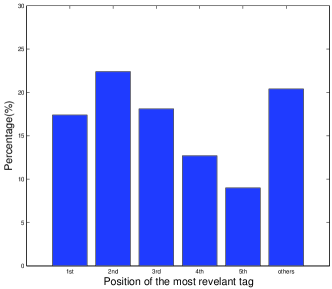
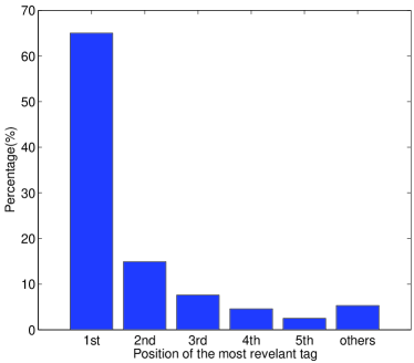
Reliable tagging results in making shared media more easily accessible to the public. However, the reliability of tagging is not guaranteed in that the tags may be noisy, orderless and incomplete [17], possibly due to carelessness of the taggers. First, some tags are noises and may be irrelevant to media. According to the statistics in Flickr, there are about only $50\%$ tags indeed relevant to photos [17, 10]. Second, different tags essentially have different relevance degrees to the media, but such information is not indicated in the current tag list, where the order is given according to the input sequence. We did an analysis on the MSRA-TAG dataset [24], which was crawled from Flickr, about what percentage of images have the most important tags in different positions. A statistics figure is shown in Fig.1 to indicate the result. It can be observed from this statistics that less than $20\%$ images have the most relevant tags at the top position, which shows that the tags are almost in a random order in terms of the relevance. Last, the tags of some photos are incomplete due to the interest limitation of taggers, and even not given.

Figure 1: A statistic on the MSRA-TAG dataset [24] indicating the percentage of images with the most relevant tag in different positions.

We address the problem of refining the tags, to facilitate the access of the shared media. To be specific, we investigate the tagging problem in Flickr, one of the most popular photo sharing web sites, and propose to reorder the tags. The available information to refine the tags consists of manual tags and image affinity.

1. Although they are not completely reliable, the manual tags still reflect the photo content in some degree and their relations can be explored for tag refinement. Existing solutions only make use of the pairwise relation between tags, mined from WordNet [31], or estimated from Web photo tags [21, 22, 24, 35].

2. Visually similar images usually tend to have similar semantics and hence have similar tags, which means that the tag refinement of one image may benefit from those of other images. The typical exploration [24, 22] is to utilize the visual popularity of one image among the images having the same tag as a cue to estimate the relevance of the tag with this image.

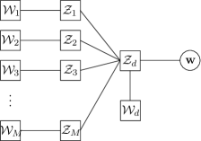
In this paper, we present a novel probabilistic formulation, to estimate the relevance of a tag by considering all the other images and their tags. To this goal, we propose a novel model called regularized latent Dirichlet allocation (rLDA), which estimates the latent topics for each document, with making use of other documents. The model is applicable in tag refinement due to the observation that the content of an image essentially contains a few topics and the reasonable assumption that the tags assigned to the image accordingly form a few groups. The latent topics are estimated by viewing the tags of each image as a document, and the estimation also benefits from other visually similar images by the regularization term, instead of the estimation by LDA only from the corresponding document. The main contribution of our approach lies in the following aspects. On the one hand, both LDA and rLDA explore the multiple-wise relation among tags through the latent topics, rather than pairwise relations in the random walk based methods. On the other hand, the tag relevance estimation from rLDA can be interpreted using the deep structure [3, 13]. Compared with random walk and LDA, our approach is the deepest, and the illustration is presented in Figure 2.

2 Related work

The automatic image tagging or annotation problem is usually regarded as an image classification task. Typical techniques [2, 4, 7, 9, 11, 12, 14, 16, 20, 28, 29, 33] usually learn a generative/discriminative multi-class classifier from the training data, to construct a mapping function from low level features extracted from the images to tags, and then predict the annotations or tags for the test images. Later, a more precise formulation is presented to regard it as a multi-label classification problem by exploring the relations between multiple labels [15, 30]. The automatic annotation techniques have shown great successes with small scale tags and the well-labeled training data. But in the social tags, e.g., image tags on Flickr, there exist noisy or low-relevance tags, and the vocabulary of tags is very large, which limits the performance of conventional automatic tagging techniques in social tagging. The study in [17] has shown that classifiers trained with Flickr images and associated tags got unsatisfactory performance and that tags provided by Flickr users actually contain noise. Moreover, the relevance degrees of the tags, i.e., the order of the tags, are not investigated in automatic annotation.

Various approaches have been developed to refine tags using the available tags and visual information. The following reviews some closely-related methods, and more discussions can be found from a survey [34]. The straightforward approach directly exploits the tag relation, e.g., co-occurrence relation mined from WordNet [26], or the internet, and then refines tags [31, 35, 19]. For example, the tag ambiguities are resolved [35] by finding two tags that appear in different contexts but are both likely to co-occur with the original tag set and then presenting such ambiguous tags to users for further clarification. The random walk approach over the pairwise graph on the provided tags with edges weighted by the tag similarities is presented in [32, 24]. The visual information is proved very useful to help tag refinement. For example, the neighborhood voting approach [21] is to recommend the tags by exploring the tags of the visually similar images. The likelihood that a tag is associated with an image is computed in [32, 24] from probabilistic models learnt the images assigned with such a tag, and then put it into the random walk framework for further refinement. A hybrid probabilistic model [38] is introduced to combine both collaborative and content based algorithms for tagging, which is similar to [24] in using the visual contents. A RankBoost based approach [36] is presented to learn a function to combine ranking features from multi-modalities, including tag and visual information. An optimization framework [23] is proposed to perform tag filter and enrichment by exploring visual similarity and additional knowledge from WordNet [26]. An approach [39] formulates the tag refinement problem as a decomposition of the user-provided tag matrix into a low-rank matrix and a sparse error matrix, targeting the optimality by low-rank, content consistency, tag correlation and error sparsity.

Rather than exploring the pairwise relation among tags, some techniques are proposed to adopt the multiple wise relations among tags, through latent models. Latent topic models, alternatives of latent Dirichlet allocation, is adopted [19, 18, 6] to learn a generative model from the tags, which then can estimate the posterior probability that a tag is associated with an image. Those methods are limited in lack of capabilities of adopting visual information. Therefore, this paper proposes a novel topic model, called regularized latent Dirichlet allocation, to estimate the topic models with exploiting the visual information. The latent topic based models are also justified by the conclusion in [31] that these tags assigned to images span a broad spectrum of the semantic space.

From the perspective of the deep learning theory [13], the random walk based approaches essentially estimate the tag relevance with a shallow structure, which only consists of two levels, the provided tags as the input level and the tag being considered as the output level. The LDA based approach is with a deep structure, introducing a latent topic level, which has potential to get better performance. The proposed regularized LDA model is deeper, with four levels, the tags associated with other images as the first level, the latent topics of other images and the tags of the image being considered as the second level, the latent topic as the third level, and the tag being considered as the output level.

The relational topic model [8] is closely related to the proposed regularized LDA. But they are clearly different because our approach imposes the regularization over the topic distribution instead of the latent variables and moreover our approach deals multiple modalities and makes use of additional visual similarity to formulate the regularization term. Our approach is also different from topic models for image annotation [4, 2, 28, 29]: The image tagging problem in our paper is more challenging than image annotation as aforementioned. and moreover the proposed regularized LDA aims to impose the consistency of tags within similar images while they are supervised algorithms [28, 29] or aim to find common topics shared by tags and visual contents. This paper is different from the short version [37] because we present a formal derivation of our approach, introduce a new inference approach conduct more experiments, and particularly, we use the deep network structure to analyze the benefit of regularized LDA.

(a) (a)

(b) (b)

(c) (c)

Figure 2: Illustration from the graphical representations. (a) Two layers for pairwise based approaches. (b) Three layers for LDA. (c) Four layers for our approach (rLDA). It can be concluded that our approach is deeper.

3 Taxonomy

The input consists of an image corpus, $M$ images $\mathcal{I}=\{I_{1},\cdots,I_{M}\}$, and $M$ tag documents $\mathcal{W}=\{\mathcal{W}_{1},\cdots,\mathcal{W}_{M}\}$, with $\mathcal{W}_{k}$ being the set of tags manually assigned to image $I_{k}$. Here $\mathcal{W}_{k}$ is defined, similarly to [5], as a sequence of $N_{k}$ words denoted by $\mathcal{W}_{k}=\{\mathbf{w}_{1},\mathbf{w}_{2},\cdots,\mathbf{w}_{N_{k}}\}$. $\mathbf{w}_{i}$ represents a word, an item from a vocabulary indexed by $\{1,\cdots,V\}$, and is a $V$-dimensional vector, with only one entry equal to 1 and all the other entries equal to 0, e.g., $w^{v}_{i}=1$ and $w^{u}_{i}=0$ for $u\neq v$ if $\mathbf{w}_{i}$ represents the $v$-th word. Besides, we use $\mathbf{f}_{k}$ to represent the visual feature of image $I_{k}$. The goal is to reorder the tags in each document, finding reordered tags $\{\mathbf{w}_{n_{1}},\mathbf{w}_{n_{2}},\cdots,\mathbf{w}_{n_{N_{k}}}\}$ with $\{n_{1},n_{2},\cdots,n_{N_{k}}\}$ being a permutation of $\{1,2,\cdots,N_{k}\}$, so that the tags on the top are semantically more relevant to the image.

Given the image corpus and the associated tag documents, we introduce a term, tag relevance, which is then used to reorder the tags. The tag relevance is inferred based on the joint probability, $P(\mathcal{W}_{1},\cdots,\mathcal{W}_{d},\cdots,\mathcal{W}_{M}|I_{1},\cdots,I_{d},\cdots,I_{M})$.

3.1 Formulation with the tag cue

The manually-assigned tags, in some degree, describe the semantic content of an image, although it may contain noise, or not be complete. Hence, as a candidate solution, the relevance of each tag can be inferred from these tags. The joint probability over the tags $\mathcal{W}_{d}$ of image $I_{d}$ is formulated as a pairwise Markov random field (MRF),

$$P(\mathcal{W}_{d})\propto\prod_{i,j\in\{1,\cdots,N_{d}\}}P(\mathbf{w}_{di},\mathbf{w}_{dj}),$$ (1)

where $P(\mathbf{w}_{di},\mathbf{w}_{dj})$ is valuated from the tag relation. This model can be further interpreted by a random walk model. Specifically, a transition probability is defined from the tag relation as

$$T_{\mathbf{w}_{di}\rightarrow\mathbf{w}_{dj}}\propto\text{sim}(\mathbf{w}_{di},\mathbf{w}_{dj}).$$ (2)

Here $T_{\mathbf{w}_{di}\rightarrow\mathbf{w}_{dj}}$ has been normalized such that $\sum_{j\in\{1,\cdots,N_{d}\}}T_{\mathbf{w}_{di}\rightarrow\mathbf{w}_{dj}}=1$. $\text{sim}(\mathbf{w}_{di},\mathbf{w}_{dj})$ is the similarity between $\mathbf{w}_{di}$ and $\mathbf{w}_{dj}$, and may be computed from WordNet [31] or other methods [21, 22, 24, 35]. Given this model, the stable distribution of this model, $\mathbf{p}^{s}=[P(\mathbf{w}_{d1})~{}\cdots~{}P(\mathbf{w}_{dN_{d}})]$ is then used to evaluate the relevance of each tag.

3.2 Formulation with the visual cue

The visual description of a tag, $u$, can be obtained from a set of images, $\mathcal{I}_{u}=\{I_{k}|u\in\mathcal{W}_{k}\}$, associated with that tag. Given an image $I$, the posteriori probability $p(u|I)$ can be computed as follows,

$$p(u|I)=\frac{p(I|u)p(u)}{p(I)}\propto p(I|u)p(u),$$ (3)

where $p(I|u)$ can be estimated by $p(I|u)=p(I|\mathcal{I}_{u})$ that can be computed using the kernel density estimation [24], e.g., $p(I|u)\propto\sum_{I^{\prime}\in\mathcal{I}_{u}}K(I,I^{\prime})$. The scheme estimating the density can also be interpreted as the stable distribution of a random walk over the images $\mathcal{I}_{u}$, where the transition probability is estimated from the kernel $K(I,I^{\prime})$. Without any bias for any tag, $p(u)$ can be thought as a uniform distribution. To the end, $p(u|I)\propto p(I|u)$ can be used as the relevance of tag $u$ for image $I$.

3.3 Formulation with both tag and visual cues

As a straightforward scheme exploring of both tag and visual cues, the relevances from the visual cue can be viewed as observations to the probability model over tags. Denote $p_{v}(\mathbf{w}_{di})$ as the observations of tag $\mathbf{w}_{di}$, the model can be written as

$$P(\mathcal{W}_{d})\propto\prod_{i}p_{v}(\mathbf{w}_{di})\prod_{i,j\in\{1,\cdots,N_{d}\}}P(\mathbf{w}_{di},\mathbf{w}_{dj}).$$ (4)

It can also be interpreted as a random walk with restarts. The transition model is the same to Eqn. (2), and $p_{v}(\mathbf{w}_{di})$, first normalized so that $\sum_{i\in\{1,\cdots,N_{d}\}}p_{v}(\mathbf{w}_{di})=1$, is viewed as the restarts. The resulted approach includes two steps: relevance from visual cue and a random walk with restart over tags. The solution is essentially the fixed point $\mathbf{p}^{s}=\lambda\mathbf{T}^{T}\mathbf{p}^{s}+(1-\lambda)\mathbf{p}^{v}$, where $\mathbf{p}^{v}=[p_{v}(\mathbf{w}_{d1})\cdots p_{v}(\mathbf{w}_{dN_{d}})]$. The two-step approach, presented in [24], can be cast into this formulation.

3.4 Extension to a joint formulation

The above formulations actually consider each image independently, and as a result, tag relevances for each image can be estimated separately. In the computation of $p(I|u)=p(I|\mathcal{I}_{u})$, each image in the set, $\mathcal{I}_{u}=\{I_{k}|u\in\mathcal{W}_{k}\}$, is equivalently considered. In fact, an image is associated with several tags, and accordingly the typicality degree of each image to represent the tag may be different. Alternatively, the tag relevance can be jointly estimated by considering a joint probability,

$$P(\mathcal{W}_{1},\cdots,\mathcal{W}_{d},\cdots,\mathcal{W}_{M})$$

$$\propto (\prod_{d}\prod_{u,v\in\{1,\cdots,N_{d}\}}P(\mathbf{w}_{du},\mathbf{w}_{dv}))(\prod_{d}\prod_{u}p(I_{d}|u)),$$ (5)

where the first term corresponds to the pairwise MRF, and the second term is from the visual constraint and can be viewed as the visual regularization. $p(I|u)$, can be furthermore written as $p(I|u)=p(I|\mathcal{I}_{u},\mathcal{A}_{u})\propto\sum_{I^{\prime}\in\mathcal{I}_{u}}a_{u}(I^{\prime})K(I,I^{\prime})$, (viewed as a weighted random walk model) where $\mathcal{A}_{u}=\{a_{u}(I^{\prime})|I^{\prime}\in\mathcal{I}_{u}\}$ is a set of weights, with each corresponding to the typicality degree of each image and estimated as $P(I|u)$. To the end, the solution of the approach can be equivalently obtained by solving a fixed point problem,

$$\mathbf{p}^{s}_{d\cdot} =\lambda\mathbf{T}_{d}^{T}\mathbf{p}^{s}_{d\cdot}+(1-\lambda)\mathbf{p}^{o}_{d\cdot},$$ (6)

$$\bar{\mathbf{p}}^{o}_{\cdot u} =\mathbf{T}^{w}_{u}\bar{\mathbf{p}}^{o}_{\cdot u},$$ (7)

where $\mathbf{T}^{w}_{u}\propto\operatorname{diag}(\mathbf{p}^{s}_{\cdot u})\mathbf{P}$ is a weighted transition matrix, with $\mathbf{P}$ corresponding to the pairwise probability $P(\mathbf{w}_{du},\mathbf{w}_{dv})$, $\bar{\mathbf{p}}^{o}_{\cdot u}$ and $\mathbf{p}^{o}_{d\cdot}$ are the observation probability vectors, a column vector and a row vector of $\mathbf{P}=[p(I_{d}|u)]_{M\times V}$ normalized w.r.t. image set and tag set, respectively.

4 Our approach

The aforementioned approach builds the relationship among the tags, using the pairwise framework, which is lack of the ability to describe the multiple wise relations among tags. However, we observed that the relation among tags is beyond pairwise and that some tags may have closed relations and the tags associated with one image form several meaningful cliques. To make use of the multiple wise relations, we introduce a topic model to construct the tag relation, which uses latent topic variables to connect the tags for building the multiple wise relationships. Moreover, rather than separately building the topic model independently for each image, we propose a novel approach to jointly model the images together based on the observation that visually similar images should have similar semantic contents, To this goal, we introduce smoothness terms over the latent topics of images.

4.1 Tag refinement via latent Dirichlet allocation

(a) (a)

(b) (b)

Figure 3: (a) Graphical model representation of LDA. (b) Graphical model representation of the variational distribution used to approximate the posterior in LDA

4.1.1 Latent Dirichlet allocation

Latent Dirichlet allocation (LDA) is a generative probabilistic model of a corpus, e.g., a set of documents. The basic idea is that documents are represented as random mixtures over latent topics, where each topic is characterized by a distribution over tags (words), or intuitively is viewed as a group of soft (partially weighted) tags. LDA is a special directed graphical model (a.k.a. Bayesian network), and its graphical representation is shown in Figure 3(a). In this graphical model, $\mathbf{z}$ is a topic vector of length $k$, with $k$ being the number of latent topics, where it corresponds to the $i$ topic if $z^{i}=1$ and $z^{j}=0$ for $j\neq i$. $\boldsymbol{\theta}$ is a $k$-dimensional vector, the parameter of the multinomial distribution. $\boldsymbol{\alpha}$ is the Dirichlet parameter, a vector of $k$ positive reals. Matrix $\boldsymbol{\beta}$, of dimension $k\times V$, is used to parameterize the tag-topic probability, where $\beta_{ij}=p(w^{j}=1|z^{i}=1)$.

It can be interpreted as a generative process for each document $\mathcal{W}_{d}$ as follows.

1. Choose $\boldsymbol{\theta}_{d}\sim\operatorname{Dir}(\boldsymbol{\alpha})$.

2. For each of the $N_{d}$ tags $\mathbf{w}_{dn}$,

   1. Choose a topic $\mathbf{z}_{dn}\sim\operatorname{Multinomial}(\boldsymbol{\theta}_{d})$.

   2. Choose a tag $\mathbf{w}_{dn}$ from $p(\mathbf{w}_{dn}|\mathbf{z}_{dn};\boldsymbol{\beta})$, a multinomial probability conditioned on the topic $\mathbf{z}_{dn}$.

In the graphical representation, there are three levels. The parameters $\boldsymbol{\alpha}$ and $\boldsymbol{\beta}$ are corpus level parameters, assumed to be sampled once in the generative process for a single corpus. The variable $\boldsymbol{\theta}$ is a document-level (image-level) variable sampled for each document (image). Finally, the variables $\mathbf{z}_{dn}$ and $\mathbf{w}_{dn}$ are word-level (tag-level) variables, sampled once for each word in each document.

4.1.2 Topic distribution

The goal to use LDA here is to mine the latent topic distribution for a given document $\mathcal{W}_{d}$, $p(\boldsymbol{\theta}|\mathcal{W}_{d},\boldsymbol{\alpha},\boldsymbol{\beta})$. The topic distribution can be obtained by integrating out other latent variables $\mathbf{z}_{1},\cdots,\mathbf{z}_{N_{d}}$ over the posterior distribution, $p(\boldsymbol{\theta},\{\mathbf{z}_{1},\cdots,\mathbf{z}_{N_{d}}\}|\mathcal{W}_{d},\boldsymbol{\alpha},\boldsymbol{\beta})$. This distribution is intractable to compute in general. The approximate inference algorithms, e.g., Markov chain Monte Carlo and variational inference, can be used to tackle this problem. The variational inference algorithm introduces a variational distribution,

$$q(\boldsymbol{\theta},\{\mathbf{z}_{1},\cdots,\mathbf{z}_{N_{d}}\}|\boldsymbol{\gamma},\{\boldsymbol{\phi}_{1},\cdots,\boldsymbol{\phi}_{N_{d}}\})=q(\boldsymbol{\theta}|\boldsymbol{\gamma})\prod_{n=1}^{N_{d}}q(\mathbf{z}_{n}|\boldsymbol{\phi}_{n}),$$

where the Dirichlet parameter $\boldsymbol{\gamma}$ and the multinomial parameters $\{\boldsymbol{\phi}_{1},\cdots,\boldsymbol{\phi}_{N_{d}}\}$ are the free variational parameters. The variational parameters can be obtained from the following optimization problem:

$$\boldsymbol{\gamma}*,\{\boldsymbol{\phi}*_{1},\cdots,\boldsymbol{\phi}*_{N_{d}}\}$$

$$= \arg\min_{\boldsymbol{\gamma},\{\boldsymbol{\phi}_{1},\cdots,\boldsymbol{\phi}_{N_{d}}\}}$$

$$\operatorname{KL}(q(\boldsymbol{\theta},\{\mathbf{z}_{1},\cdots,\mathbf{z}_{N_{d}}\}|\boldsymbol{\gamma},\{\boldsymbol{\phi}_{1},\cdots,\boldsymbol{\phi}_{N_{d}}\})$$

$$~{}~{}~{}~{}~{}||p(\boldsymbol{\theta},\{\mathbf{z}_{1},\cdots,\mathbf{z}_{N_{d}}\}|\mathcal{W}_{d},\boldsymbol{\alpha},\boldsymbol{\beta})),$$ (8)

where $\operatorname{KL}(q(\cdot)|p(\cdot))$ is the Kullback-Leibler (KL) divergence between the variational distribution $q(\cdot)$ and the true posterior $p(\cdot)$. Figure 3(b) illustrates this variational distribution. This minimization can be achieved via an iterative fixed-point method. The update equations are as follows,

$$\phi_{ni} \propto\beta_{iv(\mathbf{w}_{n})}\exp\{\operatorname{E}_{q}[\log(\theta_{i})|\boldsymbol{\gamma}]\}$$ (9)

$$\gamma_{i} =\alpha_{i}+\sum_{n=1}^{N}\phi_{ni},$$ (10)

where $v(\mathbf{w})$ is a function that maps a vector representation of a word to an index in the vocabulary.

In the LDA model, two model parameters, $\boldsymbol{\alpha}$ and $\boldsymbol{\beta}$, can be estimated from the given corpus of documents, $\mathcal{W}$, by maximizing the following log likelihood,

$$L(\boldsymbol{\alpha},\boldsymbol{\beta})=\sum_{d=1}^{M}\log p(\mathcal{W}_{d}|\boldsymbol{\alpha},\boldsymbol{\beta}).$$ (11)

Here, $p(\mathcal{W}_{d}|\boldsymbol{\alpha},\boldsymbol{\beta})$ can be efficiently estimated by an expectation-maximization (EM) algorithm [5].

4.1.3 Tag relevance

Given this topic model, the relevance of a tag $\mathbf{w}$ for each image is formulated as the probability conditioned on the set of tags $\mathcal{W}$ associated with this image. It is mathematically formulated as

$$p(\mathbf{w}|\mathcal{W}) =\sum_{\bar{\boldsymbol{z}}}p(\mathbf{w},\bar{\boldsymbol{z}}|\mathcal{W})$$

$$=\sum_{\bar{\boldsymbol{z}}}p(\mathbf{w}|\bar{\boldsymbol{z}})p(\bar{\boldsymbol{z}}|\mathcal{W})$$

$$=\sum_{\bar{\boldsymbol{z}}}p(\mathbf{w}|\bar{\boldsymbol{z}})\int p(\bar{\boldsymbol{z}},\boldsymbol{\theta}|\mathcal{W})d\boldsymbol{\theta}$$

$$=\sum_{\bar{\boldsymbol{z}}}p(\mathbf{w}|\bar{\boldsymbol{z}})\int p(\bar{\boldsymbol{z}}|\boldsymbol{\theta})p(\boldsymbol{\theta}|\mathcal{W})d\boldsymbol{\theta}$$

$$\approx\sum_{\bar{\boldsymbol{z}}}p(\mathbf{w}|\bar{\boldsymbol{z}})\int p(\bar{\boldsymbol{z}}|\boldsymbol{\theta})q(\boldsymbol{\theta}|\boldsymbol{\gamma})d\boldsymbol{\theta}.$$ (12)

The computation of this conditional distribution can be illustrated by a graphical model shown in Figure 2(b). From the analysis, it can be observed that the relations between tags are built using the latent variables that is beyond the pairwise relation, illustrated in Figure 2(a), and can capture the group information.

4.2 Regularized latent Dirichlet allocation

In the LDA model discussed above, the distribution of topics for each image is estimated separately. However, the tags associated with one image may be incomplete and noisy. Consequently, the distribution of topics is not well estimated, which influences the relevance of tags. It is observed that visually similar images usually have the same semantic content. To utilize this property, we introduce a regularization term over the semantic content. Rather than imposing this over tags directly, we impose it over the latent topics because tags are sometimes too ambiguous for specifying a concept, while topics usually have clearly conceptual meanings.

The straightforward solution to impose the regularization over topics is a two-step sequential scheme: first estimate the distribution of topics for each image, and then to smooth the distribution by considering the distributions of visually similar images. Instead, we propose a collective inference scheme to estimate the distribution of latent topics. To this goal, we build a joint distribution over all the images, called regularized latent Dirichlet allocation (rLDA). This joint distribution is shown in Figure 4. Different from the latent Dirichlet allocation model, the topics over different images are connected by an extra regularization model, which is defined over the topics of a pair of images.

Figure 4: The graphical representation of regularized LDA.

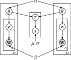
It can be interpreted as a generative process over the documents as follows.

1. For each of the $M$ documents $\mathcal{W}_{d}$

   1. Choose $\boldsymbol{\theta}_{d}\sim\operatorname{Dir}(\boldsymbol{\alpha})$.

   2. For each of the $N_{d}$ tags $\mathbf{w}_{dn}$,

      1. Choose a topic $\mathbf{z}_{dn}\sim\operatorname{Multinomial}(\boldsymbol{\theta}_{d})$.

      2. Choose a tag $\mathbf{w}_{dn}$ from $p(\mathbf{w}_{dn}|\mathbf{z}_{dn};\boldsymbol{\beta})$, a multinomial probability conditioned on the topic $\mathbf{z}_{dn}$.

2. For each of the set of document pairs $(\mathcal{W}_{d},\mathcal{W}_{d^{\prime}})$

   1. Choose $\boldsymbol{\tau}_{dd^{\prime}}\sim\operatorname{Multinomial}(\operatorname{R}(\boldsymbol{\theta}_{d},\boldsymbol{\theta}_{d^{\prime}}))$

   2. Choose a visual similarity $s_{dd^{\prime}}\sim p(\mathbf{s}_{dd^{\prime}}|\boldsymbol{\tau}_{dd^{\prime}};\boldsymbol{\mu},\boldsymbol{\sigma})$, a Gaussian probability conditioned on the latent relation topic $\boldsymbol{\tau}_{dd^{\prime}}$.

Given the parameters, $\boldsymbol{\alpha}$, $\boldsymbol{\beta}$, $\boldsymbol{\mu}$ and $\boldsymbol{\sigma}$, the joint distribution is given by

$$p(\{\boldsymbol{\theta}_{d}\},\{\{\mathbf{w}_{dn},\mathbf{z}_{dn}\}_{n}\}_{d},\{\mathbf{s}_{dd^{\prime}},\boldsymbol{\tau}_{dd^{\prime}}\}_{dd^{\prime}}|\boldsymbol{\alpha},\boldsymbol{\beta},\boldsymbol{\mu},\boldsymbol{\sigma})$$

$$= \prod_{d=1}^{M}[p(\boldsymbol{\theta}_{d}|\boldsymbol{\alpha})\prod_{i=1}^{N_{d}}p(\mathbf{z}_{dn}|\boldsymbol{\theta}_{d})p(\mathbf{w}_{dn}|\mathbf{z}_{dn},\boldsymbol{\beta})]$$

$$\times\prod_{dd^{\prime}}p(\boldsymbol{\tau}|\boldsymbol{\theta}_{d},\boldsymbol{\theta}_{d^{\prime}})p(s_{dd^{\prime}}|\boldsymbol{\tau}_{dd^{\prime}},\boldsymbol{\mu},\boldsymbol{\sigma})$$ (13)

4.2.1 Regularization

The basic idea of the regularization is to align visual similarities with topic similarities between two images. To be specific, it is to classify the two images into two categories that show whether the two images have the same semantic content, and to align the classification result from the topic distribution with that from the visual content.

The latent variable $\boldsymbol{\tau}=[\tau_{1}~{}\tau_{2}]^{T}$ , called relational indicator, is a $2$-dimensional binary-valued vector, $\tau_{1}+\tau_{2}=1$. $\tau_{1}=1$ indicates that the two images are regarded to have the same topics, and otherwise, the two images do not have the same topics. It satisfies a multinomial distribution, $\operatorname{Multinomial}(\operatorname{R}(\boldsymbol{\theta}_{d},\boldsymbol{\theta}_{d^{\prime}}))$, where $\operatorname{R}(\boldsymbol{\theta}_{d},\boldsymbol{\theta}_{d^{\prime}})=[r_{1}(\boldsymbol{\theta}_{d},\boldsymbol{\theta}_{d^{\prime}}),r_{2}(\boldsymbol{\theta}_{d},\boldsymbol{\theta}_{d^{\prime}})]^{T}=[r_{dd^{\prime}1}~{}1-r_{dd^{\prime}1}]^{T}$. $r_{dd^{\prime}1}$, the probability of $\tau_{1}=1$, is defined to describe the similarity between two topics. In essence, $[r_{1}(\boldsymbol{\theta}_{d},\boldsymbol{\theta}_{d^{\prime}}),r_{2}(\boldsymbol{\theta}_{d},\boldsymbol{\theta}_{d^{\prime}})]^{T}$ reflects the probabilities that the two images are recognized to have the save topics or not. For example, $\operatorname{R}(\boldsymbol{\theta}_{d},\boldsymbol{\theta}_{d^{\prime}})$ can be defined as $[\operatorname{HI}(\boldsymbol{\theta}_{d},\boldsymbol{\theta}_{d^{\prime}}),1-\operatorname{HI}(\boldsymbol{\theta}_{d},\boldsymbol{\theta}_{d^{\prime}})]^{T}$, where $\operatorname{HI}(\boldsymbol{\theta}_{d},\boldsymbol{\theta}_{d^{\prime}})=\sum_{i=1}^{K}\min(\theta_{dk},\theta_{d^{\prime}k})$ is a histogram intersection over two topic distributions, $\boldsymbol{\theta}_{d}$ and $\boldsymbol{\theta}_{d^{\prime}}$.

In this model, $s_{dd^{\prime}}$, an observed variable, is the visual similarity between two images $I_{d}$ and $I_{d^{\prime}}$. $\boldsymbol{\mu}=[\mu_{1}~{}\mu_{2}]^{T}$ and $\boldsymbol{\sigma}=[\sigma_{1}~{}\sigma_{2}]^{T}$ are 2-dimensional vectors, and are used to describe two Gaussian distributions, $\mathcal{N}(\mu_{1},\sigma_{1})$ and $\mathcal{N}(\mu_{2},\sigma_{2})$, which correspond to the conditional probabilities of the visual similarity, conditioned on whether the two images have same semantic content. It can be easily derived that $\mu_{1}>\mu_{2}$ since the larger the visual similarity, the larger the probability that the two images have the same semantic content.

The probability of $s_{dd^{\prime}}$, conditioned on the topic distribution, is given as follows,

$$p(s_{dd^{\prime}}|\boldsymbol{\theta}_{d},\boldsymbol{\theta}_{d^{\prime}},\boldsymbol{\mu},\boldsymbol{\sigma})$$

$$= \sum_{\boldsymbol{\tau}_{dd^{\prime}}}p(s_{dd^{\prime}}|\boldsymbol{\tau}_{dd^{\prime}},\boldsymbol{\mu},\boldsymbol{\sigma})p(\boldsymbol{\tau}_{dd^{\prime}}|\boldsymbol{\theta}_{d},\boldsymbol{\theta}_{d^{\prime}})$$

$$= r_{1}(\boldsymbol{\theta}_{d},\boldsymbol{\theta}_{d^{\prime}})p(s_{dd^{\prime}}|\mu_{1},\sigma_{1})+(1-r_{1}(\boldsymbol{\theta}_{d},\boldsymbol{\theta}_{d^{\prime}}))p(s_{dd^{\prime}}|\mu_{2},\sigma_{2}).$$ (14)

We analyze the relation between visual similarity $s_{dd^{\prime}}$ and topic similarity $r_{1}(\boldsymbol{\theta}_{d},\boldsymbol{\theta}_{d^{\prime}})$ in a bidirectional way. Given the topic distribution, $\boldsymbol{\theta}_{d}$ and $\boldsymbol{\theta}_{d^{\prime}}$, we can obtain

$$\operatorname{E}[s_{dd^{\prime}}|\boldsymbol{\theta}_{d},\boldsymbol{\theta}_{d^{\prime}},\boldsymbol{\mu},\boldsymbol{\sigma}]= r_{dd^{\prime}1}\mu_{1}+(1-r_{dd^{\prime}1})\mu_{2}.$$ (15)

This indicates that the expectation of the visual similarity is larger when the topic similarity is larger. This is more reasonable and more robust to noise, compared with the direct requirement that the visual similarity is larger when the topic similarity is larger, because of the gap between visual contents and semantics.

Given the visual similarity, $s_{dd^{\prime}}$, the posterior that the two images have the same content is computed by

$$P(\tau=1|s_{dd^{\prime}})$$

$$= \frac{r_{1}(\boldsymbol{\theta}_{d},\boldsymbol{\theta}_{d^{\prime}})p(s_{dd^{\prime}}|\mu_{1},\sigma_{1})}{r_{1}(\boldsymbol{\theta}_{d},\boldsymbol{\theta}_{d^{\prime}})p(s_{dd^{\prime}}|\mu_{1},\sigma_{1})+(1-r_{1}(\boldsymbol{\theta}_{d},\boldsymbol{\theta}_{d^{\prime}}))p(s_{dd^{\prime}}|\mu_{2},\sigma_{2})}.$$

Suppose we expect that the two image have the same content when $s_{dd^{\prime}}\leqslant\bar{s}$. This leads to that

$$r_{dd^{\prime}1}p(s_{dd^{\prime}}|\mu_{1},\sigma_{1})>(1-r_{dd^{\prime}1})p(s_{dd^{\prime}}|\mu_{2},\sigma_{2}),$$ (16)

in the case $s_{dd^{\prime}}\leqslant\bar{s}$. This further means that

$$r_{dd^{\prime}1}> \frac{p(s_{dd^{\prime}}|\mu_{2},\sigma_{2})}{p(s_{dd^{\prime}}|\mu_{1},\sigma_{1})+p(s_{dd^{\prime}}|\mu_{2},\sigma_{2})}$$

$$> \frac{1}{\frac{p(s_{dd^{\prime}}|\mu_{1},\sigma_{1})}{p(s_{dd^{\prime}}|\mu_{2},\sigma_{2})}+1}$$

$$> \frac{1}{\min_{s_{dd^{\prime}}\leqslant\bar{s}}\frac{p(s_{dd^{\prime}}|\mu_{1},\sigma_{1})}{p(s_{dd^{\prime}}|\mu_{2},\sigma_{2})}+1}.$$ (17)

From the above analysis, it can be concluded that the topic similarity must be larger than some constant value in order to align it with the classification result from visual similarity. This is a relaxant requirement since it does not require that the topic similarity must be larger if the visual similarity is larger, and hence also more reasonable because there is some gap between visual and semantic contents.

(a) (a)

(b) (b)

(c) (c)

Figure 5: Illustration of the decomposition for the inference scheme. (a) shows the variables on which $\mathbf{z}$ depends, (b) shows the variables on which $\boldsymbol{\tau}$ depends, and (c) shows the variables on which $\boldsymbol{\theta}$ depends.

4.2.2 Inference

Let’s first look at a possible solution, the variational inference technique that is used in LDA [5] to estimate the posterior distribution of the latent variables:

$$p(\{\boldsymbol{\theta}_{d}\},\{\mathbf{z}_{dn}\}_{dn},\{\boldsymbol{\tau}_{dd^{\prime}}\}_{dd^{\prime}}|\boldsymbol{\alpha},\boldsymbol{\beta},\boldsymbol{\mu},\boldsymbol{\sigma};\{\mathbf{w}_{dn}\},\{\mathbf{s}_{dd^{\prime}}\})$$

$$= \frac{p(\{\boldsymbol{\theta}_{d}\},\{\{\mathbf{w}_{dn},\mathbf{z}_{dn}\}_{n}\}_{d},\{\mathbf{s}_{dd^{\prime}},\boldsymbol{\tau}_{dd^{\prime}}\}_{dd^{\prime}}|\boldsymbol{\alpha},\boldsymbol{\beta},\boldsymbol{\mu},\boldsymbol{\sigma})}{p(\{\mathbf{w}_{dn}\},\{\mathbf{s}_{dd^{\prime}}\}|\boldsymbol{\alpha},\boldsymbol{\beta},\boldsymbol{\mu},\boldsymbol{\sigma})}.$$ (18)

We introduce the following variational distribution

$$q(\{\boldsymbol{\theta}_{d}\},\{\mathbf{z}_{dn}\}_{dn},\{\boldsymbol{\tau}_{dd^{\prime}}\}_{dd^{\prime}}|\{\boldsymbol{\gamma}_{d}\},\{\boldsymbol{\phi}_{dn}\},\{\boldsymbol{\rho}_{dd^{\prime}}\})$$

$$= \prod_{d=1}^{M}[q(\boldsymbol{\theta}_{d}|\boldsymbol{\gamma}_{d})\prod_{n=1}^{N_{d}}q(\mathbf{z}_{dn}|\boldsymbol{\phi}_{dn})]\prod_{dd^{\prime}}q(\boldsymbol{\tau}_{dd^{\prime}}|\boldsymbol{\rho}_{dd^{\prime}}),$$ (19)

where the Dirichlet parameter $\{\boldsymbol{\gamma}_{d}\}$, the multinomial parameters $\{\boldsymbol{\phi}_{dn}\}$, and the Dirichlet parameters $\{\boldsymbol{\rho}_{dd^{\prime}}\}$ are the free variational parameters. These variational parameters can be obtained by solving the following optimization problem

$$\{\boldsymbol{\gamma}*_{d}\},\{\boldsymbol{\phi}*_{dn}\}\{\boldsymbol{\rho}*_{dd^{\prime}}\}\arg\min\operatorname{KL}(q||p).$$ (20)

This optimization problem can be solved via an iterative fixed-point method. For $\phi$ and $\rho$, we can have the following update equations,

$$\phi_{dni} \propto\beta_{i\mathbf{w}_{dn}}\exp(\Psi(\gamma_{di})-\Psi(\sum_{j=1}^{K}\gamma_{dj})),$$ (21)

$$\rho_{ddi} \propto\exp(\operatorname{E}_{q}[\log{\operatorname{R}_{i}(\boldsymbol{\theta}_{d},\boldsymbol{\theta}_{d^{\prime}})}])+\frac{1}{\sigma_{i}\sqrt{2\pi}}\exp(-\frac{(s_{dd}-\mu_{i})^{2}}{2\sigma_{i}^{2}})).$$ (22)

For $\boldsymbol{\gamma}$, there is no closed-form solution. The gradient decent based solution requires the computation of $\frac{\partial\operatorname{E}_{q}[\log\operatorname{R}_{1}(\boldsymbol{\theta}_{d},\boldsymbol{\theta}_{d^{\prime}})]}{\partial\gamma_{di}}$, which is intractable.

In order to make the inference feasible, instead, we propose a hybrid sampling based approach, which iteratively samples two latent variables $\mathbf{z}_{dn}$ and $\operatorname{\tau}_{dd^{\prime}}$ and computes the conditional expectation, $\bar{\boldsymbol{\theta}}_{d}=\operatorname{E}(\boldsymbol{\theta}_{d}|\Theta-\{\boldsymbol{\theta}_{d}\})$:

1. Sample $\mathbf{z}_{dn}$ from the conditional distribution $p(\mathbf{z}_{dn}|\Theta-\{\mathbf{z}_{dn}\})\propto p(\mathbf{z}_{dn}|\bar{\boldsymbol{\theta}}_{d})p(\mathbf{w}_{dn}|\mathbf{z}_{dn})$. This is depicted in Figure 5(a).

2. Sample $\boldsymbol{\tau}_{dd^{\prime}}$ from the conditional distribution $p(\boldsymbol{\tau}_{dd^{\prime}}|\Theta-\{\boldsymbol{\tau}_{dd^{\prime}}\})\propto p(\boldsymbol{\tau}_{dd^{\prime}}|\bar{\boldsymbol{\theta}}_{d},\bar{\boldsymbol{\theta}}_{d^{\prime}})p(s_{dd^{\prime}}|\boldsymbol{\tau}_{dd^{\prime}})$. This is depicted in Figure 5(b).

3. Compute the conditional expectation $\bar{\boldsymbol{\theta}}_{d}=\operatorname{E}(\boldsymbol{\theta}_{d}|\Theta-\{\boldsymbol{\theta}_{d}\})$. This is depicted in Figure 5(c).

From the definition, $\mathbf{z}_{dn}$ is a discrete vector with only one entry being $1$ and all the others being $0$, thus sampling $\mathbf{z}_{dn}$ is straightforward. Similarly, sampling $\boldsymbol{\tau}_{dd^{\prime}}$ is also straightforward.

We propose to adopt the importance sampling approach to compute the conditional expectation $\bar{\boldsymbol{\theta}}_{d}$. The conditional probability can be calculated as below,

$$p(\boldsymbol{\theta}_{d}|\Theta-\{\boldsymbol{\theta}_{d}\})\propto p(\boldsymbol{\theta}|\boldsymbol{\alpha})p(\{\mathbf{z}_{dn}\}_{n}|\boldsymbol{\theta}_{d})\prod_{d^{\prime}}p(\boldsymbol{\tau}_{dd^{\prime}}|\boldsymbol{\theta}_{d},\boldsymbol{\theta}_{d^{\prime}}).$$ (23)

We use $p(\boldsymbol{\theta}|\boldsymbol{\alpha})$, which can be easily sampled, as the proposal function. The conditional expectation is computed as follows,

$$\operatorname{E}(\boldsymbol{\theta}_{d}|\Theta-\{\boldsymbol{\theta}_{d}\})$$

$$= \int\boldsymbol{\theta}_{d}p(\boldsymbol{\theta}_{d}|\Theta-\{\boldsymbol{\theta}_{d}\})d\boldsymbol{\theta}_{d}$$

$$= \frac{\int\boldsymbol{\theta}_{d}p(\boldsymbol{\theta}_{d}|\boldsymbol{\alpha})p(\{\mathbf{z}_{dn}\}_{n}|\boldsymbol{\theta}_{d})\prod_{d^{\prime}}p(\boldsymbol{\tau}_{dd^{\prime}}|\boldsymbol{\theta}_{d},\boldsymbol{\theta}_{d^{\prime}})d\boldsymbol{\theta}_{d}}{\int p(\boldsymbol{\theta}_{d}|\boldsymbol{\alpha})p(\{\mathbf{z}_{dn}\}_{n}|\boldsymbol{\theta}_{d})\prod_{d^{\prime}}p(\boldsymbol{\tau}_{dd^{\prime}}|\boldsymbol{\theta}_{d},\boldsymbol{\theta}_{d^{\prime}})d\boldsymbol{\theta}_{d}}$$

$$\approx \frac{\sum_{i=1}^{N}\boldsymbol{\theta}_{d}^{(i)}p(\{\mathbf{z}_{dn}\}_{n}|\boldsymbol{\theta}_{d}^{(i)})\prod_{d^{\prime}}p(\boldsymbol{\tau}_{dd^{\prime}}|\boldsymbol{\theta}_{d}^{(i)},\boldsymbol{\theta}_{d^{\prime}})d\boldsymbol{\theta}_{d}}{\sum_{i=1}^{N}p(\{\mathbf{z}_{dn}\}_{n}|\boldsymbol{\theta}_{d}^{(i)})\prod_{d^{\prime}}p(\boldsymbol{\tau}_{dd^{\prime}}|\boldsymbol{\theta}_{d}^{(i)},\boldsymbol{\theta}_{d^{\prime}})d\boldsymbol{\theta}_{d}}.$$ (24)

4.2.3 Parameter estimation

Given the expectations $\{\bar{\boldsymbol{\theta}}_{d}\}$ of all the documents, $\boldsymbol{\alpha}$ can be estimated by maximizing the likelihood,

$$p(\{\bar{\boldsymbol{\theta}}_{d}\};\boldsymbol{\alpha})=\prod_{d}\frac{\Gamma(\sum_{k}\alpha_{k})}{\prod_{k}\Gamma(\alpha_{k})}\prod_{k}\bar{\theta}_{k}^{\alpha_{k}-1}.$$ (25)

The maximization problem can be solved by a fixed-point iteration [27].

Given samples $\{\mathbf{z}_{dn}\}_{dn}$, $\boldsymbol{\beta}$ can also be estimated by maximizing the likelihood,

$$p(\{\mathbf{w}_{dn}\}_{dn}|\{\mathbf{z}_{dn}\}_{dn};\boldsymbol{\beta})=\prod_{dn}p(\mathbf{w}_{dn}|\mathbf{z}_{dn};\boldsymbol{\beta}).$$ (26)

Here, $\boldsymbol{\beta}$ can be regarded as a Markov matrix from $\mathbf{z}$ to $\mathbf{w}$ that can be easily computed.

Given samples $\boldsymbol{\tau}_{dd^{\prime}}$, the Gaussian parameters, $\boldsymbol{\mu}_{1}$, $\boldsymbol{\sigma}_{1}$, $\boldsymbol{\mu}_{2}$ and $\boldsymbol{\sigma}_{2}$, can be easily estimated from visual similarities $s_{dd^{\prime}}$.

In a summary, given the observations, tags $\mathcal{W}$ associated with visual similarities $\{s_{dd^{\prime}}\}$, the whole algorithm is an iterative scheme in which each iteration consists of latent variable inference (Section 4.2.2) and model parameter estimation (this section).

4.2.4 Tag relevance

In the rLDA, we can estimate the tag relevance jointly using the information from the image and the information from other images. The relevance of a tag $\mathbf{w}$ for one image is formulated as the probability conditioned on the set of tags $\mathcal{W}_{d}$ associated with this image, and other sets of tags $\mathcal{W}-\mathcal{W}_{d}$. It is mathematically formulated as

$$p_{d}(\mathbf{w}|\{\mathcal{W}\}_{d=1}^{M},\{I_{d}\}_{d=1}^{M})$$

$$= \sum_{\bar{\boldsymbol{z}}}p(\mathbf{w},\bar{\boldsymbol{z}}_{d}|\{\mathcal{W}\}_{d=1}^{M},\{I_{d}\}_{d=1}^{M})$$

$$= \sum_{\bar{\boldsymbol{z}}}p(\mathbf{w}|\bar{\boldsymbol{z}})p(\bar{\boldsymbol{z}}|\{\mathcal{W}\}_{d=1}^{M},\{I_{d}\}_{d=1}^{M})$$

$$= \sum_{\bar{\boldsymbol{z}}}p(\mathbf{w}|\bar{\boldsymbol{z}})\int p(\bar{\boldsymbol{z}},\boldsymbol{\theta}_{d}|\{\mathcal{W}\}_{d=1}^{M},\{I_{d}\}_{d=1}^{M})d\boldsymbol{\theta}_{d}$$

$$= \sum_{\bar{\boldsymbol{z}}}p(\mathbf{w}|\bar{\boldsymbol{z}})\int p(\bar{\boldsymbol{z}}|\boldsymbol{\theta}_{d})p(\boldsymbol{\theta}_{d}|\{\mathcal{W}\}_{d=1}^{M},\{I_{d}\}_{d=1}^{M})d\boldsymbol{\theta}_{d}$$

$$\approx \sum_{\bar{\boldsymbol{z}}}p(\mathbf{w}|\bar{\boldsymbol{z}})p(\bar{\boldsymbol{z}}|\bar{\boldsymbol{\theta}}_{d}).$$ (27)

The computation of tag relevance is similar to that in LDA. Differently, this approximation is obtained by jointly considering the information from the other images. The tag relevance model is illustrated using a graphical representation in Figure 2(c).

5 Experiments

5.1 Setup

5.1.1 Dataset

Our experiments are conducted over two datasets: the MSRA-TAG dataset [24] and the NUS-WIDE-LITE dataset [10]. The MSRA-TAG dataset consists of $50,000$ images and their associated tags that are downloaded from Flickr using ten popular tags, including cat, automobile, mountain, water, sea, bird, tree, sunset, flower and sky. $13,330$ distinctive tags are obtained after filtering out the misspelling and meaningless tags. Similar to [24], for quantitative evaluation, $10,000$ images are randomly selected from the dataset and manually labeled to build the ground truth. For each image, we ask volunteers to mark the relevance of each tag with a score, ranging from $1$ (the least relevant) to $5$ (the most relevant). We perform the tag reranking task over this dataset.

The NUS-WIDE-LITE dataset [10] consists of $27,818$ images with tags provided by users. $1,000$ filtered tags that appeared the most frequently were used. We perform the image rettagging task over this dataset. In our experiments, the top $5$ tags with the highest scores are chosen as the new tags of the image and the performance of algorithms is evaluated on $81$ tags where the ground truth for these tags are provided in [10].

5.1.2 Evaluation

The task of tag reranking is to rank the original tags of an image according to their relevances. The confidence scores for the tags are produced and are used to rerank the tags. The normalized discounted cumulative gain (NDCG) measurement is adopted as the evaluation measure, which is calculated as $\operatorname{NDCG}_{n}=Z_{n}\sum_{i=1}^{n}(2^{r(i)}-1)/\log(1+i)$, where $r(i)$ is the relevance score of the $i$-th tag and $Z_{n}$ is a normalization constant that is chosen so that the NDCG score of the optimal ranking is 1. We use the average of the NDCG scores of all the images to compare the performance.

In the task of image retagging, each image is assigned a number of tags. The assigned tags can be either original tags or new tags that are not among the originals. The top $5$ tags with the highest scores are chosen as the retagging results of the image. We have the ground truth of $81$ tags, where whether each image in the dataset is related to these tags is provided. Similar to [25], we perform a retrieval process based on retagging results and evaluate the average F-measure of $81$ tags to compare the performance. The F-measure is calculated as $\frac{2\times\operatorname{precision}\times\operatorname{recall}}{\operatorname{precision}+\operatorname{recall}}$, where $\operatorname{precision}$ and $\operatorname{recall}$ are computed form the returned retrieval list.

5.2 Methods

To evaluate the performance of our approach, regularized LDA (rLDA), for tag refinement, we also report the experimental results of existing state-of-the-art approaches.

1. BaseLine. The score is computed based on the original tag ranking provided by users according to the uploading time.

2. Random walk with restart (RWR) [32]. This method performs a random walk process on a graph that encodes the relationship between tags. It only uses the text information without using the visual information.

3. Tag ranking based on visual and semantic consistency (TRVSC) [24]. This work follows RWR [32] using a random walk based method. The difference is that when constructing the graph over tags TRVSC considers the visual similarity between images.

4. Tag refinement based on low-rank, content-tag prior and error sparsity (LRCTPES) [39]. This approach formulates the tag refinement problem as a decomposition of the user-provided tag matrix into a low-rank matrix and a sparse error matrix, targeting the optimality by low-rank, content consistency, tag correlation and error sparsity.

5. Collaborative retagging (CRT) [25]. The CRT process is formulated as a multiple graph-based multi-label learning problem. This work also proposes a tag-specific visual sub-vocabulary learning method. In our implementation we did not use the sub-vocabulary part because we focus mainly on the approach of rag refinement, not feature extraction. The parameters of CRT are tuned using the grid search method in [25].

6. Separate retagging (SRT). SRT performs the same method as CRT [25], but without considering tag similarity. We also use the grid search method described in [25] to find the best parameters.

7. Latent Dirichlet Allocation (LDA) [5]. We perform LDA by considering each image as a document and each tag as a word.

In our experiments, all the approaches use the same visual features, a $225$-dimensional block-wise color moment. The visual similarity is calculated as $s_{ij}=\exp\{-\frac{\|\mathbf{f}_{i}-\mathbf{f}_{j}\|_{2}^{2}}{2\gamma}\}$, where $\mathbf{f}_{i}$ is the visual feature of image $I_{i}$ and $\gamma=9\operatorname{E}[\|\mathbf{f}_{i}-\mathbf{f}_{j}\|_{2}^{2}]$ with $\operatorname{E}$ being the expectation operator. Two images are connected in the rLDA model only when their similarity is higher than $0.2$.

5.3 Results on tag reranking

5.3.1 Comparison

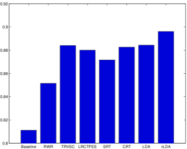
The results of tag reranking are reported in Figure 6. It can be observed that all approaches perform better results than the baseline result. It demonstrates that tag refinement is a useful process. Among these methods, RWR and LDA are based on the tag information and do not take into account of the visual information. SRT only uses the visual information. TRVSC, LRCTPES, CRT and rLDA make use of both the textual and visual information. We can see that both the textual information and the visual information can make great contributions to tag refinement. Though LDA does not use the visual information, it outperforms most of other methods, showing the significant benefit of jointly estimating the tag similarity and the tag relevance and the powerfulness of exploring multi-wise relationships using the topic model. Our approach, rLDA, further improves LDA by encouraging visually similar images having similar topic distributions. The superiority of rLDA over LDA justifies our analysis that rLDA is deeper than LDA illustrated in Figure 2.

The superior performance of our approach can be justified from the deep learning theory [13], which shows that a deeper network has large potentials to achieve better performance. By comparison, the random walk based approaches essentially use shallow structures, which only consists of two levels, the provided tags as the input level and the tag being considered as the output level. The LDA based approach is with a deep structure, introducing a latent topic level, which has potential to get better performance. The proposed regularized LDA model is deeper, with four levels, the tags associated with other images as the first level, the latent topics of other images and the tags of the image being considered as the second level, the latent topic as the third level, and the tag being considered as the output level. The comparison has been illustrated in Figure 2.

5.3.2 Empirical analysis

Figure 6: Performance comparison for tag reranking. The horizontal axis corresponds to different methods, and the vertical axis corresponds to the NDCG score.

Figure 7: Performance comparison of rLDA and LDA with different numbers of topics.

Figure 8: The statistics of the position at which the truly most relevant tag is ranked for our approach. The horizontal axis corresponds to the position and the vertical axis corresponds to the percentage of the images.

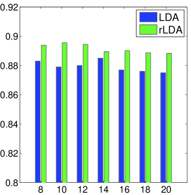
To illustrate the superiority of rLDA over LDA clearer, we compare their performances using different numbers of topics, $K$, which are shown in Figure 7. We have at least two observations. The first one is that taking visual information into account can be effective for the tag refinement task from the fact that rLDA consistently outperforms LDA on different number of topics. The second one is that the performances of both methods begins to decrease when $K$ grows too large. This is reasonable. Considering the extreme case that $K\geqslant V$, it can be validated that it will overfit the data distribution if setting each word as a single topic, which indicates that the relations among tags tend to be useless when $K$ is too large.

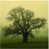
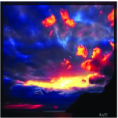
To understand our approach more deeply, we report the percentage of the images in which the truly most relevant tag is ranked in different positions. in Figure 8. We can see that over 60 percent of the images have their most relevant tag at the first position. This can be helpful for related works like image retrieval, group recommendation, etc. Some examples of refined tags are depicted in Figure 9.

Original tags	family winter friends portrait art nature cat nose australia	friends light sunlight paris france water	park winter england cold tree nature	travel summer sun flower nature greece
Refined tags	cat nature portrait nose winter art friends family australia	water light france paris sunlight friends	tree nature winter england park cold	flower nature sun travel summer greece
Original tags	winter sea italy mountain snow alps weather landscape	travel sunset canada tree nature quebec quality	travel sea sky italy landscape sony cielo	england italy cold holland bird grey flight
Refined tags	landscape mountain sea snow winter italy alps weather	sunset tree nature travel quality canada quebec	sky landscape sea travel italy cielo sony	bird flight italy england holland cold grey

Figure 9: Tag ranking examples.

5.4 Results on image retagging

Figure 10: The results of retagging on the NUS-WIDE-LITE dataset. The vertical axis corresponds to F-measure.

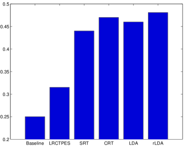
Different from tag reranking, retagging [25] aims to suggest a set of tags that are assigned according to the original tags. These tags may not necessarily be contained in the original tags. In this task, the results of five methods, SRT, LRCTPES, CRT, LDA and our approach, are reported. Other methods based on random walks only produce scores for original tags and can not perform the retagging task Figure 10 shows the experiment results.

The retagging results of all methods outperformed the base line that is based on the original tag list. This demonstrates that image retagging can make significant contributions for image retrieval. In the image retagging task LDA does not perform as good as in the tag reranking task. This is because LDA is unable to deal with the images without tags provided by users, while methods using visual features can tag the images using the tags of similar images. Improving LDA with using visual content of images, our method, rLDA, gets the best result. In both tag reranking and image retagging tasks, the proposed method performs the best, which is because our model is based on a deeper structure and can exploit the semantic information derived from the topic level.

6 Conclusion

This paper presents a regularized latent Dirichlet allocation approach for tag refinement. Our approach succeeds from the factors: (1) Our approach explores the multi-wise relationship among the tags that are mined from both textual and visual information; (2) Our approach explores a deep structure that has large capability to refine tags. Experimental results also demonstrate the superiority of our approach over existing state-of-the-art approaches for tag refinement.

References

- [1] M. Ames and M. Naaman. Why we tag: motivations for annotation in mobile and online media. In CHI, pages 971–980, 2007.
- [2] K. Barnard, P. Duygulu, D. A. Forsyth, N. de Freitas, D. M. Blei, and M. I. Jordan. Matching words and pictures. Journal of Machine Learning Research, 3:1107–1135, 2003.
- [3] Y. Bengio. Learning deep architectures for ai. Foundations and Trends in Machine Learning, 2(1):1–127, 2009.
- [4] D. M. Blei and M. I. Jordan. Modeling annotated data. In SIGIR, pages 127–134, 2003.
- [5] D. M. Blei, A. Y. Ng, and M. I. Jordan. Latent dirichlet allocation. Journal of Machine Learning Research, 3:993–1022, 2003.
- [6] M. Bundschus, S. Yu, V. Tresp, A. Rettinger, and M. Dejori. Hierarchical bayesian models for collaborative tagging systems. In ICDM, 2009.
- [7] G. Carneiro, A. B. Chan, P. J. Moreno, and N. Vasconcelos. Supervised learning of semantic classes for image annotation and retrieval. IEEE Trans. Pattern Anal. Mach. Intell., 29(3):394–410, 2007.
- [8] J. Chang and D. M. Blei. Relational topic models for document networks. Journal of Machine Learning Research - Proceedings Track, 5:81–88, 2009.
- [9] H.-M. Chen, M.-H. Chang, P.-C. Chang, M.-C. Tien, W. H. Hsu, and J.-L. Wu. Sheepdog: group and tag recommendation for flickr photos by automatic search-based learning. In ACM Multimedia, pages 737–740, 2008.
- [10] T.-S. Chua, J. Tang, R. Hong, H. Li, Z. Luo, and Y. Zheng. Nus-wide: a real-world web image database from national university of singapore. In CIVR, 2009.
- [11] R. Datta, D. Joshi, J. Li, and J. Z. Wang. Image retrieval: Ideas, influences, and trends of the new age. ACM Comput. Surv., 40(2), 2008.
- [12] Y. Feng and M. Lapata. Automatic image annotation using auxiliary text information. In ACL, pages 272–280, 2008.
- [13] G. E. Hinton, S. Osindero, and Y. W. Teh. A fast learning algorithm for deep belief nets. Neural Computation, 18(7):1527–1554, 2006.
- [14] J. Jeon and R. Manmatha. Using maximum entropy for automatic image annotation. In CIVR, pages 24–32, 2004.
- [15] W. Jiang, S.-F. Chang, and A. C. Loui. Active context-based concept fusionwith partial user labels. In ICIP, pages 2917–2920, 2006.
- [16] R. Jin, J. Y. Chai, and L. Si. Effective automatic image annotation via a coherent language model and active learning. In ACM Multimedia, pages 892–899, 2004.
- [17] L. S. Kennedy, S.-F. Chang, and I. Kozintsev. To search or to label?: predicting the performance of search-based automatic image classifiers. In Multimedia Information Retrieval, pages 249–258, 2006.
- [18] R. Krestel and P. Fankhauser. Tag recommendation using probabilistic topic models. In ECML/PKDD Discovery Challenge (DC’09), Workshop at ECML/PKDD 2009), 2009.
- [19] R. Krestel, P. Fankhauser, and W. Nejdl. Latent dirichlet allocation for tag recommendation. In RecSys, pages 61–68, 2009.
- [20] J. Li and J. Z. Wang. Automatic linguistic indexing of pictures by a statistical modeling approach. IEEE Trans. Pattern Anal. Mach. Intell., 25(9):1075–1088, 2003.
- [21] X. Li, C. G. M. Snoek, and M. Worring. Learning tag relevance by neighbor voting for social image retrieval. In Multimedia Information Retrieval, pages 180–187, 2008.
- [22] X. Li, C. G. M. Snoek, and M. Worring. Learning social tag relevance by neighbor voting. IEEE Transactions on Multimedia, 11(7):1310–1322, 2009.
- [23] D. Liu, X.-S. Hua, M. Wang, and H.-J. Zhang. Image retagging. In ACM Multimedia, pages 491–500, 2010.
- [24] D. Liu, X.-S. Hua, L. Yang, M. Wang, and H.-J. Zhang. Tag ranking. In WWW, pages 351–360, 2009.
- [25] D. Liu, S. Yan, X.-S. Hua, and H.-J. Zhang. Image retagging using collaborative tag propagation. IEEE Transactions on Multimedia, 13(4):702–712, 2011.
- [26] G. A. Miller. Wordnet: A lexical database for english. Commun. ACM, 38(11):39–41, 1995.
- [27] T. P. Minka. Estimating a dirichlet distribution. Technical report, 2009.
- [28] C.-T. Nguyen, N. Kaothanthong, X. H. Phan, and T. Tokuyama. A feature-word-topic model for image annotation. In CIKM, pages 1481–1484, 2010.
- [29] D. Putthividhya, H. T. Attias, and S. S. Nagarajan. Supervised topic model for automatic image annotation. In ICASSP, pages 1894–1897, 2010.
- [30] G.-J. Qi, X.-S. Hua, Y. Rui, J. Tang, T. Mei, and H.-J. Zhang. Correlative multi-label video annotation. In ACM Multimedia, pages 17–26, 2007.
- [31] B. Sigurbjörnsson and R. van Zwol. Flickr tag recommendation based on collective knowledge. In WWW, pages 327–336, 2008.
- [32] C. Wang, F. Jing, L. Zhang, and H. Zhang. Image annotation refinement using random walk with restarts. In ACM Multimedia, pages 647–650, 2006.
- [33] M. Wang, R. Hong, G. Li, Z.-J. Zha, S. Yan, and T.-S. Chua. Event driven web video summarization by tag localization and key-shot identification. IEEE Transactions on Multimedia, 14(4):975–985, 2012.
- [34] M. Wang, B. Ni, X.-S. Hua, and T.-S. Chua. Assistive tagging: A survey of multimedia tagging with human-computer joint exploration. ACM Comput. Surv., 44(4):25, 2012.
- [35] K. Q. Weinberger, M. Slaney, and R. van Zwol. Resolving tag ambiguity. In ACM Multimedia, pages 111–120, 2008.
- [36] L. Wu, L. Yang, N. Yu, and X.-S. Hua. Learning to tag. In WWW, pages 361–370, 2009.
- [37] H. Xu, J. Wang, X.-S. Hua, and S. Li. Tag refinement by regularized lda. In ACM Multimedia, pages 573–576, 2009.
- [38] N. Zhou, W. K. Cheung, G. Qiu, and X. Xue. A hybrid probabilistic model for unified collaborative and content-based image tagging. IEEE Trans. Pattern Anal. Mach. Intell., 33(7):1281–1294, 2011.
- [39] G. Zhu, S. Yan, and Y. Ma. Image tag refinement towards low-rank, content-tag prior and error sparsity. In ACM Multimedia, pages 461–470, 2010.