Optimal Rate Sampling in 802.11 Systems

Richard Combes, Alexandre Proutiere†,×, Donggyu Yun, Jungseul Ok, Yung Yi {\dagger}: KTH Royal Institute of Technology, Sweden. ×\times: INRIA/Microsoft joint research centre, Palaiseau, France. {\ddagger}: Department of Electrical Engineering, KAIST, South Korea.
Abstract

Rate Adaptation (RA) is a fundamental mechanism in 802.11 systems. It allows transmitters to adapt the coding and modulation scheme as well as the MIMO transmission mode to the radio channel conditions, and in turn, to learn and track the (mode, rate) pair providing the highest throughput. So far, the design of RA mechanisms has been mainly driven by heuristics. In contrast, in this paper, we rigorously formulate such design as an online stochastic optimisation problem. We solve this problem and present ORS (Optimal Rate Sampling), a family of (mode, rate) pair adaptation algorithms that provably learn as fast as it is possible the best pair for transmission. We study the performance of ORS algorithms in both stationary radio environments where the successful packet transmission probabilities at the various (mode, rate) pairs do not vary over time, and in non-stationary environments where these probabilities evolve. We show that under ORS algorithms, the throughput loss due to the need to explore sub-optimal (mode, rate) pairs does not depend on the number of available pairs, which is a crucial advantage as evolving 802.11 standards offer an increasingly large number of (mode, rate) pairs. We illustrate the efficiency of ORS algorithms (compared to the state-of-the-art algorithms) using simulations and traces extracted from 802.11 test-beds.

1 Introduction

In wireless communication systems, Rate Adaptation (RA) is a fundamental mechanism allowing transmitters to adapt the coding and modulation scheme to the radio channel conditions. In 802.11 systems, the transmitter may choose from a finite set of rates with the objective of identifying as fast as possible the rate providing maximum throughput, i.e., maximising the product of the rate and the successful packet transmission probability. The challenge stems from the facts that these probabilities are not known a priori at the transmitter, and that they may evolve over time. The transmitter has to learn and track the best transmission rate, based on the measurements and observations made on the successive packet transmissions.

Over the last decade, a large array of RA mechanisms for 802.11 systems has been proposed. We may categorise these mechanisms depending on the feedback and measurements from past transmissions available at the transmitter, and actually used to sequentially select rates for packet transmissions. Traditionally in 802.11 systems, RA mechanisms are based on rate sampling approaches, i.e., the rate selection solely depends on the number of successes and failures of previous packet transmissions at the various available rates. Examples of such mechanisms include ARF (Auto Rate Fall back) [19] and SampleRate [4]. As 802.11 standards evolve, the number of available rates increases. In 802.11n systems, for a given packet transmission, a MIMO mode (e.g. a diversity oriented single-stream (SS) mode or a spatial multiplexing driven double-stream (DS) mode) and a rate have to be jointly selected. The number of possible decisions can then become quite large, making the use of sampling approaches questionable.

A natural alternative to RA sampling approaches consists in using channel measurements. So far, such measurements have not been explicitly used in practice. The most accessible measurement, the receiver signal strength indication (RSSI), is known to lead to poor predictions of the packet error rate (PER) at the various rates (see e.g. [2, 29, 6, 39, 14, 8]). These poor predictions are for example due to the fact that RSSI does not reflect frequency-selective fading. Note that 802.11n NICs actually measure and report the channel quality at the OFDM subcarrier level, also known as channel state information (CSI), which provides better information than the simple RSSI. CSI feedback could be used to improve PER prediction accuracy [14]. However it is difficult and costly to get and store this complete information [7], and CSI feedback is supported by very few 802.11n devices. A promising solution could then consist in storing and using only parts of this information, as proposed for example in [8].

As of now, it seems difficult to predict whether measurement-based RA mechanisms will be widely adopted in the future, or whether rate sampling approaches will continue to prevail. In this paper, we investigate the fundamental performance limits of sampling-based RA mechanisms. Our objective is to design the best possible rate sampling algorithm, i.e., the algorithm that identifies as fast as possible the rate maximising throughput. Our approach departs from previous methods to design RA mechanisms: in existing mechanisms, the way sub-optimal rates are explored to learn and track the best rate for transmission is based on heuristics. In contrast, we look for the optimal way of exploring sub-optimal rates.

We rigorously formulate the design of the best rate sampling algorithm as an online stochastic optimisation problem. In this problem, the objective is to maximise the number of packets successfully sent over a finite time horizon. We show that this problem reduces to a Multi-Armed Bandit (MAB) problem [24]. In MAB problems, a decision maker sequentially selects an action (or an arm), and observes the corresponding reward. Rewards of a given arm are random variables with unknow distribution. The objective is to design sequential action selection strategies that maximise the expected reward over a given time horizon. These strategies have to achieve an optimal trade-off between exploitation (actions that has provided high rewards so far have to be selected) and exploration (sub-optimal actions have to be chosen so as to learn their average rewards). For the rate adaptation problem, the various arms correspond to the decisions available at the transmitter to send packets, i.e., in 802.11a/b/g systems, an arm corresponds to a modulation and coding scheme or equivalently to a transmission rate, whereas in MIMO 802.11n systems, an arm corresponds to a (mode, rate) pair. When a rate is selected for a packet transmission, the reward is equal to 1 if the transmission is successful, and equal to 0 otherwise. The average successful packet transmission probabilities at the various rates are of course unknown, and have to be learnt.

The sequential rate (or (mode, rate) in MIMO 802.11n systems) selection problem is referred to as a structured MAB problem in the following, as it differs from classical MAB problems. First, the rewards associated with the various rates are stochastically correlated, i.e., the outcomes of transmissions at different rates are not independent: for example, if a transmission at a high rate is successful, it would be also successful at lower rates. Then, the average throughputs achieved at various rates exhibit natural structural properties. For 802.11b/g systems, the throughput is an unimodal function of the selected rate. For MIMO 802.11n systems, the throughput remains unimodal in the rates within a single MIMO mode, and also satisfies some structural properties across modes. We model the throughput as a so-called graphically unimodal function of the (mode, rate) pair. As we demonstrate, correlations and graphical unimodality are instrumental in the design of RA mechanisms, and can be exploited to learn and track the best rate or (mode, rate) pair quickly and efficiently. Finally, most MAB problems consider stationary environments, which, for our problem, means that the successful packet transmission probabilities at different rates do not vary over time. In practice, the transmitter faces a non-stationary environment as these probabilities could evolve over time. We consider both stationary and non-stationary radio environements.

In the case of stationary environments, we derive an asymptotic upper bound of the expected reward achieved in structured MAB problems. This provides a fundamental performance limit satisfied by any rate adaptation algorithm. This limit quantifies the inevitable performance loss due to the need to explore sub-optimal rates. It also indicates the performance gains that can be achieved by devising rate adaptation schemes that optimally exploit the correlations and the structural properties of the MAB problem. As it turns out, the performance loss due to the need of exploration does not depend on the number of available rates (or (mode, rate) pairs), i.e., on the size of the decision space. This suggests that rate sampling methods can perform well even if the number of decisions available at the transmitter grows large. We present two rate sampling algorithms: ORS (Optimal Rate Sampling) and G-ORS (G stands for Graphical), an extension of ORS to MIMO systems. We show that their performance matches the upper bound derived previously, i.e., ORS and G-ORS are asymptotically optimal. We extend the results and algorithms to non-stationary radio environments: we propose SW-ORS and SW-G-ORS algorithms (SW stands for Sliding Window) and analyse their performance. We show that again, the latter does not depend on the size of the decision space, and that the best rate (or (mode, rate) pair) can be efficiently learnt and tracked even. Finally we compare the performance of the proposed algorithms to that of existing rate sampling algorithms using simulations and traces extracted from real 802.11 test-beds. Our algorithms outperform existing RA schemes. This should not be surprising: the design of most existing algorithms is based on heuristics, whereas ORS algorithms are by design optimal.

Contributions and paper organisation.

  1. 1.

    The next section is devoted to the related work. Existing RA algorithms (using either sampling approaches, or based on measurements) are discussed. A brief state-of-the-art about MAB problems is also presented.

  2. 2.

    In the next two sections (Sections 3 and 4), we formulate the design of rate sampling algorithms as an online stochastic optimization problem, and we show how the latter can be mapped to a structured MAB problem.

  3. 3.

    We derive a performance upper bound satisfied by any rate sampling algorithm in the case of stationary radio environements, and show that this bound does not depend on the size of the decision space (Section 5).

  4. 4.

    We present, in Section 6, ORS, a rate sampling algorithm whose performance matches the upper bound derived in Section 5.

  5. 5.

    Next in Section 7, we present SW-ORS, an extension of ORS to non-stationary radio environments and provide guarantees on its performance. Again we show that its performance does not depend on the number of available rates.

  6. 6.

    The algorithms and performance results are extended to MIMO 802.11n systems in Section 8. The proposed algorithm, referred to as G-ORS (G stands for Graphical), optimally exploits the fact that the throughput is a graphically unimodal function of the (mode, rate) pair.

  7. 7.

    Finally in Section 9, the performance of our algorithms are illustrated using simulation results and traces extratced from real 802.11 test-beds.

2 Related work

2.1 RA mechanisms in 802.11 systems

In recent years, there has been a growing interest in the design of RA mechanisms for 802.11 systems, perhaps motivated by the new functionalities (e.g. MIMO, and channel width adaptation) offered by the evolving standards.

Sampling-based RA mechanisms. ARF [19], one of the earliest rate adaptation algorithms, consists in changing the transmission rate based on packet loss history: a higher rate is probed after n𝑛n consecutive successful packet transmissions, and the next available lower rate is used after two consecutive packet losses. In case of stationary radio environments, ARF essentially probe higher rates too frequently (every 10 packets or so). To address this issue, AARF [23] adapts the threshold n𝑛n dynamically to the speed at which the radio environment evolves. Among other proposals, SampleRate [4] sequentially selects transmission rates based on estimated throughputs over a sliding window, and has been shown to outperform ARF and its variants. The aforementioned algorithms were initially designed for 802.11 a/b/g systems, and they seem to perform poorly in MIMO 802.11n systems [27]. One of the reasons for this poor performance is the non-monotonic relation between loss and rate in 802.11n MIMO systems, when considering all rates options and ignoring modes. When modes are ignored, the loss probability does not necessarily increase with the rate. As a consequence, RA mechanisms that ignore modes may get stuck at low rates. To overcome this issue, the authors of [27] propose MiRA, a RA scheme that zigzags between MIMO modes to search for the best (mode, rate) pair. In the design of RAMAS [25], the authors categorise the different types of modulations into modulation-groups, as well as the MIMO modes into what is referred to as enhancement groups; the combination of the modulation and enhancement group is mapped back to the set of the modulation and coding schemes. RAMAS then adapts these two groups concurrently. As a final remark, note that in 802.11 systems, packet losses are either due to a mismatch between the rate selection and the channel condition or due to collisions with transmissions of other transmitters. Algorithms such as LD-ARF [26], CARA [21], and RRAA [36] have been proposed to distinguish between losses and collisions.

It is important to highlight the fact that in all the aforementioned RA algorithms, the way sub-optimal rates (or (mode, rate) pairs) are explored to identify the best rate is based on heuristics. This contrasts with the proposed algorithms, that are designed, using stochastic optimisation methods, to learn the best rate for transmission as fast as possible. The way sub-optimal rates are explored under our algorithms is optimal.

Measurement-based methods. As mentioned in the introduction, measurement-based RA algorithms could outperform sampling approaches if the measurements (RSSI or CSI) used at the transmitter could be used to accurately predict the PER achieved at the various rates. However this is not always the case, and measurement-based approaches incur an additional overhead by requiring the receiver to send channel-state information back to the transmitter. In fact, sampling and measurement-based approaches have their own advantages and disadvantages. We report here a few measurement-based RA mechanisms.

In RBAR [17] (developed for 802.11 a/b/g systems), RTS/CTS-like control packets are used to “probe” the channel. The receiver first computes the best rate based on the SNR measured over an RTS packet and then informs the transmitter about this rate using the next CTS packet. OAR [31] is similar to RBAR, but lets the transmitter send multiple back-to-back packets without repeating contention resolution procedure. CHARM [18] leverages the channel reciprocity to estimate the SNR value instead of exchanging RTS/CTS packets. In 802.11n with MIMO, ARAMIS [8] uses the so-called diffSNR as well as the SNR to predict the PER at each rate. The diffSNR corresponds to the difference between the maximum and minimum SNRs observed on the various antennas at the receiver. ARAMIS exploits the fact that environmental factors (e.g., scattering, positioning) are reflected in the diffSNR. Recently, hybrid approaches combining SNR measurements and sampling techniques have also been advocated, see [15]. It is also worth mentioning cross-layer approaches, as in [35], where BER (Bit Error Rate) are estimated using information provided at the physical layer.

In some sense, measurement-based RA schemes in 802.11 systems try to mimic rate adaptation strategies used in cellular networks. However in these networks, more accurate information on channel condition is provided to base station [1]. Typically, the base station broadcasts a pilot signal, from which each receiver measures the channel conditions. The receiver sends this measurement, referred to as CQI (Channel Quality Indicator), back to the base station. The transmission rate is then determined by selecting the highest CQI value which satisfies the given BLER (Block Error Rate) threshold, e.g., 10% in 3G systems. More complex, but also more efficient rate selection mechanisms are proposed in [20, 9]. These schemes predict the throughput more accurately by jointly considering other mechanisms used at the physical layer, such as HARQ (Hybrid ARQ).

2.2 Stochastic MAB problems

Stochastic MAB formalise sequential decision problems where the decision maker has to strike an optimal trade-off between exploitation and exploration. MAB problems have been applied in many disciplines – their first application was in the context of clinical trials [34]. Please refer to [5] for a recent survey. Most existing theoretical results concern unstructured MAB problems [30], i.e., problems where the average reward associated with the various arms are not related. For this kind of problems, Lai and Robbins [24] derived an asymptotic lower bound on regret and also designed optimal decision algorithms. When the average rewards are structured, the design of optimal decision algorithms is more challenging, see e.g. [5]. Unimodal bandit problems have received little attention so far. In [38], the authors propose various algorithms, but they do not prove their optimality (the . In this paper, we first derive asymptotic regret lower bounds for these problems, and then devise asymptotically optimal algorithms. We also study unimodal bandit problems in non-stationary environments, where the average rewards of the different arms evolve over time. Non-stationary environments have not been extensively studied in the bandit literature. For unstructured problems, the performance of algorithms based on UCB [3] has been analyzed in [22, 37, 12] under the assumption that the average rewards are abruptely changing. Here we consider more realistic scenarios where the average rewards smoothly evolve over time. To our knowledge, such scenarios have only been considered in [33, 32] but using different assumptions. Finally, the authors of [28] formalize rate adaptation and channel selection issues as a MAB problem, but they do not solve it, and the proposed algorithms are heuristics.

3 Models and Objectives

We present here the models and objectives for 802.11 a/b/g systems (using a single MIMO mode). The extension to MIMO 802.11n is discussed in Section 8. We consider a single link (a transmitter-receiver pair). At time 0, the link becomes active and the transmitter has packets to send to the receiver. To do so, the transmitter can sequentially pick a coding rate from a finite set ={r1,,rK}subscript𝑟1subscript𝑟𝐾{\cal R}=\{r_{1},\ldots,r_{K}\}. This set is ordered, i.e., r1<r2<<rKsubscript𝑟1subscript𝑟2subscript𝑟𝐾r_{1}<r_{2}<\ldots<r_{K}. After a packet is sent, the transmitter is informed on whether the transmission has been successful. Based on the observed past transmission successes and failures at the various rates, the transmitter has to select a rate for the next packet transminssion. We denote by ΠΠ\Pi the set of all possible sequential rate selection schemes. Packets are assumed to be of equal size, and without loss of generality the duration of a packet transmission at rate rksubscript𝑟𝑘r_{k} is 1/rk1subscript𝑟𝑘1/r_{k} for any k𝑘k.

3.1 Channel models

For the i𝑖i-th packet transmission at rate rksubscript𝑟𝑘r_{k}, a binary random variable Xk(i)subscript𝑋𝑘𝑖X_{k}(i) represents the success (Xk(i)=1subscript𝑋𝑘𝑖1X_{k}(i)=1) or failure (Xk(i)=0subscript𝑋𝑘𝑖0X_{k}(i)=0) of the transmission.

Stationary radio environments. In such environments, the success transmission probabilities at different rates do not evolve over time. This arises when the system considered is static (in particular, the transmitter and receiver do not move) – refer to Section VI for a detailed discussion. Formally, Xk(i)subscript𝑋𝑘𝑖X_{k}(i), i=1,2,𝑖12i=1,2,\ldots, are independent and identically distributed, and we denote by θksubscript𝜃𝑘\theta_{k} the success transmission probability at rate rksubscript𝑟𝑘r_{k}: θk=𝔼[Xk(i)]subscript𝜃𝑘𝔼delimited-[]subscript𝑋𝑘𝑖\theta_{k}=\mathbb{E}[X_{k}(i)]. We denote by ksuperscript𝑘k^{\star} the index of the optimal rate, kargmaxkrkθksuperscript𝑘subscript𝑘subscript𝑟𝑘subscript𝜃𝑘k^{\star}\in\arg\max_{k}r_{k}\theta_{k}. To simplify the exposition and the notation, we assume that the optimal rate is unique, i.e., rkθk>rkθksubscript𝑟superscript𝑘subscript𝜃superscript𝑘subscript𝑟𝑘subscript𝜃𝑘r_{k^{\star}}\theta_{k^{\star}}>r_{k}\theta_{k}, for all kk𝑘superscript𝑘k\neq k^{\star}.

Non-stationary radio environments. In practice, channel conditions may be non-stationary, i.e., the success probabilities at various rates could evolve over time. In many situations, the evolution over time is rather slow – refer to [28] and to Section V for test-bed measurements. These slow variations allow us to devise rate adaptation schemes that efficiently track the best rate for transmission. In the case of non-stationary environment, we denote by θk(t)subscript𝜃𝑘𝑡\theta_{k}(t) the success transmission probability at rate rksubscript𝑟𝑘r_{k} and at time t𝑡t, and by k(t)superscript𝑘𝑡k^{\star}(t) the index of the optimal rate at time t𝑡t.

Unless otherwise specified, for clarity, we consider stationary radio environments. Non-stationary environements are treated in Section 7, where we will present the models and objectives, and extend our rate selection algorithm for these scenarios.

3.2 Structural properties

Our problem is to identify as fast as possible the rate maximizing throughput. To this aim, we shall desin algorithms that exploit two crucial structural properties of the problem: (i) The successes and failures of transmissions at various rates are correlated, and (ii) in practice, we have observed that the throughput is an unimodal function of the transmission rate.

Correlations. If a transmission is successful at a high rate, it has to be successful at a lower rate, and similarly, if a low-rate transmission fails, then a transmitting at a higher rate would also fail. Formally assume that at a given time, rate rksubscript𝑟𝑘r_{k} (resp. rate rlsubscript𝑟𝑙r_{l}) has already been selected (i1)𝑖1(i-1) (resp. (j1)𝑗1(j-1)) times. Then:

(k<l and Xk(i)=0)(Xl(j)=0),𝑘𝑙 and subscript𝑋𝑘𝑖0subscript𝑋𝑙𝑗0\left(k<l\hbox{ and }X_{k}(i)=0\right)\Longrightarrow(X_{l}(j)=0), (1)
(k>l and Xk(i)=1)(Xl(j)=1).𝑘𝑙 and subscript𝑋𝑘𝑖1subscript𝑋𝑙𝑗1\left(k>l\hbox{ and }X_{k}(i)=1\right)\Longrightarrow(X_{l}(j)=1). (2)

Using simple coupling arguments, we can readily show that an equivalent way of expressing the correlations is to state that the following assumption holds.

Assumption 1

θ=(θ1,,θK)𝒯𝜃subscript𝜃1subscript𝜃𝐾𝒯\theta=(\theta_{1},\ldots,\theta_{K})\in{\cal T}, where 𝒯={η[0,1]K:η1ηK}𝒯conditional-set𝜂superscript01𝐾subscript𝜂1subscript𝜂𝐾{\cal T}=\{\eta\in[0,1]^{K}:\eta_{1}\geq\ldots\geq\eta_{K}\}.

Unimodality. In practice, we observe that the throughputs achieved by transmitting at various rates are unimodal. To formalize this observation, we make the following assumption, that will be extensively discussed and verified in Section 9.

Assumption 2

θ𝒰𝜃𝒰\theta\in{\cal U}, where 𝒰={η[0,1]K:k,r1η1<<rkηk,rkηk>rk+1ηk+1>>rkηK}𝒰conditional-set𝜂superscript01𝐾formulae-sequencesuperscript𝑘subscript𝑟1subscript𝜂1subscript𝑟superscript𝑘subscript𝜂superscript𝑘subscript𝑟superscript𝑘subscript𝜂superscript𝑘subscript𝑟superscript𝑘1subscript𝜂superscript𝑘1subscript𝑟𝑘subscript𝜂𝐾{\cal U}=\{\eta\in[0,1]^{K}:\exists k^{\star},r_{1}\eta_{1}<\ldots<r_{k^{\star}}\eta_{k^{\star}},r_{k^{\star}}\eta_{k^{\star}}>r_{k^{\star}+1}\eta_{k^{\star}+1}>\ldots>r_{k}\eta_{K}\}.

3.3 Objective

We now formulate the design of rate adaptation schemes as an online stochastic optimization problem. An optimal scheme maximizes the expected throughput up to a certain finite time T𝑇T. The choice of T𝑇T is not really important as long as during time interval T𝑇T, a large number of packets can be sent – so that infering the success transmission probabilities efficiently is possible.

Consider a rate adaption scheme πΠ𝜋Π\pi\in\Pi that selects rate rkπ(t)subscript𝑟superscript𝑘𝜋𝑡r_{k^{\pi}(t)} for the t𝑡t-th transmission. At time T𝑇T, the number of packets γπ(T)superscript𝛾𝜋𝑇\gamma^{\pi}(T) that have been successfully sent under algorithm π𝜋\pi is: γπ(T)=ki=1skπ(T)Xk(i)superscript𝛾𝜋𝑇subscript𝑘superscriptsubscript𝑖1superscriptsubscript𝑠𝑘𝜋𝑇subscript𝑋𝑘𝑖\gamma^{\pi}(T)=\sum_{k}\sum_{i=1}^{s_{k}^{\pi}(T)}X_{k}(i), where skπ(T)superscriptsubscript𝑠𝑘𝜋𝑇s_{k}^{\pi}(T) is the number of transmission attempts at rate rksubscript𝑟𝑘r_{k} before time T𝑇T. The sk(T)subscript𝑠𝑘𝑇s_{k}(T)’s are random variables (since the rates selected under π𝜋\pi depend on the past random successes and failures), and satisfy the following constraint:

kskπ(T)×1rkT.subscript𝑘superscriptsubscript𝑠𝑘𝜋𝑇1subscript𝑟𝑘𝑇\sum_{k}s_{k}^{\pi}(T)\times{1\over r_{k}}\leq T.

Wald’s lemma implies that the expected number of packets successfully sent up to time T𝑇T is: 𝔼[γπ(T)]=k𝔼[skπ(T)]θk.𝔼delimited-[]superscript𝛾𝜋𝑇subscript𝑘𝔼delimited-[]superscriptsubscript𝑠𝑘𝜋𝑇subscript𝜃𝑘\mathbb{E}[\gamma^{\pi}(T)]=\sum_{k}\mathbb{E}[s_{k}^{\pi}(T)]\theta_{k}. Thus, our objective is to design an algorithm solving the following online stochastic optimization problem:

maxπΠsubscript𝜋Π\displaystyle\max_{\pi\in\Pi} k𝔼[skπ(T)]θk,subscript𝑘𝔼delimited-[]superscriptsubscript𝑠𝑘𝜋𝑇subscript𝜃𝑘\displaystyle\sum_{k}\mathbb{E}[s_{k}^{\pi}(T)]\theta_{k}, (3)
s.t. skπ(T), and kskπ(T)×1rkT,k.formulae-sequencesuperscriptsubscript𝑠𝑘𝜋𝑇 and subscript𝑘superscriptsubscript𝑠𝑘𝜋𝑇1subscript𝑟𝑘𝑇for-all𝑘\displaystyle s_{k}^{\pi}(T)\in\mathbb{N},\hbox{ and }\sum_{k}s_{k}^{\pi}(T)\times{1\over r_{k}}\leq T,\quad\forall k.

4 An equivalent Structured Multi-Armed Bandit (MAB) problem

In this section, we show that the online optimization problem (3) can be reduced to a structured Multi-Armed Bandit (MAB) problem.

4.1 An alternative system

Without loss of generality, we assume that time can be divided into slots whose durations are such that for any k𝑘k, the time it takes to transmit one packet at rate rksubscript𝑟𝑘r_{k} corresponds to an integer number of slots. Under this convention, the optimization problem (3) can be written as:

maxπΠsubscript𝜋Π\displaystyle\max_{\pi\in\Pi} k𝔼[tkπ(T)]rkθk,subscript𝑘𝔼delimited-[]superscriptsubscript𝑡𝑘𝜋𝑇subscript𝑟𝑘subscript𝜃𝑘\displaystyle\sum_{k}\mathbb{E}[t_{k}^{\pi}(T)]r_{k}\theta_{k}, (4)
s.t. ktkπ(T)T, andsubscript𝑘superscriptsubscript𝑡𝑘𝜋𝑇𝑇 and\displaystyle\sum_{k}t_{k}^{\pi}(T)\leq T,\hbox{ and }
tkπ(T)1rk:={urk,u},k,formulae-sequencesuperscriptsubscript𝑡𝑘𝜋𝑇1subscript𝑟𝑘assign𝑢subscript𝑟𝑘𝑢for-all𝑘\displaystyle t_{k}^{\pi}(T)\in{1\over r_{k}}\mathbb{N}:=\{{u\over r_{k}},u\in\mathbb{N}\},\forall k,

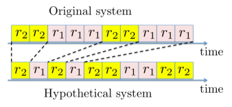
where tkπ(T)=skπ(T)/rksuperscriptsubscript𝑡𝑘𝜋𝑇superscriptsubscript𝑠𝑘𝜋𝑇subscript𝑟𝑘t_{k}^{\pi}(T)=s_{k}^{\pi}(T)/r_{k} represents the amount of time (in slots) that the transmitter spends, before T𝑇T, on sending packets at rate rksubscript𝑟𝑘r_{k}. The constraint tk(T)1rksubscript𝑡𝑘𝑇1subscript𝑟𝑘t_{k}(T)\in{1\over r_{k}}\mathbb{N} indicates that when a rate is selected, this rate selection remains the same for the next 1/rk1subscript𝑟𝑘1/r_{k} slots (to transmit an entire packet). By relaxing this constraint, we obtain an optimization problem corresponding to a MAB problem. Indeed, consider now an alternative system where rate selection is made every slot. If at any given slot, rate rksubscript𝑟𝑘r_{k} is selected for the i𝑖i-th times, then if Xk(i)=1subscript𝑋𝑘𝑖1X_{k}(i)=1, the transmitter successfully sends rksubscript𝑟𝑘r_{k} bits in this slot, and if Xk(i)=0subscript𝑋𝑘𝑖0X_{k}(i)=0, then no bit are received. A rate selection algorithm then decides in each slot which rate to use. There is a natural mapping between rate selection algorithms in the original system and in the alternative system: let πΠ𝜋Π\pi\in\Pi, if for the t𝑡t-th packet transmission rate rksubscript𝑟𝑘r_{k} is selected under π𝜋\pi in the original system, then π𝜋\pi selects the same rate rksubscript𝑟𝑘r_{k} in the t𝑡t-th slot. This mapping is illustrated in Figure 1.
Refer to caption
Figure 1: Examples of rate selections made by the same algorithm πΠ𝜋Π\pi\in\Pi in the original and alternative systems - r1=1/3subscript𝑟113r_{1}=1/3 and r2=1/2subscript𝑟212r_{2}=1/2.

For the alternative system, the objective is to design πΠ𝜋Π\pi\in\Pi solving the following optimization problem, which can be interpreted as a relaxation of (4).

maxπΠsubscript𝜋Π\displaystyle\max_{\pi\in\Pi} k𝔼[tkπ(T)]rkθk,subscript𝑘𝔼delimited-[]superscriptsubscript𝑡𝑘𝜋𝑇subscript𝑟𝑘subscript𝜃𝑘\displaystyle\sum_{k}\mathbb{E}[t_{k}^{\pi}(T)]r_{k}\theta_{k}, (5)
s.t. ktkπ(T)T, and tkπ(T),k.formulae-sequencesubscript𝑘superscriptsubscript𝑡𝑘𝜋𝑇𝑇 and superscriptsubscript𝑡𝑘𝜋𝑇for-all𝑘\displaystyle\sum_{k}t_{k}^{\pi}(T)\leq T,\hbox{ and }t_{k}^{\pi}(T)\in\mathbb{N},\forall k.

The above optimization problem corresponds to a MAB problem, where in each slot a decision is taken (i.e., a rate is selected), and where when rate rksubscript𝑟𝑘r_{k} is chosen, the obtained reward is rksubscript𝑟𝑘r_{k} with probability θksubscript𝜃𝑘\theta_{k} and 0 with probability 1θk1subscript𝜃𝑘1-\theta_{k}. Note that in traditional MAB problems, the rewards obtained by taking various decisions are stochastically independent. This is not the case for our MAB problem.

4.2 Regrets and Asymptotic Equivalence

We may assess the performance of an algorithm πΠ𝜋Π\pi\in\Pi in both original and alternative systems through the notion of regret. The regret up to slot T𝑇T compares the performance of π𝜋\pi to that achieved by an algorithm always selecting the best rate. If the parameter θ𝜃\theta was known, then in both systems, it would be optimal to select rate rksubscript𝑟superscript𝑘r_{k^{\star}}. The regret of algorithm π𝜋\pi up to time slot T𝑇T in the original system is then defined by:

R1π(T)=θkrkTkθk𝔼[skπ(T)],superscriptsubscript𝑅1𝜋𝑇subscript𝜃superscript𝑘subscript𝑟superscript𝑘𝑇subscript𝑘subscript𝜃𝑘𝔼delimited-[]superscriptsubscript𝑠𝑘𝜋𝑇R_{1}^{\pi}(T)=\theta_{k^{\star}}\lfloor r_{k^{\star}}T\rfloor-\sum_{k}\theta_{k}\mathbb{E}[s_{k}^{\pi}(T)],

where x𝑥\lfloor x\rfloor denotes the largest integer smaller than x𝑥x.

The regret of algorithm π𝜋\pi up to time slot T𝑇T in the alternative system is similarly defined by:

Rπ(T)=θkrkTkθkrk𝔼[tkπ(T)].superscript𝑅𝜋𝑇subscript𝜃superscript𝑘subscript𝑟superscript𝑘𝑇subscript𝑘subscript𝜃𝑘subscript𝑟𝑘𝔼delimited-[]superscriptsubscript𝑡𝑘𝜋𝑇R^{\pi}(T)=\theta_{k^{\star}}r_{k^{\star}}T-\sum_{k}\theta_{k}r_{k}\mathbb{E}[t_{k}^{\pi}(T)].

In the next section, we show that an asymptotic lower bound for the regret Rπ(T)superscript𝑅𝜋𝑇R^{\pi}(T) is of the form c(θ)log(T)𝑐𝜃𝑇c(\theta)\log(T) where c(θ)𝑐𝜃c(\theta) is a strictly positive constant that we can explicitly characterize. It means that for all πΠ𝜋Π\pi\in\Pi, liminfTRπ(T)/log(T)c(θ)subscriptinfimum𝑇superscript𝑅𝜋𝑇𝑇𝑐𝜃\lim\inf_{T\to\infty}R^{\pi}(T)/\log(T)\geq c(\theta). It will be also shown that there exists an algorithm πΠsuperscript𝜋Π\pi^{\star}\in\Pi that actually achieves this lower bound in the alternative system, in the sense that limsupTRπ(T)/log(T)c(θ)subscriptsupremum𝑇superscript𝑅superscript𝜋𝑇𝑇𝑐𝜃\lim\sup_{T\to\infty}R^{\pi^{\star}}(T)/\log(T)\leq c(\theta). In such a case, we say that πsuperscript𝜋\pi^{\star} is asymptotically optimal. The following lemma states that actually, the same lower bound is valid in the original system, and that any asymptotically optimal algorithm in the alternative system is also asymptotically optimal in the original system.

Lemma 4.1

Let πΠ𝜋Π\pi\in\Pi. For any c>0𝑐0c>0, we have:

(liminfTRπ(T)log(T)c)(liminfTR1π(T)log(T)c),subscriptinfimum𝑇superscript𝑅𝜋𝑇𝑇𝑐subscriptinfimum𝑇superscriptsubscript𝑅1𝜋𝑇𝑇𝑐\left(\lim\inf_{T\to\infty}{R^{\pi}(T)\over\log(T)}\geq c\right)\Longrightarrow\left(\lim\inf_{T\to\infty}{R_{1}^{\pi}(T)\over\log(T)}\geq c\right),

and

(limsupTRπ(T)log(T)c)(limsupTR1π(T)log(T)c).subscriptsupremum𝑇superscript𝑅𝜋𝑇𝑇𝑐subscriptsupremum𝑇superscriptsubscript𝑅1𝜋𝑇𝑇𝑐\left(\lim\sup_{T\to\infty}{R^{\pi}(T)\over\log(T)}\leq c\right)\Longrightarrow\left(\lim\sup_{T\to\infty}{R_{1}^{\pi}(T)\over\log(T)}\leq c\right).

Proof. Let T>0𝑇0T>0. By time T𝑇T, we know that there have been at least Tr1𝑇subscript𝑟1\lfloor Tr_{1}\rfloor transmissions, but no more than TrK𝑇subscript𝑟𝐾\lceil Tr_{K}\rceil. Also observe that both regrets Rπsuperscript𝑅𝜋R^{\pi} and R1πsubscriptsuperscript𝑅𝜋1R^{\pi}_{1} are increasing functions of time. We deduce that:

Rπ(Tr1)R1π(T)Rπ(TrK).superscript𝑅𝜋𝑇subscript𝑟1superscriptsubscript𝑅1𝜋𝑇superscript𝑅𝜋𝑇subscript𝑟𝐾R^{\pi}(\lfloor Tr_{1}\rfloor)\leq R_{1}^{\pi}(T)\leq R^{\pi}(\lceil Tr_{K}\rceil).

Now

liminfTR1π(T)log(T)subscriptinfimum𝑇superscriptsubscript𝑅1𝜋𝑇𝑇\displaystyle\lim\inf_{T\to\infty}{R_{1}^{\pi}(T)\over\log(T)} liminfTRπ(Tr1)log(T)absentsubscriptinfimum𝑇superscript𝑅𝜋𝑇subscript𝑟1𝑇\displaystyle\geq\lim\inf_{T\to\infty}{R^{\pi}(\lfloor Tr_{1}\rfloor)\over\log(T)}
=liminfTRπ(Tr1)log(Tr1)c.absentsubscriptinfimum𝑇superscript𝑅𝜋𝑇subscript𝑟1𝑇subscript𝑟1𝑐\displaystyle=\lim\inf_{T\to\infty}{R^{\pi}(\lfloor Tr_{1}\rfloor)\over\log(\lfloor Tr_{1}\rfloor)}\geq c.

The second statement can be derived similarly. \Box

4.3 Structured MAB problem

Instead of trying to solve (3), we rather focus on analyzing the MAB problem (5). We know that optimal algorithms for (5) will also be optimal for the original problem. As already mentioned, the specificity of our MAB problem lies in its structure, i.e., in the correlations and unimodality of the rewards obtained using different rates. Let us summarize the problem:

(PU)subscript𝑃𝑈(P_{U}) structured MAB. We have a set {1,,K}1𝐾\{1,\ldots,K\} of possible decisions. If decision k𝑘k is taken for the i𝑖i-th time, we received a reward rkXk(i)subscript𝑟𝑘subscript𝑋𝑘𝑖r_{k}X_{k}(i). (Xk(i),i=1,2,)formulae-sequencesubscript𝑋𝑘𝑖𝑖12(X_{k}(i),i=1,2,...) are i.i.d. with Bernoulli distribution with mean θksubscript𝜃𝑘\theta_{k}. The structure of rewards across decisions are expressed through Assumptions 1 and 2, or equivalently θ𝒯𝒰𝜃𝒯𝒰\theta\in{\cal T}\cap{\cal U}. The objective is to design a decision scheme minimizing the regret Rπ(T)superscript𝑅𝜋𝑇R^{\pi}(T) over all possible algorithms πΠ𝜋Π\pi\in\Pi.

5 Lower bound on regret

In this section, we derive an asymptotic (as T𝑇T grows large) lower bound of the regret Rπ(T)superscript𝑅𝜋𝑇R^{\pi}(T) satisfied by any algorithm πΠ𝜋Π\pi\in\Pi. This lower bound provides an insightful theoretical performance limit for any rate adaptation scheme. We also quantify the performance gains achieved by algorithms that smartly exploit the structural properties of (PUsubscript𝑃𝑈P_{U}), compared to algorithms that consider the rewards obtained at various rates as independent.

5.1 Structured MAB

To derive a lower bound on regret for MAB problem (PUsubscript𝑃𝑈P_{U}), we first introduce the notion of uniformly good algorithms. An algorithm π𝜋\pi is uniformly good, if for all parameters θ𝜃\theta, for any α>0𝛼0\alpha>0, we have111f(T)=o(g(T))𝑓𝑇𝑜𝑔𝑇f(T)=o(g(T)) means that limTf(T)/g(T)=0subscript𝑇𝑓𝑇𝑔𝑇0\lim_{T\to\infty}f(T)/g(T)=0.: 𝔼[tkπ(T)]=o(Tα),kkformulae-sequence𝔼delimited-[]superscriptsubscript𝑡𝑘𝜋𝑇𝑜superscript𝑇𝛼for-all𝑘superscript𝑘\mathbb{E}[t_{k}^{\pi}(T)]=o(T^{\alpha}),\forall k\neq k^{\star}, where tkπ(T)superscriptsubscript𝑡𝑘𝜋𝑇t_{k}^{\pi}(T) is the number of times rate rksubscript𝑟𝑘r_{k} has been chosen up to time slot T𝑇T, and ksuperscript𝑘k^{\star} denotes the index of the optimal rate (ksuperscript𝑘k^{\star} depends on θ𝜃\theta). Uniformly good algorithms exist as we shall see later on. We further introduce for any k=1,,K𝑘1𝐾k=1,\ldots,K, the set N(k)𝑁𝑘N(k) defined by:

N(k)={l{k1,k+1}:rkθkrl}.𝑁𝑘conditional-set𝑙𝑘1𝑘1subscript𝑟𝑘subscript𝜃𝑘subscript𝑟𝑙N(k)=\{l\in\{k-1,k+1\}:r_{k}\theta_{k}\leq r_{l}\}.

Finally, we introduce the Kullback-Leibler (KL) divergence, a well-known measure for dissimilarity between two distributions. In the case we compare two Bernoulli distributions with respective parameters p𝑝p and q𝑞q, the KL divergence is: I(p,q)=plogpq+(1p)log1p1q.𝐼𝑝𝑞𝑝𝑝𝑞1𝑝1𝑝1𝑞I(p,q)=p\log\frac{p}{q}+(1-p)\log\frac{1-p}{1-q}. The following theorem, proved in appendix, provides a regret lower bound.

Theorem 5.1

Let πΠ𝜋Π\pi\in\Pi be a uniformly good rate selection algorithm for MAB problem (PUsubscript𝑃𝑈P_{U}). We have: lim infTRπ(T)log(T)c(θ),subscriptlimit-infimum𝑇superscript𝑅𝜋𝑇𝑇𝑐𝜃\liminf_{T\to\infty}{R^{\pi}(T)\over\log(T)}\geq c({\theta}), where

c(θ)=kN(k)rkθkrkθkI(θk,rkθkrk).𝑐𝜃subscript𝑘𝑁superscript𝑘subscript𝑟superscript𝑘subscript𝜃superscript𝑘subscript𝑟𝑘subscript𝜃𝑘𝐼subscript𝜃𝑘subscript𝑟superscript𝑘subscript𝜃superscript𝑘subscript𝑟𝑘c({\theta})=\sum_{k\in N(k^{\star})}{r_{k^{\star}}\theta_{k^{\star}}-r_{k}\theta_{k}\over I(\theta_{k},\frac{r_{k^{\star}}\theta_{k^{\star}}}{r_{k}})}.

5.2 The value of exploiting structural properties

It is worth quantifying the performance gains one may achieve when designing rate selection algorithms that exploit the structural properties of the MAB problem (PUsubscript𝑃𝑈P_{U}). To this aim, we can derive the regret lower bound that one would obtain in absence of correlations and unimodal structure, i.e., assuming that the rewards obtained at the various rates are independent. The corresponding MAB would be defined as follows:

(PI)subscript𝑃𝐼(P_{I}) MAB with independent arms. We have a set {1,,K}1𝐾\{1,\ldots,K\} of possible decisions. If decision k𝑘k is taken for the i𝑖i-th time, we received a reward rkXk(i)subscript𝑟𝑘subscript𝑋𝑘𝑖r_{k}X_{k}(i). (Xk(i),i=1,2,)formulae-sequencesubscript𝑋𝑘𝑖𝑖12(X_{k}(i),i=1,2,...) are i.i.d. with Bernoulli distribution with mean θksubscript𝜃𝑘\theta_{k}, and independent across decisions k𝑘k. The objective is to design a decision scheme minimizing the regret Rπ(T)superscript𝑅𝜋𝑇R^{\pi}(T) over all possible algorithms πΠ𝜋Π\pi\in\Pi.

The regret lower bound can be derived using the same direct technique initially used by Lai and Robbins [24]. Define: k0=min{k{1,,k}:rkθkrk1}.subscript𝑘0:𝑘1superscript𝑘subscript𝑟superscript𝑘subscript𝜃superscript𝑘subscript𝑟𝑘1k_{0}=\min\{k\in\{1,\dots,k^{\star}\}:\frac{r_{k^{\star}}\theta_{k^{\star}}}{r_{k}}\leq 1\}. Note that if k<k0𝑘subscript𝑘0k<k_{0}, then rkθk>rksubscript𝑟superscript𝑘subscript𝜃superscript𝑘subscript𝑟𝑘r_{k^{\star}}\theta_{k^{\star}}>r_{k}, which means that even if all transmissions at rate rksubscript𝑟𝑘r_{k} were successful, i.e., θk=1subscript𝜃𝑘1\theta_{k}=1, rate rksubscript𝑟𝑘r_{k} would be sub-optimal. Hence, there is no need to select rate rksubscript𝑟𝑘r_{k} to discover this fact, since by only selecting rate rksubscript𝑟superscript𝑘r_{k^{\star}}, we get to know whether rkθk>rkrkθksubscript𝑟superscript𝑘subscript𝜃superscript𝑘subscript𝑟𝑘subscript𝑟𝑘subscript𝜃𝑘r_{k^{\star}}\theta_{k^{\star}}>r_{k}\geq r_{k}\theta_{k}.

Theorem 5.2

Let πΠ𝜋Π\pi\in\Pi be a uniformly good rate selection algorithm for MAB problem (PIsubscript𝑃𝐼P_{I}). We have: lim infTRπ(T)log(T)c(θ)subscriptlimit-infimum𝑇superscript𝑅𝜋𝑇𝑇superscript𝑐𝜃\liminf_{T\to\infty}{R^{\pi}(T)\over\log(T)}\geq c^{\prime}({\theta}), where

c(θ)=k=k0:kkKrkθkrkθkI(θk,rkθkrk).superscript𝑐𝜃superscriptsubscript:𝑘subscript𝑘0𝑘superscript𝑘𝐾subscript𝑟superscript𝑘subscript𝜃superscript𝑘subscript𝑟𝑘subscript𝜃𝑘𝐼subscript𝜃𝑘subscript𝑟superscript𝑘subscript𝜃superscript𝑘subscript𝑟𝑘c^{\prime}({\theta})=\sum_{k=k_{0}:k\neq k^{\star}}^{K}{r_{k^{\star}}\theta_{k^{\star}}-r_{k}\theta_{k}\over I(\theta_{k},\frac{r_{k^{\star}}\theta_{k^{\star}}}{r_{k}})}.

For completeness, the proof of the previous theorem is presented in Appendix. It should be observed that the constant c(θ)𝑐𝜃c(\theta) involved in the regret lower bound when exploiting structural properties (e.g. unimodality) is the sum of at most two terms, irrespective of the number of available rates K𝐾K. This is an important property that indicates that it might be possible to devise rate selection algorithm whose performance (at least asymptotically) does not get worst when the number of rates increases – which basically happens each time a new 802.11 standard comes out. In contrast, the constant c(θ)superscript𝑐𝜃c^{\prime}(\theta) may consist of the sum of K3𝐾3K-3 terms, and linearly increases with the number of possible rates. When the number of rates is large, we expect that algorithms exploiting the structural properties of the MAB problem significantly outperform those that do not exploit the structure.

6 Asymptotically Optimal Rate Selection algorithm

In this section, we present ORS (Optimal Rate Sampling), a rate selection algorithm whose regret matches the lower bound derived in Theorem 5.1 – in other words, ORS algorithm is asymptotically optimal.

6.1 ORS algorithm

The algorithm we propose is an extension of the recently proposed KL-UCB (Kullback-Leibler Upper Confidence Bound) algorithm [10]. The latter is a variant of the classical UCB algorithm initially proposed by Auer et al. in [3], and it has been shown to be optimal in the case where rewards are Bernoulli and independent across arms. One of the main contributions of the paper is to show that ORS optimally exploits the reward structure of our MAB problem.

We need the following notations to describe ORS algorithm. Let tk(n)subscript𝑡𝑘𝑛t_{k}(n) be the number of times rate rksubscript𝑟𝑘r_{k} has been selected before time n𝑛n and μ^k(n)subscript^𝜇𝑘𝑛\hat{\mu}_{k}(n) denotes the empirical average of the reward obtained by rate rksubscript𝑟𝑘r_{k} so far:

μ^k(n)=1tk(n)i=1tk(n)rkXk(i).subscript^𝜇𝑘𝑛1subscript𝑡𝑘𝑛superscriptsubscript𝑖1subscript𝑡𝑘𝑛subscript𝑟𝑘subscript𝑋𝑘𝑖\hat{\mu}_{k}(n)={\frac{1}{t_{k}(n)}}\sum_{i=1}^{t_{k}(n)}r_{k}X_{k}(i).

The leader L(n)𝐿𝑛L(n) at time n𝑛n is the index of the rate with maximum empirical throughput: L(n)argmaxkμ^k(n).𝐿𝑛subscript𝑘subscript^𝜇𝑘𝑛L(n)\in\arg\max_{k}\hat{\mu}_{k}(n). We further define lk(n)subscript𝑙𝑘𝑛l_{k}(n) as the number of times that rate k𝑘k has been the leader up to time n𝑛n: lk(n)=n=1n1𝟙{L(n)=k},subscript𝑙𝑘𝑛superscriptsubscriptsuperscript𝑛1𝑛11𝐿superscript𝑛𝑘l_{k}(n)=\sum_{n^{\prime}=1}^{n-1}\mathbbm{1}\{L(n^{\prime})=k\}, where 𝟙{}1\mathbbm{1}\{\cdot\} is the indicator function. Finally, for any k{1,,K}𝑘1𝐾k\in\{1,\ldots,K\}, we define the set 𝒩(k)𝒩𝑘{\cal N}(k) as follows. If 2kK12𝑘𝐾12\leq k\leq K-1,

𝒩(k)={k1,k,k+1},𝒩𝑘𝑘1𝑘𝑘1{\cal N}(k)=\{k-1,k,k+1\},

and 𝒩(1)={1,2}𝒩112{\cal N}(1)=\{1,2\}, 𝒩(K)={K1,K}𝒩𝐾𝐾1𝐾{\cal N}(K)=\{K-1,K\}.

The sequential decisions under ORS algorithm are based on the indexes of the various rates and can be easily implemented. The index bk(n)subscript𝑏𝑘𝑛b_{k}(n) of rate rksubscript𝑟𝑘r_{k} for the n𝑛n-th packet transmission is:

bk(n)=subscript𝑏𝑘𝑛absent\displaystyle b_{k}(n)= max{q[0,rk]:tk(n)I(μ^k(n)rk,qrk)\displaystyle\max\Big{\{}q\in[0,r_{k}]:t_{k}(n)I\big{(}\frac{\hat{\mu}_{k}(n)}{r_{k}},\frac{q}{r_{k}}\big{)}
log(lL(n)(n))+clog(log(lL(n)(n)))},\displaystyle\leq\log(l_{L(n)}(n))+c\log(\log(l_{L(n)}(n)))\Big{\}},

where c𝑐c is a positive constant. For the n𝑛n-th transmission, KL-U-UCB selects the rate close to the leader L(n)𝐿𝑛L(n) and with maximum index. More precisely, it selects the rate in 𝒩(L(n))𝒩𝐿𝑛{\cal N}(L(n)) with maximum index. Ties are broken arbitrarily.


Algorithm 1 Optimal Rate Sampling (ORS)


For n=1,,K𝑛1𝐾n=1,\dots,K, select the rate with index k(n)=n𝑘𝑛𝑛k(n)=n.
For n=K+1,𝑛𝐾1n=K+1,\dots, select the rate with index k(n)𝑘𝑛k(n) where:

k(n)={L(n)if (lL(n)(n)1)/3,argmaxk𝒩(L(n))bk(n)otherwise.𝑘𝑛cases𝐿𝑛if subscript𝑙𝐿𝑛𝑛13subscript𝑘𝒩𝐿𝑛subscript𝑏𝑘𝑛otherwise.k(n)=\begin{cases}L(n)&\text{if }(l_{L(n)}(n)-1)/3\in\mathbb{N},\\ \displaystyle\arg\max_{k\in{\cal N}(L(n))}b_{k}(n)&\text{otherwise.}\end{cases}


The next theorem, proved in appendix, states that the regret achieved under ORS algorithm matches the lower bound derived in Theorem 5.1.

Theorem 6.1

Fix θ𝒯𝒰𝜃𝒯𝒰\theta\in{\cal T}\cap{\cal U}. For all ϵ>0italic-ϵ0\epsilon>0, under ORS algorithm, the regret at time T𝑇T satisfies:

RORS(T)(1+ϵ)c(θ)log(T)+O(log(log(T))).superscript𝑅𝑂𝑅𝑆𝑇1italic-ϵ𝑐𝜃𝑇𝑂𝑇R^{ORS}(T)\leq(1+\epsilon)c(\theta)\log(T)+O(\log(\log(T))). (6)

As a consequence:

limsupTRORS(T)log(T)c(θ).subscriptsupremum𝑇superscript𝑅𝑂𝑅𝑆𝑇𝑇𝑐𝜃\lim\sup_{T\to\infty}{R^{ORS}(T)\over\log(T)}\leq c(\theta).

The regret achieved under ORS algorithm is at most a sum of two terms, each of them corresponding to neighbors of the optimal rate rksubscript𝑟superscript𝑘r_{k^{\star}}. In particular, the regret does not depend on the number of available rates.

6.2 KL-R-UCB algorithm

We conclude this section by presenting KL-R-UCB (R stands for Rate), a simple extension of KL-UCB algorithm [10]. This algorithm does not exploit the structural properties of our MAB problem, and is asymptotically optimal for MAB problem (PI)subscript𝑃𝐼(P_{I}). The regret analysis of this algorithm will be useful when considering non-stationary radio environments.

Under this algorithm, each rate rksubscript𝑟𝑘r_{k} is associated with an index qk(n)subscript𝑞𝑘𝑛q_{k}(n) at time n𝑛n defined by:

qk(n)=max{q[0,rk]:tk(n)I(μ^k(n)rk,qrk)log(n)+cloglog(n)}.subscript𝑞𝑘𝑛:𝑞0subscript𝑟𝑘subscript𝑡𝑘𝑛𝐼subscript^𝜇𝑘𝑛subscript𝑟𝑘𝑞subscript𝑟𝑘𝑛𝑐𝑛q_{k}(n)=\max\{q\in[0,r_{k}]:t_{k}(n)I({\hat{\mu}_{k}(n)\over r_{k}},{q\over r_{k}})\leq\log(n)+c\log\log(n)\}.

The algorithm selects the rate with highest index:


Algorithm 2 KL-R-UCB


For n=1,,K𝑛1𝐾n=1,\dots,K, select the rate with index k(n)=n𝑘𝑛𝑛k(n)=n.
For n=K+1,𝑛𝐾1n=K+1,\dots, select the rate with index k(n)𝑘𝑛k(n) where:

k(n)argmaxkqk(n).𝑘𝑛subscript𝑘subscript𝑞𝑘𝑛k(n)\in\arg\max_{k}q_{k}(n).


The regret analysis of KL-R-UCB can be conducted as that of KL-UCB, and we have:

Theorem 6.2

Fix θ𝒯𝜃𝒯\theta\in{\cal T}. For all ϵ>0italic-ϵ0\epsilon>0, under π=𝜋absent\pi=KL-R-UCB algorithm, the regret at time T𝑇T satisfies:

Rπ(T)(1+ϵ)c(θ)log(T)+O(log(log(T))).superscript𝑅𝜋𝑇1italic-ϵsuperscript𝑐𝜃𝑇𝑂𝑇R^{\pi}(T)\leq(1+\epsilon)c^{\prime}(\theta)\log(T)+O(\log(\log(T))). (7)

As a consequence:

limsupTRπ(T)log(T)c(θ).subscriptsupremum𝑇superscript𝑅𝜋𝑇𝑇superscript𝑐𝜃\lim\sup_{T\to\infty}{R^{\pi}(T)\over\log(T)}\leq c^{\prime}(\theta).

7 Non-stationary environments

We extend previous algorithms and results to non-stationary radio environments, i.e., to the case where the transmission success probabilities θ(t)𝜃𝑡\theta(t) at various rates evolve over time. Based on the ORS algorithm, we design SW-ORS (SW stands for Sliding Window), an algorithm that efficiently tracks the best rate for transmission in non-stationary environments, provided that the speed at which the parameters θ(t)𝜃𝑡\theta(t) evolve remains upper bounded.

We design algorithms for non-stationary versions of the MAB problem (PUsubscript𝑃𝑈P_{U}). In particular, to simplify the exposition, we assume that time is slotted, and that at the beginning of each slot, a rate is selected for transmission – in other words, we consider the alternative system as discussed in Section 4.

(NSPU)𝑁𝑆subscript𝑃𝑈(NS-P_{U}) Non-stationary structured MAB. We have a set {1,,K}1𝐾\{1,\ldots,K\} of possible decisions. If decision k𝑘k is taken at time t𝑡t, we receive a reward rkXk(t)subscript𝑟𝑘subscript𝑋𝑘𝑡r_{k}X_{k}(t). (Xk(t),t=1,2,)formulae-sequencesubscript𝑋𝑘𝑡𝑡12(X_{k}(t),t=1,2,...) are independent with Bernoulli distribution with evolving mean θk(t)=𝔼[Xk(t)]subscript𝜃𝑘𝑡𝔼delimited-[]subscript𝑋𝑘𝑡\theta_{k}(t)=\mathbb{E}[X_{k}(t)]. The structure and evolution of θ(t)𝜃𝑡\theta(t) will be made precise in §7.2. The objective is to design a sequential decision scheme minimizing the regret Rπ(T)superscript𝑅𝜋𝑇R^{\pi}(T) over all possible algorithms πΠ𝜋Π\pi\in\Pi, where

Rπ(T)=t=1T(rk(t)θk(t)(t)rkπ(t)θkπ(t)(t)),superscript𝑅𝜋𝑇superscriptsubscript𝑡1𝑇subscript𝑟superscript𝑘𝑡subscript𝜃superscript𝑘𝑡𝑡subscript𝑟superscript𝑘𝜋𝑡subscript𝜃superscript𝑘𝜋𝑡𝑡R^{\pi}(T)=\sum_{t=1}^{T}\left(r_{k^{\star}}(t)\theta_{k^{\star}(t)}(t)-r_{k^{\pi}(t)}\theta_{k^{\pi}(t)}(t)\right),

and k(t)superscript𝑘𝑡k^{\star}(t) (resp. kπ(t)superscript𝑘𝜋𝑡k^{\pi}(t)) denotes the best transmission rate (resp. the rate selected under π𝜋\pi) at time t𝑡t. k(t)=argmaxkrk(t)θk(t)(t)superscript𝑘𝑡subscript𝑘subscript𝑟𝑘𝑡subscript𝜃𝑘𝑡𝑡k^{\star}(t)=\arg\max_{k}r_{k(t)}\theta_{k(t)}(t).

The above definition of the regret is not standard: the regret is exactly equal to 00 only if the algorithm is aware of the best transmission rate at any time. This notion of regret really quantifies the ability of the algorithm π𝜋\pi to track the best rate for transmission. In particular, as shown in [11], under some mild assumptions on the way θ(t)𝜃𝑡\theta(t) varies, we cannot expect to obtain a regret that scales sublinearly with the time horizon T𝑇T. The regret is linear, and our objective is to minimize the regret per unit time Rπ(T)/Tsuperscript𝑅𝜋𝑇𝑇R^{\pi}(T)/T.

7.1 The SW-ORS Algorithm

MAB problems with non-stationary rewards have received little attention so far, but a natural and efficient way of tracking the changes of θ(t)𝜃𝑡\theta(t) over time is to select the rate at time t𝑡t based on observations made over a fixed time window preceding t𝑡t, i.e., to account for transmissions that occurred between time tτ𝑡𝜏t-\tau and t1𝑡1t-1, see e.g. [11]. The size τ𝜏\tau of the time window is chosen empirically: it must be large enough (to be able to learn), but small enough so that the channel conditions do not vary significantly during a period of duration τ𝜏\tau.

The SW-ORS algorithm naturally extends ORS to non-stationary environments: it mimics the selections made under ORS, but based on the observations made over a sliding time window. We now provide a formal description of SW-ORS. Let k(t)𝑘𝑡k(t) denote the index of the rate selected at time t𝑡t. The empirical average reward of rate rksubscript𝑟𝑘r_{k} at time n𝑛n over a window of size τ+1𝜏1\tau+1 is:

μ^kτ(n)=1tkτ(n)t=nτn1rkXk(t)𝟙{k(t)=k},superscriptsubscript^𝜇𝑘𝜏𝑛1superscriptsubscript𝑡𝑘𝜏𝑛superscriptsubscript𝑡𝑛𝜏𝑛1subscript𝑟𝑘subscript𝑋𝑘𝑡1𝑘𝑡𝑘\hat{\mu}_{k}^{\tau}(n)=\frac{1}{t_{k}^{\tau}(n)}\sum_{t=n-\tau}^{n-1}r_{k}X_{k}(t)\mathbbm{1}\{k(t)=k\},

where

tkτ(n)=t=nτn1𝟙{k(t)=k}.superscriptsubscript𝑡𝑘𝜏𝑛superscriptsubscript𝑡𝑛𝜏𝑛11𝑘𝑡𝑘t_{k}^{\tau}(n)=\sum_{t=n-\tau}^{n-1}\mathbbm{1}\{k(t)=k\}.

By convention, μ^kτ(n)=0superscriptsubscript^𝜇𝑘𝜏𝑛0\hat{\mu}_{k}^{\tau}(n)=0 if tkτ(n)=0superscriptsubscript𝑡𝑘𝜏𝑛0t_{k}^{\tau}(n)=0. Based on μ^kτ(n)superscriptsubscript^𝜇𝑘𝜏𝑛\hat{\mu}_{k}^{\tau}(n), we can redefine as previously Lτ(n)superscript𝐿𝜏𝑛L^{\tau}(n), the leader at time n𝑛n, lkτ(n)=t=nτn1𝟙{Lτ(t)=k}superscriptsubscript𝑙𝑘𝜏𝑛superscriptsubscript𝑡𝑛𝜏𝑛11superscript𝐿𝜏𝑡𝑘l_{k}^{\tau}(n)=\sum_{t=n-\tau}^{n-1}\mathbbm{1}\{L^{\tau}(t)=k\}, the number of times k𝑘k has been the leader over the window τ𝜏\tau preceding n𝑛n, and bkτ(n)superscriptsubscript𝑏𝑘𝜏𝑛b_{k}^{\tau}(n), the index of decision k𝑘k at time n𝑛n. bkτ(n)superscriptsubscript𝑏𝑘𝜏𝑛b_{k}^{\tau}(n) is defined by:

bkτ(n)=superscriptsubscript𝑏𝑘𝜏𝑛absent\displaystyle b_{k}^{\tau}(n)= max{q[0,rk]:tkτ(n)I(μ^kτ(n)rk,qrk)\displaystyle\max\Big{\{}q\in[0,r_{k}]:t_{k}^{\tau}(n)I\big{(}\frac{\hat{\mu}_{k}^{\tau}(n)}{r_{k}},\frac{q}{r_{k}}\big{)}
log(lLτ(n)τ(n))+clog(log(lLτ(n)τ(n)))}.\displaystyle\leq\log(l_{L^{\tau}(n)}^{\tau}(n))+c\log(\log(l_{L^{\tau}(n)}^{\tau}(n)))\Big{\}}.


Algorithm 3 SW-ORS with window size τ𝜏\tau


For n=1,,K𝑛1𝐾n=1,\dots,K, select the rate with index k(n)=n𝑘𝑛𝑛k(n)=n.
For n=K+1,𝑛𝐾1n=K+1,\dots, select the rate with index k(n)𝑘𝑛k(n) where:

k(n)={Lτ(n)if (lLτ(n)τ(n)1)/3,argmaxk𝒩(Lτ(n))bkτ(n)otherwise.𝑘𝑛casessuperscript𝐿𝜏𝑛if superscriptsubscript𝑙superscript𝐿𝜏𝑛𝜏𝑛13subscript𝑘𝒩superscript𝐿𝜏𝑛superscriptsubscript𝑏𝑘𝜏𝑛otherwise.k(n)=\begin{cases}L^{\tau}(n)&\text{if }(l_{L^{\tau}(n)}^{\tau}(n)-1)/3\in\mathbb{N},\\ \displaystyle\arg\max_{k\in{\cal N}(L^{\tau}(n))}b_{k}^{\tau}(n)&\text{otherwise.}\end{cases}


7.2 Slowly varying environment

We are interested in characterizing the regret per time unit achieved by SW-ORS in scenarios where the speed at which θ(t)𝜃𝑡\theta(t) evolves is controlled (this evolution has to be relatively slow to be able to design algorithms that track the best rate for transmission). Hence we make the following assumption, stating that θ(t)𝜃𝑡\theta(t) is a Lipschitz function.

Assumption 3

tθ(t)maps-to𝑡𝜃𝑡t\mapsto\theta(t) is σ𝜎\sigma-Lipschitz, for some σ>0𝜎0\sigma>0: for any k=1,,K𝑘1𝐾k=1,\ldots,K, for any t,t𝑡superscript𝑡t,t^{\prime}:

|θk(t)θk(t)|σ|tt|.subscript𝜃𝑘superscript𝑡subscript𝜃𝑘𝑡𝜎superscript𝑡𝑡|\theta_{k}(t^{\prime})-\theta_{k}(t)|\leq\sigma|t^{\prime}-t|.

Since the optimal rate changes over time, we cannot expect that the average rewards at various rates are always well separated and that strict unimodality always holds as stated in Assumption 2. However, we still assume that the unimodal structure is preserved, and make assumptions about the periods of time where different rates yield very similar throughputs. More precisely, in the following analysis, we shall use one of the two following assumptions. Let 𝒰¯¯𝒰\overline{\cal U} be the smallest closed set containing 𝒰𝒰{\cal U}: 𝒰¯={η[0,1]K:k,r1η1rkηk,rkηkrk+1ηk+1rkηK}¯𝒰conditional-set𝜂superscript01𝐾formulae-sequencesuperscript𝑘subscript𝑟1subscript𝜂1subscript𝑟superscript𝑘subscript𝜂superscript𝑘subscript𝑟superscript𝑘subscript𝜂superscript𝑘subscript𝑟superscript𝑘1subscript𝜂superscript𝑘1subscript𝑟𝑘subscript𝜂𝐾\overline{\cal U}=\{\eta\in[0,1]^{K}:\exists k^{\star},r_{1}\eta_{1}\leq\ldots\leq r_{k^{\star}}\eta_{k^{\star}},r_{k^{\star}}\eta_{k^{\star}}\geq r_{k^{\star}+1}\eta_{k^{\star}+1}\geq\ldots\geq r_{k}\eta_{K}\}.

Assumption 4

At any time t𝑡t, θ(t)𝒰¯𝜃𝑡¯𝒰\theta(t)\in\overline{\cal U}.

The performance of bandit algorithms in non-stationary environments will depend on the proportion of time where various decisions yield throughputs close to each other. Indeed, the closer they are, the harder it is to differentiate them with high probability. We define

H(Δ,T)=n=1Tk=1KkN(k)𝟙{|rkθk(n)rkθk(n)|Δ}.𝐻Δ𝑇superscriptsubscript𝑛1𝑇superscriptsubscript𝑘1𝐾subscriptsuperscript𝑘𝑁𝑘1subscript𝑟𝑘subscript𝜃𝑘𝑛subscript𝑟superscript𝑘subscript𝜃superscript𝑘𝑛ΔH(\Delta,T)=\sum_{n=1}^{T}\sum_{k=1}^{K}\sum_{k^{\prime}\in N(k)}\mathbbm{1}\{|r_{k}\theta_{k}(n)-r_{k^{\prime}}\theta_{k^{\prime}}(n)|\geq\Delta\}.

H(Δ,T)𝐻Δ𝑇H(\Delta,T) is the number of time instants at which there is a decision which is not well separated from one of its neighbors. H𝐻H depends on the evolution of the success transmission probabilities, i.e., on n(θk(n))1kKmaps-to𝑛subscriptsubscript𝜃𝑘𝑛1𝑘𝐾n\mapsto(\theta_{k}(n))_{1\leq k\leq K}. We are interested in the performance of the algorithm in a slowly changing environment, so that we will let σ0+𝜎superscript0\sigma\to 0^{+}. In this case, it is natural to choose a large window size τ+𝜏\tau\to+\infty. We are interested in how the regret per unit of time scales with σ𝜎\sigma in the regime σ,Δ0+𝜎Δsuperscript0\sigma,\Delta\to 0^{+} , τ+𝜏\tau\to+\infty. We consider the following assumption on H𝐻H.

Assumption 5

There exists a function Φ(K)KΦ𝐾𝐾\Phi(K)\leq K such that for all Δ>0Δ0\Delta>0 (or for all ΔΔ\Delta small enough):

limsupT+H(Δ,T)TΦ(K)Δr1.subscriptsupremum𝑇𝐻Δ𝑇𝑇Φ𝐾Δsubscript𝑟1\lim\sup_{T\to+\infty}\frac{H(\Delta,T)}{T}\leq\frac{\Phi(K)\Delta}{r_{1}}.

Assumption 5 is satisfied for instance if for all k𝑘k, nθk(n)maps-to𝑛subscript𝜃𝑘𝑛n\mapsto\theta_{k}(n) is a stationary ergodic process with uniform stationary distribution on [0,1]01[0,1] (in this case, we can select Φ(K)=KΦ𝐾𝐾\Phi(K)=K).

7.3 The SW-KL-R-UCB algorithm and its regret

Before analysing the regret achieved under SW-ORS, we introduce and study the SW-KL-R-UCB algorithm, a version of KL-R-UCB adapted to non-stationary environments using a sliding window. We derive an upper bound of the regret of SW-KL-R-UCB, and in the next subsection, we use this bound to analyse the regret of SW-ORS.

To define SW-KL-R-UCB, we use μ^kτ(n)superscriptsubscript^𝜇𝑘𝜏𝑛\hat{\mu}_{k}^{\tau}(n) and tkτ(n)superscriptsubscript𝑡𝑘𝜏𝑛t_{k}^{\tau}(n) as defined earlier. Each rate rksubscript𝑟𝑘r_{k} is associated with an index qkτ(n)superscriptsubscript𝑞𝑘𝜏𝑛q_{k}^{\tau}(n) at time n𝑛n defined by:

qkτ(n)=max{q[0,rk]:tkτ(n)I(μ^kτ(n)rk,qrk)log(τ)+cloglog(τ)}.superscriptsubscript𝑞𝑘𝜏𝑛:𝑞0subscript𝑟𝑘superscriptsubscript𝑡𝑘𝜏𝑛𝐼superscriptsubscript^𝜇𝑘𝜏𝑛subscript𝑟𝑘𝑞subscript𝑟𝑘𝜏𝑐𝜏q_{k}^{\tau}(n)=\max\{q\in[0,r_{k}]:t_{k}^{\tau}(n)I({\hat{\mu}_{k}^{\tau}(n)\over r_{k}},{q\over r_{k}})\leq\log(\tau)+c\log\log(\tau)\}.


Algorithm 4 SW-KL-R-UCB with window size τ𝜏\tau


For n=1,,K𝑛1𝐾n=1,\dots,K, select the rate with index k(n)=n𝑘𝑛𝑛k(n)=n.
For n=K+1,𝑛𝐾1n=K+1,\dots, select the rate with index k(n)𝑘𝑛k(n) where:

k(n)=argmax1kKqkτ(n).𝑘𝑛subscript1𝑘𝐾superscriptsubscript𝑞𝑘𝜏𝑛k(n)=\arg\max_{1\leq k\leq K}q_{k}^{\tau}(n).


Define

G(T,Imin,τ,σ)=n=1Tkk(n)𝐺𝑇subscript𝐼𝜏𝜎superscriptsubscript𝑛1𝑇subscript𝑘superscript𝑘𝑛\displaystyle G(T,I_{\min},\tau,\sigma)=\sum_{n=1}^{T}\sum_{k\neq k^{\star}(n)} 𝟙{rk(θk(n)+τσ)rk(n)(θk(n)τσ)}1subscript𝑟𝑘subscript𝜃𝑘𝑛𝜏𝜎subscript𝑟superscript𝑘𝑛subscript𝜃superscript𝑘𝑛𝜏𝜎\displaystyle\mathbbm{1}\{r_{k}(\theta_{k}(n)+\tau\sigma)\geq r_{k^{\star}(n)}(\theta_{k^{\star}}(n)-\tau\sigma)\}
{I(θk(n)+τσ,rk(n)(θk(n)τσ)/rk})>Imin}.\displaystyle\cup\{I(\theta_{k}(n)+\tau\sigma,r_{k^{\star}(n)}(\theta_{k^{\star}}(n)-\tau\sigma)/r_{k}\})>I_{\min}\}.

G(T,Imin,τ,σ)𝐺𝑇subscript𝐼𝜏𝜎G(T,I_{\min},\tau,\sigma) is the number of time instants up to time T𝑇T at which there exists at least a sub-optimal decision kk(n)𝑘superscript𝑘𝑛k\neq k^{\star}(n) which cannot be distinguished from k(n)superscript𝑘𝑛k^{\star}(n) well enough. Namely, either the difference between the average reward of k𝑘k and k(n)superscript𝑘𝑛k^{\star}(n) is smaller than the error caused by the changing environment, or the KL-divergence number between them is smaller than a fixed threshold Iminsubscript𝐼I_{\min}. Applying Pinkser’s inequality (see Appendix), we have:

G(T,Imin,τ,σ)H(Imin/2+2rKτσ,T).𝐺𝑇subscript𝐼𝑚𝑖𝑛𝜏𝜎𝐻subscript𝐼𝑚𝑖𝑛22subscript𝑟𝐾𝜏𝜎𝑇G(T,I_{min},\tau,\sigma)\leq H(\sqrt{I_{min}/2}+2r_{K}\tau\sigma,T).

The next theorem provides an upper bound of the regret of KL-R-UCB in a slowly changing environment.

Theorem 7.1

Under Assumption 3, the regret of π=𝜋absent\pi=SW-KL-R-UCB per unit of time satisfies: for all Imin>0subscript𝐼0I_{\min}>0 and ϵ>0italic-ϵ0\epsilon>0,

Rπ(T)Tsuperscript𝑅𝜋𝑇𝑇\displaystyle\frac{R^{\pi}(T)}{T} rK(Imin/2+2τσ)G(T,Imin,τ,σ)T+KrK(1+ϵ)log(τ)+clog(log(τ))τIminabsentsubscript𝑟𝐾subscript𝐼22𝜏𝜎𝐺𝑇subscript𝐼𝜏𝜎𝑇𝐾subscript𝑟𝐾1italic-ϵ𝜏𝑐𝜏𝜏subscript𝐼\displaystyle\leq r_{K}\left(\sqrt{I_{\min}/2}+2\tau\sigma\right)\frac{G(T,I_{\min},\tau,\sigma)}{T}+Kr_{K}(1+\epsilon)\frac{\log(\tau)+c\log(\log(\tau))}{\tau I_{\min}}
+CK(τlog(τ)c)g0ϵ2,\displaystyle+\frac{CK}{(\tau\log(\tau)^{c})^{g_{0}\epsilon^{2}}},

where C𝐶C is constant, and

g0subscript𝑔0\displaystyle g_{0} =12min1nTminrk(n)(θk(n)στ)<rkkk(n),rk(n)rk(θk(n)στ)[1rk(n)rk(θk(n)στ)].\displaystyle=\frac{1}{2}\min_{1\leq n\leq T}\min_{\stackrel{{\scriptstyle k\neq k^{\star}(n),}}{{r_{k^{\star}(n)}(\theta_{k^{\star}}(n)-\sigma\tau)<r_{k}}}}\frac{r_{k^{\star}(n)}}{r_{k}}(\theta_{k^{\star}}(n)-\sigma\tau)\left[1-\frac{r_{k^{\star}(n)}}{r_{k}}(\theta_{k^{\star}}(n)-\sigma\tau)\right].

The following regret upper bound is obtained from the above theorem by choosing Imin=2(Δ2rKτσ)2/rK2subscript𝐼2superscriptΔ2subscript𝑟𝐾𝜏𝜎2superscriptsubscript𝑟𝐾2I_{\min}=2(\Delta-2r_{K}\tau\sigma)^{2}/r_{K}^{2} and ϵ=g01/2italic-ϵsuperscriptsubscript𝑔012\epsilon=g_{0}^{-1/2}, and using the fact that G(T,Imin,τ,σ)H(Imin/2+2rKτσ,T)𝐺𝑇subscript𝐼𝑚𝑖𝑛𝜏𝜎𝐻subscript𝐼𝑚𝑖𝑛22subscript𝑟𝐾𝜏𝜎𝑇G(T,I_{min},\tau,\sigma)\leq H(\sqrt{I_{min}/2}+2r_{K}\tau\sigma,T).

Corollary 7.2

Let Δ>2rKτσΔ2subscript𝑟𝐾𝜏𝜎\Delta>2r_{K}\tau\sigma. The regret per unit of time of π=𝜋absent\pi=SW-KL-R-UCB is upper bounded by:

Rπ(T)Tsuperscript𝑅𝜋𝑇𝑇\displaystyle\frac{R^{\pi}(T)}{T} ΔH(Δ,T)T+KrK3(1+g01/2)log(τ)+clog(log(τ))+C2τ(Δ2rKτσ)2,absentΔ𝐻Δ𝑇𝑇𝐾superscriptsubscript𝑟𝐾31superscriptsubscript𝑔012𝜏𝑐𝜏𝐶2𝜏superscriptΔ2subscript𝑟𝐾𝜏𝜎2\displaystyle\leq\frac{\Delta H(\Delta,T)}{T}+Kr_{K}^{3}\left(1+g_{0}^{-1/2}\right)\frac{\log(\tau)+c\log(\log(\tau))+C}{2\tau(\Delta-2r_{K}\tau\sigma)^{2}},

where C>0𝐶0C>0 is a constant.

Finally, using Assumption 5, and Corollary 7.2, we get a simple asymptotic upper bound for the regret of SW-KL-R-UCB:

Corollary 7.3

Under Assumptions 3 and 5, if τ=(Kσ/Φ(K))4/5/4𝜏superscript𝐾𝜎Φ𝐾454\tau=(K\sigma/\Phi(K))^{-4/5}/4, the regret per unit of time of π=𝜋absent\pi=SW-KL-R-UCB satisfies:

limsupTRπ(T)TCΦ(K)(KσΦ(K))25log(1/σ),subscriptsupremum𝑇superscript𝑅𝜋𝑇𝑇𝐶Φ𝐾superscript𝐾𝜎Φ𝐾251𝜎\lim\sup_{T\to\infty}\frac{R^{\pi}(T)}{T}\leq C\Phi(K)\left(\frac{K\sigma}{\Phi(K)}\right)^{\frac{2}{5}}\log(1/\sigma),

where C>0𝐶0C>0 is a constant.

The previous result is proved using the bound derived in Corollary 7.2 with Δ=rK(Kσ/Φ(K))1/5Δsubscript𝑟𝐾superscript𝐾𝜎Φ𝐾15\Delta=r_{K}(K\sigma/\Phi(K))^{1/5}.

7.4 Upper bound of the regret under SW-ORS

To derive an upper bound on the regret under SW-ORS, we first show that the latter can be expressed using the regret achieved under SW-KL-R-UCB.

Theorem 7.4

Under Assumptions 3 and 4, for all Δ>0Δ0\Delta>0 and τ𝜏\tau such that Δ>4rKτσΔ4subscript𝑟𝐾𝜏𝜎\Delta>4r_{K}\tau\sigma, the regret of SW-ORS per unit of time satisfies:

RSW-ORS(T)superscript𝑅SW-ORS𝑇\displaystyle R^{\text{SW-ORS}}(T) 2Rπ(T)K+rKH(Δ,T)+C1KTlog(τ)τ(Δ4rKτσ)2,absent2superscript𝑅𝜋𝑇𝐾subscript𝑟𝐾𝐻Δ𝑇subscript𝐶1𝐾𝑇𝜏𝜏superscriptΔ4subscript𝑟𝐾𝜏𝜎2\displaystyle\leq\frac{2R^{\pi}(T)}{K}+r_{K}H(\Delta,T)+\frac{C_{1}KT\log(\tau)}{\tau(\Delta-4r_{K}\tau\sigma)^{2}},

where C1>0subscript𝐶10C_{1}>0 is a constant, and π𝜋\pi=SW-KL-R-UCB.

Choosing Δ=rKσ1/4log(1/σ)Δsubscript𝑟𝐾superscript𝜎141𝜎\Delta=r_{K}\sigma^{1/4}\log(1/\sigma) in Theorem 7.4, we deduce the following asymptotic regret upper bound for SW-ORS.

Corollary 7.5

Under Assumptions 3-4-5, if τ=σ3/4log(1/σ)/8𝜏superscript𝜎341𝜎8\tau=\sigma^{-3/4}\log(1/\sigma)/8, then

limsupTRπ(T)TCΦ(K)σ14log(1σ)(1+Ko(1)),σ0+,formulae-sequencesubscriptsupremum𝑇superscript𝑅𝜋𝑇𝑇𝐶Φ𝐾superscript𝜎141𝜎1𝐾𝑜1𝜎superscript0\lim\sup_{T\to\infty}\frac{R^{\pi}(T)}{T}\leq C\Phi(K)\sigma^{\frac{1}{4}}\log\left(\frac{1}{\sigma}\right)(1+Ko(1))\;,\;\sigma\to 0^{+},

for some constant C>0𝐶0C>0.

Note that σ1/4log(1/σ)superscript𝜎141𝜎\sigma^{1/4}\log(1/\sigma) tends to 0 as σ0𝜎0\sigma\to 0, which indicates that the regret per unit time vanishes when we slow down the evolution of θ(t)𝜃𝑡\theta(t), i.e., SW-ORS tracks the best transmission rate if θ(t)𝜃𝑡\theta(t) evolves slowly. Also observe that the performance guarantee on SW-ORS depends on the size K𝐾K of the decision space only through Φ(K)Φ𝐾\Phi(K).

8 Extension to MIMO Systems

This section deals with MIMO systems, and extends all previous results and algorithms to these systems. In MIMO, the transmitter has the possibility of using several antennas to transmit several data streams in parallel. The maximal number of streams that can be transmitted in parallel is equal to the minimum between the number of transmit and receive antennas. We use the term “mode” to denote the number of streams to be transmitted i.e single steam mode, dual stream mode etc.

We leverage structural properties of the achieved throughput as a function of the selected (mode, rate) pair, to propose an optimal sequential (mode, rate) selection scheme. Subsections 8.1 to 8.5 deal with stationary radio environments. The extension to non-stationary environments is presented in subsection 8.6. All results presented in this section are straightforward extensions of results derived in Sections 4-7, and their proofs are left to the reader.

8.1 Model

In MIMO systems, the transmitter has to select, for each transmission, both a mode and a rate. As before the set of available rates is denoted by {\cal R}. The set of modes is ={1,,M}1𝑀{\cal M}=\{1,\ldots,M\}. Hence the set of possible decisions is 𝒟=×𝒟{\cal D}={\cal M}\times{\cal R}. Let D=|𝒟|𝐷𝒟D=|{\cal D}|. With a slight abuse of terminology, we say that the (mode, rate) pair (m,k)𝑚𝑘(m,k) is selected if the mode m𝑚m and rate rksubscript𝑟𝑘r_{k} are used. For d𝒟𝑑𝒟d\in{\cal D}, we define the corresponding mode and rate as m(d)𝑚𝑑m(d) and r(d)𝑟𝑑r(d), respectively, i.e., d=(m(d),r(d))𝑑𝑚𝑑𝑟𝑑d=(m(d),r(d)). Again, after each transmission, the transmitter is informed on whether the corresponding packet has been successfully received. Based on the observed past transmission successes and failures at the various (mode, rate) pairs, the transmitter has to select a (mode, rate) pair for the next packet transmission. We denote by ΠΠ\Pi the set of all possible sequential (mode, rate) selection schemes.

For the i𝑖i-th packet transmitted using (mode, pair) d=(m,k)𝑑𝑚𝑘d=(m,k), a binary random variable Xd(i)subscript𝑋𝑑𝑖X_{d}(i) represents the success or failure of the transmission. For any decision d𝑑d, the r.v.s (Xd(i),i=1,2,)formulae-sequencesubscript𝑋𝑑𝑖𝑖12(X_{d}(i),i=1,2,\ldots) are i.i.d. Bernoulli with mean θdsubscript𝜃𝑑\theta_{d}. The expected reward of decision d𝑑d is denoted by μd=r(d)θdsubscript𝜇𝑑𝑟𝑑subscript𝜃𝑑\mu_{d}=r(d)\theta_{d}. To simplify the presentation, we assume that the best decision dsuperscript𝑑d^{\star} is unique: d=argmaxd𝒟μdsuperscript𝑑subscript𝑑𝒟subscript𝜇𝑑d^{\star}=\arg\max_{d\in{\cal D}}\mu_{d}, and we define μ=μdsuperscript𝜇subscript𝜇superscript𝑑\mu^{\star}=\mu_{d^{\star}}.

8.2 Correlations and Graphical Unimodality

To design efficient (mode, rate) selection algorithms, we exploit structural properties of the throughputs obtained selecting different (mode, rate) pairs: (i) The successes and failures of transmissions at various rates are correlated; (ii) the throughput satisfies a property referred to as graphical unimodality.

8.2.1 Correlations

If a transmission is successful at a high rate at a given mode, it has to be successful at a lower rate using the same mode, and similarly, if a low-rate transmission fails, then a transmitting at a higher rate would also fail. Formally assume that at a given time, (mode, rate) pair (m,k)𝑚𝑘(m,k) (resp. rate (m,l)𝑚𝑙(m,l)) has already been selected (i1)𝑖1(i-1) (resp. (j1)𝑗1(j-1)) times. Then:

(k<l and X(m,k)(i)=0)(X(m,l)(j)=0),𝑘𝑙 and subscript𝑋𝑚𝑘𝑖0subscript𝑋𝑚𝑙𝑗0\left(k<l\hbox{ and }X_{(m,k)}(i)=0\right)\Longrightarrow(X_{(m,l)}(j)=0), (8)
(k>l and X(m,k)(i)=1)(X(m,l)(j)=1).𝑘𝑙 and subscript𝑋𝑚𝑘𝑖1subscript𝑋𝑚𝑙𝑗1\left(k>l\hbox{ and }X_{(m,k)}(i)=1\right)\Longrightarrow(X_{(m,l)}(j)=1). (9)

Again using simple coupling arguments, we can readily show that an equivalent way of expressing the correlations is to state that the following assumption holds.

Assumption 6

θ=(θd,d𝒟)𝒯𝜃subscript𝜃𝑑𝑑𝒟superscript𝒯\theta=(\theta_{d},d\in{\cal D})\in{\cal T}^{\prime}, where 𝒯={η[0,1]D:η(m,k)η(m,l),m,k<l}superscript𝒯conditional-set𝜂superscript01𝐷formulae-sequencesubscript𝜂𝑚𝑘subscript𝜂𝑚𝑙for-all𝑚for-all𝑘𝑙{\cal T}^{\prime}=\{\eta\in[0,1]^{D}:\eta_{(m,k)}\geq\eta_{(m,l)},\forall m,\forall k<l\}.

8.2.2 Graphical Unimodality

Graphical unimodality extends the notion of unimodality to the case where decisions are the vertices of an undirected graph G=(𝒟,E)𝐺𝒟𝐸G=({\cal D},E). When (d,d)E𝑑superscript𝑑𝐸(d,d^{\prime})\in E, we say that the two decisions d𝑑d and dsuperscript𝑑d^{\prime} are neighbors. Define 𝒩(d)={d𝒟:(d,d)E}𝒩𝑑conditional-setsuperscript𝑑𝒟𝑑superscript𝑑𝐸{\cal N}(d)=\{d^{\prime}\in{\cal D}:(d,d^{\prime})\in E\} as the set of neighbors of m𝑚m. Graphical unimodality expresses the fact that when the optimal decision is dsuperscript𝑑d^{\star}, then for any d𝒟𝑑𝒟d\in{\cal D}, there exists a path in G𝐺G from d𝑑d to dsuperscript𝑑d^{\star} along which the expected reward is increased. In other words there is no local maximum in terms of expected reward except at dsuperscript𝑑d^{\star}, where the notion of locality is defined through that of neighborhood 𝒩(d),d𝒟𝒩𝑑𝑑𝒟{\cal N}(d),d\in{\cal D}. Formally:

Assumption 7

θ𝒰G𝜃subscript𝒰𝐺\theta\in{\cal U}_{G}, where 𝒰Gsubscript𝒰𝐺{\cal U}_{G} is the set of parameters θ[0,1]D𝜃superscript01𝐷\theta\in[0,1]^{D} such that, if d=argmaxdr(d)θdsuperscript𝑑subscript𝑑𝑟𝑑subscript𝜃𝑑d^{\star}=\arg\max_{d}r(d)\theta_{d}, for any d𝒟𝑑𝒟d\in{\cal D}, there exists a path (d0=d,d1,,dp=d)formulae-sequencesubscript𝑑0𝑑subscript𝑑1subscript𝑑𝑝superscript𝑑(d_{0}=d,d_{1},\ldots,d_{p}=d^{\star}) in G𝐺G such that for any i=1,,p𝑖1𝑝i=1,\ldots,p, μdi>μdi1subscript𝜇subscript𝑑𝑖subscript𝜇subscript𝑑𝑖1\mu_{d_{i}}>\mu_{d_{i-1}}.

Note that as considered earlier, when modes do not exist, unimodality of the mean rewards is a particular case of graphical unimodality where G=(,E)𝐺𝐸G=({\cal R},E) and E={(r1,r2),,(rK1,rK)}𝐸subscript𝑟1subscript𝑟2subscript𝑟𝐾1subscript𝑟𝐾E=\{(r_{1},r_{2}),\ldots,(r_{K-1},r_{K})\}. In practice for 802.11n MIMO systems, as discussed in more details in Section 9, we can find a graph G𝐺G such that the throughput or average reward obtained at various (mode, rate) pairs is graphically unimodal with respect to G𝐺G. Such a graph is presented in Figure 2. It has been constructed exploiting various observations and empirical results from the literature. First, for a given mode (SS or DS), the throughput is unimodal in the rate. Then, when the SNR is relatively low, it has been observed that using SS mode is always better than using DS mode; this explains why for example, the (mode, rate) pair (SS,13.5) has no neighbor in the DS mode. Similarly, when the SNR is very high, then it is always optimal to use DS mode. Finally when the SNR is neither low nor high, there is no clear choice between SS and DS mode, which explains why we need links between the two modes in the graph.

Refer to caption
Figure 2: Graph providing unimodality in MIMO 802.11n systems. Rates are in Mbit/s, two MIMO modes are considered, single-stream (SS) and double-stream (DS) modes.

8.3 Graphical Unimodal MAB

As earlier, we consider an alternative system, where the transmission of a packet is assumed to last for exactly one slot, see Section 4. The regret of an algorithm π𝜋\pi up to slot T𝑇T is then defined as:

Rπ(T)=μTd𝒟μd𝔼[tdπ(T)],superscript𝑅𝜋𝑇superscript𝜇𝑇subscript𝑑𝒟subscript𝜇𝑑𝔼delimited-[]superscriptsubscript𝑡𝑑𝜋𝑇R^{\pi}(T)=\mu^{\star}T-\sum_{d\in{\cal D}}\mu_{d}\mathbb{E}[t_{d}^{\pi}(T)],

where tdπ(T)superscriptsubscript𝑡𝑑𝜋𝑇t_{d}^{\pi}(T) denotes the number of times decision d𝑑d has been taken up to slot T𝑇T. Applying the same arguments as those used in Section 4, we know that an asymptotically optimal sequential decision algorithm is also asymptotically optimal in the original system (where the time it takes to transmit a packet depends on the selected rate).

(PG)subscript𝑃𝐺(P_{G}) Graphically Unimodal MAB. We have a set 𝒟𝒟{\cal D} of possible decisions. If decision d𝑑d is taken for the i𝑖i-th time, we received a reward r(d)Xd(i)𝑟𝑑subscript𝑋𝑑𝑖r(d)X_{d}(i). (Xd(i),i=1,2,)formulae-sequencesubscript𝑋𝑑𝑖𝑖12(X_{d}(i),i=1,2,...) are i.i.d. with Bernoulli distribution with mean θdsubscript𝜃𝑑\theta_{d}. The structure of rewards across decisions are expressed through Assumptions 6 and 7, or equivalently θ𝒯𝒰G𝜃superscript𝒯subscript𝒰𝐺\theta\in{\cal T}^{\prime}\cap{\cal U}_{G} for some graph G𝐺G. The objective is to design a decision scheme minimizing the regret Rπ(T)superscript𝑅𝜋𝑇R^{\pi}(T) over all possible algorithms πΠ𝜋Π\pi\in\Pi.

8.4 Lower bound on regret

To state the lower bound on regret, we define the following sets: for any d𝒟𝑑𝒟d\in{\cal D}, N(d)={d𝒩(d):r(d)θdr(d)}𝑁𝑑conditional-setsuperscript𝑑𝒩𝑑𝑟𝑑subscript𝜃𝑑𝑟superscript𝑑N(d)=\{d^{\prime}\in{\cal N}(d):r(d)\theta_{d}\leq r(d^{\prime})\}.

Theorem 8.1

Let πΠ𝜋Π\pi\in\Pi a uniformly good sequential decision algorithm for the MAB problem (PG)subscript𝑃𝐺(P_{G}). We have:

limsupTRπ(T)log(T)cG(θ),subscriptsupremum𝑇superscript𝑅𝜋𝑇𝑇subscript𝑐𝐺𝜃\lim\sup_{T\to\infty}{R^{\pi}(T)\over\log(T)}\geq c_{G}(\theta),

where

cG(θ)=dN(d)r(d)θdr(d)θdI(θd,r(d)θdr(d)).subscript𝑐𝐺𝜃subscript𝑑𝑁superscript𝑑𝑟superscript𝑑subscript𝜃superscript𝑑𝑟𝑑subscript𝜃𝑑𝐼subscript𝜃𝑑𝑟superscript𝑑subscript𝜃superscript𝑑𝑟𝑑c_{G}(\theta)=\sum_{d\in N(d^{\star})}{r(d^{\star})\theta_{d^{\star}}-r(d)\theta_{d}\over I(\theta_{d},{r(d^{\star})\theta_{d^{\star}}\over r(d)})}.

Observe that the lower bound on the regret depends on the graph G𝐺G, and is proportional to the number of neighbors in G𝐺G of the optimal decision dsuperscript𝑑d^{\star}. To achieve a regret as small as possible, it is therefore important to design a graph G𝐺G as sparse as possible while preserving the graphical unimodality property. In practice, we can build a graph G𝐺G for 802.11n MIMO systems with small degree, irrespective of the number of available (mode, rate) pairs.

8.5 G-ORS Algorithm

Next we devise a (mode, rate) pair selection algorithm, referred to as G-ORS (”G” stand for ”Graphical”) whose regret matches the regret lower bound derived in Theorem 8.1 in the case of stationary environments. This algorithm is an extension of the ORS algorithm. As before, μ^d(n)subscript^𝜇𝑑𝑛\hat{\mu}_{d}(n) denotes the empirical average reward obtained using decision d𝑑d up to slot n𝑛n. The leader L(n)𝐿𝑛L(n) at slot n𝑛n is the decision with maximum empirical average reward. Further define ld(n)subscript𝑙𝑑𝑛l_{d}(n) as the number of times up to slot n𝑛n that decision d𝑑d has been the leader. Finally, let γ𝛾\gamma the maximum degree of a vertex in G𝐺G.

Under G-ORS algorithm, the index bd(n)subscript𝑏𝑑𝑛b_{d}(n) of decision d𝑑d in slot n𝑛n is given by:

bd(n)=subscript𝑏𝑑𝑛absent\displaystyle b_{d}(n)= max{q[0,r(d)]:td(n)I(μ^d(n)r(d),qr(d))\displaystyle\max\Big{\{}q\in[0,r(d)]:t_{d}(n)I\big{(}\frac{\hat{\mu}_{d}(n)}{r(d)},\frac{q}{r(d)}\big{)}
log(lL(n)(n))+clog(log(lL(n)(n)))},\displaystyle\leq\log(l_{L(n)}(n))+c\log(\log(l_{L(n)}(n)))\Big{\}},

where c𝑐c is a positive constant. For the n𝑛n-th slot, G-ORS selects the decision in 𝒩(L(n))𝒩𝐿𝑛{\cal N}(L(n)) with maximum index. Ties are broken arbitrarily.


Algorithm 5 G-ORS


Select all decisions d𝒟𝑑𝒟d\in{\cal D} once.

For n=D+1,𝑛𝐷1n=D+1,\dots, select decision d(n)𝑑𝑛d(n) where:

d(n)={L(n)if (lL(n)(n)1)/γ,argmaxd𝒩(L(n))bd(n)otherwise.𝑑𝑛cases𝐿𝑛if subscript𝑙𝐿𝑛𝑛1𝛾subscript𝑑𝒩𝐿𝑛subscript𝑏𝑑𝑛otherwise.d(n)=\begin{cases}L(n)&\text{if }(l_{L(n)}(n)-1)/\gamma\in\mathbb{N},\\ \displaystyle\arg\max_{d\in{\cal N}(L(n))}b_{d}(n)&\text{otherwise.}\end{cases}


The next theorem states that the regret achieved under the ORS algorithm matches the lower bound derived in Theorem 8.1.

Theorem 8.2

Fix θ𝒯𝒰G𝜃superscript𝒯subscript𝒰𝐺\theta\in{\cal T}^{\prime}\cap{\cal U}_{G}. For all ϵ>0italic-ϵ0\epsilon>0, under algorithm π=𝜋absent\pi= G-ORS, the regret at time T𝑇T is bounded by:

Rπ(T)(1+ϵ)cG(θ)log(T)+O(log(log(T))).superscript𝑅𝜋𝑇1italic-ϵsubscript𝑐𝐺𝜃𝑇𝑂𝑇R^{\pi}(T)\leq(1+\epsilon)c_{G}(\theta)\log(T)+O(\log(\log(T))).

As a consequence:

limsupTRπ(T)log(T)cG(θ).subscriptsupremum𝑇superscript𝑅𝜋𝑇𝑇subscript𝑐𝐺𝜃\lim\sup_{T\to\infty}{R^{\pi}(T)\over\log(T)}\leq c_{G}(\theta).

8.6 Non-stationary environments: SW-G-ORS Algorithm

We consider a non stationary environment where parameter evolve in a Lipschitz manner as described in section 7. We introduce SW-G-ORS which is a straightforward extension of G-ORS to non stationary environments using a finite window of size τ𝜏\tau. The definition of tdτ(n)superscriptsubscript𝑡𝑑𝜏𝑛t_{d}^{\tau}(n) μ^dτ(n)superscriptsubscript^𝜇𝑑𝜏𝑛\hat{\mu}_{d}^{\tau}(n) and ldτ(n)superscriptsubscript𝑙𝑑𝜏𝑛l_{d}^{\tau}(n) and bdτ(n)superscriptsubscript𝑏𝑑𝜏𝑛b_{d}^{\tau}(n) remain unchanged.


Algorithm 5 SW-G-ORS


For n=1,,D𝑛1𝐷n=1,\dots,D, select decision d(n)=n𝑑𝑛𝑛d(n)=n.

For n=D+1,𝑛𝐷1n=D+1,\dots, select decision d(n)𝑑𝑛d(n) where:

d(n)={Lτ(n)if (lLτ(n)τ(n)1)/γ,argmaxd𝒩(Lτ(n))bdτ(n)otherwise.𝑑𝑛casessuperscript𝐿𝜏𝑛if superscriptsubscript𝑙superscript𝐿𝜏𝑛𝜏𝑛1𝛾subscript𝑑𝒩superscript𝐿𝜏𝑛subscriptsuperscript𝑏𝜏𝑑𝑛otherwise.d(n)=\begin{cases}L^{\tau}(n)&\text{if }(l_{L^{\tau}(n)}^{\tau}(n)-1)/\gamma\in\mathbb{N},\\ \displaystyle\arg\max_{d\in{\cal N}(L^{\tau}(n))}b^{\tau}_{d}(n)&\text{otherwise.}\end{cases}


The regret per unit of time of SW-G-ORS is given by proposition 1.

Proposition 1

Consider assumption 5, and parameters Δ=rKσ1/4log(1/σ)Δsubscript𝑟𝐾superscript𝜎141𝜎\Delta=r_{K}\sigma^{1/4}\log(1/\sigma) and
τ=σ3/4log(1/σ)/8𝜏superscript𝜎341𝜎8\tau=\sigma^{-3/4}\log(1/\sigma)/8. Then there exists a constant C>0𝐶0C>0 independent of D𝐷D such that the regret per unit of time of SW-ORS is upper bounded by:

limsupTRπ(T)TCΦ(D)σ14log(1σ)(1+Do(1)),σ0+.formulae-sequencesubscriptsupremum𝑇superscript𝑅𝜋𝑇𝑇𝐶Φ𝐷superscript𝜎141𝜎1𝐷𝑜1𝜎superscript0\lim\sup_{T}\frac{R^{\pi}(T)}{T}\leq C\Phi(D)\sigma^{\frac{1}{4}}\log\left(\frac{1}{\sigma}\right)(1+Do(1))\;,\;\sigma\to 0^{+}.

9 Numerical Experiments

In this section, we illustrate the efficiency of our algorithms using traces that are either artificially generated or extracted from test-beds. Artificial traces allow us to build a performance benchmark including various kinds of radio channel scenarios as those used in [4]. They also provide the opportunity to create non-stationary radio environments (in the literature, RA mechanisms are mostly evaluated in stationary environments).

9.1 802.11g systems

9.1.1 Artificial traces

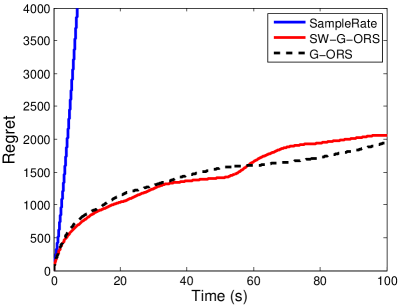
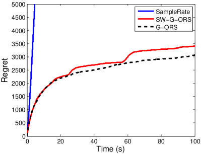
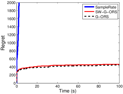
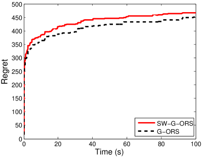
We first consider 802.11g with 8 available rates from 6 to 54 Mbit/s. Algorithms are tested in three different scenarios as in [4]: steep, gradual, and lossy. In steep scenarios, the successful transmission probability is either very high or very low. In gradual scenarios, the best rate is the highest rate with success probability higher than 0.5. Finally in lossy scenarios, the best rate has a low success probability, i.e., less than 0.5. In stationary environments, the success transmission probabilities at the various rates are (steep) θ=(.99,.98,.96,.93,0.9,.1,.06,.04)𝜃.99.98.96.930.9.1.06.04\theta=(.99,.98,.96,.93,0.9,.1,.06,.04), (gradual) θ=(.95,.9,.8,.65,.45,.25,.15,.1)𝜃.95.9.8.65.45.25.15.1\theta=(.95,.9,.8,.65,.45,.25,.15,.1), and (lossy) θ=(.9,.8,.7,.55,.45,.35,.2,.1)𝜃.9.8.7.55.45.35.2.1\theta=(.9,.8,.7,.55,.45,.35,.2,.1). Observe that in all cases, θ𝒯𝒰G𝜃𝒯subscript𝒰𝐺\theta\in{\cal T}\cap{\cal U}_{G} (unimodality holds). We compare G-ORS and SW-G-ORS to SampleRate, where the size of the sliding window is taken equal to 10s. SampleRate explores new rates every ten packet transmissions, and hence has a regret linearly increasing with time. G-ORS and SW-G-ORS explore rates in an optimal manner, and significantly outperform SampleRate as demonstrated see Fig. 3.
Refer to caption
(a) Steep
Refer to caption
(b) Steep (zoom)
Refer to caption
(c) Gradual
Refer to caption
(d) Lossy
Figure 3: Regret vs. time in stationary environments under SampleRate, G-ORS, and SW-G-ORS.

For non-stationary environments, we artificially generate varying success probabilities θ(t)𝜃𝑡\theta(t) as depicted in Fig. 4 (left). At the beginning, the value of θ𝜃\theta corresponds to a steep scenario. It then evolves to a gradual and finally lossy scenario. Fig. 4 (right) compares the performance of SW-G-ORS to that of SampleRate and of an oracle algorithm (that always knows the best rate for transmission). SW-G-ORS again outperforms SampleRate, and its performance is close to that of the Oracle algorithm (aware of the success probabilities at various rates).
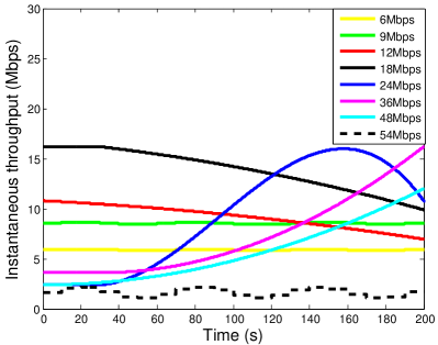
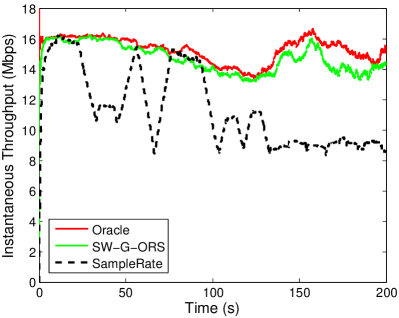
Refer to caption
Refer to caption
Figure 4: Artificially generated non-stationary environment: (left) throughput at different rates; (right) throughput (averaged over 10s) under SW-G-ORS, SampleRate, and the Oracle algorithm.

9.1.2 Test-bed traces

We now present results obtained on our 802.11g test-bed, consisting of two 802.11g nodes connected in ad-hoc mode. We collect traces recording the throughputs at the 8 available rates, and then use these traces to test SampleRate, and SW-G-ORS algorithm. Packets are of size 1500 bytes. We generate two kinds of traces: (a) when the two nodes have fixed positions, the successful packet transmission probabilities are roughly constant – we have a stationary environment; (b) the receiver is then moved (at the speed of a pedestrian), generating a non-stationary environment. The results are presented in Fig. 5. Again in both scenarios, SW-G-ORS clearly outperforms SampleRate, and exhibits a performance close that of the Oracle algorithm.
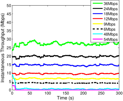
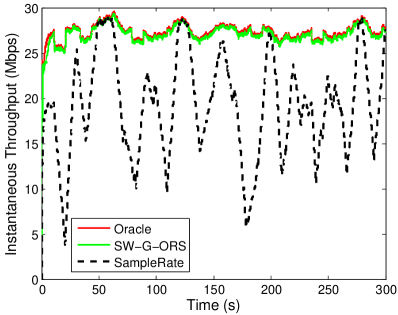
Refer to caption
Refer to caption
(a) Stationary environment
Refer to caption
Refer to caption
(b) Non-Stationary environment
Figure 5: 802.11g test-bed traces. Throughput evolution at different rates (left), and throughput under SW-G-ORS, SampleRate, and the Oracle algorithm (right) in stationary (top) and non-stationary (bottom) environment.

9.2 802.11n MIMO systems

Next we investigate the performance of SW-G-ORS in 802.11n MIMO systems with two modes, SS and DS, as in [27, 8]. We use frame aggregation (30 packets per frame) which is essential in 802.11n. SW-G-ORS is compared to MiRA [27] and SampleRate. To define SW-G-ORS, we use the graph G𝐺G depicted in Fig. 2. The sliding window for SW-G-ORS and SampleRate is taken equal to 1s. MiRA is a RA algorithm specifically designed for MIMO systems. It zigzags between MIMO modes to find the best (mode, rate) pair. In its implementation, we use, as suggested in [27], the following parameters: α=1/8𝛼18\alpha=1/8, β=1/4𝛽14\beta=1/4, and T0=0.2mssubscript𝑇00.2𝑚𝑠T_{0}=0.2ms.

Artificial traces. To generate artificial traces, we use results from [8], and more specifically, the mapping between channel measurements (the SNR and diffSNR222The maximal gap between the SNRs measured at the various antennas., see [8]) and the packet transmission success probabilities. For non-stationary scenarios, we artificially vary (smoothly) the SNR and diffSNR, and then deduce the corresponding evolution of the PER at various (mode, rate) pairs.

Test-bed traces. We also exploit real test-bed traces extracted from [8]. These traces correspond to stationary environments, and to generate real non-stationary traces, we let the system evolve between 5 stationary scenarios.

Results are presented in Fig. 6. Instantaneous throughputs are computed on a window of size 0.5s. In stationary environments, we observe, as expected, that SW-G-ORS is able to learn the best (mode, rate) pair very rapidly, faster than any other algorithm. In the tested scenarios, we find that both MiRA and SampleRate were also able to find the best pair (there are scenarios where SampleRate is not able to do it [27]). Note however that SW-G-ORS provides a better throughput than MiRA and SampleRate (these algorithms do not explore (mode, rate) pairs in an optimal way). In non-stationary scenarios, the throughput of SW-G-ORS is really close to that of the Oracle algorithm. MiRA and SampleRate do seem to be able track the best (mode, rate) pair, but the performance loss compared to SW-G-ORS can be quite significant.
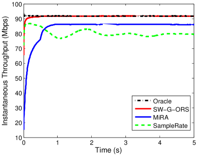
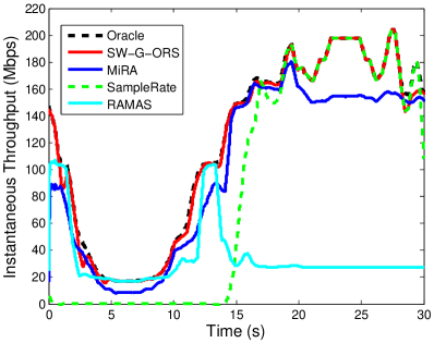
Refer to caption
Refer to caption
(a) Artificial traces
Refer to caption
Refer to caption
(b) Test-bed traces
Figure 6: Throughput under SW-G-ORS, SampleRate, MiRA, and the Oracle algorithm in 802.11n systems: (left) stationary environments, (right) non-stationary environments; (top) artificial traces, (bottom) test-bed traces.

10 Conclusion

In this paper, we investigated the fundamental limits of sampling approaches for the design of RA adaptation algorithms in 802.11 systems. We developed G-ORS, an algorithm that provably learns as fast as it is possible the best MIMO mode and rate for transmission. The proposed design methodology is based on online stochastic optimisation techniques: it is versatile, and can be easily adapted to evolving 802.11 standards. Our numerical experiments showed that G-ORS outperforms state-of-the-art sampling-based RA algorithms. This is not surprising as G-ORS is by design optimal. This performance superiority is due to the fact that under G-ORS, the way sub-optimal mode and rate pairs are explored is carefully and optimally controlled.

Appendix A Proof of Theorem 5.1

We derive here the regret lower bounds for the MAB problem (PU)subscript𝑃𝑈(P_{U}). To this aim, we apply the techniques used by Graves and Lai [13] to investigate efficient adaptive decision rules in controlled Markov chains. We recall here their general framework. Consider a controlled Markov chain (Xt)t0subscriptsubscript𝑋𝑡𝑡0(X_{t})_{t\geq 0} on a finite state space 𝒮𝒮{\cal S} with a control set U𝑈U. The transition probabilities given control uU𝑢𝑈u\in U are parametrized by θ𝜃\theta taking values in a compact metric space ΘΘ\Theta: the probability to move from state x𝑥x to state y𝑦y given the control u𝑢u and the parameter θ𝜃\theta is p(x,y;u,θ)𝑝𝑥𝑦𝑢𝜃p(x,y;u,\theta). The parameter θ𝜃\theta is not known. The decision maker is provided with a finite set of stationary control laws G={g1,,gK}𝐺subscript𝑔1subscript𝑔𝐾G=\{g_{1},\ldots,g_{K}\} where each control law gjsubscript𝑔𝑗g_{j} is a mapping from 𝒮𝒮{\cal S} to U𝑈U: when control law gjsubscript𝑔𝑗g_{j} is applied in state x𝑥x, the applied control is u=gj(x)𝑢subscript𝑔𝑗𝑥u=g_{j}(x). It is assumed that if the decision maker always selects the same control law g𝑔g the Markov chain is then irreducible with stationary distribution πθgsuperscriptsubscript𝜋𝜃𝑔\pi_{\theta}^{g}. Now the reward obtained when applying control u𝑢u in state x𝑥x is denoted by r(x,u)𝑟𝑥𝑢r(x,u), so that the expected reward achieved under control law g𝑔g is: μθ(g)=xr(x,g(x))πθg(x)subscript𝜇𝜃𝑔subscript𝑥𝑟𝑥𝑔𝑥superscriptsubscript𝜋𝜃𝑔𝑥\mu_{\theta}(g)=\sum_{x}r(x,g(x))\pi_{\theta}^{g}(x). There is an optimal control law given θ𝜃\theta whose expected reward is denoted μθargmaxgGμθ(g)superscriptsubscript𝜇𝜃subscript𝑔𝐺subscript𝜇𝜃𝑔\mu_{\theta}^{\star}\in\arg\max_{g\in G}\mu_{\theta}(g). Now the objective of the decision maker is to sequentially control laws so as to maximize the expected reward up to a given time horizon T𝑇T. As for MAB problems, the performance of a decision scheme can be quantified through the notion of regret which compares the expected reward to that obtained by always applying the optimal control law.

We now apply the above framework to our MAB problem. For (PU)subscript𝑃𝑈(P_{U}), the parameter θ𝜃\theta takes values in 𝒯𝒰𝒯𝒰{\cal T}\cap{\cal U}. The Markov chain has values in 𝒮={0,r1,,rK}𝒮0subscript𝑟1subscript𝑟𝐾{\cal S}=\{0,r_{1},\ldots,r_{K}\}. The set of control laws is G={1,,K}𝐺1𝐾G=\{1,\ldots,K\}. These laws are constant, in the sense that the control applied by control law k𝑘k does not depend on the state of the Markov chain, and corresponds to selecting rate rksubscript𝑟𝑘r_{k}. The transition probabilities are given as follows: for all x,y𝒮𝑥𝑦𝒮x,y\in{\cal S},

p(x,y;k,θ)=p(y;k,θ)={θk, if y=rk,1θk, if y=0.𝑝𝑥𝑦𝑘𝜃𝑝𝑦𝑘𝜃casessubscript𝜃𝑘 if 𝑦subscript𝑟𝑘1subscript𝜃𝑘 if 𝑦0p(x,y;k,\theta)=p(y;k,\theta)=\left\{\begin{array}[]{ll}\theta_{k},&\hbox{ if }y=r_{k},\\ 1-\theta_{k},&\hbox{ if }y=0.\end{array}\right.

Finally, the reward r(x,k)𝑟𝑥𝑘r(x,k) does not depend on the state and is equal to rkθksubscript𝑟𝑘subscript𝜃𝑘r_{k}\theta_{k}, which is also the expected reward obtained by always using control law k𝑘k.

We now fix θ𝒯𝒰𝜃𝒯𝒰\theta\in{\cal T}\cap{\cal U}. Define Ik(θ,λ)=I(θk,λk)superscript𝐼𝑘𝜃𝜆𝐼subscript𝜃𝑘subscript𝜆𝑘I^{k}(\theta,\lambda)=I(\theta_{k},\lambda_{k}) for any k𝑘k. Further define the set B(θ)𝐵𝜃B(\theta) consisting of all bad parameters λ𝒯𝒰𝜆𝒯𝒰\lambda\in{\cal T}\cap{\cal U} such that ksuperscript𝑘k^{\star} is not optimal under parameter λ𝜆\lambda, but which are statistically indistinguishable from θ𝜃\theta:

B(θ)={λ𝒯𝒰:λk=θk and maxkrkλk>rkλk},𝐵𝜃conditional-set𝜆𝒯𝒰subscript𝜆superscript𝑘subscript𝜃superscript𝑘 and subscript𝑘subscript𝑟𝑘subscript𝜆𝑘subscript𝑟superscript𝑘subscript𝜆superscript𝑘B(\theta)=\{\lambda\in{\cal T}\cap{\cal U}:\lambda_{k^{\star}}=\theta_{k^{\star}}\textrm{ and }\max_{k}r_{k}\lambda_{k}>r_{k^{\star}}\lambda_{k^{\star}}\},

B(θ)𝐵𝜃B(\theta) can be written as the union of sets Bk(θ)subscript𝐵𝑘𝜃B_{k}(\theta), k=1,,K𝑘1𝐾k=1,\ldots,K defined as:

Bk(θ)={λB(θ):rkλk>rkλk}.subscript𝐵𝑘𝜃conditional-set𝜆𝐵𝜃subscript𝑟𝑘subscript𝜆𝑘subscript𝑟superscript𝑘subscript𝜆superscript𝑘B_{k}(\theta)=\{\lambda\in B(\theta):r_{k}\lambda_{k}>r_{k^{\star}}\lambda_{k^{\star}}\}.

Note that Bk(θ)=subscript𝐵𝑘𝜃B_{k}(\theta)=\emptyset if rk<rkθksubscript𝑟𝑘subscript𝑟superscript𝑘subscript𝜃superscript𝑘r_{k}<r_{k^{\star}}\theta_{k^{\star}}. Define P={k:rkrkθk}𝑃conditional-set𝑘subscript𝑟𝑘subscript𝑟superscript𝑘subscript𝜃superscript𝑘P=\{k:r_{k}\geq r_{k^{\star}}\theta_{k^{\star}}\}. Observe that there exist k0subscript𝑘0k_{0} and k1subscript𝑘1k_{1} such that k0kk1subscript𝑘0superscript𝑘subscript𝑘1k_{0}\leq k^{\star}\leq k_{1} and P={k0,,k1}𝑃subscript𝑘0subscript𝑘1P=\{k_{0},\ldots,k_{1}\}. Further define P=P{k}superscript𝑃𝑃superscript𝑘P^{\prime}=P\setminus\{k^{\star}\}.

By applying Theorem 1 in [13], we know that c(θ)𝑐𝜃c(\theta) is the minimal value of the following LP:

min kck(rkθkrkθk)subscript𝑘subscript𝑐𝑘subscript𝑟superscript𝑘subscript𝜃superscript𝑘subscript𝑟𝑘subscript𝜃𝑘\displaystyle\sum_{k}c_{k}(r_{k^{\star}}\theta_{k^{\star}}-r_{k}\theta_{k}) (10)
s.t. infλBk(θ)lkclIl(θ,λ)1,kPformulae-sequencesubscriptinfimum𝜆subscript𝐵𝑘𝜃subscript𝑙superscript𝑘subscript𝑐𝑙superscript𝐼𝑙𝜃𝜆1for-all𝑘superscript𝑃\displaystyle\inf_{\lambda\in B_{k}(\theta)}\sum_{l\neq k^{\star}}c_{l}I^{l}(\theta,\lambda)\geq 1,\quad\forall k\in P^{\prime} (11)
ck0,k.subscript𝑐𝑘0for-all𝑘\displaystyle c_{k}\geq 0,\quad\forall k. (12)

Next we show that the constraints (11) on the cksubscript𝑐𝑘c_{k}’s are equivalent to:

minkN(k)ckI(θk,rkθkrk)1.subscript𝑘𝑁superscript𝑘subscript𝑐𝑘𝐼subscript𝜃𝑘subscript𝑟superscript𝑘subscript𝜃superscript𝑘subscript𝑟𝑘1\min_{k\in N(k^{\star})}c_{k}I(\theta_{k},{r_{k^{\star}}\theta_{k^{\star}}\over r_{k}})\geq 1. (13)

To this aim, let kP𝑘superscript𝑃k\in P^{\prime}. Without loss of generality assume that k>k𝑘superscript𝑘k>k^{\star}. We prove that:

infλBk(θ)lkclIl(θ,λ)=l=k+1kclI(θl,rkθkrl).subscriptinfimum𝜆subscript𝐵𝑘𝜃subscript𝑙superscript𝑘subscript𝑐𝑙superscript𝐼𝑙𝜃𝜆superscriptsubscript𝑙superscript𝑘1𝑘subscript𝑐𝑙𝐼subscript𝜃𝑙subscript𝑟superscript𝑘subscript𝜃superscript𝑘subscript𝑟𝑙\inf_{\lambda\in B_{k}(\theta)}\sum_{l\neq k^{\star}}c_{l}I^{l}(\theta,\lambda)=\sum_{l=k^{\star}+1}^{k}c_{l}I(\theta_{l},{r_{k^{\star}}\theta_{k^{\star}}\over r_{l}}). (14)

This is simply due to the following two observations:

  • for all λBk(θ)𝜆subscript𝐵𝑘𝜃\lambda\in B_{k}(\theta), we have λkrk=θkrksubscript𝜆superscript𝑘subscript𝑟superscript𝑘subscript𝜃superscript𝑘subscript𝑟superscript𝑘\lambda_{k^{\star}}r_{k^{\star}}=\theta_{k^{\star}}r_{k^{\star}} and λkrk>λkrksubscript𝜆𝑘subscript𝑟𝑘subscript𝜆superscript𝑘subscript𝑟superscript𝑘\lambda_{k}r_{k}>\lambda_{k^{\star}}r_{k^{\star}}, which using the unimodality of λ𝜆\lambda, implies that for any l{k,,k}𝑙superscript𝑘𝑘l\in\{k^{\star},\ldots,k\}, λlrlθkrksubscript𝜆𝑙subscript𝑟𝑙subscript𝜃superscript𝑘subscript𝑟superscript𝑘\lambda_{l}r_{l}\geq\theta_{k^{\star}}r_{k^{\star}}. Hence:

    lkclIl(θ,λ)l=k+1kclI(θl,rkθkrl).subscript𝑙superscript𝑘subscript𝑐𝑙superscript𝐼𝑙𝜃𝜆superscriptsubscript𝑙superscript𝑘1𝑘subscript𝑐𝑙𝐼subscript𝜃𝑙subscript𝑟superscript𝑘subscript𝜃superscript𝑘subscript𝑟𝑙\sum_{l\neq k^{\star}}c_{l}I^{l}(\theta,\lambda)\geq\sum_{l=k^{\star}+1}^{k}c_{l}I(\theta_{l},{r_{k^{\star}}\theta_{k^{\star}}\over r_{l}}).
  • For ϵ>0italic-ϵ0\epsilon>0, define λϵsubscript𝜆italic-ϵ\lambda_{\epsilon} as follows: for all l{k,,k}𝑙superscript𝑘𝑘l\in\{k^{\star},\ldots,k\}, λl=(1+(lk)ϵ)rkθkrlsubscript𝜆𝑙1𝑙superscript𝑘italic-ϵsubscript𝑟superscript𝑘subscript𝜃superscript𝑘subscript𝑟𝑙\lambda_{l}=(1+(l-k^{\star})\epsilon){r_{k^{\star}}\theta_{k^{\star}}\over r_{l}}, and for all l{k,,k}𝑙superscript𝑘𝑘l\notin\{k^{\star},\ldots,k\}, λl=θlsubscript𝜆𝑙subscript𝜃𝑙\lambda_{l}=\theta_{l}. By construction, λϵBk(θ)subscript𝜆italic-ϵsubscript𝐵𝑘𝜃\lambda_{\epsilon}\in B_{k}(\theta), and

    limϵ0lkclIl(θ,λϵ)=l=k+1kclI(θl,rkθkrl).subscriptitalic-ϵ0subscript𝑙superscript𝑘subscript𝑐𝑙superscript𝐼𝑙𝜃subscript𝜆italic-ϵsuperscriptsubscript𝑙superscript𝑘1𝑘subscript𝑐𝑙𝐼subscript𝜃𝑙subscript𝑟superscript𝑘subscript𝜃superscript𝑘subscript𝑟𝑙\lim_{\epsilon\to 0}\sum_{l\neq k^{\star}}c_{l}I^{l}(\theta,\lambda_{\epsilon})=\sum_{l=k^{\star}+1}^{k}c_{l}I(\theta_{l},{r_{k^{\star}}\theta_{k^{\star}}\over r_{l}}).

From (14), we deduce that constraints (11) are equivalent to (13) (indeed, only the constraints related to kN(k)𝑘𝑁superscript𝑘k\in N(k^{\star}) are really active, and for kN(k)𝑘𝑁superscript𝑘k\in N(k^{\star}), (11) is equivalent to ckI(θk,rkθkrk)1subscript𝑐𝑘𝐼subscript𝜃𝑘subscript𝑟superscript𝑘subscript𝜃superscript𝑘subscript𝑟𝑘1c_{k}I(\theta_{k},{r_{k^{\star}}\theta_{k^{\star}}\over r_{k}})\geq 1). With the constraints (13), the optimization problem becomes straightforward to solve, and its solution yields:

c(θ)=kN(k)rkθkrkθk)I(θk,rkθkrk).c(\theta)=\sum_{k\in N(k^{\star})}{r_{k^{\star}}\theta_{k^{\star}}-r_{k}\theta_{k})\over I(\theta_{k},{r_{k^{\star}}\theta_{k^{\star}}\over r_{k}})}.

\Box

Appendix B Proof of Theorem 5.2

The proof of Theorem 5.2 is similar to that of Theorem 5.1. The only difference is that in absence of correlations and unimodality, we can only assume that the parameter θ𝜃\theta takes values in [0,1]Ksuperscript01𝐾[0,1]^{K}.

In what follows, we fix θ[0,1]K𝜃superscript01𝐾\theta\in[0,1]^{K}, and denote by ksuperscript𝑘k^{\star} the index of the optimal rate. The sets B(θ)𝐵𝜃B(\theta) and Bk(θ)subscript𝐵𝑘𝜃B_{k}(\theta) are now defined as:

B(θ)={λ[0,1]K:λk=θk and maxkrkλk>rkλk}.𝐵𝜃conditional-set𝜆superscript01𝐾subscript𝜆superscript𝑘subscript𝜃superscript𝑘 and subscript𝑘subscript𝑟𝑘subscript𝜆𝑘subscript𝑟superscript𝑘subscript𝜆superscript𝑘B(\theta)=\{\lambda\in[0,1]^{K}:\lambda_{k^{\star}}=\theta_{k^{\star}}\textrm{ and }\max_{k}r_{k}\lambda_{k}>r_{k^{\star}}\lambda_{k^{\star}}\}.
Bk(θ)={λB(θ):rkλk>rkλk}.subscript𝐵𝑘𝜃conditional-set𝜆𝐵𝜃subscript𝑟𝑘subscript𝜆𝑘subscript𝑟superscript𝑘subscript𝜆superscript𝑘B_{k}(\theta)=\{\lambda\in B(\theta):r_{k}\lambda_{k}>r_{k^{\star}}\lambda_{k^{\star}}\}.

By applying Theorem 1 in [13], we know that c(θ)superscript𝑐𝜃c^{\prime}(\theta) is the minimal value of the following optimization problem:

min kck(rkθkrkθk)s.t. infλBk(θ)lkclIl(θ,λ)1,kkck0,k.min subscript𝑘subscript𝑐𝑘subscript𝑟superscript𝑘subscript𝜃superscript𝑘subscript𝑟𝑘subscript𝜃𝑘s.t. formulae-sequencesubscriptinfimum𝜆subscript𝐵𝑘𝜃subscript𝑙superscript𝑘subscript𝑐𝑙superscript𝐼𝑙𝜃𝜆1for-all𝑘superscript𝑘missing-subexpressionsubscript𝑐𝑘0for-all𝑘\displaystyle\begin{array}[]{ll}\textrm{min }&\sum_{k}c_{k}(r_{k^{\star}}\theta_{k^{\star}}-r_{k}\theta_{k})\\ \textrm{s.t. }&\inf_{\lambda\in B_{k}(\theta)}\sum_{l\neq k^{\star}}c_{l}I^{l}(\theta,\lambda)\geq 1,\quad\forall k\neq k^{\star}\\ &c_{k}\geq 0,\quad\forall k.\end{array}

We now solve : infλBk(θ)lkclIl(θ,λ).subscriptinfimum𝜆subscript𝐵𝑘𝜃subscript𝑙superscript𝑘subscript𝑐𝑙superscript𝐼𝑙𝜃𝜆\inf_{\lambda\in B_{k}(\theta)}\sum_{l\neq k^{\star}}c_{l}I^{l}(\theta,\lambda). Remark that for k<k0𝑘subscript𝑘0k<k_{0}, Bk(θ)=subscript𝐵𝑘𝜃B_{k}(\theta)=\emptyset, because rkθk>rksubscript𝑟superscript𝑘subscript𝜃superscript𝑘subscript𝑟𝑘r_{k^{\star}}\theta_{k^{\star}}>r_{k} for k<k0𝑘subscript𝑘0k<k_{0}. Let kk0𝑘subscript𝑘0k\geq k_{0}. For any fixed θ𝜃\theta and all l𝑙l,

Il(θ,λ)=θllogθlλl+(1θl)log1θl1λlsuperscript𝐼𝑙𝜃𝜆subscript𝜃𝑙subscript𝜃𝑙subscript𝜆𝑙1subscript𝜃𝑙1subscript𝜃𝑙1subscript𝜆𝑙I^{l}(\theta,\lambda)=\theta_{l}\log\frac{\theta_{l}}{\lambda_{l}}+(1-\theta_{l})\log\frac{1-\theta_{l}}{1-\lambda_{l}}

is a convex in λlsubscript𝜆𝑙\lambda_{l} and it achieves its minimum (equal to 00) at λl=θlsubscript𝜆𝑙subscript𝜃𝑙\lambda_{l}=\theta_{l}. Hence, we can choose λl=θlsubscript𝜆𝑙subscript𝜃𝑙\lambda_{l}=\theta_{l}, for all lk𝑙𝑘l\neq k. Since λBk(θ)𝜆subscript𝐵𝑘𝜃\lambda\in B_{k}(\theta), we must have λk>rkθkrksubscript𝜆𝑘subscript𝑟superscript𝑘subscript𝜃superscript𝑘subscript𝑟𝑘\lambda_{k}>\frac{r_{k^{\star}}\theta_{k^{\star}}}{r_{k}}. Hence from the convexity of I(θk,λk)𝐼subscript𝜃𝑘subscript𝜆𝑘I(\theta_{k},\lambda_{k}) in λksubscript𝜆𝑘\lambda_{k}, we get:

infλk:λk>rkθkrkI(θk,λk)=I(θk,rkθkrk).subscriptinfimum:subscript𝜆𝑘subscript𝜆𝑘subscript𝑟superscript𝑘subscript𝜃superscript𝑘subscript𝑟𝑘𝐼subscript𝜃𝑘subscript𝜆𝑘𝐼subscript𝜃𝑘subscript𝑟superscript𝑘subscript𝜃superscript𝑘subscript𝑟𝑘\inf_{\lambda_{k}:\lambda_{k}>\frac{r_{k^{\star}}\theta_{k^{\star}}}{r_{k}}}I(\theta_{k},\lambda_{k})=I(\theta_{k},\frac{r_{k^{\star}}\theta_{k^{\star}}}{r_{k}}).

We deduce that infλBk(θ)lkclIl(θ,λ)=ckI(θk,rkθkrk),subscriptinfimum𝜆subscript𝐵𝑘𝜃subscript𝑙superscript𝑘subscript𝑐𝑙superscript𝐼𝑙𝜃𝜆subscript𝑐𝑘𝐼subscript𝜃𝑘subscript𝑟superscript𝑘subscript𝜃superscript𝑘subscript𝑟𝑘\inf_{\lambda\in B_{k}(\theta)}\sum_{l\neq k^{\star}}c_{l}I^{l}(\theta,\lambda)=c_{k}I(\theta_{k},\frac{r_{k^{\star}}\theta_{k^{\star}}}{r_{k}}), where the infimum is reached for λ=(θ1,,θk1,rkθkrk,θk+1,,θK)𝜆subscript𝜃1subscript𝜃𝑘1subscript𝑟superscript𝑘subscript𝜃superscript𝑘subscript𝑟𝑘subscript𝜃𝑘1subscript𝜃𝐾\lambda=(\theta_{1},\dots,\theta_{k-1},\frac{r_{k^{\star}}\theta_{k^{\star}}}{r_{k}},\theta_{k+1},\dots,\theta_{K}). Finally we obtain that:

c(θ)=k=k0,kkKrkθkrkθkI(θk,rkθkrk).superscript𝑐𝜃superscriptsubscriptformulae-sequence𝑘subscript𝑘0𝑘superscript𝑘𝐾subscript𝑟superscript𝑘subscript𝜃superscript𝑘subscript𝑟𝑘subscript𝜃𝑘𝐼subscript𝜃𝑘subscript𝑟superscript𝑘subscript𝜃superscript𝑘subscript𝑟𝑘c^{\prime}(\theta)=\sum_{k=k_{0},k\neq k^{\star}}^{K}{r_{k^{\star}}\theta_{k^{\star}}-r_{k}\theta_{k}\over I(\theta_{k},\frac{r_{k^{\star}}\theta_{k^{\star}}}{r_{k}})}.

Appendix C Proof of Theorem 6.1

Notations. Throughout the proof, by a slight abuse of notation, we omit the floor/ceiling functions when it does not create ambiguity. Consider a suboptimal rate kk𝑘superscript𝑘k\neq k^{\star}. If k𝑘k has only one neighbor, we denote it by k2subscript𝑘2{k}_{2} and we must have θkrk<θk2rk2subscript𝜃𝑘subscript𝑟𝑘subscript𝜃subscript𝑘2subscript𝑟subscript𝑘2\theta_{k}r_{k}<\theta_{{k}_{2}}r_{{k}_{2}} since k𝑘k is suboptimal. Otherwise we denote by k1subscript𝑘1{k}_{1} and k2subscript𝑘2{k}_{2} the neighbors of k𝑘k with θk1rk1<θkrk<θk2rk2subscript𝜃subscript𝑘1subscript𝑟subscript𝑘1subscript𝜃𝑘subscript𝑟𝑘subscript𝜃subscript𝑘2subscript𝑟subscript𝑘2\theta_{{k}_{1}}r_{{k}_{1}}<\theta_{k}r_{k}<\theta_{{k}_{2}}r_{{k}_{2}}.

Define the difference between the average reward of k𝑘k and ksuperscript𝑘k^{\prime} : Δk,k=|θkrkθkrk|>0subscriptΔ𝑘superscript𝑘subscript𝜃superscript𝑘subscript𝑟superscript𝑘subscript𝜃𝑘subscript𝑟𝑘0\Delta_{k,k^{\prime}}=|\theta_{k^{\prime}}r_{k^{\prime}}-\theta_{k}r_{k}|>0. We use the notation:

tk,k(n)=n=1n𝟙{L(n)=k,k(n)=k}.subscript𝑡𝑘superscript𝑘𝑛superscriptsubscriptsuperscript𝑛1𝑛1formulae-sequence𝐿𝑛𝑘𝑘𝑛superscript𝑘t_{k,k^{\prime}}(n)=\sum_{n^{\prime}=1}^{n}\mathbbm{1}\{L(n)=k,k(n)=k^{\prime}\}.

tk,k(n)subscript𝑡𝑘superscript𝑘𝑛t_{k,k^{\prime}}(n) is the number of times up time n𝑛n that ksuperscript𝑘k^{\prime} has been selected given that k𝑘k was the leader.

Proof. Let T>0𝑇0T>0. The regret RORS(T)superscript𝑅𝑂𝑅𝑆𝑇R^{ORS}(T) of ORS algorithm up to time T𝑇T is:

RORS(T)=kk(rkθkrkθk)𝔼[n=1T𝟙{k(n)=k}].superscript𝑅𝑂𝑅𝑆𝑇subscript𝑘superscript𝑘subscript𝑟superscript𝑘subscript𝜃superscript𝑘subscript𝑟𝑘subscript𝜃𝑘𝔼delimited-[]superscriptsubscript𝑛1𝑇1𝑘𝑛𝑘R^{ORS}(T)=\sum_{k\neq k^{\star}}(r_{k^{\star}}\theta_{k^{\star}}-r_{k}\theta_{k})\mathbb{E}[\sum_{n=1}^{T}\mathbbm{1}\{k(n)=k\}].

We use the following decomposition:

𝟙{k(n)=k}=𝟙{L(n)=k,k(n)=k}+𝟙{L(n)k,k(n)=k}.1𝑘𝑛𝑘1formulae-sequence𝐿𝑛superscript𝑘𝑘𝑛𝑘1formulae-sequence𝐿𝑛superscript𝑘𝑘𝑛𝑘\mathbbm{1}\{k(n)=k\}=\mathbbm{1}\{L(n)=k^{\star},k(n)=k\}+\mathbbm{1}\{L(n)\neq k^{\star},k(n)=k\}.

Now

kk(rkθkrkθk)subscript𝑘superscript𝑘subscript𝑟superscript𝑘subscript𝜃superscript𝑘subscript𝑟𝑘subscript𝜃𝑘\displaystyle\sum_{k\neq k^{\star}}(r_{k^{\star}}\theta_{k^{\star}}-r_{k}\theta_{k}) 𝔼[n=1T𝟙{L(n)k,k(n)=k}]𝔼delimited-[]superscriptsubscript𝑛1𝑇1formulae-sequence𝐿𝑛superscript𝑘𝑘𝑛𝑘\displaystyle\mathbb{E}[\sum_{n=1}^{T}\mathbbm{1}\{L(n)\neq k^{\star},k(n)=k\}]
rkkk𝔼[n=1T𝟙{L(n)k,k(n)=k}]absentsubscript𝑟superscript𝑘subscript𝑘superscript𝑘𝔼delimited-[]superscriptsubscript𝑛1𝑇1formulae-sequence𝐿𝑛superscript𝑘𝑘𝑛𝑘\displaystyle\leq r_{k^{\star}}\sum_{k\neq k^{\star}}\mathbb{E}[\sum_{n=1}^{T}\mathbbm{1}\{L(n)\neq k^{\star},k(n)=k\}]
rkkk𝔼[lk(T)].absentsubscript𝑟superscript𝑘subscript𝑘superscript𝑘𝔼delimited-[]subscript𝑙𝑘𝑇\displaystyle\leq r_{k^{\star}}\sum_{k\neq k^{\star}}\mathbb{E}[l_{k}(T)].

Observing that when L(n)=k𝐿𝑛superscript𝑘L(n)=k^{\star}, the algorithm selects a decision k𝒩(k)𝑘𝒩superscript𝑘k\in{\cal N}(k^{\star}), we deduce that:

RORS(T)rkkk𝔼[lk(T)]+kN(k)(rkθkrkθk)𝔼[n=1T𝟙{L(n)=k,k(n)=k}]superscript𝑅𝑂𝑅𝑆𝑇subscript𝑟superscript𝑘subscript𝑘superscript𝑘𝔼delimited-[]subscript𝑙𝑘𝑇subscript𝑘𝑁superscript𝑘subscript𝑟superscript𝑘subscript𝜃superscript𝑘subscript𝑟𝑘subscript𝜃𝑘𝔼delimited-[]superscriptsubscript𝑛1𝑇1formulae-sequence𝐿𝑛superscript𝑘𝑘𝑛𝑘\displaystyle R^{ORS}(T)\leq r_{k^{\star}}\sum_{k\neq k^{\star}}\mathbb{E}[l_{k}(T)]+\sum_{k\in N(k^{\star})}(r_{k^{\star}}\theta_{k^{\star}}-r_{k}\theta_{k})\mathbb{E}[\sum_{n=1}^{T}\mathbbm{1}\{L(n)=k^{\star},k(n)=k\}]

Then we analyze the two terms in the r.h.s. in the above inequality. The first term corresponds to the average number of times where ksuperscript𝑘k^{\star} is not the leader, while the second term represents the accumulated regret when the leader is ksuperscript𝑘k^{\star}. The following result states that the first term is O(log(log(T)))𝑂𝑇O(\log(\log(T))):

Theorem C.1

For kk𝑘superscript𝑘k\neq k^{\star}, 𝔼[lk(T)]=O(log(log(T)))𝔼delimited-[]subscript𝑙𝑘𝑇𝑂𝑇\mathbb{E}[l_{k}(T)]=O(\log(\log(T))).

From the above theorem, we conclude that the leader is ksuperscript𝑘k^{\star} except for a negligible number of instants (in expectation). When ksuperscript𝑘k^{\star} is the leader, ORS behaves as KL-R-UCB restricted to the set N(k)𝑁superscript𝑘N(k^{\star}) of possible decisions. Following the same analysis as in [10] (the analysis of KL-UCB), we can show that for all ϵ>0italic-ϵ0\epsilon>0 there are constants C17subscript𝐶17C_{1}\leq 7 , C2(ϵ)subscript𝐶2italic-ϵC_{2}(\epsilon) and β(ϵ)>0𝛽italic-ϵ0\beta(\epsilon)>0 such that:

𝔼[n=1T𝟙{L(n)=k,k(n)=k}]𝔼delimited-[]superscriptsubscript𝑛1𝑇1formulae-sequence𝐿𝑛superscript𝑘𝑘𝑛𝑘\displaystyle\mathbb{E}[\sum_{n=1}^{T}\mathbbm{1}\{L(n)=k^{\star},k(n)=k\}] 𝔼[n=1T𝟙{bk(n)bk(n)}]absent𝔼delimited-[]superscriptsubscript𝑛1𝑇1subscript𝑏𝑘𝑛subscript𝑏superscript𝑘𝑛\displaystyle\leq\mathbb{E}[\sum_{n=1}^{T}\mathbbm{1}\{b_{k}(n)\geq b_{k^{\star}}(n)\}]
(1+ϵ)log(T)I(θk,rkθkrk)+C1log(log(T))+C2(ϵ)Tβ(ϵ).absent1italic-ϵ𝑇𝐼subscript𝜃𝑘subscript𝑟superscript𝑘subscript𝜃superscript𝑘subscript𝑟𝑘subscript𝐶1𝑇subscript𝐶2italic-ϵsuperscript𝑇𝛽italic-ϵ\displaystyle\leq(1+\epsilon)\frac{\log(T)}{I(\theta_{k},\frac{r_{k^{\star}}\theta_{k^{\star}}}{r_{k}})}+C_{1}\log(\log(T))+\frac{C_{2}(\epsilon)}{T^{\beta(\epsilon)}}. (16)

Combining the above bound with Theorem C.1, we get:

RORS(T)superscript𝑅𝑂𝑅𝑆𝑇\displaystyle R^{ORS}(T) (1+ϵ)c(θ)log(T)+O(log(log(T))),absent1italic-ϵ𝑐𝜃𝑇𝑂𝑇\displaystyle\leq(1+\epsilon)c(\theta)\log(T)+O(\log(\log(T))), (17)

which concludes the proof of Theorem 6.1. \Box

It remains to show that Theorem C.1 holds, which is done in the next section.

Appendix D Proof of Theorem C.1

The proof of Theorem C.1 is technical, and requires a few preliminary results presented in D.1, D.2, and D.3. The theorem itself is proved in D.4.

D.1 Concentration inequalities

We recall the Hoeffding’s inequality which is used throughout the proofs.

Lemma D.1

[Hoeffding’s inequality] Let {Zt}1tnsubscriptsubscript𝑍𝑡1𝑡𝑛\{Z_{t}\}_{1\leq t\leq n} be a sequence of independent random variables with, for any t𝑡t, Zt[at,bt]subscript𝑍𝑡subscript𝑎𝑡subscript𝑏𝑡Z_{t}\in[a_{t},b_{t}] almost surely. We have, for any δ>0𝛿0\delta>0:

[|t=1n(Zt𝔼[Zt])|δ]2exp(2δ2t=1n(btat)2).delimited-[]superscriptsubscript𝑡1𝑛subscript𝑍𝑡𝔼delimited-[]subscript𝑍𝑡𝛿22superscript𝛿2superscriptsubscript𝑡1𝑛superscriptsubscript𝑏𝑡subscript𝑎𝑡2\mathbb{P}\bigg{[}\big{|}\sum_{t=1}^{n}(Z_{t}-\mathbb{E}[Z_{t}])\big{|}\geq\delta\bigg{]}\leq 2\exp\left(-\frac{2\delta^{2}}{\sum_{t=1}^{n}(b_{t}-a_{t})^{2}}\right).

We also prove a concentration inequality of independent interest for sums of bounded independent variables with a random number of summands. Lemma D.2 is not a simple consequence of Hoeffding’s inequality.

Lemma D.2

Let {Zt}tsubscriptsubscript𝑍𝑡𝑡\{Z_{t}\}_{t\in\mathbb{Z}} be a sequence of independent random variables with values in [0,B]0𝐵[0,B]. Define nsubscript𝑛{\cal F}_{n} the σ𝜎\sigma-algebra generated by {Zt}tnsubscriptsubscript𝑍𝑡𝑡𝑛\{Z_{t}\}_{t\leq n} and the filtration =(n)nsubscriptsubscript𝑛𝑛{\cal F}=({\cal F}_{n})_{n\in\mathbb{Z}}. Consider s𝑠s\in\mathbb{N}, n0subscript𝑛0n_{0}\in\mathbb{Z} and Tn0𝑇subscript𝑛0T\geq n_{0}. We define Sn=t=n0nBt(Zt𝔼[Zt])subscript𝑆𝑛superscriptsubscript𝑡subscript𝑛0𝑛subscript𝐵𝑡subscript𝑍𝑡𝔼delimited-[]subscript𝑍𝑡S_{n}=\sum_{t=n_{0}}^{n}B_{t}(Z_{t}-\mathbb{E}[Z_{t}]), where Bt{0,1}subscript𝐵𝑡01B_{t}\in\{0,1\} is a t1subscript𝑡1{\cal F}_{t-1}-measurable random variable. Further define tn=t=n0nBtsubscript𝑡𝑛superscriptsubscript𝑡subscript𝑛0𝑛subscript𝐵𝑡t_{n}=\sum_{t=n_{0}}^{n}B_{t}. Define ϕ{n0,,T+1}italic-ϕsubscript𝑛0𝑇1\phi\in\{n_{0},\dots,T+1\} a {\cal F}-stopping time such that either tϕssubscript𝑡italic-ϕ𝑠t_{\phi}\geq s or ϕ=T+1italic-ϕ𝑇1\phi=T+1.

Then we have that:

[Sϕtϕδ,ϕT]exp(2sδ2B2).delimited-[]formulae-sequencesubscript𝑆italic-ϕsubscript𝑡italic-ϕ𝛿italic-ϕ𝑇2𝑠superscript𝛿2superscript𝐵2\mathbb{P}[S_{\phi}\geq t_{\phi}\delta\;,\;\phi\leq T]\leq\exp\left(-\frac{2s\delta^{2}}{B^{2}}\right).

As a consequence:

[|Sϕ|tϕδ,ϕT]2exp(2sδ2B2).delimited-[]formulae-sequencesubscript𝑆italic-ϕsubscript𝑡italic-ϕ𝛿italic-ϕ𝑇22𝑠superscript𝛿2superscript𝐵2\mathbb{P}[|S_{\phi}|\geq t_{\phi}\delta\;,\;\phi\leq T]\leq 2\exp\left(-\frac{2s\delta^{2}}{B^{2}}\right).

Proof. Let λ>0𝜆0\lambda>0, and define Gn=exp(λ(Snδtn))𝟙{nT}subscript𝐺𝑛𝜆subscript𝑆𝑛𝛿subscript𝑡𝑛1𝑛𝑇G_{n}=\exp(\lambda(S_{n}-\delta t_{n}))\mathbbm{1}\{n\leq T\}. We have that:

[Sϕtϕδ,ϕT]delimited-[]formulae-sequencesubscript𝑆italic-ϕsubscript𝑡italic-ϕ𝛿italic-ϕ𝑇\displaystyle\mathbb{P}[S_{\phi}\geq t_{\phi}\delta\;,\;\phi\leq T] =[exp(λ(Sϕδtϕ))𝟙{ϕT}1]absentdelimited-[]𝜆subscript𝑆italic-ϕ𝛿subscript𝑡italic-ϕ1italic-ϕ𝑇1\displaystyle=\mathbb{P}[\exp(\lambda(S_{\phi}-\delta t_{\phi}))\mathbbm{1}\{\phi\leq T\}\geq 1]
=[Gϕ1]𝔼[Gϕ].absentdelimited-[]subscript𝐺italic-ϕ1𝔼delimited-[]subscript𝐺italic-ϕ\displaystyle=\mathbb{P}[G_{\phi}\geq 1]\leq\mathbb{E}[G_{\phi}].

Next we provide an upper bound 𝔼[Gϕ]𝔼delimited-[]subscript𝐺italic-ϕ\mathbb{E}[G_{\phi}]. We define the following quantities:

Ytsubscript𝑌𝑡\displaystyle Y_{t} =Bt[λ(Zt𝔼[Zt])λ2B2/8]absentsubscript𝐵𝑡delimited-[]𝜆subscript𝑍𝑡𝔼delimited-[]subscript𝑍𝑡superscript𝜆2superscript𝐵28\displaystyle=B_{t}[\lambda(Z_{t}-\mathbb{E}[Z_{t}])-\lambda^{2}B^{2}/8]
G~nsubscript~𝐺𝑛\displaystyle\tilde{G}_{n} =exp(t=n0nYt)𝟙{nT}.absentsuperscriptsubscript𝑡subscript𝑛0𝑛subscript𝑌𝑡1𝑛𝑇\displaystyle=\exp\left(\sum_{t=n_{0}}^{n}Y_{t}\right)\mathbbm{1}\{n\leq T\}.

So that G𝐺G can be written:

Gn=G~nexp(tn(λδλ2B2/8)).subscript𝐺𝑛subscript~𝐺𝑛subscript𝑡𝑛𝜆𝛿superscript𝜆2superscript𝐵28G_{n}=\tilde{G}_{n}\exp(-t_{n}(\lambda\delta-\lambda^{2}B^{2}/8)).

Setting λ=4δ/B2𝜆4𝛿superscript𝐵2\lambda=4\delta/B^{2}:

Gn=G~nexp(2tnδ2/B2).subscript𝐺𝑛subscript~𝐺𝑛2subscript𝑡𝑛superscript𝛿2superscript𝐵2G_{n}=\tilde{G}_{n}\exp(-2t_{n}\delta^{2}/B^{2}).

Using the fact that tϕssubscript𝑡italic-ϕ𝑠t_{\phi}\geq s if ϕTitalic-ϕ𝑇\phi\leq T, we can upper bound Gϕsubscript𝐺italic-ϕG_{\phi} by:

Gϕ=G~ϕexp(2tϕδ2/B2)G~ϕexp(2sδ2/B2).subscript𝐺italic-ϕsubscript~𝐺italic-ϕ2subscript𝑡italic-ϕsuperscript𝛿2superscript𝐵2subscript~𝐺italic-ϕ2𝑠superscript𝛿2superscript𝐵2G_{\phi}=\tilde{G}_{\phi}\exp(-2t_{\phi}\delta^{2}/B^{2})\leq\tilde{G}_{\phi}\exp(-2s\delta^{2}/B^{2}).

It is noted that the above inequality holds even when ϕ=T+1italic-ϕ𝑇1\phi=T+1, since GT+1=G~T+1=0subscript𝐺𝑇1subscript~𝐺𝑇10G_{T+1}=\tilde{G}_{T+1}=0. Hence:

𝔼[Gϕ]𝔼[G~ϕ]exp(2sδ2/B2).𝔼delimited-[]subscript𝐺italic-ϕ𝔼delimited-[]subscript~𝐺italic-ϕ2𝑠superscript𝛿2superscript𝐵2\mathbb{E}[G_{\phi}]\leq\mathbb{E}[\tilde{G}_{\phi}]\exp(-2s\delta^{2}/B^{2}).

We prove that (G~n)nsubscriptsubscript~𝐺𝑛𝑛(\tilde{G}_{n})_{n} is a super-martingale. We have that 𝔼[G~T+1|T]=0G~T𝔼delimited-[]conditionalsubscript~𝐺𝑇1subscript𝑇0subscript~𝐺𝑇\mathbb{E}[\tilde{G}_{T+1}|{\cal F}_{T}]=0\leq\tilde{G}_{T}. For nT1𝑛𝑇1n\leq T-1, since Bn+1subscript𝐵𝑛1B_{n+1} is nsubscript𝑛{\cal F}_{n} measurable:

𝔼[G~n+1|n]=G~n((1Bn+1)+Bn+1𝔼[exp(Yn+1)]).𝔼delimited-[]conditionalsubscript~𝐺𝑛1subscript𝑛subscript~𝐺𝑛1subscript𝐵𝑛1subscript𝐵𝑛1𝔼delimited-[]subscript𝑌𝑛1\mathbb{E}[\tilde{G}_{n+1}|{\cal F}_{n}]=\tilde{G}_{n}((1-B_{n+1})+B_{n+1}\mathbb{E}[\exp(Y_{n+1})]).

As proven by Hoeffding ([16][eq. 4.16]) since Zn+1[0,B]subscript𝑍𝑛10𝐵Z_{n+1}\in[0,B]:

𝔼[exp(λ(Zn+1𝔼[Zn+1]))]exp(λ2B2/8),𝔼delimited-[]𝜆subscript𝑍𝑛1𝔼delimited-[]subscript𝑍𝑛1superscript𝜆2superscript𝐵28\mathbb{E}[\exp(\lambda(Z_{n+1}-\mathbb{E}[Z_{n+1}]))]\leq\exp(\lambda^{2}B^{2}/8),

so 𝔼[exp(Yn+1)]1𝔼delimited-[]subscript𝑌𝑛11\mathbb{E}[\exp(Y_{n+1})]\leq 1 and (G~n)nsubscriptsubscript~𝐺𝑛𝑛(\tilde{G}_{n})_{n} is indeed a supermartingale: 𝔼[G~n+1|n]G~n𝔼delimited-[]conditionalsubscript~𝐺𝑛1subscript𝑛subscript~𝐺𝑛\mathbb{E}[\tilde{G}_{n+1}|{\cal F}_{n}]\leq\tilde{G}_{n}. Since ϕT+1italic-ϕ𝑇1\phi\leq T+1 almost surely, and (G~n)nsubscriptsubscript~𝐺𝑛𝑛(\tilde{G}_{n})_{n} is a supermartingale, Doob’s optional stopping theorem yields: 𝔼[G~ϕ]𝔼[G~n01]=1𝔼delimited-[]subscript~𝐺italic-ϕ𝔼delimited-[]subscript~𝐺subscript𝑛011\mathbb{E}[\tilde{G}_{\phi}]\leq\mathbb{E}[\tilde{G}_{n_{0}-1}]=1, and so

[Sϕtϕδ,ϕT]𝔼[Gϕ]𝔼[G~ϕ]exp(2sδ2/B2)exp(2sδ2/B2).delimited-[]formulae-sequencesubscript𝑆italic-ϕsubscript𝑡italic-ϕ𝛿italic-ϕ𝑇𝔼delimited-[]subscript𝐺italic-ϕ𝔼delimited-[]subscript~𝐺italic-ϕ2𝑠superscript𝛿2superscript𝐵22𝑠superscript𝛿2superscript𝐵2\mathbb{P}[S_{\phi}\geq t_{\phi}\delta,\phi\leq T]\leq\mathbb{E}[G_{\phi}]\leq\mathbb{E}[\tilde{G}_{\phi}]\exp(-2s\delta^{2}/B^{2})\leq\exp(-2s\delta^{2}/B^{2}).

which concludes the proof. The second inequality is obtained by symmetry.

\Box

D.2 Deviation bounds

The following two lemmas are used repeatedly in the proof of Theorem C.1. They are corollaries of Lemma D.2 and allow us to show that certain families of events happen only rarely (in expectation).

Lemma D.3 states that if a set of instants ΛΛ\Lambda can be decomposed into a family of subsets (Λ(s))s1subscriptΛ𝑠𝑠1(\Lambda(s))_{s\geq 1} of instants (each subset has at most one instant) where k𝑘k is tried sufficiently many times (tk(n)ϵssubscript𝑡𝑘𝑛italic-ϵ𝑠t_{k}(n)\geq\epsilon s, for nΛ(s)𝑛Λ𝑠n\in\Lambda(s)), then the expected number of instants in ΛΛ\Lambda at which the average reward of k𝑘k is badly estimated is finite.

Lemma D.3

Let k{1,,K}𝑘1𝐾k\in\{1,\ldots,K\}, and ϵ>0italic-ϵ0\epsilon>0. Define nsubscript𝑛{\cal F}_{n} the σ𝜎\sigma-algebra generated by (Xk(t))1tn,1kKsubscriptsubscript𝑋𝑘𝑡formulae-sequence1𝑡𝑛1𝑘𝐾(X_{k}(t))_{1\leq t\leq n,1\leq k\leq K}. Let ΛΛ\Lambda\subset\mathbb{N} be a (random) set of instants. Assume that there exists a sequence of (random) sets (Λ(s))s1subscriptΛ𝑠𝑠1(\Lambda(s))_{s\geq 1} such that (i) Λs1Λ(s)Λsubscript𝑠1Λ𝑠\Lambda\subset\cup_{s\geq 1}\Lambda(s), (ii) for all s1𝑠1s\geq 1 and all nΛ(s)𝑛Λ𝑠n\in\Lambda(s), tk(n)ϵssubscript𝑡𝑘𝑛italic-ϵ𝑠t_{k}(n)\geq\epsilon s, (iii) |Λ(s)|1Λ𝑠1|\Lambda(s)|\leq 1, and (iv) the event nΛ(s)𝑛Λ𝑠n\in\Lambda(s) is nsubscript𝑛{\cal F}_{n}-measurable. Then for all δ>0𝛿0\delta>0:

𝔼[n1𝟙{nΛ,|μ^k(n)𝔼[μ^k(n)]|>δ}]rk2ϵδ2.𝔼delimited-[]subscript𝑛11formulae-sequence𝑛Λsubscript^𝜇𝑘𝑛𝔼delimited-[]subscript^𝜇𝑘𝑛𝛿superscriptsubscript𝑟𝑘2italic-ϵsuperscript𝛿2\mathbb{E}[\sum_{n\geq 1}\mathbbm{1}\{n\in\Lambda,|\hat{\mu}_{k}(n)-\mathbb{E}[\hat{\mu}_{k}(n)]|>\delta\}]\leq\frac{r_{k}^{2}}{\epsilon\delta^{2}}. (18)

Proof. Let T1𝑇1T\geq 1. For all s1𝑠1s\geq 1, since Λ(s)Λ𝑠\Lambda(s) has at most one element, define ϕs=T+1subscriptitalic-ϕ𝑠𝑇1\phi_{s}=T+1 if Λ(s){1,,T}Λ𝑠1𝑇\Lambda(s)\cap\{1,\dots,T\} is empty and {ϕs}=Λ(s)subscriptitalic-ϕ𝑠Λ𝑠\{\phi_{s}\}=\Lambda(s) otherwise. Since Λs1Λ(s)Λsubscript𝑠1Λ𝑠\Lambda\subset\cup_{s\geq 1}\Lambda(s), we have:

n=1T𝟙{nΛ,|μ^k(n)𝔼[μ^k(n)]|>δ}s1𝟙{|μ^k(ϕs)𝔼[μ^k(ϕs)]|>δ,ϕsT}.superscriptsubscript𝑛1𝑇1formulae-sequence𝑛Λsubscript^𝜇𝑘𝑛𝔼delimited-[]subscript^𝜇𝑘𝑛𝛿subscript𝑠11formulae-sequencesubscript^𝜇𝑘subscriptitalic-ϕ𝑠𝔼delimited-[]subscript^𝜇𝑘subscriptitalic-ϕ𝑠𝛿subscriptitalic-ϕ𝑠𝑇\sum_{n=1}^{T}\mathbbm{1}\{n\in\Lambda,|\hat{\mu}_{k}(n)-\mathbb{E}[\hat{\mu}_{k}(n)]|>\delta\}\leq\sum_{s\geq 1}\mathbbm{1}\{|\hat{\mu}_{k}(\phi_{s})-\mathbb{E}[\hat{\mu}_{k}(\phi_{s})]|>\delta,\phi_{s}\leq T\}.

Taking expectations:

𝔼[n=1T𝟙{nΛ,|μ^k(n)𝔼[μ^k(n)]|>δ}]s1[|μ^k(ϕs)𝔼[μ^k(ϕs)]|>δ,ϕsT].𝔼delimited-[]superscriptsubscript𝑛1𝑇1formulae-sequence𝑛Λsubscript^𝜇𝑘𝑛𝔼delimited-[]subscript^𝜇𝑘𝑛𝛿subscript𝑠1delimited-[]formulae-sequencesubscript^𝜇𝑘subscriptitalic-ϕ𝑠𝔼delimited-[]subscript^𝜇𝑘subscriptitalic-ϕ𝑠𝛿subscriptitalic-ϕ𝑠𝑇\mathbb{E}[\sum_{n=1}^{T}\mathbbm{1}\{n\in\Lambda,|\hat{\mu}_{k}(n)-\mathbb{E}[\hat{\mu}_{k}(n)]|>\delta\}]\leq\sum_{s\geq 1}\mathbb{P}[|\hat{\mu}_{k}(\phi_{s})-\mathbb{E}[\hat{\mu}_{k}(\phi_{s})]|>\delta,\phi_{s}\leq T].

Since ϕssubscriptitalic-ϕ𝑠\phi_{s} is a stopping time upper bounded by T+1𝑇1T+1, and that tk(ϕs)ϵssubscript𝑡𝑘subscriptitalic-ϕ𝑠italic-ϵ𝑠t_{k}(\phi_{s})\geq\epsilon s we can apply Lemma D.2 to obtain:

𝔼[n=1T𝟙{nΛ,|μ^k(n)𝔼[μ^k(n)]|>δ}]s12exp(2sϵδ2rk2)rk2ϵδ2.𝔼delimited-[]superscriptsubscript𝑛1𝑇1formulae-sequence𝑛Λsubscript^𝜇𝑘𝑛𝔼delimited-[]subscript^𝜇𝑘𝑛𝛿subscript𝑠122𝑠italic-ϵsuperscript𝛿2superscriptsubscript𝑟𝑘2superscriptsubscript𝑟𝑘2italic-ϵsuperscript𝛿2\mathbb{E}[\sum_{n=1}^{T}\mathbbm{1}\{n\in\Lambda,|\hat{\mu}_{k}(n)-\mathbb{E}[\hat{\mu}_{k}(n)]|>\delta\}]\leq\sum_{s\geq 1}2\exp\left(-\frac{2s\epsilon\delta^{2}}{r_{k}^{2}}\right)\leq\frac{r_{k}^{2}}{\epsilon\delta^{2}}.

We have used the inequality: s1esw0+euw𝑑u=1/wsubscript𝑠1superscript𝑒𝑠𝑤superscriptsubscript0superscript𝑒𝑢𝑤differential-d𝑢1𝑤\sum_{s\geq 1}e^{-sw}\leq\int_{0}^{+\infty}e^{-uw}du=1/w. Since the above reasoning is valid for all T𝑇T, we obtain the claim (18). \Box

A useful corollary of Lemma D.3 is obtained by choosing δ=Δk,k/2𝛿subscriptΔ𝑘superscript𝑘2\delta=\Delta_{k,k^{\prime}}/2, when arms k𝑘k and ksuperscript𝑘k^{\prime} are separated by at least Δk,ksubscriptΔ𝑘superscript𝑘\Delta_{k,k^{\prime}}.

Lemma D.4

Let k,k{1,,K}𝑘superscript𝑘1𝐾k,k^{\prime}\in\{1,\ldots,K\} with kk𝑘superscript𝑘k\neq k^{\prime} and ϵ>0italic-ϵ0\epsilon>0. Define nsubscript𝑛{\cal F}_{n} the σ𝜎\sigma-algebra generated by (Xk(i))1in,1kKsubscriptsubscript𝑋𝑘𝑖formulae-sequence1𝑖𝑛1𝑘𝐾(X_{k}(i))_{1\leq i\leq n,1\leq k\leq K}. Let ΛΛ\Lambda\subset\mathbb{N} be a (random) set of instants. Assume that there exists a sequence of (random) sets (Λ(s))s1subscriptΛ𝑠𝑠1(\Lambda(s))_{s\geq 1} such that (i) Λs1Λ(s)Λsubscript𝑠1Λ𝑠\Lambda\subset\cup_{s\geq 1}\Lambda(s), (ii) for all s1𝑠1s\geq 1 and all nΛ(s)𝑛Λ𝑠n\in\Lambda(s), tk(n)ϵssubscript𝑡𝑘𝑛italic-ϵ𝑠t_{k}(n)\geq\epsilon s and tk(n)ϵssubscript𝑡superscript𝑘𝑛italic-ϵ𝑠t_{k^{\prime}}(n)\geq\epsilon s, (iii) for all s𝑠s we have |Λ(s)|1Λ𝑠1|\Lambda(s)|\leq 1 almost surely and (iv) for all nΛ𝑛Λn\in\Lambda, we have 𝔼[μ^k(n)]𝔼[μ^k(n)]Δk,k𝔼delimited-[]subscript^𝜇𝑘𝑛𝔼delimited-[]subscript^𝜇superscript𝑘𝑛subscriptΔ𝑘superscript𝑘\mathbb{E}[\hat{\mu}_{k}(n)]\leq\mathbb{E}[\hat{\mu}_{k^{\prime}}(n)]-\Delta_{k,k^{\prime}} (v) the event nΛ(s)𝑛Λ𝑠n\in\Lambda(s) is nsubscript𝑛{\cal F}_{n}-measurable. Then:

𝔼[n1𝟙{nΛ,μ^k(n)>μ^k(n)}]4(rk2+rk2)ϵΔk,k2.𝔼delimited-[]subscript𝑛11formulae-sequence𝑛Λsubscript^𝜇𝑘𝑛subscript^𝜇superscript𝑘𝑛4superscriptsubscript𝑟𝑘2superscriptsubscript𝑟superscript𝑘2italic-ϵsuperscriptsubscriptΔ𝑘superscript𝑘2\mathbb{E}[\sum_{n\geq 1}\mathbbm{1}\{n\in\Lambda,\hat{\mu}_{k}(n)>\hat{\mu}_{k^{\prime}}(n)\}]\leq\frac{4(r_{k}^{2}+r_{k^{\prime}}^{2})}{\epsilon\Delta_{k,k^{\prime}}^{2}}. (19)

D.3 KL divergence

We present results related to the KL divergence that will be instrumental when manipulating indexes bk(n)subscript𝑏𝑘𝑛b_{k}(n). Lemma D.5 gives an upper and a lower bound for the KL divergence. The lower bound is Pinsker’s inequality. The upper bound is due to the fact that I(p,q)𝐼𝑝𝑞I(p,q) is convex in its second argument.

Lemma D.5

For all p,q[0,1]2𝑝𝑞superscript012p,q\in[0,1]^{2}, pq𝑝𝑞p\leq q:

2(pq)2I(p,q)(pq)2q(1q).2superscript𝑝𝑞2𝐼𝑝𝑞superscript𝑝𝑞2𝑞1𝑞2(p-q)^{2}\leq I(p,q)\leq\frac{(p-q)^{2}}{q(1-q)}. (20)

and

I(p,q)(pq)2q(1q),qp+formulae-sequencesimilar-to𝐼𝑝𝑞superscript𝑝𝑞2𝑞1𝑞𝑞superscript𝑝I(p,q)\sim\frac{(p-q)^{2}}{q(1-q)}\;,\;q\to p^{+} (21)

Proof. The lower bound is Pinsker’s inequality. For the upper bound, we have:

Iq(p,q)=qpq(1q).𝐼𝑞𝑝𝑞𝑞𝑝𝑞1𝑞\frac{\partial I}{\partial q}\left(p,q\right)=\frac{q-p}{q(1-q)}.

Since qIq(p,q)maps-to𝑞𝐼𝑞𝑝𝑞q\mapsto\frac{\partial I}{\partial q}(p,q) is increasing, the fundamental theorem of calculus gives the announced result:

I(p,q)pqIu(p,u)𝑑u(pq)2q(1q).𝐼𝑝𝑞superscriptsubscript𝑝𝑞𝐼𝑢𝑝𝑢differential-d𝑢superscript𝑝𝑞2𝑞1𝑞I(p,q)\leq\int_{p}^{q}\frac{\partial I}{\partial u}\left(p,u\right)du\leq\frac{(p-q)^{2}}{q(1-q)}.

The equivalence comes from a Taylor development of qI(p,q)𝑞𝐼𝑝𝑞q\to I(p,q) at p𝑝p, since:

Iq(p,q)|q=p=0,evaluated-at𝐼𝑞𝑝𝑞𝑞𝑝0\displaystyle\frac{\partial I}{\partial q}(p,q)|_{q=p}=0,
2Iq2(p,q)|q=p=1q(1q).evaluated-atsuperscript2𝐼superscript𝑞2𝑝𝑞𝑞𝑝1𝑞1𝑞\displaystyle\frac{\partial^{2}I}{\partial q^{2}}(p,q)|_{q=p}=\frac{1}{q(1-q)}.

\Box

Lemma D.6 is straightforward from [10][Theorem 10]. It should be observed that this result is not a direct application of Sanov’s theorem; Lemma D.6 provides sharper bounds in certain cases.

Lemma D.6

For 1tk(n)τ1subscript𝑡𝑘𝑛𝜏1\leq t_{k}(n)\leq\tau and δ>0𝛿0\delta>0, if {Xk(i)}1iτsubscriptsubscript𝑋𝑘𝑖1𝑖𝜏\{X_{k}(i)\}_{1\leq i\leq\tau} are i.i.d Bernoulli random variables with parameter θksubscript𝜃𝑘\theta_{k}, we have that:

[tk(n)I(1tk(n)i=1tk(n)Xk(i),θk)δ]2eδlog(τ)exp(δ).delimited-[]subscript𝑡𝑘𝑛𝐼1subscript𝑡𝑘𝑛superscriptsubscript𝑖1subscript𝑡𝑘𝑛subscript𝑋𝑘𝑖subscript𝜃𝑘𝛿2𝑒𝛿𝜏𝛿\mathbb{P}\left[t_{k}(n)I\left(\frac{1}{t_{k}(n)}\sum_{i=1}^{t_{k}(n)}X_{k}(i),\theta_{k}\right)\geq\delta\right]\leq 2e\lceil\delta\log(\tau)\rceil\exp(-\delta).

D.4 Proof of Theorem C.1

Let k𝑘k be the index of a suboptimal rate under. Let δ>0𝛿0\delta>0, ϵ>0italic-ϵ0\epsilon>0 small enough (we provide a more precise definition later on). To derive an upper bound of 𝔼[lk(T)]𝔼delimited-[]subscript𝑙𝑘𝑇\mathbb{E}[l_{k}(T)], we decompose the set of times where k𝑘k is the leader into the following sets:

{nT:L(n)=k}AϵBϵT,conditional-set𝑛𝑇𝐿𝑛𝑘subscript𝐴italic-ϵsuperscriptsubscript𝐵italic-ϵ𝑇\{n\leq T:L(n)=k\}\subset A_{\epsilon}\cup B_{\epsilon}^{T},

where

Aϵsubscript𝐴italic-ϵ\displaystyle A_{\epsilon} ={n:L(n)=k,tk2(n)ϵlk(n)}absentconditional-set𝑛formulae-sequence𝐿𝑛𝑘subscript𝑡subscript𝑘2𝑛italic-ϵsubscript𝑙𝑘𝑛\displaystyle=\{n:L(n)=k,t_{k_{2}}(n)\geq\epsilon l_{k}(n)\}
BϵTsuperscriptsubscript𝐵italic-ϵ𝑇\displaystyle B_{\epsilon}^{T} ={nT:L(n)=k,tk2(n)ϵlk(n)}.absentconditional-set𝑛𝑇formulae-sequence𝐿𝑛𝑘subscript𝑡subscript𝑘2𝑛italic-ϵsubscript𝑙𝑘𝑛\displaystyle=\{n\leq T:L(n)=k,t_{k_{2}}(n)\leq\epsilon l_{k}(n)\}.

Hence we have:

𝔼[lk(T)]𝔼[|Aϵ|+|BϵT|],𝔼delimited-[]subscript𝑙𝑘𝑇𝔼delimited-[]subscript𝐴italic-ϵsuperscriptsubscript𝐵italic-ϵ𝑇\mathbb{E}[l_{k}(T)]\leq\mathbb{E}\big{[}|A_{\epsilon}|+|B_{\epsilon}^{T}|\big{]},

Next we provide upper bounds of 𝔼[|Aϵ|]𝔼delimited-[]subscript𝐴italic-ϵ\mathbb{E}[|A_{\epsilon}|] and 𝔼[|BϵT|]𝔼delimited-[]superscriptsubscript𝐵italic-ϵ𝑇\mathbb{E}[|B_{\epsilon}^{T}|].

Bound on 𝔼|Aϵ|𝔼subscript𝐴italic-ϵ\mathbb{E}|A_{\epsilon}|. Let nAϵ𝑛subscript𝐴italic-ϵn\in A_{\epsilon} and assume that lk(n)=ssubscript𝑙𝑘𝑛𝑠l_{k}(n)=s. By design of the algorithm, tk(n)s/3subscript𝑡𝑘𝑛𝑠3t_{k}(n)\geq s/3. Also tk2(n)ϵlk(n)=ϵssubscript𝑡subscript𝑘2𝑛italic-ϵsubscript𝑙𝑘𝑛italic-ϵ𝑠t_{k_{2}}(n)\geq\epsilon l_{k}(n)=\epsilon s. We apply Lemma D.4 with Λ(s)={nAϵ,lk(n)=s}Λ𝑠formulae-sequence𝑛subscript𝐴italic-ϵsubscript𝑙𝑘𝑛𝑠\Lambda(s)=\{n\in A_{\epsilon},l_{k}(n)=s\}, Λ=s1Λ(s)Λsubscript𝑠1Λ𝑠\Lambda=\cup_{s\geq 1}\Lambda(s). Of course, for any s𝑠s, |Λ(s)|1Λ𝑠1|\Lambda(s)|\leq 1. We have: Aϵ={nΛ:μ^k(n)μ^k2(n)}subscript𝐴italic-ϵconditional-set𝑛Λsubscript^𝜇𝑘𝑛subscript^𝜇subscript𝑘2𝑛A_{\epsilon}=\{n\in\Lambda:\hat{\mu}_{k}(n)\geq\hat{\mu}_{k_{2}}(n)\}, since when nAϵ𝑛subscript𝐴italic-ϵn\in A_{\epsilon}, k𝑘k is the leader. Lemma D.4 can be applied with k=k2superscript𝑘subscript𝑘2k^{\prime}=k_{2}. We get: 𝔼|Aϵ|<𝔼subscript𝐴italic-ϵ\mathbb{E}|A_{\epsilon}|<\infty.

Bound on 𝔼|BϵT|𝔼superscriptsubscript𝐵italic-ϵ𝑇\mathbb{E}|B_{\epsilon}^{T}|. We introduce the following sets:

  • Cδsubscript𝐶𝛿C_{\delta} is the set of instants at which the average reward of the leader k𝑘k is badly estimated:

    Cδ={n:L(n)=k,|μ^k(n)θkrk|>δ}.subscript𝐶𝛿conditional-set𝑛formulae-sequence𝐿𝑛𝑘subscript^𝜇𝑘𝑛subscript𝜃𝑘subscript𝑟𝑘𝛿C_{\delta}=\{n:L(n)=k,|\hat{\mu}_{k}(n)-\theta_{k}r_{k}|>\delta\}.
  • Dδ=Dδ,kDδ,k1subscript𝐷𝛿subscript𝐷𝛿𝑘subscript𝐷𝛿subscript𝑘1D_{\delta}=D_{\delta,k}\cup D_{\delta,k_{1}} where Dδ,k={n:L(n)=k,k(n)=k,|μ^k(n)θkrk|>δ}subscript𝐷𝛿superscript𝑘conditional-set𝑛formulae-sequence𝐿𝑛𝑘formulae-sequence𝑘𝑛superscript𝑘subscript^𝜇superscript𝑘𝑛subscript𝜃superscript𝑘subscript𝑟superscript𝑘𝛿D_{\delta,k^{\prime}}=\{n:L(n)=k,k(n)=k^{\prime},|\hat{\mu}_{k^{\prime}}(n)-\theta_{k^{\prime}}r_{k^{\prime}}|>\delta\} is the set of instants at which k𝑘k is the leader, ksuperscript𝑘k^{\prime} is selected and the average reward of ksuperscript𝑘k^{\prime} is badly estimated.

  • ET={nT:L(n)=k,bk2(n)θk2rk2}superscript𝐸𝑇conditional-set𝑛𝑇formulae-sequence𝐿𝑛𝑘subscript𝑏subscript𝑘2𝑛subscript𝜃subscript𝑘2subscript𝑟subscript𝑘2E^{T}=\{n\leq T:L(n)=k,b_{k_{2}}(n)\leq\theta_{k_{2}}r_{k_{2}}\}, is the set of instants at which k𝑘k is the leader, and the upper confidence index bk2(n)subscript𝑏subscript𝑘2𝑛b_{k_{2}}(n) underestimates the average reward θk2rk2subscript𝜃subscript𝑘2subscript𝑟subscript𝑘2\theta_{k_{2}}r_{k_{2}}.

We first prove that |BϵT|12(|Cδ|+|Dδ|+|ET|)+O(1)superscriptsubscript𝐵italic-ϵ𝑇12subscript𝐶𝛿subscript𝐷𝛿superscript𝐸𝑇𝑂1|B_{\epsilon}^{T}|\leq 12(|C_{\delta}|+|D_{\delta}|+|E^{T}|)+O(1) as T𝑇T grows large, and then provide upper bounds on 𝔼|Cδ|𝔼subscript𝐶𝛿\mathbb{E}|C_{\delta}|, 𝔼|Dδ|𝔼subscript𝐷𝛿\mathbb{E}|D_{\delta}|, and 𝔼|ET|𝔼superscript𝐸𝑇\mathbb{E}|E^{T}|. Let nBϵT𝑛superscriptsubscript𝐵italic-ϵ𝑇n\in B_{\epsilon}^{T}. When k𝑘k is the leader, the selected decision is either k1subscript𝑘1k_{1}, or k𝑘k, or k2subscript𝑘2k_{2}, and hence:

lk(n)=tk,k1(n)+tk,k(n)+tk,k2(n),subscript𝑙𝑘𝑛subscript𝑡𝑘subscript𝑘1𝑛subscript𝑡𝑘𝑘𝑛subscript𝑡𝑘subscript𝑘2𝑛l_{k}(n)=t_{k,k_{1}}(n)+t_{k,k}(n)+t_{k,k_{2}}(n),

where recall that tk,k(n)subscript𝑡𝑘superscript𝑘𝑛t_{k,k^{\prime}}(n) denotes the number of times up to time n𝑛n when k𝑘k is the leader and ksuperscript𝑘k^{\prime} is selected. Since nBϵT𝑛superscriptsubscript𝐵italic-ϵ𝑇n\in B_{\epsilon}^{T}, tk,k2(n)ϵlk(n)subscript𝑡𝑘subscript𝑘2𝑛italic-ϵsubscript𝑙𝑘𝑛t_{k,k_{2}}(n)\leq\epsilon l_{k}(n), from which we deduce that:

(1ϵ)lk(n)tk,k1(n)+tk,k(n).1italic-ϵsubscript𝑙𝑘𝑛subscript𝑡𝑘subscript𝑘1𝑛subscript𝑡𝑘𝑘𝑛(1-\epsilon)l_{k}(n)\leq t_{k,k_{1}}(n)+t_{k,k}(n).

Choose ϵ<1/6italic-ϵ16\epsilon<1/6. With this choice, from the previous inequality, we must have that either (a) tk,k1(n)lk(n)/3subscript𝑡𝑘subscript𝑘1𝑛subscript𝑙𝑘𝑛3t_{k,k_{1}}(n)\geq l_{k}(n)/3 or (b) tk,k(n)lk(n)/2+1subscript𝑡𝑘𝑘𝑛subscript𝑙𝑘𝑛21t_{k,k}(n)\geq l_{k}(n)/2+1.

(a) Assume that tk,k1(n)lk(n)/3subscript𝑡𝑘subscript𝑘1𝑛subscript𝑙𝑘𝑛3t_{k,k_{1}}(n)\geq l_{k}(n)/3. Since tk,k1(n)subscript𝑡𝑘subscript𝑘1𝑛t_{k,k_{1}}(n) is only incremented when k1subscript𝑘1k_{1} is selected and k𝑘k is the leader, and since nlk(n)maps-to𝑛subscript𝑙𝑘𝑛n\mapsto l_{k}(n) is increasing, there exists a unique ϕ(n)<nitalic-ϕ𝑛𝑛\phi(n)<n such that L(ϕ(n))=k𝐿italic-ϕ𝑛𝑘L(\phi(n))=k, k(ϕ(n))=k1𝑘italic-ϕ𝑛subscript𝑘1k(\phi(n))=k_{1}, tk,k1(ϕ(n))=lk(n)/6subscript𝑡𝑘subscript𝑘1italic-ϕ𝑛subscript𝑙𝑘𝑛6t_{k,k_{1}}(\phi(n))=\lfloor l_{k}(n)/6\rfloor. ϕ(n)italic-ϕ𝑛\phi(n) is indeed unique because tk,k1(ϕ(n))subscript𝑡𝑘subscript𝑘1italic-ϕ𝑛t_{k,k_{1}}(\phi(n)) is incremented at time ϕ(n)italic-ϕ𝑛\phi(n).

Next we prove by contradiction that for lk(n)l0subscript𝑙𝑘𝑛subscript𝑙0l_{k}(n)\geq l_{0} large enough and δ𝛿\delta small enough, we must have ϕ(n)CδDδETitalic-ϕ𝑛subscript𝐶𝛿subscript𝐷𝛿superscript𝐸𝑇\phi(n)\in C_{\delta}\cup D_{\delta}\cup E^{T}. Assume that ϕ(n)CδDδETitalic-ϕ𝑛subscript𝐶𝛿subscript𝐷𝛿superscript𝐸𝑇\phi(n)\notin C_{\delta}\cup D_{\delta}\cup E^{T}. Then bk2(ϕ(n))θk2rk2subscript𝑏subscript𝑘2italic-ϕ𝑛subscript𝜃subscript𝑘2subscript𝑟subscript𝑘2b_{k_{2}}(\phi(n))\geq\theta_{k_{2}}r_{k_{2}}, μ^k1(ϕ(n))θk1rk1+δsubscript^𝜇subscript𝑘1italic-ϕ𝑛subscript𝜃subscript𝑘1subscript𝑟subscript𝑘1𝛿\hat{\mu}_{k_{1}}(\phi(n))\leq\theta_{k_{1}}r_{k_{1}}+\delta. Using Pinsker’s inequality and the fact that tk1(ϕ(n))tk,k1(ϕ(n))subscript𝑡subscript𝑘1italic-ϕ𝑛subscript𝑡𝑘subscript𝑘1italic-ϕ𝑛t_{k_{1}}(\phi(n))\geq t_{k,k_{1}}(\phi(n)):

bk1(ϕ(n))subscript𝑏subscript𝑘1italic-ϕ𝑛\displaystyle b_{k_{1}}(\phi(n)) μ^k1(ϕ(n))+log(lk(ϕ(n)))+clog(log(lk(ϕ(n))))2tk1(ϕ(n))absentsubscript^𝜇subscript𝑘1italic-ϕ𝑛subscript𝑙𝑘italic-ϕ𝑛𝑐subscript𝑙𝑘italic-ϕ𝑛2subscript𝑡subscript𝑘1italic-ϕ𝑛\displaystyle\leq\hat{\mu}_{k_{1}}(\phi(n))+\sqrt{\frac{\log(l_{k}(\phi(n)))+c\log(\log(l_{k}(\phi(n))))}{2t_{k_{1}}(\phi(n))}}
θk1rk1+δ+log(lk(n))+clog(log(lk(n)))2lk(n)/6.absentsubscript𝜃subscript𝑘1subscript𝑟subscript𝑘1𝛿subscript𝑙𝑘𝑛𝑐subscript𝑙𝑘𝑛2subscript𝑙𝑘𝑛6\displaystyle\leq\theta_{k_{1}}r_{k_{1}}+\delta+\sqrt{\frac{\log(l_{k}(n))+c\log(\log(l_{k}(n)))}{2\lfloor l_{k}(n)/6\rfloor}}.

Now select δ<(θk2rk2θkrk)/2𝛿subscript𝜃subscript𝑘2subscript𝑟subscript𝑘2subscript𝜃𝑘subscript𝑟𝑘2\delta<(\theta_{k_{2}}r_{k_{2}}-\theta_{k}r_{k})/2 and l0subscript𝑙0l_{0} such that (log(l0)+clog(log(l0)))/2l0/6δsubscript𝑙0𝑐subscript𝑙02subscript𝑙06𝛿\sqrt{(\log(l_{0})+c\log(\log(l_{0})))/2\lfloor l_{0}/6\rfloor}\leq\delta. If lk(n)l0subscript𝑙𝑘𝑛subscript𝑙0l_{k}(n)\geq l_{0}:

bk1(ϕ(n))θk1rk1+2δ<θk2rk2bk2(ϕ(n)),subscript𝑏subscript𝑘1italic-ϕ𝑛subscript𝜃subscript𝑘1subscript𝑟subscript𝑘12𝛿subscript𝜃subscript𝑘2subscript𝑟subscript𝑘2subscript𝑏subscript𝑘2italic-ϕ𝑛b_{k_{1}}(\phi(n))\leq\theta_{k_{1}}r_{k_{1}}+2\delta<\theta_{k_{2}}r_{k_{2}}\leq b_{k_{2}}(\phi(n)),

which implies that k1subscript𝑘1k_{1} cannot be selected at time ϕ(n)italic-ϕ𝑛\phi(n) (because bk1(ϕ(n))<bk2(ϕ(n))subscript𝑏subscript𝑘1italic-ϕ𝑛subscript𝑏subscript𝑘2italic-ϕ𝑛b_{k_{1}}(\phi(n))<b_{k_{2}}(\phi(n))), a contradiction.

(b) Assume that tk,k(n)lk(n)/2+1=lk(n)/3+lk(n)/6+1subscript𝑡𝑘𝑘𝑛subscript𝑙𝑘𝑛21subscript𝑙𝑘𝑛3subscript𝑙𝑘𝑛61t_{k,k}(n)\geq l_{k}(n)/2+1=l_{k}(n)/3+l_{k}(n)/6+1. There are at least lk(n)/6+1subscript𝑙𝑘𝑛61l_{k}(n)/6+1 instants n~~𝑛\tilde{n} such that lk(n~)1subscript𝑙𝑘~𝑛1l_{k}(\tilde{n})-1 is not a multiple of 333, L(n~)=k𝐿~𝑛𝑘L(\tilde{n})=k and k(n~)=k𝑘~𝑛𝑘k(\tilde{n})=k. By the same reasoning as in (a) there exists a unique ϕ(n)<nitalic-ϕ𝑛𝑛\phi(n)<n such that L(ϕ(n))=k𝐿italic-ϕ𝑛𝑘L(\phi(n))=k, k(ϕ(n))=k𝑘italic-ϕ𝑛𝑘k(\phi(n))=k , tk,k(ϕ(n))=lk(n)/6subscript𝑡𝑘𝑘italic-ϕ𝑛subscript𝑙𝑘𝑛6t_{k,k}(\phi(n))=\lfloor l_{k}(n)/6\rfloor and (lk(ϕ(n))1)subscript𝑙𝑘italic-ϕ𝑛1(l_{k}(\phi(n))-1) is not a multiple of 333. So bk(ϕ(n))bk2(ϕ(n))subscript𝑏𝑘italic-ϕ𝑛subscript𝑏subscript𝑘2italic-ϕ𝑛b_{k}(\phi(n))\geq b_{k_{2}}(\phi(n)). The same reasoning as that applied in (a) (replacing k1subscript𝑘1k_{1} by k𝑘k) yields ϕ(n)CδDδETitalic-ϕ𝑛subscript𝐶𝛿subscript𝐷𝛿superscript𝐸𝑇\phi(n)\in C_{\delta}\cup D_{\delta}\cup E^{T}.

We define Bϵ,l0T={n:nBϵT,lk(n)l0}superscriptsubscript𝐵italic-ϵsubscript𝑙0𝑇conditional-set𝑛formulae-sequence𝑛superscriptsubscript𝐵italic-ϵ𝑇subscript𝑙𝑘𝑛subscript𝑙0B_{\epsilon,l_{0}}^{T}=\{n:n\in B_{\epsilon}^{T},l_{k}(n)\geq l_{0}\}, and we have that |BϵT|l0+|Bϵ,l0T|superscriptsubscript𝐵italic-ϵ𝑇subscript𝑙0superscriptsubscript𝐵italic-ϵsubscript𝑙0𝑇|B_{\epsilon}^{T}|\leq l_{0}+|B_{\epsilon,l_{0}}^{T}|. We have defined a mapping ϕitalic-ϕ\phi from Bϵ,l0Tsuperscriptsubscript𝐵italic-ϵsubscript𝑙0𝑇B_{\epsilon,l_{0}}^{T} to CδDδETsubscript𝐶𝛿subscript𝐷𝛿superscript𝐸𝑇C_{\delta}\cup D_{\delta}\cup E^{T}. To bound the size of Bϵ,l0Tsuperscriptsubscript𝐵italic-ϵsubscript𝑙0𝑇B_{\epsilon,l_{0}}^{T}, we use the following decomposition:

{n:nBϵ,l0T,lk(n)l0}nCδDδET{n:nBϵ,l0T,ϕ(n)=n}.conditional-set𝑛formulae-sequence𝑛superscriptsubscript𝐵italic-ϵsubscript𝑙0𝑇subscript𝑙𝑘𝑛subscript𝑙0subscriptsuperscript𝑛subscript𝐶𝛿subscript𝐷𝛿superscript𝐸𝑇conditional-set𝑛formulae-sequence𝑛superscriptsubscript𝐵italic-ϵsubscript𝑙0𝑇italic-ϕ𝑛superscript𝑛\{n:n\in B_{\epsilon,l_{0}}^{T},l_{k}(n)\geq l_{0}\}\subset\cup_{n^{\prime}\in C_{\delta}\cup D_{\delta}\cup E^{T}}\{n:n\in B_{\epsilon,l_{0}}^{T},\phi(n)=n^{\prime}\}.

Let us fix nsuperscript𝑛n^{\prime}. If nBϵ,l0T𝑛superscriptsubscript𝐵italic-ϵsubscript𝑙0𝑇n\in B_{\epsilon,l_{0}}^{T} and ϕ(n)=nitalic-ϕ𝑛superscript𝑛\phi(n)=n^{\prime}, then lk(n)/6{tk,k1(n),tk,k(n)}subscript𝑙𝑘𝑛6subscript𝑡𝑘subscript𝑘1superscript𝑛subscript𝑡𝑘𝑘superscript𝑛\lfloor l_{k}(n)/6\rfloor\in\{t_{k,k_{1}}(n^{\prime}),t_{k,k}(n^{\prime})\} and lk(n)subscript𝑙𝑘𝑛l_{k}(n) is incremented at time n𝑛n because L(n)=k𝐿𝑛𝑘L(n)=k. Therefore:

|{n:nBϵ,l0T,ϕ(n)=n}|12.conditional-set𝑛formulae-sequence𝑛superscriptsubscript𝐵italic-ϵsubscript𝑙0𝑇italic-ϕ𝑛superscript𝑛12|\{n:n\in B_{\epsilon,l_{0}}^{T},\phi(n)=n^{\prime}\}|\leq 12.

Using union bound, we obtain the desired result:

|BϵT|l0+|Bϵ,l0T|O(1)+12(|Cδ|+|Dδ|+|ET|).superscriptsubscript𝐵italic-ϵ𝑇subscript𝑙0superscriptsubscript𝐵italic-ϵsubscript𝑙0𝑇𝑂112subscript𝐶𝛿subscript𝐷𝛿superscript𝐸𝑇|B_{\epsilon}^{T}|\leq l_{0}+|B_{\epsilon,l_{0}}^{T}|\leq O(1)+12(|C_{\delta}|+|D_{\delta}|+|E^{T}|).

Bound on 𝔼|Cδ|𝔼subscript𝐶𝛿\mathbb{E}|C_{\delta}|. We apply Lemma D.3 with Λ(s)={n:L(n)=k,lk(n)=s}Λ𝑠conditional-set𝑛formulae-sequence𝐿𝑛𝑘subscript𝑙𝑘𝑛𝑠\Lambda(s)=\{n:L(n)=k,l_{k}(n)=s\}, and Λ=s1Λ(s)Λsubscript𝑠1Λ𝑠\Lambda=\cup_{s\geq 1}\Lambda(s). Then of course, |Λ(s)|1Λ𝑠1|\Lambda(s)|\leq 1 for all s𝑠s. Moreover by design, tk(n)s/3subscript𝑡𝑘𝑛𝑠3t_{k}(n)\geq s/3 when nΛ(s)𝑛Λ𝑠n\in\Lambda(s), so we can choose any ϵ<1/3italic-ϵ13\epsilon<1/3 in Lemma D.3. Now Cδ={nΛ:|μ^k(n)θkrk|>δ}subscript𝐶𝛿conditional-set𝑛Λsubscript^𝜇𝑘𝑛subscript𝜃𝑘subscript𝑟𝑘𝛿C_{\delta}=\{n\in\Lambda:|\hat{\mu}_{k}(n)-\theta_{k}r_{k}|>\delta\}. From (18), we get 𝔼|Cδ|<𝔼subscript𝐶𝛿\mathbb{E}|C_{\delta}|<\infty.

Bound on 𝔼|Dδ|𝔼subscript𝐷𝛿\mathbb{E}|D_{\delta}|. Let k{k1,k}superscript𝑘subscript𝑘1𝑘k^{\prime}\in\{k_{1},k\}. Define for any s𝑠s, Λ(s)={n:L(n)=k,k(n)=k,tk(n)=s}Λ𝑠conditional-set𝑛formulae-sequence𝐿𝑛𝑘formulae-sequence𝑘𝑛superscript𝑘subscript𝑡superscript𝑘𝑛𝑠\Lambda(s)=\{n:L(n)=k,k(n)=k^{\prime},t_{k^{\prime}}(n)=s\}, and Λ=s1Λ(s)Λsubscript𝑠1Λ𝑠\Lambda=\cup_{s\geq 1}\Lambda(s). We have |Λ(s)|1Λ𝑠1|\Lambda(s)|\leq 1, and for any nΛ(s)𝑛Λ𝑠n\in\Lambda(s), tk(n)=sϵssubscript𝑡superscript𝑘𝑛𝑠italic-ϵ𝑠t_{k^{\prime}}(n)=s\geq\epsilon s for any ϵ<1italic-ϵ1\epsilon<1. We can now apply Lemma D.3 (where k𝑘k is replaced by ksuperscript𝑘k^{\prime}). Note that Dδ={nΛ:|μ^k(n)θkrk|>δ}subscript𝐷𝛿conditional-set𝑛Λsubscript^𝜇superscript𝑘𝑛subscript𝜃superscript𝑘subscript𝑟superscript𝑘𝛿D_{\delta}=\{n\in\Lambda:|\hat{\mu}_{k^{\prime}}(n)-\theta_{k^{\prime}}r_{k^{\prime}}|>\delta\}, and hence (18) leads to 𝔼|Dδ,k|<𝔼subscript𝐷𝛿superscript𝑘\mathbb{E}|D_{\delta,k^{\prime}}|<\infty, and thus 𝔼|Dδ|<𝔼subscript𝐷𝛿\mathbb{E}|D_{\delta}|<\infty.

Bound on 𝔼|ET|𝔼superscript𝐸𝑇\mathbb{E}|E^{T}|. We can show as in [10] (the analysis of KL-UCB) that 𝔼|ET|=O(log(log(T)))𝔼superscript𝐸𝑇𝑂𝑇\mathbb{E}|E^{T}|=O(\log(\log(T))) (more precisely, this result is a simple application of Theorem 10 in  [10]).

We have shown that 𝔼|BϵT|=O(log(log(T)))𝔼superscriptsubscript𝐵italic-ϵ𝑇𝑂𝑇\mathbb{E}|B_{\epsilon}^{T}|=O(\log(\log(T))), and hence 𝔼[lk(T)]=O(log(log(T)))𝔼delimited-[]subscript𝑙𝑘𝑇𝑂𝑇\mathbb{E}[l_{k}(T)]=O(\log(\log(T))), which concludes the proof of Theorem C.1. \Box

Appendix E Proofs for non-stationary environments

To simplify the notation, we remove the superscript τ throughout the proofs, e.g tkτ(n)superscriptsubscript𝑡𝑘𝜏𝑛t_{k}^{\tau}(n) and lkτ(n)superscriptsubscript𝑙𝑘𝜏𝑛l_{k}^{\tau}(n) are denoted by tk(n)subscript𝑡𝑘𝑛t_{k}(n) and lk(n)subscript𝑙𝑘𝑛l_{k}(n).

E.1 A lemma for sums over a sliding window

We will use Lemma E.1 repeatedly to bound the number of times some events occur over a sliding window of size τ𝜏\tau.

Lemma E.1

Let A𝐴A\subset\mathbb{N}, and τ𝜏\tau\in\mathbb{N} fixed. Define a(n)=n=nτn1𝟙{nA}𝑎𝑛superscriptsubscriptsuperscript𝑛𝑛𝜏𝑛11superscript𝑛𝐴a(n)=\sum_{n^{\prime}=n-\tau}^{n-1}\mathbbm{1}\{n^{\prime}\in A\}. Then for all T𝑇T\in\mathbb{N} and s𝑠s\in\mathbb{N} we have the inequality:

n=1T𝟙{nA,a(n)s}sT/τ.superscriptsubscript𝑛1𝑇1formulae-sequence𝑛𝐴𝑎𝑛𝑠𝑠𝑇𝜏\sum_{n=1}^{T}\mathbbm{1}\{n\in A,a(n)\leq s\}\leq s\lceil T/\tau\rceil. (22)

As a consequence, for all k{1,,K}𝑘1𝐾k\in\{1,\dots,K\}, we have:

n=1T𝟙{k(n)=k,tk(n)s}superscriptsubscript𝑛1𝑇1formulae-sequence𝑘𝑛𝑘subscript𝑡𝑘𝑛𝑠\displaystyle\sum_{n=1}^{T}\mathbbm{1}\{k(n)=k,t_{k}(n)\leq s\} sT/τ,absent𝑠𝑇𝜏\displaystyle\leq s\lceil T/\tau\rceil, (23)
n=1T𝟙{L(n)=k,lk(n)s}superscriptsubscript𝑛1𝑇1formulae-sequence𝐿𝑛𝑘subscript𝑙𝑘𝑛𝑠\displaystyle\sum_{n=1}^{T}\mathbbm{1}\{L(n)=k,l_{k}(n)\leq s\} sT/τ.absent𝑠𝑇𝜏\displaystyle\leq s\lceil T/\tau\rceil.

These inequalities are obtained by choosing A={n:k(n)=k}𝐴conditional-set𝑛𝑘𝑛𝑘A=\{n:k(n)=k\} and A={n:L(n)=k}𝐴conditional-set𝑛𝐿𝑛𝑘A=\{n:L(n)=k\} in (22).

Proof. We decompose {1,,T}1𝑇\{1,\dots,T\} into intervals of size τ𝜏\tau: {1,,τ}1𝜏\{1,\dots,\tau\} , {τ+1,,2τ}𝜏12𝜏\{\tau+1,\dots,2\tau\} etc. We have:

n=1T𝟙{nA,a(n)s}i=0T/τ1n=1τ𝟙{n+iτA,a(n+iτ)s}.superscriptsubscript𝑛1𝑇1formulae-sequence𝑛𝐴𝑎𝑛𝑠superscriptsubscript𝑖0𝑇𝜏1superscriptsubscript𝑛1𝜏1formulae-sequence𝑛𝑖𝜏𝐴𝑎𝑛𝑖𝜏𝑠\sum_{n=1}^{T}\mathbbm{1}\{n\in A,a(n)\leq s\}\leq\sum_{i=0}^{\lceil T/\tau\rceil-1}\sum_{n=1}^{\tau}\mathbbm{1}\{n+i\tau\in A,a(n+i\tau)\leq s\}. (24)

Fix i𝑖i and assume that n=1τ𝟙{n+iτA,a(n+iτ)s}>ssuperscriptsubscript𝑛1𝜏1formulae-sequence𝑛𝑖𝜏𝐴𝑎𝑛𝑖𝜏𝑠𝑠\sum_{n=1}^{\tau}\mathbbm{1}\{n+i\tau\in A,a(n+i\tau)\leq s\}>s. Then there must exist n<τsuperscript𝑛𝜏n^{\prime}<\tau such that nAsuperscript𝑛𝐴n^{\prime}\in A and n=1n𝟙{n+iτA,a(n+iτ)s}=ssuperscriptsubscript𝑛1superscript𝑛1formulae-sequence𝑛𝑖𝜏𝐴𝑎𝑛𝑖𝜏𝑠𝑠\sum_{n=1}^{n^{\prime}}\mathbbm{1}\{n+i\tau\in A,a(n+i\tau)\leq s\}=s. Since a(n+iτ)n=1n𝟙{n+iτA,a(n+iτ)s}𝑎superscript𝑛𝑖𝜏superscriptsubscript𝑛1superscript𝑛1formulae-sequence𝑛𝑖𝜏𝐴𝑎𝑛𝑖𝜏𝑠a(n^{\prime}+i\tau)\geq\sum_{n=1}^{n^{\prime}}\mathbbm{1}\{n+i\tau\in A,a(n+i\tau)\leq s\}, we have a(n+iτ)s𝑎superscript𝑛𝑖𝜏𝑠a(n^{\prime}+i\tau)\geq s. As nAsuperscript𝑛𝐴n^{\prime}\in A, we must have a(n′′+iτ)(s+1)𝑎superscript𝑛′′𝑖𝜏𝑠1a(n^{\prime\prime}+i\tau)\geq(s+1) for all n′′>nsuperscript𝑛′′superscript𝑛n^{\prime\prime}>n^{\prime} such that n′′Asuperscript𝑛′′𝐴n^{\prime\prime}\in A. So

n=1τ𝟙{n+iτA,a(n+iτ)s}=n=1n𝟙{n+iτA,a(n+iτ)s}=s,superscriptsubscript𝑛1𝜏1formulae-sequence𝑛𝑖𝜏𝐴𝑎𝑛𝑖𝜏𝑠superscriptsubscript𝑛1superscript𝑛1formulae-sequence𝑛𝑖𝜏𝐴𝑎𝑛𝑖𝜏𝑠𝑠\sum_{n=1}^{\tau}\mathbbm{1}\{n+i\tau\in A,a(n+i\tau)\leq s\}=\sum_{n=1}^{n^{\prime}}\mathbbm{1}\{n+i\tau\in A,a(n+i\tau)\leq s\}=s,

which is a contradiction. Hence, for all i𝑖i:

n=1τ𝟙{n+iτA,a(n+iτ)s}s,superscriptsubscript𝑛1𝜏1formulae-sequence𝑛𝑖𝜏𝐴𝑎𝑛𝑖𝜏𝑠𝑠\sum_{n=1}^{\tau}\mathbbm{1}\{n+i\tau\in A,a(n+i\tau)\leq s\}\leq s,

and substituting in (24) gives the desired result:

n=1T𝟙{nA,a(n)s}i=0T/τ1s=sT/τ.superscriptsubscript𝑛1𝑇1formulae-sequence𝑛𝐴𝑎𝑛𝑠superscriptsubscript𝑖0𝑇𝜏1𝑠𝑠𝑇𝜏\sum_{n=1}^{T}\mathbbm{1}\{n\in A,a(n)\leq s\}\leq\sum_{i=0}^{\lceil T/\tau\rceil-1}s=s\lceil T/\tau\rceil.

\Box

E.2 Deviation bound

We prove a deviation bound similar to that of Lemma D.3 for non-stationary environments.

Lemma E.2

Let k{1,,K}𝑘1𝐾k\in\{1,\ldots,K\}, n0subscript𝑛0n_{0}\in\mathbb{N} and ϵ>0italic-ϵ0\epsilon>0. Let ΛΛ\Lambda\subset\mathbb{N} be a (random) set of instants. Assume that there exists a sequence of (random) sets (Λ(s))s1subscriptΛ𝑠𝑠1(\Lambda(s))_{s\geq 1} such that (i) Λs1Λ(s)Λsubscript𝑠1Λ𝑠\Lambda\subset\cup_{s\geq 1}\Lambda(s), (ii) for all s1𝑠1s\geq 1 and all nΛ(s)𝑛Λ𝑠n\in\Lambda(s), tk(n)ϵssubscript𝑡𝑘𝑛italic-ϵ𝑠t_{k}(n)\geq\epsilon s, and (iii) for all s1𝑠1s\geq 1 |Λ(s)[n0,n0+τ]|1Λ𝑠subscript𝑛0subscript𝑛0𝜏1|\Lambda(s)\cap[n_{0},n_{0}+\tau]|\leq 1. Then for all δ>0𝛿0\delta>0:

𝔼[n=n0n0+τ𝟙{nΛ,|μ^k(n)𝔼[μ^k(n)]|>δ}]log(τ)rk22ϵδ2+2.𝔼delimited-[]superscriptsubscript𝑛subscript𝑛0subscript𝑛0𝜏1formulae-sequence𝑛Λsubscript^𝜇𝑘𝑛𝔼delimited-[]subscript^𝜇𝑘𝑛𝛿𝜏superscriptsubscript𝑟𝑘22italic-ϵsuperscript𝛿22\mathbb{E}[\sum_{n=n_{0}}^{n_{0}+\tau}\mathbbm{1}\{n\in\Lambda,|\hat{\mu}_{k}(n)-\mathbb{E}[\hat{\mu}_{k}(n)]|>\delta\}]\leq\frac{\log(\tau)r_{k}^{2}}{2\epsilon\delta^{2}}+2.

Proof. Fix s01subscript𝑠01s_{0}\geq 1. We use the following decomposition, depending on the value of s𝑠s with respect to s0subscript𝑠0s_{0}:

{nΛ,|μ^k(n)𝔼[μ^k(n)]|>δ}AB,formulae-sequence𝑛Λsubscript^𝜇𝑘𝑛𝔼delimited-[]subscript^𝜇𝑘𝑛𝛿𝐴𝐵\displaystyle\{n\in\Lambda,|\hat{\mu}_{k}(n)-\mathbb{E}[\hat{\mu}_{k}(n)]|>\delta\}\subset A\cup B,

where

A𝐴\displaystyle A ={n0,,n0+τ}(1ss0Λ(s)),absentsubscript𝑛0subscript𝑛0𝜏subscript1𝑠subscript𝑠0Λ𝑠\displaystyle=\{n_{0},\dots,n_{0}+\tau\}\cap(\cup_{1\leq s\leq s_{0}}\Lambda(s)),
B𝐵\displaystyle B ={n0,,n0+τ}{nss0Λ(s):|μ^k(n)𝔼[μ^k(n)]|>δ}.absentsubscript𝑛0subscript𝑛0𝜏conditional-set𝑛subscript𝑠subscript𝑠0Λ𝑠subscript^𝜇𝑘𝑛𝔼delimited-[]subscript^𝜇𝑘𝑛𝛿\displaystyle=\{n_{0},\dots,n_{0}+\tau\}\cap\{n\in\cup_{s\geq s_{0}}\Lambda(s):|\hat{\mu}_{k}(n)-\mathbb{E}[\hat{\mu}_{k}(n)]|>\delta\}.

Since for all s𝑠s, |Λ(s){n0,,n0+τ}|1Λ𝑠subscript𝑛0subscript𝑛0𝜏1|\Lambda(s)\cap\{n_{0},\dots,n_{0}+\tau\}|\leq 1, we have |A|s0𝐴subscript𝑠0|A|\leq s_{0}. The expected size of B𝐵B is upper bounded by:

E[|B|]𝐸delimited-[]𝐵\displaystyle E[|B|] n=n0n0+τ[nss0Λ(s),|μ^k(n)𝔼[μ^k(n)]|>δ]absentsuperscriptsubscript𝑛subscript𝑛0subscript𝑛0𝜏delimited-[]formulae-sequence𝑛subscript𝑠subscript𝑠0Λ𝑠subscript^𝜇𝑘𝑛𝔼delimited-[]subscript^𝜇𝑘𝑛𝛿\displaystyle\leq\sum_{n=n_{0}}^{n_{0}+\tau}\mathbb{P}[n\in\cup_{s\geq s_{0}}\Lambda(s),|\hat{\mu}_{k}(n)-\mathbb{E}[\hat{\mu}_{k}(n)]|>\delta]
n=n0n0+τ[|μ^k(n)𝔼[μ^k(n)]|>δ,tk(n)ϵs0].absentsuperscriptsubscript𝑛subscript𝑛0subscript𝑛0𝜏delimited-[]formulae-sequencesubscript^𝜇𝑘𝑛𝔼delimited-[]subscript^𝜇𝑘𝑛𝛿subscript𝑡𝑘𝑛italic-ϵsubscript𝑠0\displaystyle\leq\sum_{n=n_{0}}^{n_{0}+\tau}\mathbb{P}[|\hat{\mu}_{k}(n)-\mathbb{E}[\hat{\mu}_{k}(n)]|>\delta,t_{k}(n)\geq\epsilon s_{0}].

For a given n𝑛n, we apply Lemma D.2 with nτ𝑛𝜏n-\tau in place of n0subscript𝑛0n_{0}, and ϕ=nitalic-ϕ𝑛\phi=n if tk(n)ϵs0subscript𝑡𝑘𝑛italic-ϵsubscript𝑠0t_{k}(n)\geq\epsilon s_{0} and ϕ=T+1italic-ϕ𝑇1\phi=T+1 otherwise. It is noted that ϕitalic-ϕ\phi is indeed a stopping time. We get:

[|μ^k(n)𝔼[μ^k(n)]|>δ,tk(n)ϵs0]2exp(2s0ϵδ2rk2).delimited-[]formulae-sequencesubscript^𝜇𝑘𝑛𝔼delimited-[]subscript^𝜇𝑘𝑛𝛿subscript𝑡𝑘𝑛italic-ϵsubscript𝑠022subscript𝑠0italic-ϵsuperscript𝛿2superscriptsubscript𝑟𝑘2\mathbb{P}[|\hat{\mu}_{k}(n)-\mathbb{E}[\hat{\mu}_{k}(n)]|>\delta,t_{k}(n)\geq\epsilon s_{0}]\leq 2\exp\left(-\frac{2s_{0}\epsilon\delta^{2}}{r_{k}^{2}}\right).

Therefore, setting s0=rk2log(τ)/(2ϵδ2)subscript𝑠0superscriptsubscript𝑟𝑘2𝜏2italic-ϵsuperscript𝛿2s_{0}=r_{k}^{2}\log(\tau)/(2\epsilon\delta^{2}),

E[|B|]2τexp(2s0ϵδ2rk2)=2.𝐸delimited-[]𝐵2𝜏2subscript𝑠0italic-ϵsuperscript𝛿2superscriptsubscript𝑟𝑘22E[|B|]\leq 2\tau\exp\left(-\frac{2s_{0}\epsilon\delta^{2}}{r_{k}^{2}}\right)=2.

Finally we obtain the announced result:

𝔼[n=n0n0+τ𝟙{nΛ,|μ^k(n)𝔼[μ^k(n)]|>δ}]log(τ)rk22ϵδ2+2.𝔼delimited-[]superscriptsubscript𝑛subscript𝑛0subscript𝑛0𝜏1formulae-sequence𝑛Λsubscript^𝜇𝑘𝑛𝔼delimited-[]subscript^𝜇𝑘𝑛𝛿𝜏superscriptsubscript𝑟𝑘22italic-ϵsuperscript𝛿22\mathbb{E}[\sum_{n=n_{0}}^{n_{0}+\tau}\mathbbm{1}\{n\in\Lambda,|\hat{\mu}_{k}(n)-\mathbb{E}[\hat{\mu}_{k}(n)]|>\delta\}]\leq\frac{\log(\tau)r_{k}^{2}}{2\epsilon\delta^{2}}+2. (25)

\Box

Lemma E.3

Consider k,k{1,,K}𝑘superscript𝑘1𝐾k,k^{\prime}\in\{1,\ldots,K\}, n0subscript𝑛0n_{0}\in\mathbb{N} and ϵ>0italic-ϵ0\epsilon>0. Let ΛΛ\Lambda\subset\mathbb{N} be a (random) set of instants. Assume that there exists a sequence of (random) sets (Λ(s))s1subscriptΛ𝑠𝑠1(\Lambda(s))_{s\geq 1} such that (i) Λs1Λ(s)Λsubscript𝑠1Λ𝑠\Lambda\subset\cup_{s\geq 1}\Lambda(s), and (ii) for all s1𝑠1s\geq 1 and all nΛ(s)𝑛Λ𝑠n\in\Lambda(s), tk(n)ϵssubscript𝑡𝑘𝑛italic-ϵ𝑠t_{k}(n)\geq\epsilon s, tk(n)ϵssubscript𝑡superscript𝑘𝑛italic-ϵ𝑠t_{k^{\prime}}(n)\geq\epsilon s and (iii) for all s1𝑠1s\geq 1 |Λ(s)[n0,n0+τ]|1Λ𝑠subscript𝑛0subscript𝑛0𝜏1|\Lambda(s)\cap[n_{0},n_{0}+\tau]|\leq 1 and (iv) for all nΛ𝑛Λn\in\Lambda, we have 𝔼[μ^k(n)]𝔼[μ^k(n)]Δk,k𝔼delimited-[]subscript^𝜇𝑘𝑛𝔼delimited-[]subscript^𝜇superscript𝑘𝑛subscriptΔ𝑘superscript𝑘\mathbb{E}[\hat{\mu}_{k}(n)]\leq\mathbb{E}[\hat{\mu}_{k^{\prime}}(n)]-\Delta_{k,k^{\prime}}.

Then for all δ>0𝛿0\delta>0:

𝔼[n=n0n0+τ𝟙{nΛ,μ^k(n)>μ^k(n)}]2log(τ)(rk2+rk2)ϵΔk,k2+4.𝔼delimited-[]superscriptsubscript𝑛subscript𝑛0subscript𝑛0𝜏1formulae-sequence𝑛Λsubscript^𝜇𝑘𝑛subscript^𝜇superscript𝑘𝑛2𝜏superscriptsubscript𝑟𝑘2superscriptsubscript𝑟superscript𝑘2italic-ϵsuperscriptsubscriptΔ𝑘superscript𝑘24\mathbb{E}[\sum_{n=n_{0}}^{n_{0}+\tau}\mathbbm{1}\{n\in\Lambda,\hat{\mu}_{k}(n)>\hat{\mu}_{k^{\prime}}(n)\}]\leq\frac{2\log(\tau)(r_{k}^{2}+r_{k^{\prime}}^{2})}{\epsilon\Delta_{k,k^{\prime}}^{2}}+4.

E.3 Proof of Theorem 7.1

Recall that due to the changing environment and the use of a sliding window, the empirical reward is a biased estimator of the average reward, and that its bias is upper bounded by στrK𝜎𝜏subscript𝑟𝐾\sigma\tau r_{K}.

To ease the regret analysis, we first provide simple bounds on the distribution of the empirical reward distribution. Unlike in the stationary case, the empirical reward μ^k(n)subscript^𝜇𝑘𝑛\hat{\mu}_{k}(n) is not a sum of tk(n)subscript𝑡𝑘𝑛t_{k}(n) i.i.d. Bernoulli variables. In order to work with i.i.d. random variables only, we introduce μ¯^k(n)subscript¯^𝜇𝑘𝑛\underline{\hat{\mu}}_{k}(n) and μ^¯k(n)subscript¯^𝜇𝑘𝑛\overline{\hat{\mu}}_{k}(n) which are sums of tk(n)subscript𝑡𝑘𝑛t_{k}(n) i.i.d. Bernoulli variables, and such that μ¯^k(n)μ^k(n)μ^¯k(n)subscript¯^𝜇𝑘𝑛subscript^𝜇𝑘𝑛subscript¯^𝜇𝑘𝑛\underline{\hat{\mu}}_{k}(n)\leq{\hat{\mu}}_{k}(n)\leq\overline{\hat{\mu}}_{k}(n) in distribution. This means that for all μ0𝜇0\mu\geq 0, [μ¯^k(n)μ][μ^k(n)μ][μ^¯k(n)μ]delimited-[]subscript¯^𝜇𝑘𝑛𝜇delimited-[]subscript^𝜇𝑘𝑛𝜇delimited-[]subscript¯^𝜇𝑘𝑛𝜇\mathbb{P}[\underline{\hat{\mu}}_{k}(n)\geq\mu]\leq\mathbb{P}[{\hat{\mu}}_{k}(n)\geq\mu]\leq\mathbb{P}[\overline{\hat{\mu}}_{k}(n)\geq\mu]. By definition:

μ^k(n)=1tk(n)n=nτn1rkXk(n)𝟙{k(n)=k},subscript^𝜇𝑘𝑛1subscript𝑡𝑘𝑛superscriptsubscriptsuperscript𝑛𝑛𝜏𝑛1subscript𝑟𝑘subscript𝑋𝑘superscript𝑛1𝑘superscript𝑛𝑘\hat{\mu}_{k}(n)=\frac{1}{t_{k}(n)}\sum_{n^{\prime}=n-\tau}^{n-1}r_{k}X_{k}(n^{\prime})\mathbbm{1}\{k(n^{\prime})=k\},

where for nτnn1𝑛𝜏superscript𝑛𝑛1n-\tau\leq n^{\prime}\leq n-1, Xk(n)subscript𝑋𝑘superscript𝑛X_{k}(n^{\prime}) is a Bernoulli random variable whose mean lies in [θk(n)τσ,θk(n)+τσ]subscript𝜃𝑘𝑛𝜏𝜎subscript𝜃𝑘𝑛𝜏𝜎[\theta_{k}(n)-\tau\sigma,\theta_{k}(n)+\tau\sigma]. Hence if we define

μ¯^k(n)subscript¯^𝜇𝑘𝑛\displaystyle\underline{\hat{\mu}}_{k}(n) =1tk(n)n=nτnrkX¯k(n)𝟙{k(n)=k},absent1subscript𝑡𝑘𝑛superscriptsubscriptsuperscript𝑛𝑛𝜏𝑛subscript𝑟𝑘subscript¯𝑋𝑘superscript𝑛1𝑘superscript𝑛𝑘\displaystyle=\frac{1}{t_{k}(n)}\sum_{n^{\prime}=n-\tau}^{n}r_{k}\underline{X}_{k}(n^{\prime})\mathbbm{1}\{k(n^{\prime})=k\},
μ^¯k(n)subscript¯^𝜇𝑘𝑛\displaystyle\overline{\hat{\mu}}_{k}(n) =1tk(n)n=nτnrkX¯k(n)𝟙{k(n)=k},absent1subscript𝑡𝑘𝑛superscriptsubscriptsuperscript𝑛𝑛𝜏𝑛subscript𝑟𝑘subscript¯𝑋𝑘superscript𝑛1𝑘superscript𝑛𝑘\displaystyle=\frac{1}{t_{k}(n)}\sum_{n^{\prime}=n-\tau}^{n}r_{k}\overline{X}_{k}(n^{\prime})\mathbbm{1}\{k(n^{\prime})=k\},

where X¯k(n)subscript¯𝑋𝑘superscript𝑛\underline{X}_{k}(n^{\prime}) and X¯k(n)subscript¯𝑋𝑘superscript𝑛\overline{X}_{k}(n^{\prime}) are Bernoulli random variables with means θk(n)τσsubscript𝜃𝑘𝑛𝜏𝜎\theta_{k}(n)-\tau\sigma and θk(n)+τσsubscript𝜃𝑘𝑛𝜏𝜎\theta_{k}(n)+\tau\sigma, respectively, then of course, μ¯^k(n)μ^k(n)μ^¯k(n)subscript¯^𝜇𝑘𝑛subscript^𝜇𝑘𝑛subscript¯^𝜇𝑘𝑛\underline{\hat{\mu}}_{k}(n)\leq{\hat{\mu}}_{k}(n)\leq\overline{\hat{\mu}}_{k}(n) in distribution.

Now the regret under π𝜋\pi=SW-ORS is given by:

Rπ(T)=n=1Tk=1K(rk(n)θk(n)rkθk(n))[k(n)=k].superscript𝑅𝜋𝑇superscriptsubscript𝑛1𝑇superscriptsubscript𝑘1𝐾subscript𝑟superscript𝑘𝑛subscript𝜃superscript𝑘𝑛subscript𝑟𝑘subscript𝜃𝑘𝑛delimited-[]𝑘𝑛𝑘R^{\pi}(T)=\sum_{n=1}^{T}\sum_{k=1}^{K}(r_{k^{\star}(n)}\theta_{k^{\star}}(n)-r_{k}\theta_{k}(n))\mathbb{P}[k(n)=k].

Let ϵ>0italic-ϵ0\epsilon>0 and 𝒦τ=(1+ϵ)log(τ)+clog(log(τ))Iminsuperscript𝒦𝜏1italic-ϵ𝜏𝑐𝜏subscript𝐼{\cal K}^{\tau}=(1+\epsilon)\frac{\log(\tau)+c\log(\log(\tau))}{I_{\min}}. We introduce the following sets of events:

(i) A=k=1KAk=k=1K(Ak,1Ak,2)𝐴superscriptsubscript𝑘1𝐾subscript𝐴𝑘superscriptsubscript𝑘1𝐾subscript𝐴𝑘1subscript𝐴𝑘2A=\cup_{k=1}^{K}A_{k}=\cup_{k=1}^{K}(A_{k,1}\cup A_{k,2}), where

Ak,1subscript𝐴𝑘1\displaystyle A_{k,1} ={1nT:k(n)=k,|rkθk(n)rk(n)θk(n)|<2rKτσ},absentconditional-set1𝑛𝑇formulae-sequence𝑘𝑛𝑘subscript𝑟𝑘subscript𝜃𝑘𝑛subscript𝑟superscript𝑘𝑛subscript𝜃superscript𝑘𝑛2subscript𝑟𝐾𝜏𝜎\displaystyle=\{1\leq n\leq T:k(n)=k,|r_{k}\theta_{k}(n)-r_{k^{\star}(n)}\theta_{k^{\star}}(n)|<2r_{K}\tau\sigma\},
Ak,2subscript𝐴𝑘2\displaystyle A_{k,2} ={nAk,1:k(n)=k,I(θk(n)+τσ,rk(n)rk(θk(n)τσ))<Imin}.absentconditional-set𝑛subscript𝐴𝑘1formulae-sequence𝑘𝑛𝑘𝐼subscript𝜃𝑘𝑛𝜏𝜎subscript𝑟superscript𝑘𝑛subscript𝑟𝑘subscript𝜃superscript𝑘𝑛𝜏𝜎subscript𝐼\displaystyle=\{n\notin A_{k,1}:k(n)=k,I\left(\theta_{k}(n)+\tau\sigma,\frac{r_{k^{\star}(n)}}{r_{k}}(\theta_{k^{\star}}(n)-\tau\sigma)\right)<I_{\min}\}.

Aksubscript𝐴𝑘A_{k} is the set of times at which k𝑘k is chosen, and k𝑘k is ”close” to the optimal decision. Two decisions are close if either the difference between their average rewards is smaller than the error caused by the changing environment 2rKτσ2subscript𝑟𝐾𝜏𝜎2r_{K}\tau\sigma, or their KL-divergence number is smaller than Iminsubscript𝐼I_{\min}, taking into account the error caused by the changing environment. Note that, by definition, |A|G(T,Imin,τ,σ)𝐴𝐺𝑇subscript𝐼𝜏𝜎|A|\leq G(T,I_{\min},\tau,\sigma).

(ii) B={1nT:bk(n)rk(n)(θk(n)τσ)}𝐵conditional-set1𝑛𝑇subscript𝑏superscript𝑘𝑛subscript𝑟superscript𝑘𝑛subscript𝜃superscript𝑘𝑛𝜏𝜎B=\{1\leq n\leq T:b_{k^{\star}}(n)\leq r_{k^{\star}(n)}(\theta_{k^{\star}}(n)-\tau\sigma)\}. B𝐵B is the set of times at which the index bk(n)subscript𝑏superscript𝑘𝑛b_{k^{\star}}(n) underestimates the average reward of the optimal decision (with an error greater than the bias rk(n)τσsubscript𝑟superscript𝑘𝑛𝜏𝜎r_{k^{\star}(n)}\tau\sigma).

(iii) C=k=1KCk𝐶superscriptsubscript𝑘1𝐾subscript𝐶𝑘C=\cup_{k=1}^{K}C_{k} , Ck={1nT:k(n)=k,tk(n)𝒦τ}subscript𝐶𝑘conditional-set1𝑛𝑇formulae-sequence𝑘𝑛𝑘subscript𝑡𝑘𝑛superscript𝒦𝜏C_{k}=\{1\leq n\leq T:k(n)=k,t_{k}(n)\leq{\cal K}^{\tau}\}. Cksubscript𝐶𝑘C_{k} is the set of times at which k𝑘k is selected and it has been tried less than 𝒦τsuperscript𝒦𝜏{\cal K}^{\tau} times.

(iv) D=k=1KDk𝐷superscriptsubscript𝑘1𝐾subscript𝐷𝑘D=\cup_{k=1}^{K}D_{k}, Dk={1nT:k(n)=k,n(ABC)}subscript𝐷𝑘conditional-set1𝑛𝑇formulae-sequence𝑘𝑛𝑘𝑛𝐴𝐵𝐶D_{k}=\{1\leq n\leq T:k(n)=k,n\notin(A\cup B\cup C)\}. Dksubscript𝐷𝑘D_{k} is the set of times where (a) k𝑘k is chosen, (b) k𝑘k has been tried more than 𝒦τsuperscript𝒦𝜏{\cal K}^{\tau} times, (c) k𝑘k is not close to the optimal decision, and (d) the average reward of the optimal decision is not underestimated.

We will show that:

nAkrk(n)θk(n)rkθk(n)rK(Imin2+2τσ),𝑛subscript𝐴𝑘subscript𝑟superscript𝑘𝑛subscript𝜃superscript𝑘𝑛subscript𝑟𝑘subscript𝜃𝑘𝑛subscript𝑟𝐾subscript𝐼22𝜏𝜎n\in A_{k}\Rightarrow r_{k^{\star}(n)}\theta_{k^{\star}}(n)-r_{k}\theta_{k}(n)\leq r_{K}\left(\sqrt{\frac{I_{\min}}{2}}+2\tau\sigma\right), (26)

and the following inequalities

𝔼[|B|]O(T/τ),𝔼[|Ck|]𝒦τT/τ,𝔼[|Dk]]T(τlog(τ)c)g0ϵ2.\mathbb{E}[|B|]\leq O(T/\tau),\quad\mathbb{E}[|C_{k}|]\leq{\cal K}^{\tau}\lceil T/\tau\rceil,\quad\mathbb{E}[|D_{k}]]\leq\frac{T}{(\tau\log(\tau)^{c})^{g_{0}\epsilon^{2}}}.

We deduce that:

Rπ(T)superscript𝑅𝜋𝑇\displaystyle R^{\pi}(T) rK(Imin2+2τσ)G(T,Imin,τ,σ)+O(T/τ)+rKK𝒦τT/τabsentsubscript𝑟𝐾subscript𝐼22𝜏𝜎𝐺𝑇subscript𝐼𝜏𝜎𝑂𝑇𝜏subscript𝑟𝐾𝐾superscript𝒦𝜏𝑇𝜏\displaystyle\leq r_{K}\left(\sqrt{\frac{I_{\min}}{2}}+2\tau\sigma\right)G(T,I_{\min},\tau,\sigma)+O(T/\tau)+r_{K}K{\cal K}^{\tau}\lfloor T/\tau\rfloor
+KT(τlog(τ)c)g0ϵ2,\displaystyle+\frac{KT}{(\tau\log(\tau)^{c})^{g_{0}\epsilon^{2}}},

which proves Theorem 7.1.

Proof of (26). Let nAk𝑛subscript𝐴𝑘n\in A_{k}. If nAk,1𝑛subscript𝐴𝑘1n\in A_{k,1}, by definition we have |rk(n)θk(n)rkθk(n)|<2rKτσsubscript𝑟superscript𝑘𝑛subscript𝜃superscript𝑘𝑛subscript𝑟𝑘subscript𝜃𝑘𝑛2subscript𝑟𝐾𝜏𝜎|r_{k^{\star}(n)}\theta_{k^{\star}}(n)-r_{k}\theta_{k}(n)|<2r_{K}\tau\sigma. If nAk,2𝑛subscript𝐴𝑘2n\in A_{k,2}, then by definition nAk,1𝑛subscript𝐴𝑘1n\notin A_{k,1} so that: θk(n)+τσ<rk(n)(θk(n)τσ)/rksubscript𝜃𝑘𝑛𝜏𝜎subscript𝑟superscript𝑘𝑛subscript𝜃superscript𝑘𝑛𝜏𝜎subscript𝑟𝑘\theta_{k}(n)+\tau\sigma<r_{k^{\star}(n)}(\theta_{k^{\star}(n)}-\tau\sigma)/r_{k}. Furthermore:

I(θk(n)+τσ,rk(n)(θk(n)τσ)/rk)<Imin.𝐼subscript𝜃𝑘𝑛𝜏𝜎subscript𝑟superscript𝑘𝑛subscript𝜃superscript𝑘𝑛𝜏𝜎subscript𝑟𝑘subscript𝐼I(\theta_{k}(n)+\tau\sigma,r_{k^{\star}(n)}(\theta_{k^{\star}(n)}-\tau\sigma)/r_{k})<I_{\min}.

Using Pinsker’s inequality (Lemma D.5), we get:

Imin2(rk(n)rk(θk(n)τσ)θk(n)+τσ)2,subscript𝐼𝑚𝑖𝑛2superscriptsubscript𝑟superscript𝑘𝑛subscript𝑟𝑘subscript𝜃superscript𝑘𝑛𝜏𝜎subscript𝜃𝑘𝑛𝜏𝜎2I_{min}\geq 2\left(\frac{r_{k^{\star}(n)}}{r_{k}}(\theta_{k^{\star}}(n)-\tau\sigma)-\theta_{k}(n)+\tau\sigma\right)^{2},

so that:

|rk(n)θk(n)rkθk(n)|rK(Imin2+2τσ),subscript𝑟superscript𝑘𝑛subscript𝜃superscript𝑘𝑛subscript𝑟𝑘subscript𝜃𝑘𝑛subscript𝑟𝐾subscript𝐼𝑚𝑖𝑛22𝜏𝜎|r_{k^{\star}(n)}\theta_{k^{\star}}(n)-r_{k}\theta_{k}(n)|\leq r_{K}\left(\sqrt{\frac{I_{min}}{2}}+2\tau\sigma\right),

which completes the proof of (26).

Bound on 𝔼[|B|]𝔼delimited-[]𝐵\mathbb{E}[|B|]. Let nB𝑛𝐵n\in B. Note that μ¯^k(n)μ^k(n)bk(n)subscript¯^𝜇superscript𝑘𝑛subscript^𝜇superscript𝑘𝑛subscript𝑏superscript𝑘𝑛\underline{\hat{\mu}}_{k^{\star}}(n)\leq{\hat{\mu}}_{k^{\star}}(n)\leq b_{k^{\star}}(n) in distribution (the second inequality actually holds almost surely). Since bk(n)rk(θk(n)στ)subscript𝑏superscript𝑘𝑛subscript𝑟superscript𝑘subscript𝜃superscript𝑘𝑛𝜎𝜏b_{k^{\star}}(n)\leq r_{k^{\star}}(\theta_{k^{\star}}(n)-\sigma\tau), we deduce that: μ¯^k(n)rk(θk(n)στ)subscript¯^𝜇superscript𝑘𝑛subscript𝑟superscript𝑘subscript𝜃superscript𝑘𝑛𝜎𝜏\underline{\hat{\mu}}_{k^{\star}}(n)\leq r_{k^{\star}}(\theta_{k^{\star}}(n)-\sigma\tau). Now we have:

[nB]delimited-[]𝑛𝐵\displaystyle\mathbb{P}[n\in B] =[bk(n)rk(n)(θk(n)στ)]absentdelimited-[]subscript𝑏superscript𝑘𝑛subscript𝑟superscript𝑘𝑛subscript𝜃superscript𝑘𝑛𝜎𝜏\displaystyle=\mathbb{P}[b_{k^{\star}}(n)\leq r_{k^{\star}(n)}(\theta_{k^{\star}}(n)-\sigma\tau)]
=[tk(n)I(μ^k(n)rk,θk(n)στ)log(τ)+clog(log(τ))]absentdelimited-[]subscript𝑡superscript𝑘𝑛𝐼subscript^𝜇superscript𝑘𝑛subscript𝑟superscript𝑘subscript𝜃superscript𝑘𝑛𝜎𝜏𝜏𝑐𝜏\displaystyle=\mathbb{P}\left[t_{k^{\star}}(n)I\left(\frac{\hat{\mu}_{k^{\star}}(n)}{r_{k^{\star}}},\theta_{k^{\star}}(n)-\sigma\tau\right)\geq\log(\tau)+c\log(\log(\tau))\right]
(a)[tk(n)I(μ¯^k(n)rk,θk(n)στ)log(τ)+clog(log(τ))]superscript𝑎absentdelimited-[]subscript𝑡superscript𝑘𝑛𝐼subscript¯^𝜇superscript𝑘𝑛subscript𝑟superscript𝑘subscript𝜃superscript𝑘𝑛𝜎𝜏𝜏𝑐𝜏\displaystyle\stackrel{{\scriptstyle(a)}}{{\leq}}\mathbb{P}\left[t_{k^{\star}}(n)I\left(\frac{\underline{\hat{\mu}}_{k^{\star}}(n)}{r_{k^{\star}}},\theta_{k^{\star}}(n)-\sigma\tau\right)\geq\log(\tau)+c\log(\log(\tau))\right]
(b)2eτ(log(τ))c2,superscript𝑏absent2𝑒𝜏superscript𝜏𝑐2\displaystyle\stackrel{{\scriptstyle(b)}}{{\leq}}\frac{2e}{\tau(\log(\tau))^{c-2}},

where (a) is due to the fact that μ¯^k(n)μ^k(n)subscript¯^𝜇superscript𝑘𝑛subscript^𝜇superscript𝑘𝑛\underline{\hat{\mu}}_{k^{\star}}(n)\leq{\hat{\mu}}_{k^{\star}}(n) in distribution, and (b) is obtained applying Lemma D.6. Hence: 𝔼[|B|]O(T/τ)𝔼delimited-[]𝐵𝑂𝑇𝜏\mathbb{E}[|B|]\leq O(T/\tau).

Bound on 𝔼[|Ck|]𝔼delimited-[]subscript𝐶𝑘\mathbb{E}[|C_{k}|]. Using Lemma E.1, we get |Ck|𝒦τT/τsubscript𝐶𝑘superscript𝒦𝜏𝑇𝜏|C_{k}|\leq{\cal K}^{\tau}\lceil T/\tau\rceil, and hence |C|K𝒦τT/τ𝐶𝐾superscript𝒦𝜏𝑇𝜏|C|\leq K{\cal K}^{\tau}\lfloor T/\tau\rfloor.

Bound on 𝔼[|Dk|]𝔼delimited-[]subscript𝐷𝑘\mathbb{E}[|D_{k}|]. We will prove that nDk𝑛subscript𝐷𝑘n\in D_{k} implies that μ^¯k(n)subscript¯^𝜇𝑘𝑛\overline{\hat{\mu}}_{k}(n) deviates from its expectation by at least rkf(ϵ,Imin)>0subscript𝑟𝑘𝑓italic-ϵsubscript𝐼𝑚𝑖𝑛0r_{k}f(\epsilon,I_{min})>0 so that:

[nDk][μ^¯k(n)𝔼[μ^¯k(n)]>rkf(ϵ,Imin)].delimited-[]𝑛subscript𝐷𝑘delimited-[]subscript¯^𝜇𝑘𝑛𝔼delimited-[]subscript¯^𝜇𝑘𝑛subscript𝑟𝑘𝑓italic-ϵsubscript𝐼\mathbb{P}[n\in D_{k}]\leq\mathbb{P}\left[\overline{\hat{\mu}}_{k}(n)-\mathbb{E}[\overline{\hat{\mu}}_{k}(n)]>r_{k}f(\epsilon,I_{\min})\right].

Let nDk𝑛subscript𝐷𝑘n\in D_{k}. Since k(n)=k𝑘𝑛𝑘k(n)=k and bk(n)rk(n)(θk(n)στ)subscript𝑏superscript𝑘𝑛subscript𝑟superscript𝑘𝑛subscript𝜃superscript𝑘𝑛𝜎𝜏b_{k^{\star}}(n)\geq r_{k^{\star}(n)}(\theta_{k^{\star}}(n)-\sigma\tau), we have bk(n)rk(n)(θk(n)στ)subscript𝑏𝑘𝑛subscript𝑟superscript𝑘𝑛subscript𝜃superscript𝑘𝑛𝜎𝜏b_{k}(n)\geq r_{k^{\star}(n)}(\theta_{k^{\star}}(n)-\sigma\tau). We decompose Dksubscript𝐷𝑘D_{k} as follows:

Dksubscript𝐷𝑘\displaystyle D_{k} =Dk,1Dk,2absentsubscript𝐷𝑘1subscript𝐷𝑘2\displaystyle=D_{k,1}\cup D_{k,2}
Dk,1subscript𝐷𝑘1\displaystyle D_{k,1} ={nDk:μ^¯k(n)rk(n)(θk(n)στ)}absentconditional-set𝑛subscript𝐷𝑘subscript¯^𝜇𝑘𝑛subscript𝑟superscript𝑘𝑛subscript𝜃superscript𝑘𝑛𝜎𝜏\displaystyle=\{n\in D_{k}:\overline{\hat{\mu}}_{k}(n)\geq r_{k^{\star}(n)}(\theta_{k^{\star}}(n)-\sigma\tau)\}
Dk,2subscript𝐷𝑘2\displaystyle D_{k,2} ={nDk:μ^¯k(n)rk(n)(θk(n)στ)}absentconditional-set𝑛subscript𝐷𝑘subscript¯^𝜇𝑘𝑛subscript𝑟superscript𝑘𝑛subscript𝜃superscript𝑘𝑛𝜎𝜏\displaystyle=\{n\in D_{k}:\overline{\hat{\mu}}_{k}(n)\leq r_{k^{\star}(n)}(\theta_{k^{\star}}(n)-\sigma\tau)\}

If nDk,1𝑛subscript𝐷𝑘1n\in D_{k,1}, μ^¯k(n)𝔼[μ^¯k(n)]rk(n)(θk(n)στ)rk(θk(n)+στ)>0subscript¯^𝜇𝑘𝑛𝔼delimited-[]subscript¯^𝜇𝑘𝑛subscript𝑟superscript𝑘𝑛subscript𝜃superscript𝑘𝑛𝜎𝜏subscript𝑟𝑘subscript𝜃𝑘𝑛𝜎𝜏0\overline{\hat{\mu}}_{k}(n)-\mathbb{E}[\overline{\hat{\mu}}_{k}(n)]\geq r_{k^{\star}(n)}(\theta_{k^{\star}}(n)-\sigma\tau)-r_{k}(\theta_{k}(n)+\sigma\tau)>0 so that μ^¯k(n)subscript¯^𝜇𝑘𝑛\overline{\hat{\mu}}_{k}(n) indeed deviates from its expectation. Now let nDk,2𝑛subscript𝐷𝑘2n\in D_{k,2}. We have:

[nDk,2]delimited-[]𝑛subscript𝐷𝑘2\displaystyle\mathbb{P}[n\in D_{k,2}] [bk(n)rk(n)θk(n)στ,nDk,2]absentdelimited-[]formulae-sequencesubscript𝑏𝑘𝑛subscript𝑟superscript𝑘𝑛subscript𝜃superscript𝑘𝑛𝜎𝜏𝑛subscript𝐷𝑘2\displaystyle\leq\mathbb{P}[b_{k}(n)\geq r_{k^{\star}(n)}\theta_{k^{\star}}(n)-\sigma\tau,n\in D_{k,2}]
=[tk(n)I(μ^k(n)rk,rk(n)rk(θk(n)στ))log(τ)+clog(log(τ)),nDk,2]absentdelimited-[]formulae-sequencesubscript𝑡𝑘𝑛𝐼subscript^𝜇𝑘𝑛subscript𝑟𝑘subscript𝑟superscript𝑘𝑛subscript𝑟𝑘subscript𝜃superscript𝑘𝑛𝜎𝜏𝜏𝑐𝜏𝑛subscript𝐷𝑘2\displaystyle=\mathbb{P}\left[t_{k}(n)I\left(\frac{{\hat{\mu}}_{k}(n)}{r_{k}},\frac{r_{k^{\star}(n)}}{r_{k}}(\theta_{k^{\star}}(n)-\sigma\tau)\right)\leq\log(\tau)+c\log(\log(\tau)),n\in D_{k,2}\right]
(a)[𝒦τI(μ^¯k(n)rk,rk(n)rk(θk(n)στ))log(τ)+clog(log(τ)),tk(n)𝒦τ]superscript𝑎absentdelimited-[]formulae-sequencesuperscript𝒦𝜏𝐼subscript¯^𝜇𝑘𝑛subscript𝑟𝑘subscript𝑟superscript𝑘𝑛subscript𝑟𝑘subscript𝜃superscript𝑘𝑛𝜎𝜏𝜏𝑐𝜏subscript𝑡𝑘𝑛superscript𝒦𝜏\displaystyle\stackrel{{\scriptstyle(a)}}{{\leq}}\mathbb{P}\left[{\cal K}^{\tau}I\left(\frac{\overline{\hat{\mu}}_{k}(n)}{r_{k}},\frac{r_{k^{\star}(n)}}{r_{k}}(\theta_{k^{\star}}(n)-\sigma\tau)\right)\leq\log(\tau)+c\log(\log(\tau)),t_{k}(n)\geq{\cal K}^{\tau}\right]
=[I(μ^¯k(n)rk,rk(n)rk(θk(n)στ))Imin1+ϵ,tk(n)𝒦τ],absentdelimited-[]formulae-sequence𝐼subscript¯^𝜇𝑘𝑛subscript𝑟𝑘subscript𝑟superscript𝑘𝑛subscript𝑟𝑘subscript𝜃superscript𝑘𝑛𝜎𝜏subscript𝐼1italic-ϵsubscript𝑡𝑘𝑛superscript𝒦𝜏\displaystyle=\mathbb{P}\left[I\left(\frac{\overline{\hat{\mu}}_{k}(n)}{r_{k}},\frac{r_{k^{\star}(n)}}{r_{k}}(\theta_{k^{\star}}(n)-\sigma\tau)\right)\leq\frac{I_{\min}}{1+\epsilon},t_{k}(n)\geq{\cal K}^{\tau}\right],

where in (a), we used the facts that: μ^¯k(n)rk(n)(θk(n)στ)subscript¯^𝜇𝑘𝑛subscript𝑟superscript𝑘𝑛subscript𝜃superscript𝑘𝑛𝜎𝜏\overline{\hat{\mu}}_{k}(n)\leq r_{k^{\star}(n)}(\theta_{k^{\star}}(n)-\sigma\tau), μ^¯k(n)μ^k(n)subscript¯^𝜇𝑘𝑛subscript^𝜇𝑘𝑛\overline{\hat{\mu}}_{k}(n)\geq{\hat{\mu}}_{k}(n) in distribution, and tk(n)𝒦τsubscript𝑡𝑘𝑛superscript𝒦𝜏t_{k}(n)\geq{\cal K}^{\tau} (nC𝑛𝐶n\notin C). By continuity and monotonicity of the KL divergence, there exists a unique positive function f𝑓f such that:

I(θk(n)+στ+f(ϵ,Imin),rk(n)rk(θk(n)στ))𝐼subscript𝜃𝑘𝑛𝜎𝜏𝑓italic-ϵsubscript𝐼subscript𝑟superscript𝑘𝑛subscript𝑟𝑘subscript𝜃superscript𝑘𝑛𝜎𝜏\displaystyle I\left(\theta_{k}(n)+\sigma\tau+f(\epsilon,I_{\min}),\frac{r_{k^{\star}(n)}}{r_{k}}(\theta_{k^{\star}}(n)-\sigma\tau)\right) =Imin1+ϵ,absentsubscript𝐼𝑚𝑖𝑛1italic-ϵ\displaystyle=\frac{I_{min}}{1+\epsilon},
θk(n)+στ+f(ϵ,Imin)subscript𝜃𝑘𝑛𝜎𝜏𝑓italic-ϵsubscript𝐼\displaystyle\theta_{k}(n)+\sigma\tau+f(\epsilon,I_{\min}) rk(n)rk(θk(n)στ).absentsubscript𝑟superscript𝑘𝑛subscript𝑟𝑘subscript𝜃superscript𝑘𝑛𝜎𝜏\displaystyle\leq\frac{r_{k^{\star}(n)}}{r_{k}}(\theta_{k^{\star}}(n)-\sigma\tau).

We are interested in the asymptotic behavior of f𝑓f when ϵitalic-ϵ\epsilon , Iminsubscript𝐼𝑚𝑖𝑛I_{min} both tend to 00 . Define θsuperscript𝜃\theta^{\prime} , θ′′superscript𝜃′′\theta^{\prime\prime} and θ0subscript𝜃0\theta_{0} such that

θk(n)+στθθ′′θ0=rk(n)rk(θk(n)στ).subscript𝜃𝑘𝑛𝜎𝜏superscript𝜃superscript𝜃′′subscript𝜃0subscript𝑟superscript𝑘𝑛subscript𝑟𝑘subscript𝜃superscript𝑘𝑛𝜎𝜏\theta_{k}(n)+\sigma\tau\leq\theta^{\prime}\leq\theta^{\prime\prime}\leq\theta_{0}=\frac{r_{k^{\star}(n)}}{r_{k}}(\theta_{k^{\star}}(n)-\sigma\tau).

and

I(θ,θ0)=Imin,I(θ′′,θ0)=Imin1+ϵ.formulae-sequence𝐼superscript𝜃subscript𝜃0subscript𝐼𝐼superscript𝜃′′subscript𝜃0subscript𝐼1italic-ϵI(\theta^{\prime},\theta_{0})=I_{\min}\;\;,\;\;I(\theta^{\prime\prime},\theta_{0})=\frac{I_{\min}}{1+\epsilon}.

Using the equivalent (21) given in Lemma D.5, there exists a function a𝑎a such that:

(θ0θ)2θ0(1θ0)(1+a(θ0θ))superscriptsubscript𝜃0superscript𝜃2subscript𝜃01subscript𝜃01𝑎subscript𝜃0superscript𝜃\displaystyle\frac{(\theta_{0}-\theta^{\prime})^{2}}{\theta_{0}(1-\theta_{0})}(1+a(\theta_{0}-\theta^{\prime})) =Imin,absentsubscript𝐼\displaystyle=I_{\min},
(θ0θ′′)2θ0(1θ0)(1+a(θ0θ′′))superscriptsubscript𝜃0superscript𝜃′′2subscript𝜃01subscript𝜃01𝑎subscript𝜃0superscript𝜃′′\displaystyle\frac{(\theta_{0}-\theta^{\prime\prime})^{2}}{\theta_{0}(1-\theta_{0})}(1+a(\theta_{0}-\theta^{\prime\prime})) =Imin1+ϵ.absentsubscript𝐼1italic-ϵ\displaystyle=\frac{I_{\min}}{1+\epsilon}.

with a(δ)0𝑎𝛿0a(\delta)\to 0 when δ0+𝛿superscript0\delta\to 0^{+}. It is noted that 0θ0θ′′θ0θ=o(1)0subscript𝜃0superscript𝜃′′subscript𝜃0superscript𝜃𝑜10\leq\theta_{0}-\theta^{\prime\prime}\leq\theta_{0}-\theta^{\prime}=o(1) when Imin0+subscript𝐼superscript0I_{\min}\to 0^{+} by continuity of the KL divergence. Hence:

θ′′θ=(ϵ2+o(1))θ0(1θ0)Imin.superscript𝜃′′superscript𝜃italic-ϵ2𝑜1subscript𝜃01subscript𝜃0subscript𝐼\theta^{\prime\prime}-\theta^{\prime}=\left(\frac{\epsilon}{2}+o(1)\right)\sqrt{\theta_{0}(1-\theta_{0})I_{\min}}.

Using the inequality

f(ϵ,Imin)=θ′′(θk(n)+στ)θ′′θ=ϵ2θ0(1θ0)Imin,𝑓italic-ϵsubscript𝐼𝑚𝑖𝑛superscript𝜃′′subscript𝜃𝑘𝑛𝜎𝜏superscript𝜃′′superscript𝜃italic-ϵ2subscript𝜃01subscript𝜃0subscript𝐼\displaystyle f(\epsilon,I_{min})=\theta^{\prime\prime}-(\theta_{k}(n)+\sigma\tau)\geq\theta^{\prime\prime}-\theta^{\prime}=\frac{\epsilon}{2}\sqrt{\theta_{0}(1-\theta_{0})I_{\min}},

we have proved that:

2f(ϵ,Imin)2ϵ2g0Imin+o(ϵ2)2𝑓superscriptitalic-ϵsubscript𝐼𝑚𝑖𝑛2superscriptitalic-ϵ2subscript𝑔0subscript𝐼𝑜superscriptitalic-ϵ2\displaystyle 2f(\epsilon,I_{min})^{2}\geq\epsilon^{2}g_{0}I_{\min}+o(\epsilon^{2})

with

g0subscript𝑔0\displaystyle g_{0} =12min1nTminrk(n)(θk(n)στ)<rkkk(n),rk(n)rk(θk(n)στ)[1rk(n)rk(θk(n)στ)].\displaystyle=\frac{1}{2}\min_{1\leq n\leq T}\min_{\stackrel{{\scriptstyle k\neq k^{\star}(n),}}{{r_{k^{\star}(n)}(\theta_{k^{\star}}(n)-\sigma\tau)<r_{k}}}}\frac{r_{k^{\star}(n)}}{r_{k}}(\theta_{k^{\star}}(n)-\sigma\tau)\left[1-\frac{r_{k^{\star}(n)}}{r_{k}}(\theta_{k^{\star}}(n)-\sigma\tau)\right].

Therefore, since 𝔼[μ^¯k(n)]rk(θk(n)+στ)𝔼delimited-[]subscript¯^𝜇𝑘𝑛subscript𝑟𝑘subscript𝜃𝑘𝑛𝜎𝜏\mathbb{E}[\overline{\hat{\mu}}_{k}(n)]\leq r_{k}(\theta_{k}(n)+\sigma\tau), as claimed, we have

[nDk][μ^¯k(n)𝔼[μ^¯k(n)]rkf(ϵ,Imin),tk(n)𝒦τ].delimited-[]𝑛subscript𝐷𝑘delimited-[]formulae-sequencesubscript¯^𝜇𝑘𝑛𝔼delimited-[]subscript¯^𝜇𝑘𝑛subscript𝑟𝑘𝑓italic-ϵsubscript𝐼subscript𝑡𝑘𝑛superscript𝒦𝜏\mathbb{P}[n\in D_{k}]\leq\mathbb{P}\left[\overline{\hat{\mu}}_{k}(n)-\mathbb{E}[\overline{\hat{\mu}}_{k}(n)]\geq r_{k}f(\epsilon,I_{\min})\;,\;t_{k}(n)\geq{\cal K}^{\tau}\right].

We now apply Lemma D.2 with nτ𝑛𝜏n-\tau in place of n0subscript𝑛0n_{0}, 𝒦τsuperscript𝒦𝜏{\cal K}^{\tau} in place of s𝑠s and ϕ=nitalic-ϕ𝑛\phi=n if tk(n)𝒦τsubscript𝑡𝑘𝑛superscript𝒦𝜏t_{k}(n)\geq{\cal K}^{\tau} and ϕ=T+1italic-ϕ𝑇1\phi=T+1 otherwise. We obtain, for all n𝑛n:

[nDk]delimited-[]𝑛subscript𝐷𝑘\displaystyle\mathbb{P}[n\in D_{k}] [μ^¯k(n)𝔼[μ^¯k(n)]rkf(ϵ,Imin),tk(n)𝒦τ]absentdelimited-[]formulae-sequencesubscript¯^𝜇𝑘𝑛𝔼delimited-[]subscript¯^𝜇𝑘𝑛subscript𝑟𝑘𝑓italic-ϵsubscript𝐼subscript𝑡𝑘𝑛superscript𝒦𝜏\displaystyle\leq\mathbb{P}\left[\overline{\hat{\mu}}_{k}(n)-\mathbb{E}[\overline{\hat{\mu}}_{k}(n)]\geq r_{k}f(\epsilon,I_{\min}),t_{k}(n)\geq{\cal K}^{\tau}\right]
exp(2𝒦τf(ϵ,Imin)2)1(τlog(τ)c)g0ϵ2,\displaystyle\leq\exp\left(-2{\cal K}^{\tau}f(\epsilon,I_{\min})^{2}\right)\leq\frac{1}{(\tau\log(\tau)^{c})^{g_{0}\epsilon^{2}}},

and we get the desired bound by summing over n𝑛n:

𝔼[|Dk|]=n=1T[nDk]T(τlog(τ)c)g0ϵ2.\mathbb{E}[|D_{k}|]=\sum_{n=1}^{T}\mathbb{P}[n\in D_{k}]\leq\frac{T}{(\tau\log(\tau)^{c})^{g_{0}\epsilon^{2}}}.

E.4 Proof of theorem 7.4

We first introduce some notations. For any set A𝐴A of instants, we use the notation: A[n0,n]=A{n0,,n0+τ}𝐴subscript𝑛0𝑛𝐴subscript𝑛0subscript𝑛0𝜏A[n_{0},n]=A\cap\{n_{0},\dots,n_{0}+\tau\}. Let n0nsubscript𝑛0𝑛n_{0}\leq n. We define tk(n0,n)subscript𝑡𝑘subscript𝑛0𝑛t_{k}(n_{0},n) the number of times k𝑘k has been chosen during interval {n0,,n0+τ}subscript𝑛0subscript𝑛0𝜏\{n_{0},\dots,n_{0}+\tau\}, lk(n0,n)subscript𝑙𝑘subscript𝑛0𝑛l_{k}(n_{0},n) the number of times k𝑘k has been the leader, and tk,k(n0,n)subscript𝑡𝑘superscript𝑘subscript𝑛0𝑛t_{k,k^{\prime}}(n_{0},n) the number of times ksuperscript𝑘k^{\prime} has been chosen while k𝑘k was the leader:

tk(n0,n)subscript𝑡𝑘subscript𝑛0𝑛\displaystyle t_{k}(n_{0},n) =n=n0n𝟙{k(n)=k},absentsuperscriptsubscriptsuperscript𝑛subscript𝑛0𝑛1𝑘superscript𝑛𝑘\displaystyle=\sum_{n^{\prime}=n_{0}}^{n}\mathbbm{1}\{k(n^{\prime})=k\},
lk(n0,n)subscript𝑙𝑘subscript𝑛0𝑛\displaystyle l_{k}(n_{0},n) =n=n0n𝟙{L(n)=k},absentsuperscriptsubscriptsuperscript𝑛subscript𝑛0𝑛1𝐿superscript𝑛𝑘\displaystyle=\sum_{n^{\prime}=n_{0}}^{n}\mathbbm{1}\{L(n^{\prime})=k\},
tk,k(n0,n)subscript𝑡𝑘superscript𝑘subscript𝑛0𝑛\displaystyle t_{k,k^{\prime}}(n_{0},n) =n=n0n𝟙{L(n)=k,k(n)=k}.absentsuperscriptsubscriptsuperscript𝑛subscript𝑛0𝑛1formulae-sequence𝐿superscript𝑛𝑘𝑘superscript𝑛superscript𝑘\displaystyle=\sum_{n^{\prime}=n_{0}}^{n}\mathbbm{1}\{L(n^{\prime})=k,k(n^{\prime})=k^{\prime}\}.

Note that lk(nτ,n)=lk(n)subscript𝑙𝑘𝑛𝜏𝑛subscript𝑙𝑘𝑛l_{k}(n-\tau,n)=l_{k}(n), tk(nτ,n)=tk(n)subscript𝑡𝑘𝑛𝜏𝑛subscript𝑡𝑘𝑛t_{k}(n-\tau,n)=t_{k}(n) and tk,k(nτ,n)=tk,k(n)subscript𝑡𝑘superscript𝑘𝑛𝜏𝑛subscript𝑡𝑘superscript𝑘𝑛t_{k,k^{\prime}}(n-\tau,n)=t_{k,k^{\prime}}(n). Given Δ>0Δ0\Delta>0, we define the set of instants at which the average reward of k𝑘k is separated from the average reward of its neighbours by at least ΔΔ\Delta:

𝒩k(Δ)=kN(k){n:|rkθk(n)rkθk(n)|>Δ}.subscript𝒩𝑘Δsubscriptsuperscript𝑘𝑁𝑘conditional-set𝑛subscript𝑟𝑘subscript𝜃𝑘𝑛subscript𝑟superscript𝑘subscript𝜃superscript𝑘𝑛Δ{\cal N}_{k}(\Delta)=\cap_{k^{\prime}\in N(k)}\{n:|r_{k}\theta_{k}(n)-r_{k^{\prime}}\theta_{k^{\prime}}(n)|>\Delta\}.

We further define the amount of time that k𝑘k is suboptimal, k𝑘k is the leader, and it is well separated from its neighbors:

k(Δ)={n:L(n)=kk(n),n𝒩k(Δ)}.subscript𝑘Δconditional-set𝑛formulae-sequence𝐿𝑛𝑘superscript𝑘𝑛𝑛subscript𝒩𝑘Δ{\cal L}_{k}(\Delta)=\{n:L(n)=k\neq k^{\star}(n),n\in{\cal N}_{k}(\Delta)\}.

By definition of the regret under π=𝜋absent\pi=SW-ORS:

Rπ(T)=n=1Tkk(n)(θk(n)rkθk(n)rk)[k(n)=k].superscript𝑅𝜋𝑇superscriptsubscript𝑛1𝑇subscript𝑘superscript𝑘𝑛subscript𝜃superscript𝑘𝑛subscript𝑟superscript𝑘subscript𝜃𝑘𝑛subscript𝑟𝑘delimited-[]𝑘𝑛𝑘R^{\pi}(T)=\sum_{n=1}^{T}\sum_{k\neq k^{\star}(n)}(\theta_{k^{\star}}(n)r_{k^{\star}}-\theta_{k}(n)r_{k})\mathbb{P}[k(n)=k].

To bound the regret, as in the stationary case, we split the regret into two components: the regret accumulated when the leader is the optimal arm, and the regret generated when the leader is not the optimal arm. The regret when the leader is suboptimal satisfies:

n=1Tkk(n)superscriptsubscript𝑛1𝑇subscript𝑘superscript𝑘𝑛\displaystyle\sum_{n=1}^{T}\sum_{k\neq k^{\star}(n)} (θk(n)rkθkrk)𝟙{k(n)=k,L(n)k(n)}subscript𝜃superscript𝑘𝑛subscript𝑟superscript𝑘subscript𝜃𝑘subscript𝑟𝑘1formulae-sequence𝑘𝑛𝑘𝐿𝑛superscript𝑘𝑛\displaystyle(\theta_{k^{\star}}(n)r_{k^{\star}}-\theta_{k}r_{k})\mathbbm{1}\{k(n)=k,L(n)\neq k^{\star}(n)\}
rKn=1T𝟙{L(n)k(n)}rKn=1Tkk(n)𝟙{L(n)=kk(n)}absentsubscript𝑟𝐾superscriptsubscript𝑛1𝑇1𝐿𝑛superscript𝑘𝑛subscript𝑟𝐾superscriptsubscript𝑛1𝑇subscript𝑘superscript𝑘𝑛1𝐿𝑛𝑘superscript𝑘𝑛\displaystyle\leq r_{K}\sum_{n=1}^{T}\mathbbm{1}\{L(n)\neq k^{\star}(n)\}\leq r_{K}\sum_{n=1}^{T}\sum_{k\neq k^{\star}(n)}\mathbbm{1}\{L(n)=k\neq k^{\star}(n)\}
rKn=1Tkk(n)𝟙{nk(Δ)}+𝟙{kN(k):|θk(n)rkθk(n)rk|Δ}absentsubscript𝑟𝐾superscriptsubscript𝑛1𝑇subscript𝑘superscript𝑘𝑛1𝑛subscript𝑘Δ1conditional-setsuperscript𝑘𝑁𝑘subscript𝜃𝑘𝑛subscript𝑟𝑘subscript𝜃superscript𝑘𝑛subscript𝑟superscript𝑘Δ\displaystyle\leq r_{K}\sum_{n=1}^{T}\sum_{k\neq k^{\star}(n)}\mathbbm{1}\{n\in{\cal L}_{k}(\Delta)\}+\mathbbm{1}\{\exists k^{\prime}\in N(k):|\theta_{k}(n)r_{k}-\theta_{k^{\prime}}(n)r_{k^{\prime}}|\leq\Delta\}
rK(k=1K|k(Δ)[0,T]|+H(Δ,T)).absentsubscript𝑟𝐾superscriptsubscript𝑘1𝐾subscript𝑘Δ0𝑇𝐻Δ𝑇\displaystyle\leq r_{K}\left(\sum_{k=1}^{K}|{\cal L}_{k}(\Delta)[0,T]|+H(\Delta,T)\right).

Therefore the regret satisfies:

Rπ(T)superscript𝑅𝜋𝑇\displaystyle R^{\pi}(T) rK(H(Δ,T)+k=1K𝔼[|k(Δ)[0,T]|])absentsubscript𝑟𝐾𝐻Δ𝑇superscriptsubscript𝑘1𝐾𝔼delimited-[]subscript𝑘Δ0𝑇\displaystyle\leq r_{K}\left(H(\Delta,T)+\sum_{k=1}^{K}\mathbb{E}[|{\cal L}_{k}(\Delta)[0,T]|]\right)
+n=1TkN(k(n))(θk(n)rkθk(n)rk)[k(n)=k].superscriptsubscript𝑛1𝑇subscript𝑘𝑁superscript𝑘𝑛subscript𝜃superscript𝑘𝑛subscript𝑟superscript𝑘subscript𝜃𝑘𝑛subscript𝑟𝑘delimited-[]𝑘𝑛𝑘\displaystyle+\sum_{n=1}^{T}\sum_{k\in N(k^{\star}(n))}(\theta_{k^{\star}}(n)r_{k^{\star}}-\theta_{k}(n)r_{k})\mathbb{P}[k(n)=k]. (27)

The second term of the r.h.s in (E.4) is the regret of SW-ORS when k(n)superscript𝑘𝑛k^{\star}(n) is the leader. This term can be analyzed using the same techniques as those used for the analysis of SW-KL-R-UCB and is upper bounded by the regret of SW-KL-R-UCB. It remains to bound the first term of the r.h.s in (E.4).

Theorem E.4

Consider Δ>4rKτσΔ4subscript𝑟𝐾𝜏𝜎\Delta>4r_{K}\tau\sigma. Then for all k𝑘k:

𝔼[|k(Δ)[0,T]|]C1×Tlog(τ)τ(Δ4rKτσ)2,𝔼delimited-[]subscript𝑘Δ0𝑇subscript𝐶1𝑇𝜏𝜏superscriptΔ4subscript𝑟𝐾𝜏𝜎2\mathbb{E}[|{\cal L}_{k}(\Delta)[0,T]|]\leq C_{1}\times\frac{T\log(\tau)}{\tau(\Delta-4r_{K}\tau\sigma)^{2}}, (28)

where C1>0subscript𝐶10C_{1}>0 does not depend on T𝑇T, τ𝜏\tau, σ𝜎\sigma and ΔΔ\Delta.

Substituting (28) in (E.4), we obtain the announced result.

\Box

E.5 Proof of theorem E.4

It remains to prove theorem E.4. Define δ=(Δ4rKτσ)/2𝛿Δ4subscript𝑟𝐾𝜏𝜎2\delta=(\Delta-4r_{K}\tau\sigma)/2. We can decompose {1,,T}1𝑇\{1,\dots,T\} into at most T/τ𝑇𝜏\lceil T/\tau\rceil intervals of size τ𝜏\tau. Therefore, to prove the theorem, it is sufficient to prove that for all n0k(Δ)subscript𝑛0subscript𝑘Δn_{0}\in{\cal L}_{k}(\Delta) we have:

𝔼[|k(Δ)[n0,n0+τ]|]O(log(τ)δ2).𝔼delimited-[]subscript𝑘Δsubscript𝑛0subscript𝑛0𝜏𝑂𝜏superscript𝛿2\mathbb{E}[|{\cal L}_{k}(\Delta)[n_{0},n_{0}+\tau]|]\leq O\left(\frac{\log(\tau)}{\delta^{2}}\right).

In the remaining of the proof, we consider an interval {n0,,n0+τ}subscript𝑛0subscript𝑛0𝜏\{n_{0},\dots,n_{0}+\tau\}, with n0k(Δ)subscript𝑛0subscript𝑘Δn_{0}\in{\cal L}_{k}(\Delta) fixed. It is noted that the best and worst neighbour of k𝑘k change with time. We define k1(n)subscript𝑘1𝑛k_{1}(n) and k2(n)subscript𝑘2𝑛k_{2}(n) to be the worst and the best neighbor of k𝑘k respectively at time n𝑛n. From the Lipshitz assumption and the fact that Δ>4rKτσΔ4subscript𝑟𝐾𝜏𝜎\Delta>4r_{K}\tau\sigma, we have that for all n{n0,,n0+τ}𝑛subscript𝑛0subscript𝑛0𝜏n\in\{n_{0},\dots,n_{0}+\tau\}, k1(n)=k1(n0)subscript𝑘1𝑛subscript𝑘1subscript𝑛0k_{1}(n)=k_{1}(n_{0}) and k1(n)=k1(n0)subscript𝑘1𝑛subscript𝑘1subscript𝑛0k_{1}(n)=k_{1}(n_{0}). Indeed for all n{n0,,n0+τ}𝑛subscript𝑛0subscript𝑛0𝜏n\in\{n_{0},\dots,n_{0}+\tau\}:

θk2(n0)(n)rk2(n0)θk(n)rksubscript𝜃subscript𝑘2subscript𝑛0𝑛subscript𝑟subscript𝑘2subscript𝑛0subscript𝜃𝑘𝑛subscript𝑟𝑘\displaystyle\theta_{k_{2}(n_{0})}(n)r_{k_{2}(n_{0})}-\theta_{k}(n)r_{k} θk2(n0)(n0)rk2(n0)θk(n0)rk2(nn0)σrKabsentsubscript𝜃subscript𝑘2subscript𝑛0subscript𝑛0subscript𝑟subscript𝑘2subscript𝑛0subscript𝜃𝑘subscript𝑛0subscript𝑟𝑘2𝑛subscript𝑛0𝜎subscript𝑟𝐾\displaystyle\geq\theta_{k_{2}(n_{0})}(n_{0})r_{k_{2}(n_{0})}-\theta_{k}(n_{0})r_{k}-2(n-n_{0})\sigma r_{K}
Δ2rKτσ2rKτσ>0.absentΔ2subscript𝑟𝐾𝜏𝜎2subscript𝑟𝐾𝜏𝜎0\displaystyle\geq\Delta-2r_{K}\tau\sigma\geq 2r_{K}\tau\sigma>0.

We denote k1=k1(n0)=k1(n)subscript𝑘1subscript𝑘1subscript𝑛0subscript𝑘1𝑛k_{1}=k_{1}(n_{0})=k_{1}(n) and k2=k2(n0)=k2(n)subscript𝑘2subscript𝑘2subscript𝑛0subscript𝑘2𝑛k_{2}=k_{2}(n_{0})=k_{2}(n) when this does not create ambiguity. We will use the fact that, for all n{n0,,n0+τ}𝑛subscript𝑛0subscript𝑛0𝜏n\in\{n_{0},\dots,n_{0}+\tau\}:

𝔼[μ^k2(n)]𝔼[μ^k(n)]𝔼delimited-[]subscript^𝜇subscript𝑘2𝑛𝔼delimited-[]subscript^𝜇𝑘𝑛\displaystyle\mathbb{E}[\hat{\mu}_{k_{2}}(n)]-\mathbb{E}[\hat{\mu}_{k}(n)] rk2θk2(n)rkθk(n)2rKτσ,absentsubscript𝑟subscript𝑘2subscript𝜃subscript𝑘2𝑛subscript𝑟𝑘subscript𝜃𝑘𝑛2subscript𝑟𝐾𝜏𝜎\displaystyle\geq r_{k_{2}}\theta_{k_{2}}(n)-r_{k}\theta_{k}(n)-2r_{K}\tau\sigma,
rk2θk2(n0)rkθk(n0)4rKτσ,absentsubscript𝑟subscript𝑘2subscript𝜃subscript𝑘2subscript𝑛0subscript𝑟𝑘subscript𝜃𝑘subscript𝑛04subscript𝑟𝐾𝜏𝜎\displaystyle\geq r_{k_{2}}\theta_{k_{2}}(n_{0})-r_{k}\theta_{k}(n_{0})-4r_{K}\tau\sigma,
Δ4rKτσ=2δ>0.absentΔ4subscript𝑟𝐾𝜏𝜎2𝛿0\displaystyle\geq\Delta-4r_{K}\tau\sigma=2\delta>0.

We decompose k(Δ)[n0,n0+τ]=Aϵn0Bϵn0subscript𝑘Δsubscript𝑛0subscript𝑛0𝜏superscriptsubscript𝐴italic-ϵsubscript𝑛0superscriptsubscript𝐵italic-ϵsubscript𝑛0{\cal L}_{k}(\Delta)[n_{0},n_{0}+\tau]=A_{\epsilon}^{n_{0}}\cup B_{\epsilon}^{n_{0}}, with:

  • Aϵn0={nk(Δ)[n0,n0+τ],tk2(n)ϵlk(n0,n)}superscriptsubscript𝐴italic-ϵsubscript𝑛0formulae-sequence𝑛subscript𝑘Δsubscript𝑛0subscript𝑛0𝜏subscript𝑡subscript𝑘2𝑛italic-ϵsubscript𝑙𝑘subscript𝑛0𝑛A_{\epsilon}^{n_{0}}=\{n\in{\cal L}_{k}(\Delta)[n_{0},n_{0}+\tau],t_{k_{2}}(n)\geq\epsilon l_{k}(n_{0},n)\} the set of times where k𝑘k is the leader, k𝑘k is not the optimal arm, and its best neighbor k2subscript𝑘2k_{2} has been tried sufficiently many times during interval {n0,,n0+τ}subscript𝑛0subscript𝑛0𝜏\{n_{0},\dots,n_{0}+\tau\},

  • Bϵn0={nk(Δ)[n0,n0+τ],tk2(n)ϵlk(n0,n)}superscriptsubscript𝐵italic-ϵsubscript𝑛0formulae-sequence𝑛subscript𝑘Δsubscript𝑛0subscript𝑛0𝜏subscript𝑡subscript𝑘2𝑛italic-ϵsubscript𝑙𝑘subscript𝑛0𝑛B_{\epsilon}^{n_{0}}=\{n\in{\cal L}_{k}(\Delta)[n_{0},n_{0}+\tau],t_{k_{2}}(n)\leq\epsilon l_{k}(n_{0},n)\} the set of times where k𝑘k is the leader, k𝑘k is not the optimal arm, and its best neighbor k2subscript𝑘2k_{2} has been little tried during interval {n0,,n0+τ}subscript𝑛0subscript𝑛0𝜏\{n_{0},\dots,n_{0}+\tau\}.

Bound on 𝔼[Aϵn0]𝔼delimited-[]superscriptsubscript𝐴italic-ϵsubscript𝑛0\mathbb{E}[A_{\epsilon}^{n_{0}}]. Let nAϵn0𝑛superscriptsubscript𝐴italic-ϵsubscript𝑛0n\in A_{\epsilon}^{n_{0}}. We recall that 𝔼[μ^k2(n)]𝔼[μ^k(n)]2δ𝔼delimited-[]subscript^𝜇subscript𝑘2𝑛𝔼delimited-[]subscript^𝜇𝑘𝑛2𝛿\mathbb{E}[\hat{\mu}_{k_{2}}(n)]-\mathbb{E}[\hat{\mu}_{k}(n)]\geq 2\delta, so that the reward of k𝑘k or k2subscript𝑘2k_{2} must be badly estimated at time n𝑛n:

[nAϵn0][|μ^k(n)𝔼[μ^k(n)]|>δ]+[|μ^k2(n)𝔼[μ^k2(n)]|>δ].delimited-[]𝑛superscriptsubscript𝐴italic-ϵsubscript𝑛0delimited-[]subscript^𝜇𝑘𝑛𝔼delimited-[]subscript^𝜇𝑘𝑛𝛿delimited-[]subscript^𝜇subscript𝑘2𝑛𝔼delimited-[]subscript^𝜇subscript𝑘2𝑛𝛿\mathbb{P}[n\in A_{\epsilon}^{n_{0}}]\leq\mathbb{P}[|\hat{\mu}_{k}(n)-\mathbb{E}[\hat{\mu}_{k}(n)]|>\delta]+\mathbb{P}[|\hat{\mu}_{k_{2}}(n)-\mathbb{E}[\hat{\mu}_{k_{2}}(n)]|>\delta].

We apply lemma E.3, with k=k2superscript𝑘subscript𝑘2k^{\prime}=k_{2}, Δk,k=2δsubscriptΔ𝑘superscript𝑘2𝛿\Delta_{k,k^{\prime}}=2\delta, Λ(s)={nAϵn0,lk(n0,n)=s}Λ𝑠formulae-sequence𝑛superscriptsubscript𝐴italic-ϵsubscript𝑛0subscript𝑙𝑘subscript𝑛0𝑛𝑠\Lambda(s)=\{n\in A_{\epsilon}^{n_{0}},l_{k}(n_{0},n)=s\}, tk2(n)ϵlk(n0,n)=ϵssubscript𝑡subscript𝑘2𝑛italic-ϵsubscript𝑙𝑘subscript𝑛0𝑛italic-ϵ𝑠t_{k_{2}}(n)\geq\epsilon l_{k}(n_{0},n)=\epsilon s. By design of SW-ORS : tk(n)lk(n0,n)/3=s/3subscript𝑡𝑘𝑛subscript𝑙𝑘subscript𝑛0𝑛3𝑠3t_{k}(n)\geq l_{k}(n_{0},n)/3=s/3. Using the fact that |Λ(s)|1Λ𝑠1|\Lambda(s)|\leq 1 for all s𝑠s, we have that:

𝔼[Aϵn0]O(log(τ)ϵδ2).𝔼delimited-[]superscriptsubscript𝐴italic-ϵsubscript𝑛0𝑂𝜏italic-ϵsuperscript𝛿2\mathbb{E}[A_{\epsilon}^{n_{0}}]\leq O\left(\frac{\log(\tau)}{\epsilon\delta^{2}}\right).

Bound on 𝔼[Bϵn0]𝔼delimited-[]superscriptsubscript𝐵italic-ϵsubscript𝑛0\mathbb{E}[B_{\epsilon}^{n_{0}}]. Define l0subscript𝑙0l_{0} such that

log(l0)+clog(log(l0))2l0/6δ.subscript𝑙0𝑐subscript𝑙02subscript𝑙06𝛿\sqrt{\frac{\log(l_{0})+c\log(\log(l_{0}))}{2\lfloor l_{0}/6\rfloor}}\leq\delta.

In particular we can choose l0=6(log(1/δ)/δ2)subscript𝑙061𝛿superscript𝛿2l_{0}=6(\log(1/\delta)/\delta^{2}). Indeed, with such a choice we have that

log(l0)+clog(log(l0))2l0/6δ/2,δ0+.formulae-sequencesimilar-tosubscript𝑙0𝑐subscript𝑙02subscript𝑙06𝛿2𝛿superscript0\sqrt{\frac{\log(l_{0})+c\log(\log(l_{0}))}{2\lfloor l_{0}/6\rfloor}}\sim\delta/2\;,\;\delta\to 0^{+}.

Let ϵ<1/6italic-ϵ16\epsilon<1/6, and define the following sets:

  • Cδn0superscriptsubscript𝐶𝛿subscript𝑛0C_{\delta}^{n_{0}} is the set of instants at which the average reward of the leader k𝑘k is badly estimated:

    Cδn0superscriptsubscript𝐶𝛿subscript𝑛0\displaystyle C_{\delta}^{n_{0}} ={n{n0,,n0+τ}:L(n)=kk(n),|μ^k(n)𝔼[μ^k(n)]|>δ};absentconditional-set𝑛subscript𝑛0subscript𝑛0𝜏formulae-sequence𝐿𝑛𝑘superscript𝑘𝑛subscript^𝜇𝑘𝑛𝔼delimited-[]subscript^𝜇𝑘𝑛𝛿\displaystyle=\{n\in\{n_{0},\dots,n_{0}+\tau\}:L(n)=k\neq k^{\star}(n),|\hat{\mu}_{k}(n)-\mathbb{E}[\hat{\mu}_{k}(n)]|>\delta\};
  • Dδn0=Dδ,kn0Dδ,k1n0superscriptsubscript𝐷𝛿subscript𝑛0superscriptsubscript𝐷𝛿𝑘subscript𝑛0superscriptsubscript𝐷𝛿subscript𝑘1subscript𝑛0D_{\delta}^{n_{0}}=D_{\delta,k}^{n_{0}}\cup D_{\delta,k_{1}}^{n_{0}} where Dδ,kn0={n:L(n)=kk(n),k(n)=k,|μ^k(n)𝔼[μ^k(n)]|>δ}superscriptsubscript𝐷𝛿superscript𝑘subscript𝑛0conditional-set𝑛formulae-sequence𝐿𝑛𝑘superscript𝑘𝑛formulae-sequence𝑘𝑛𝑘subscript^𝜇superscript𝑘𝑛𝔼delimited-[]subscript^𝜇superscript𝑘𝑛𝛿D_{\delta,k^{\prime}}^{n_{0}}=\{n:L(n)=k\neq k^{\star}(n),k(n)=k,|\hat{\mu}_{k^{\prime}}(n)-\mathbb{E}[\hat{\mu}_{k^{\prime}}(n)]|>\delta\}. Dδn0superscriptsubscript𝐷𝛿subscript𝑛0D_{\delta}^{n_{0}} is the set of instants at which k𝑘k is the leader, ksuperscript𝑘k^{\prime} is selected and the average reward of ksuperscript𝑘k^{\prime} is badly estimated.

  • En0={nT:L(n)=kk(n),bk2(n)𝔼[μ^k2(n)]}superscript𝐸subscript𝑛0conditional-set𝑛𝑇formulae-sequence𝐿𝑛𝑘superscript𝑘𝑛subscript𝑏subscript𝑘2𝑛𝔼delimited-[]subscript^𝜇subscript𝑘2𝑛E^{n_{0}}=\{n\leq T:L(n)=k\neq k^{\star}(n),b_{k_{2}}(n)\leq\mathbb{E}[\hat{\mu}_{k_{2}}(n)]\} is the set of instants at which k𝑘k is the leader, and the upper confidence index bk2(n)subscript𝑏subscript𝑘2𝑛b_{k_{2}}(n) underestimates the average reward 𝔼[μ^k2(n)]𝔼delimited-[]subscript^𝜇subscript𝑘2𝑛\mathbb{E}[\hat{\mu}_{k_{2}}(n)].

Let nBϵn0𝑛superscriptsubscript𝐵italic-ϵsubscript𝑛0n\in B_{\epsilon}^{n_{0}}. Write s=lk(n0,n)𝑠subscript𝑙𝑘subscript𝑛0𝑛s=l_{k}(n_{0},n), and we assume that sl0𝑠subscript𝑙0s\geq l_{0}. Since tk2(n0,n)ϵlk(n0,n)subscript𝑡subscript𝑘2subscript𝑛0𝑛italic-ϵsubscript𝑙𝑘subscript𝑛0𝑛t_{k_{2}}(n_{0},n)\leq\epsilon l_{k}(n_{0},n) and the fact that lk(n0,n)=tk1(n0,n)+tk(n0,n)+tk2(n0,n)subscript𝑙𝑘subscript𝑛0𝑛subscript𝑡subscript𝑘1subscript𝑛0𝑛subscript𝑡𝑘subscript𝑛0𝑛subscript𝑡subscript𝑘2subscript𝑛0𝑛l_{k}(n_{0},n)=t_{k_{1}}(n_{0},n)+t_{k}(n_{0},n)+t_{k_{2}}(n_{0},n), we must have (a) tk1(n0,n)s/3subscript𝑡subscript𝑘1subscript𝑛0𝑛𝑠3t_{k_{1}}(n_{0},n)\geq s/3 or (b) tk1(n0,n)s/2+1subscript𝑡subscript𝑘1subscript𝑛0𝑛𝑠21t_{k_{1}}(n_{0},n)\geq s/2+1. Since tk,k(n)subscript𝑡𝑘𝑘𝑛t_{k,k}(n) and tk,k2(n)subscript𝑡𝑘subscript𝑘2𝑛t_{k,k_{2}}(n) are incremented only at times when k(n)=k𝑘𝑛𝑘k(n)=k and k(n)=k2𝑘𝑛subscript𝑘2k(n)=k_{2} respectively, there must exist a unique index ϕ(n){n0,,n0+τ}italic-ϕ𝑛subscript𝑛0subscript𝑛0𝜏\phi(n)\in\{n_{0},\dots,n_{0}+\tau\} such that either: (a) tk,k1(ϕ(n))=s/6subscript𝑡𝑘subscript𝑘1italic-ϕ𝑛𝑠6t_{k,k_{1}}(\phi(n))=\lfloor s/6\rfloor and k(ϕ(n))=k1𝑘italic-ϕ𝑛subscript𝑘1k(\phi(n))=k_{1}; or (b) tk,k2(ϕ(n))=s/2subscript𝑡𝑘subscript𝑘2italic-ϕ𝑛𝑠2t_{k,k_{2}}(\phi(n))=\lfloor s/2\rfloor and k(n)=k𝑘𝑛𝑘k(n)=k and lk(ϕ(n))subscript𝑙𝑘italic-ϕ𝑛l_{k}(\phi(n)) is not a multiple of 333. In both cases, as in the proof of theorem C.1, we must have that ϕ(n)Cδn0Dδn0En0italic-ϕ𝑛superscriptsubscript𝐶𝛿subscript𝑛0superscriptsubscript𝐷𝛿subscript𝑛0superscript𝐸subscript𝑛0\phi(n)\in C_{\delta}^{n_{0}}\cup D_{\delta}^{n_{0}}\cup E^{n_{0}}.

We now upper bound the number of instants n𝑛n which are associated to the same ϕ(n)italic-ϕ𝑛\phi(n). Let n,nBϵn0𝑛superscript𝑛superscriptsubscript𝐵italic-ϵsubscript𝑛0n,n^{\prime}\in B_{\epsilon}^{n_{0}} and s=lk(n0,n)𝑠subscript𝑙𝑘subscript𝑛0𝑛s=l_{k}(n_{0},n). We see that ϕ(n)=ϕ(n)italic-ϕsuperscript𝑛italic-ϕ𝑛\phi(n^{\prime})=\phi(n) implies either lk(n0,n)/6=lk(n0,n)/6subscript𝑙𝑘subscript𝑛0superscript𝑛6subscript𝑙𝑘subscript𝑛0𝑛6\lfloor l_{k}(n_{0},n^{\prime})/6\rfloor=\lfloor l_{k}(n_{0},n)/6\rfloor or lk(n0,n)/2=lk(n0,n)/2subscript𝑙𝑘subscript𝑛0superscript𝑛2subscript𝑙𝑘subscript𝑛0𝑛2\lfloor l_{k}(n_{0},n^{\prime})/2\rfloor=\lfloor l_{k}(n_{0},n)/2\rfloor. Furthermore, nlk(n0,n)maps-tosuperscript𝑛subscript𝑙𝑘subscript𝑛0superscript𝑛n^{\prime}\mapsto l_{k}(n_{0},n^{\prime}) is incremented at time nsuperscript𝑛n^{\prime}. Hence for all nBϵn0𝑛superscriptsubscript𝐵italic-ϵsubscript𝑛0n\in B_{\epsilon}^{n_{0}}:

|nBϵn0,ϕ(n)=ϕ(n)|12.|n^{\prime}\in B_{\epsilon}^{n_{0}},\phi(n^{\prime})=\phi(n)|\leq 12.

We have established that:

|Bϵn0|superscriptsubscript𝐵italic-ϵsubscript𝑛0\displaystyle|B_{\epsilon}^{n_{0}}| l0+12(|Cδn0|+|Dδn0|+|En0|)absentsubscript𝑙012superscriptsubscript𝐶𝛿subscript𝑛0superscriptsubscript𝐷𝛿subscript𝑛0superscript𝐸subscript𝑛0\displaystyle\leq l_{0}+12(|C_{\delta}^{n_{0}}|+|D_{\delta}^{n_{0}}|+|E^{n_{0}}|)
=6log(1/δ)/δ2+12(|Cδn0|+|Dδn0|+|En0|).absent61𝛿superscript𝛿212superscriptsubscript𝐶𝛿subscript𝑛0superscriptsubscript𝐷𝛿subscript𝑛0superscript𝐸subscript𝑛0\displaystyle=6\log(1/\delta)/\delta^{2}+12(|C_{\delta}^{n_{0}}|+|D_{\delta}^{n_{0}}|+|E^{n_{0}}|).

We complete the proof by providing bounds of the expected sizes of sets Cδn0superscriptsubscript𝐶𝛿subscript𝑛0C_{\delta}^{n_{0}}, Dδn0superscriptsubscript𝐷𝛿subscript𝑛0D_{\delta}^{n_{0}} and En0superscript𝐸subscript𝑛0E^{n_{0}}.

Bound of 𝔼[Cδn0]𝔼delimited-[]superscriptsubscript𝐶𝛿subscript𝑛0\mathbb{E}[C_{\delta}^{n_{0}}]: Using lemma E.2 with Λ(s)={nCδn0,lk(n0,n)=s}Λ𝑠formulae-sequence𝑛superscriptsubscript𝐶𝛿subscript𝑛0subscript𝑙𝑘subscript𝑛0𝑛𝑠\Lambda(s)=\{n\in C_{\delta}^{n_{0}},l_{k}(n_{0},n)=s\}, and by design of SW-ORS: tk(n)lk(n0,n)/3=s/3subscript𝑡𝑘𝑛subscript𝑙𝑘subscript𝑛0𝑛3𝑠3t_{k}(n)\geq l_{k}(n_{0},n)/3=s/3. Since |Λ(s)|1Λ𝑠1|\Lambda(s)|\leq 1 for all s𝑠s, we have that:

𝔼[|Cδn0|]O(log(τ)δ2).𝔼delimited-[]superscriptsubscript𝐶𝛿subscript𝑛0𝑂𝜏superscript𝛿2\mathbb{E}[|C_{\delta}^{n_{0}}|]\leq O\left(\frac{\log(\tau)}{\delta^{2}}\right).

Bound of 𝔼[Dδn0]𝔼delimited-[]superscriptsubscript𝐷𝛿subscript𝑛0\mathbb{E}[D_{\delta}^{n_{0}}]: Using lemma E.2 with Λ(s)={nDδn0,tk,k(n0,n)=s}Λ𝑠formulae-sequence𝑛superscriptsubscript𝐷𝛿subscript𝑛0subscript𝑡𝑘superscript𝑘subscript𝑛0𝑛𝑠\Lambda(s)=\{n\in D_{\delta}^{n_{0}},t_{k,k^{\prime}}(n_{0},n)=s\}, and |Λ(s)|1Λ𝑠1|\Lambda(s)|\leq 1 for all s𝑠s, we have that:

𝔼[|Dδ,kn0|]O(log(τ)δ2).𝔼delimited-[]superscriptsubscript𝐷𝛿superscript𝑘subscript𝑛0𝑂𝜏superscript𝛿2\mathbb{E}[|D_{\delta,k^{\prime}}^{n_{0}}|]\leq O\left(\frac{\log(\tau)}{\delta^{2}}\right).

Bound of 𝔼[En0]𝔼delimited-[]superscript𝐸subscript𝑛0\mathbb{E}[E^{n_{0}}]: By lemma D.6 since lk(n)τsubscript𝑙𝑘𝑛𝜏l_{k}(n)\leq\tau:

[nEn0]delimited-[]𝑛superscript𝐸subscript𝑛0\displaystyle\mathbb{P}[n\in E^{n_{0}}] 2elog(τ)(log(τ)+clog(log(τ)))exp(log(τ)+clog(log(τ)))absent2𝑒𝜏𝜏𝑐𝜏𝜏𝑐𝜏\displaystyle\leq 2e\lceil\log(\tau)(\log(\tau)+c\log(\log(\tau)))\rceil\exp(-\log(\tau)+c\log(\log(\tau)))
4eτlog(τ)c2.\displaystyle\leq\frac{4e}{\tau\log(\tau)^{c-2}}.

Thus

𝔼[|En0|]4e(logτ)c2.𝔼delimited-[]superscript𝐸subscript𝑛04𝑒superscript𝜏𝑐2\mathbb{E}[|E^{n_{0}}|]\leq\frac{4e}{(\log\tau)^{c-2}}.

Putting the various bounds all together, we have:

𝔼[|k(Δ)[n0,n0+τ]|]O(log(τ)δ2),𝔼delimited-[]subscript𝑘Δsubscript𝑛0subscript𝑛0𝜏𝑂𝜏superscript𝛿2\mathbb{E}[|{\cal L}_{k}(\Delta)[n_{0},n_{0}+\tau]|]\leq O\left(\frac{\log(\tau)}{\delta^{2}}\right),

for all n0k(Δ)subscript𝑛0subscript𝑘Δn_{0}\in{\cal L}_{k}(\Delta), uniformly in δ𝛿\delta, which concludes the proof. \Box

References

  • [1] 3GPP TR 25.848 V 4.0.0.
  • [2] D. Aguayo, J. Bicket, S. Biswas, G. Judd, and R. Morris. Link-level measurements from an 802.11b mesh network. In Proceedings of the 2004 conference on Applications, technologies, architectures, and protocols for computer communications, SIGCOMM ’04, pages 121–132. ACM, 2004.
  • [3] P. Auer, N. Cesa-Bianchi, and P. Fischer. Finite time analysis of the multiarmed bandit problem. Machine Learning, 47(2-3):235–256, 2002.
  • [4] J. Bicket. Bit-rate selection in wireless networks. PhD thesis, Massachusetts Institute of Technology, 2005.
  • [5] S. Bubeck and N. Cesa-Bianchi. Regret analysis of stochastic and nonstochastic multi-armed bandit problems. Foundations and Trends in Machine Learning, 5(1):1–122, 2012.
  • [6] J. Camp and E. Knightly. Modulation rate adaptation in urban and vehicular environments: cross-layer implementation and experimental evaluation. In Proceedings of the 14th ACM international conference on Mobile computing and networking, MobiCom ’08, pages 315–326. ACM, 2008.
  • [7] R. Crepaldi, J. Lee, R. Etkin, S.-J. Lee, and R. Kravets. Csi-sf: Estimating wireless channel state using csi sampling amp; fusion. In INFOCOM, 2012 Proceedings IEEE, pages 154–162, 2012.
  • [8] L. Deek, E. Garcia-Villegas, E. Belding, S.-J. Lee, and K. Almeroth. Joint rate and channel width adaptation in 802.11 mimo wireless networks. In Proceedings of IEEE Secon, 2013.
  • [9] K. Freudenthaler, A. Springer, and J. Wehinger. Novel sinr-to-cqi mapping maximizing the throughput in hsdpa. In Proceedings of IEEE WCNC, 2007.
  • [10] A. Garivier and O. Cappé. The KL-UCB algorithm for bounded stochastic bandits and beyond. In Proceedings of Conference On Learning Theory (COLT), 2011.
  • [11] A. Garivier and E. Moulines. On upper-confidence bound policies for non-stationary bandit problems, 2008. ArXiv e-print. http://arxiv.org/abs/0805.3415.
  • [12] A. Garivier and E. Moulines. On upper-confidence bound policies for switching bandit problems. In Proceedings of the 22nd international conference on Algorithmic learning theory, ALT’11, pages 174–188, 2011.
  • [13] T. L. Graves and T. L. Lai. Asymptotically efficient adaptive choice of control laws in controlled markov chains. SIAM J. Control and Optimization, 35(3):715–743, 1997.
  • [14] D. Halperin, W. Hu, A. Sheth, and D. Wetherall. Predictable 802.11 packet delivery from wireless channel measurements. SIGCOMM Comput. Commun. Rev., 40(4):159–170, Aug. 2010.
  • [15] I. Haratcherev, K. Langendoen, R. Lagendijk, and H. Sips. Hybrid rate control for ieee 802.11. In Proceedings of the ACM MobiWac, 2004.
  • [16] W. Hoeffding. Probability inequalities for sums of bounded random variables. Journal of the American Statistical Association, 58(301):pp. 13–30, 1963.
  • [17] G. Holland, N. Vaidya, and P. Bahl. A rate-adaptive mac protocol for multi-hop wireless networks. In Proceedings of ACM Mobicom, 2001.
  • [18] G. Judd, X. Wang, and P. Steenkiste. Efficient channel-aware rate adaptation in dynamic environments. In Proceedings of ACM MobiSys, 2008.
  • [19] A. Kamerman and L. Monteban. Wavelan-ii: a high-performance wireless lan for the unlicensed band. Bell Labs technical journal, 2(3):118–133, 1997.
  • [20] D. Kim, B. Jung, H. Lee, D. Sung, and H. Yoon. Optimal modulation and coding scheme selection in cellular networks with hybrid-arq error control. Wireless Communications, IEEE Transactions on, 7(12):5195–5201, 2008.
  • [21] J. Kim, S. Kim, S. Choi, and D. Qiao. CARA: Collision-aware rate adaptation for IEEE 802.11 WLANs. In Proceedings of IEEE Infocom, 2006.
  • [22] L. Kocsis and C. Szepesvári. Discounted ucb. In Proceedings of the 2dn PASCAL Challenges Workshop, 2006.
  • [23] M. Lacage, M. Manshaei, and T. Turletti. Ieee 802.11 rate adaptation: a practical approach. In Proceedings of MSWiM, pages 126–134. ACM, 2004.
  • [24] T. Lai and H. Robbins. Asymptotically efficient adaptive allocation rules. Advances in Applied Mathematics, 6(1):4–2, 1985.
  • [25] D. Nguyen and J. Garcia-Luna-Aceves. A practical approach to rate adaptation for multi-antenna systems. In Proceedings of IEEE ICNP, 2011.
  • [26] Q. Pang, V. Leung, and S. Liew. A rate adaptation algorithm for ieee 802.11 wlans based on mac-layer loss differentiation. In Proceedings of IEEE BroadNets, 2005.
  • [27] I. Pefkianakis, Y. Hu, S. H. Wong, H. Yang, and S. Lu. Mimo rate adaptation in 802.11n wireless networks. In Proceedings of ACM Mobicom, 2010.
  • [28] B. Radunovic, A. Proutiere, D. Gunawardena, and P. Key. Dynamic channel, rate selection and scheduling for white spaces. In Proceedings of ACM CoNEXT, 2011.
  • [29] C. Reis, R. Mahajan, M. Rodrig, D. Wetherall, and J. Zahorjan. Measurement-based models of delivery and interference in static wireless networks. SIGCOMM Comput. Commun. Rev., 36(4):51–62, Aug. 2006.
  • [30] H. Robbins. Some aspects of the sequential design of experiments. Bulletin of the American Mathematical Society, 58(5):527–535, 1952.
  • [31] B. Sagdehi, V. Kanodia, A. Sabharwal, and E. Knightly. Opportunistic media access for multirate ad hoc networks. In Proceedings of ACM Mobicom, 2002.
  • [32] A. Slivkins. Contextual bandits with similarity information. Journal of Machine Learning Research - Proceedings Track, 19:679–702, 2011.
  • [33] A. Slivkins and E. Upfal. Adapting to a changing environment: the brownian restless bandits. In COLT, pages 343–354, 2008.
  • [34] W. R. Thompson. On the likelihood that one unknown probability exceeds another in view of the evidence of two samples. Biometrika, 25(3/4):pp. 285–294, 1933.
  • [35] M. Vutukuru, H. Balakrishnan, and K. Jamieson. Cross-layer wireless bit rate adaptation. In Proceedings of ACM SIGCOMM, 2009.
  • [36] S. Wong, H. Yang, S. Lu, and V. Bharghavan. Robust rate adaptation for 802.11 wireless networks. In Proceedings of ACM Mobicom, 2006.
  • [37] J. Y. Yu and S. Mannor. Piecewise-stationary bandit problems with side observations. In ICML, page 148, 2009.
  • [38] J. Y. Yu and S. Mannor. Unimodal bandits. In Proceedings of the 28th International Conference on Machine Learning (ICML-11), pages 41–48, New York, NY, USA, 2011. ACM.
  • [39] J. Zhang, K. Tan, J. Zhao, H. Wu, and Y. Zhang. A practical snr-guided rate adaptation. In INFOCOM 2008. The 27th Conference on Computer Communications. IEEE, pages 2083–2091, 2008.