A Posteriori Error Estimates of Krylov Subspace Approximations to Matrix Functions

Abstract

Krylov subspace methods for approximating a matrix function $f(A)$ times a vector $v$ are analyzed in this paper. For the Arnoldi approximation to $e^{-\tau A}v$, two reliable a posteriori error estimates are derived from the new bounds and generalized error expansion we establish. One of them is similar to the residual norm of an approximate solution of the linear system, and the other one is determined critically by the first term of the error expansion of the Arnoldi approximation to $e^{-\tau A}v$ due to Saad. We prove that each of the two estimates is reliable to measure the true error norm, and the second one theoretically justifies an empirical claim by Saad. In the paper, by introducing certain functions $\phi_{k}(z)$ defined recursively by the given function $f(z)$ for certain nodes, we obtain the error expansion of the Krylov-like approximation for $f(z)$ sufficiently smooth, which generalizes Saad’s result on the Arnoldi approximation to $e^{-\tau A}v$. Similarly, it is shown that the first term of the generalized error expansion can be used as a reliable a posteriori estimate for the Krylov-like approximation to some other matrix functions times $v$. Numerical examples are reported to demonstrate the effectiveness of the a posteriori error estimates for the Krylov-like approximations to $e^{-\tau A}v$, $\cos(A)v$ and $\sin(A)v$.

Keywords. Krylov subspace method, Krylov-like approximation, matrix functions, a posteriori error estimates, error bounds, error expansion

AMS Subject Classifications (2010). 15A16, 65F15, 65F60

1 Introduction

For a given matrix $A\in\mathbb{C}^{N\times N}$ and a complex-valued function $f(z)$, the problem of numerically approximating $f(A)v$ for a given vector $v\in\mathbb{C}^{N}$ arises in many applications; see, e.g., [11, 16, 17, 29, 39]. Solving the linear system $Ax=b$, which involves the reciprocal function $f(z)=z^{-1}$, is a special instance and of great importance. Approximating the matrix exponential $e^{A}v$ is the core of many exponential integrators for solving systems of linear ordinary differential equations or time-dependent partial differential equations. The trigonometric matrix functions acting on a vector often arise in the solution of the second-order differential problems. Other applications include the evaluation of $f(A)v$ for the square root function, the sign function, the logarithm function, etc.

The matrix $A$ is generally large and sparse in many applications, for which computing $f(A)$ by conventional algorithms for small or medium sized $A$ is unfeasible. In this case, Krylov subspace methods, in which the only action of $A$ is to form matrix-vector products, have been effective tools for computing $f(A)v$. The Krylov subspace methods for approximating $f(A)v$ first project $A$ onto a low dimensional Krylov subspace $\mathcal{K}_{m}(A,v)=span\{v,\,Av,\,\ldots,\,A^{m-1}v\}$, and then compute an approximation to $f(A)v$ by calculating a small sized matrix function times a specific vector [16, 17, 30]. Since computing an approximation to $f(A)v$ needs all the basis vectors of $\mathcal{K}_{m}(A,v)$, this generally limits the dimension of $\mathcal{K}_{m}(A,v)$ and makes restarting necessary. The restarted Krylov subspace methods presented in [3, 12, 21, 33, 35, 38] aim at overcoming this disadvantage. However, restarting may slow down the convergence substantially, and may even fail to converge [2, 4, 12, 38]. A deflated restarting technique is proposed in [13] that is adapted from [25, 26] for eigenvalue problems and linear systems so as to accelerate the convergence.

A priori error estimates for Krylov subspace approximations to $f(A)v$ can be found in a number of papers, e.g., [15, 23, 24, 27]. As it is known, the convergence of the approximations depends on the regularity of the function $f(z)$ over the given domain, the spectral properties of $A$ and the choice of the interpolation nodes [24]. In particular, there have been several a priori error estimates available for Krylov subspace methods to approximate $e^{-\tau A}v$; see, e.g., [14, 16, 30]. As it has turned out, the methods may exhibit the superlinear convergence [18]. A few quantitatively similar bounds have been derived in [10, 37]. The results in [34] also reveal the superlinear convergence of the approximations, but they are less sharp than those in [10, 18, 37], at least experimentally [22]. The bounds in [40, 41] relate the convergence to the condition number of $A$ when it is symmetric positive definite, and can be quite accurate. Obviously, these results help to understand the methods, but are not applicable in practical computations as they involve the spectrum or the field of values of $A$.

For many familiar linear algebra problems, such as the linear system, the eigenvalue problem, the least squares problem, and the singular value decomposition, there is a clear residual notion that can be used for determining the convergence and designing stopping criteria in iterative methods. However, the Krylov subspace approximation to $f(A)v$ is not naturally equipped with a standard residual notion. In fact, the lack of a residual notion is a central problem in computing matrix functions acting on a vector. Effective a posteriori error estimates are, therefore, very appealing and crucial to design practical algorithms. Effective terminations of iterative algorithms have attracted much attention over the last two decades. In [19, 24], the authors have introduced a generalized residual of the Arnoldi approximation to $f(A)v$. In [6], the authors have provided more details when $f(z)=e^{z}$. For $A$ symmetric, a Krylov subspace method based on the Chebyshev series expansion for the exponential function in the spectral interval of $A$ has been proposed in [5]. The method uses very low storage, but requires accurate approximation of the spectral interval of $A$. An a posteriori error estimate for this method has been derived in [5]. In [8], a posteriori error estimates have been established for several polynomial Krylov approximations to a class of matrix functions, which are formulated in the general integral form, acting on a vector. These functions include exponential-like functions, cosine, and the sinc function arising in the solution of second-order differential problems. These estimates cannot be unified, and each of them is function dependent and quite complicated. In [30], Saad established an error expansion for the Arnoldi approximation to $e^{A}v$, which is exactly our later expansion (3.14) for $\tau=-1$ in Corollary 3.1. Empirically, he claimed that the first term of the error expansion can be a reliable a posteriori error estimate for the Arnoldi approximation to $e^{A}v$; see later (5.1). However, its theoretical justification has not yet been given hitherto.

In this paper, by introducing certain functions $\phi_{k}(z)$ defined recursively by the given function $f(z)$ for certain nodes, we obtain an error expansion of the Krylov-like approximation to $f(A)v$ for $f(z)$ sufficiently smooth. The error expansion is an infinite series, which generalizes Saad’s result on the Arnoldi approximation to $e^{A}v$. With a specific choice of the nodes, the infinite series reduces to a finite term series. We establish two new upper bounds for the Arnoldi approximation to $e^{-\tau A}v$ where $\tau$ is often the time step parameter in a finite difference time-stepping method. In the case that $A$ is Hermitian, we derive more compact results that are more convenient to use. For $e^{-\tau A}v$, by a rigorous analysis of the infinite series expansion of the error, we derive a reliable a posteriori error estimate, theoretically proving that the first term in the infinite series expansion generally suffices to provide a good estimate for the true error and confirming the empirical claim due to Saad [30]. We also show why the first term of the error expansion provides a new reliable a posteriori estimate for the Krylov-like approximation when $f(z)$ is sufficiently smooth. As a consequence, the Krylov-like approximations to $e^{-\tau A}v$ and more functions acting on a vector are equipped with theoretically effective stopping criteria. Some typical numerical examples are reported to illustrate the effectiveness of our a posteriori error estimates for the Krylov-like approximations to not only $e^{-\tau A}v$ but also $\sin(A)v$ and $\cos(A)v$.

The paper is organized as follows. In Section 2, we review some definitions and properties of matrix functions. We also describe the framework and some basic properties of Krylov subspace approximations to $f(A)v$ based on the Krylov-like decomposition. In Section 3, we establish the error expansion of the Krylov-like approximation to $f(A)v$ for $f(z)$ sufficiently smooth, which includes $f(z)=e^{z}$ as a special case. In Section 4, we present some upper bounds for the error of the Arnoldi approximation to $e^{-\tau A}v$ and derive two more compact bounds in the case that $A$ is Hermitian. In Section 5, we derive some a posteriori error estimates from the bounds and expansions we establish, and justify the rationale of the first term of each error expansion as an error estimate. The numerical results are then reported to illustrate the sharpness of our a posteriori error estimates for the matrix exponential, the sine and cosine functions. Finally, in Section 6 we conclude the paper with some remarks.

Throughout the paper let $A$ be a given matrix of order $N$, denote by $\left\|\cdot\right\|$ the Euclidean vector norm and the matrix 2-norm, by the asterisk $*$ the conjugate transpose of a matrix or vector, and by the superscript $T$ the transpose of a matrix or vector. The set $F(A)\equiv\{x^{*}Ax:x\in\mathbb{C}^{N},\ x^{*}x=1\}$ denotes the field of values of $A$, $spec(A)$ is the spectrum of $A$, and $\mathbf{0}$ denotes a zero matrix with appropriate size.

2 Krylov subspace approximations to $f(A)v$

In this section, we review some definitions and properties of matrix functions to be used and present a class of popular Krylov subspace approximations to $f(A)v$.

2.1 Polynomial interpolatory properties of $f(A)$

The matrix function $f(A)$ can be equivalently defined via the Jordan canonical form, the Hermite interpolation or the Cauchy integral theorem; see [20, p. 383-436] for details. We review the definition via the Hermite interpolation and some properties associated with it.

Definition 2.1.

Let $A$ have the minimal polynomial $q_{A}(z)=(z-\lambda_{1})^{r_{1}}\cdots(z-\lambda_{\mu})^{r_{\mu}},$ where $\lambda_{1},\ldots,\lambda_{\mu}$ are distinct and all $r_{i}\geq 1$, let $f(z)$ be a given scalar-valued function whose domain includes the points $\lambda_{1},\ldots,\lambda_{\mu}$, and assume that each $\lambda_{i}$ is in the interior of the domain and $f(z)$ is $(r_{i}-1)$ times differentiable at $\lambda_{i}$. Then $f(A)\equiv p(A),$ where $p(z)$ is the unique polynomial of degree $\sum_{i=1}^{\mu}r_{i}-1$ that satisfies the interpolation conditions

$$p^{(j)}(\lambda_{i})=f^{(j)}(\lambda_{i}),\ j=0,1,\ldots,r_{i}-1,\ i=1,\ldots,\mu.$$

Proposition 2.1.

The polynomial $p(z)$ interpolating $f(z)$ and its derivatives at the roots of $q_{A}(z)=0$ can be given explicitly by the Hermite interpolating polynomial. Its Newtonian divided difference form is

$$p(z) = f[x_{1}]+f[x_{1},x_{2}](z-x_{1})+f[x_{1},x_{2},x_{3}](z-x_{1})(z-x_{2})+\cdots$$

$$+f[x_{1},x_{2},\ldots,x_{m}](z-x_{1})(z-x_{2})\cdots(z-x_{m-1}),$$

where $m=deg\ q_{A}(z)$, the set $\{x_{i}\}_{i=1}^{m}$ comprises the distinct eigenvalues $\lambda_{1},\ldots,\lambda_{\mu}$ with $\lambda_{i}$ having multiplicity $r_{i}$, and $f[x_{1},x_{2},\ldots,x_{k}]$ is the divided difference of order $k-1$ at $x_{1},x_{2},\ldots,x_{k}$ with $f[x_{1}]=f(x_{1})$.

Bounds for $\left\|f(A)\right\|$ are useful for both theoretical and practical purposes. The following bound, a variant of Theorem 4.28 in [17, p. 103], is derived in terms of the Schur decomposition .

Theorem 2.1.

Let $Q^{*}AQ=D+U$ be a Schur decomposition of $A$, where $D$ is diagonal and $U$ is strictly upper triangular. If $f(z)$ is analytic on a closed convex set $\Omega$ containing $spec(A)$. Then

$$\left\|f(A)\right\|\leq\sum_{i=0}^{n-1}\sup_{z\in\Omega}\left|f^{(i)}(z)\right|\frac{\left\|U\right\|_{F}^{i}}{i!},$$ (2.1)

where $\left\|U\right\|_{F}$ denotes the Frobenius norm of $U$.

2.2 The Krylov-like decomposition and computation of $f(A)v$

The Arnoldi approximation to $f(A)v$ is based on the Arnoldi decomposition

$$AV_{m}=V_{m}H_{m}+h_{m+1,m}v_{m+1}e_{m}^{T},$$ (2.2)

where the columns of $V_{m}=[v_{1},\,v_{2},\,\ldots,\,v_{m}]$ form an orthonormal basis of the Krylov subspace $\mathcal{K}_{m}(A,v)=span\{v,\,Av,\,\ldots,\,A^{m-1}v\}$ with $v_{1}=v/\left\|v\right\|$, $H_{m}=[h_{i,j}]$ is an unreduced upper Hessenberg matrix and $e_{m}\in\mathbb{R}^{m}$ denotes the $m$th unit coordinate vector. The Arnoldi approximation to $f(A)v$ is given by

$$f_{m}=\left\|v\right\|V_{m}f(H_{m})e_{1}.$$ (2.3)

For $H_{m}$, there is the following well-known property [28].

Proposition 2.2.

Each eigenvalue of $H_{m}$ has geometric multiplicity equal to one, and the minimal polynomial of $H_{m}$ is its characteristic polynomial.

In [13], a more general decomposition than (2.2), called the Krylov-like decomposition, is introduced, and the the associated Krylov-like approximation to $f(A)v$ is given. The Krylov-like decomposition of $A$ with respect to $\mathcal{K}_{m}(A,v)$ is of the form

$$AW_{m+l}=W_{m+l}K_{m+l}+wk_{m+l}^{T},$$ (2.4)

where $K_{m+l}\in\mathbb{C}^{(m+l)\times(m+l)},$ $W_{m+l}\in\mathbb{C}^{N\times(m+l)}$ with $range(W_{m+l})=\mathcal{K}_{m}(A,v)$, $w\in\mathcal{K}_{m+1}(A,v)\setminus\mathcal{K}_{m}(A,v)$ and $k_{m+l}\in\mathbb{C}^{m+l}$.

Let $f(z)$ be a function such that $f(K_{m+l})$ is defined. Then the Krylov-like approximation to $f(A)v$ associated with (2.4) is given by

$$\hat{f}_{m}=W_{m+l}f(K_{m+l})\hat{b},$$ (2.5)

where $\hat{b}\in\mathbb{C}^{m+l}$ is any vector such that $W_{m+l}\hat{b}=v.$

Since the vector $w$ lies in $\mathcal{K}_{m+1}(A,v)\setminus\mathcal{K}_{m}(A,v)$, it can be expressed as $w=p_{m}(A)v$ with a unique polynomial $p_{m}(z)$ of exact degree $m$. The following result is proved in [13] for $\hat{f}_{m}$.

Theorem 2.2.

For the polynomial $p_{m}(z)$ defined by $w=p_{m}(A)v$, the Krylov-like approximation (2.5) to $f(A)v$ can be characterized as $\hat{f}_{m}=q_{m-1}(A)v$, where $q_{m-1}(z)$ interpolates the function $f(z)$ in the Hermitian sense at zeros of $p_{m}(z)$, i.e., at some but, in general, not all eigenvalues of $K_{m+l}$.

For more properties of the Krylov-like approximation to $f(A)v$, one can refer to [13]. Specifically, the Krylov-like decomposition (2.4) includes the following three important and commonly used decompositions:

• The Arnoldi decomposition if $l=0$ and the columns of $W_{m}$ are orthonormal and form an ascending basis of $\mathcal{K}_{m}(A,v)$, that is, the first $j$ columns of $W_{m}$ generate $\mathcal{K}_{j}(A,v)$, and $K_{m}$ is upper Hessenberg.

• The Arnoldi-like decomposition that corresponds to the restarted Arnoldi approximation to $f(A)v$ if $l=0$ and the columns of $W_{m}$ form an ascending basis of $\mathcal{K}_{m}(A,v)$, and $K_{m}$ is upper Hessenberg; see [3, 12] for details.

• The Krylov-like decomposition that corresponds to a restarted Arnoldi method with deflation, where an $l$ dimensional approximate invariant subspace of $A$ is augmented to an $m$ dimensional Krylov subspace at each restart [13].

Define the error

$$E_{m}(f)\equiv f(A)v-W_{m+l}f(K_{m+l})\hat{b}.$$ (2.6)

Unlike those basic linear algebra problems, such as the linear system, the eigenvalue problem, the least squares problem and the singular value decomposition, which have exact a posteriori residual norms that are used for stopping criteria in iterative methods, the Krylov subspace approximation to $f(A)v$ is not naturally equipped with a stopping criterion since when approximating $f(A)v$ there is no immediate quantity analogous to the residual in the mentioned basic linear algebra problems and the error norm $\left\|E_{m}(f)\right\|$ cannot be computed explicitly. Therefore, it is crucial to establish reliable and accurate a posteriori error estimates in practical computations. As it has turned out in the literature, this task is nontrivial. We will devote ourselves to this task in the sequel.

3 The expansion of the error $E_{m}(f)$

In this section, we analyze the error $E_{m}(f)$ produced by the Krylov-like approximation (2.5). Inspired by the error expansion derived by Saad [30] for the Arnoldi approximation to $e^{A}v$, which is our later (3.14) when $\tau=-1$ , we establish a more general form of the error expansion for all sufficiently smooth functions $f(z)$. Our result differs from Saad’s in that his expansion formula is only for the Arnoldi approximation for $f(z)=e^{z}$ and is expressed in terms of $A^{k}v_{m+1},\ k=0,1,\ldots,\infty$, ours is more general, insightful and informative and applies to the Krylov-like approximations for all sufficiently smooth functions $f(z)$.

Throughout the paper, assume that $f(z)$ is analytic in a closed convex set $\Omega$ and on its boundary, which contains the field of values $F(A)$ and the field of values $F(K_{m+l})$. Let the sequence $\{z_{i}\}_{i=0}^{\infty}$ belong to the set $\Omega$ and be ordered so that equal points are contiguous, i.e.,

$$z_{i}=z_{j}\ (i<j)\ \rightarrow z_{i}=z_{i+1}=\cdots=z_{j},$$ (3.1)

and define the function sequence $\{\phi_{k}\}_{k=0}^{\infty}$ by the recurrence

$$\left\{\begin{array}[]{rcl}\phi_{0}(z)&=&f(z),\\ \phi_{k+1}(z)&=&\dfrac{\phi_{k}(z)-\phi_{k}(z_{k})}{z-z_{k}},\ k\geq 0.\end{array}\right.$$ (3.2)

Noting that $\phi_{k}(z_{k})$ is well defined by continuity, it is clear that these functions are analytic for all $k$.

Let $f[z_{0},\,z_{1},\ldots,z_{k}]$ denote the $k$th divided differences of $f(z)$. If $f(z)$ is $k$-times continuously differentiable, $f[z_{0},\,z_{1},\ldots,z_{k}]$ is a continuous function of its arguments. Moreover, if $\Omega$ is a closed interval in the real axis, we have

$$f[z_{0},\,z_{1},\ldots,z_{k}]=\dfrac{f^{(k)}(\zeta)}{k!}\ \text{for some}\ \zeta\in\Omega.$$ (3.3)

However, no result of form (3.3) holds for complex $z_{i}$. Nevertheless, if $z_{0},\,z_{1},\ldots,z_{k}\in\Omega$, then it holds [17, p. 333] that

$$\left|f[z_{0},\,z_{1},\ldots,z_{k}]\right|\leq\frac{\max_{z\in\Omega}\left|f^{(k)}(z)\right|}{k!}.$$ (3.4)

From the above it is direct to get

$$\phi_{k+1}(z)=f[z,\,z_{0},\ldots,z_{k}].$$ (3.5)

Next we establish a result on the expansion of the error $E_{m}(f)$.

Theorem 3.1.

Assume that $f(z)$ is analytic in the closed convex set $\Omega$ and on its boundary, which contains the field of values $F(A)$ and the field of values $F(K_{m+l})$, and there exists a positive constant $C$ such that $\max_{z\in\Omega}\left|f^{(k)}(z)\right|\leq C$ for all $k\geq 0$. Then the error $E_{m}(f)$ produced by the Krylov-like approximation satisfies the expansion

$$E_{m}(f)=f(A)v-W_{m+l}f(K_{m+l})\hat{b}=\sum_{k=1}^{\infty}k_{m+l}^{T}\phi_{k}(K_{m+l})\hat{b}\ q_{k-1}(A)w,$$ (3.6)

where $q_{0}(z)=1,\ q_{k}(z)=(z-z_{0})\cdots(z-z_{k-1}),\ k\geq 1$, and $z_{i}\in\Omega$ for all $i\geq 0,$ and $\hat{b}\in\mathbb{C}^{m+l}$ is any vector satisfying $W_{m+l}\hat{b}=v.$

In particular, if $z_{0},z_{1},\ldots,z_{N-1}$ are the $N$ exact eigenvalues of $A$ counting multiplicities, then the infinite series (3.6) simplifies to a finite one

$$E_{m}(f)=f(A)v-W_{m+l}f(K_{m+l})\hat{b}=\sum_{k=1}^{N}k_{m+l}^{T}\phi_{k}(K_{m+l})\hat{b}\ q_{k-1}(A)w.$$ (3.7)

Proof.

Defining

$$s_{m}^{(j)}=\phi_{j}(A)v-W_{m+l}\phi_{j}(K_{m+l})\hat{b},$$ (3.8)

which is the error of the Krylov-like approximation to $\phi_{j}(A)v$, and making use of the relation $f(z)=(z-z_{0})\phi_{1}(z)+f(z_{0})$, we have

$$f(A)v = f(z_{0})v+(A-z_{0}I)\phi_{1}(A)v$$ (3.9)

$$= f(z_{0})v+(A-z_{0}I)(W_{m+l}\phi_{1}(K_{m+l})\hat{b}+s_{m}^{(1)})$$

$$= f(z_{0})v+\left(W_{m+l}(K_{m+l}-z_{0}I)+wk_{m+l}^{T}\right)\phi_{1}(K_{m+l})\hat{b}+(A-z_{0}I)s_{m}^{(1)}$$

$$= W_{m+l}\left(f(z_{0})\hat{b}+(K_{m+l}-z_{0}I)\phi_{1}(K_{m+l})\hat{b}\right)$$

$$+k_{m+l}^{T}\phi_{1}(K_{m+l})\hat{b}\ w+(A-z_{0}I)s_{m}^{(1)}$$

$$= W_{m+l}f(K_{m+l})\hat{b}+k_{m+l}^{T}\phi_{1}(K_{m+l})\hat{b}\ w+(A-z_{0}I)s_{m}^{(1)}.$$

Proceeding in the same way, we obtain also

$$\phi_{1}(A)v = \phi_{1}(z_{1})v+(A-z_{1}I)\phi_{2}(A)v$$

$$= \phi_{1}(z_{1})v+(A-z_{1}I)(W_{m+l}\phi_{2}(K_{m+l})\hat{b}+s_{m}^{(2)})$$

$$= \phi_{1}(z_{1})v+\left(W_{m+l}(K_{m+l}-z_{1}I)+wk_{m+l}^{T}\right)\phi_{2}(K_{m+l})\hat{b}+(A-z_{1}I)s_{m}^{(2)}$$

$$= W_{m+l}\left(\phi_{1}(z_{1})\hat{b}+(K_{m+l}-z_{1}I)\phi_{2}(K_{m+l})\hat{b}\right)$$

$$+k_{m+l}^{T}\phi_{2}(K_{m+l})\hat{b}\ w+(A-z_{1}I)s_{m}^{(2)}$$

$$= W_{m+l}\phi_{1}(K_{m+l})\hat{b}+k_{m+l}^{T}\phi_{2}(K_{m+l})\hat{b}\ w+(A-z_{1}I)s_{m}^{(2)}.$$

By definition (3.8), this gives $s_{m}^{(1)}=k_{m+l}^{T}\phi_{2}(K_{m+l})\hat{b}\ w+(A-z_{1}I)s_{m}^{(2)}$. Continue expanding $s_{m}^{(2)},\ s_{m}^{(3)},\ldots,s_{m}^{(j-1)}$ in the same manner. Then we get the following key recurrence formula

$$s_{m}^{(j-1)}=k_{m+l}^{T}\phi_{j}(K_{m+l})\hat{b}\ w+(A-z_{j-1}I)s_{m}^{(j)},\ j=2,\ldots,\infty.$$

Substituting $s_{m}^{(1)},\ s_{m}^{(2)},\ldots,s_{m}^{(j-1)}$ successively into (3.9), we obtain

$$E_{m}(f) = f(A)v-W_{m+l}f(K_{m+l})\hat{b}$$

$$= \sum_{k=1}^{j}k_{m+l}^{T}\phi_{k}(K_{m+l})\hat{b}\ q_{k-1}(A)w+q_{j}(A)s_{m}^{(j)},$$

where $q_{0}(z)=1,\ q_{k}(z)=(z-z_{0})\cdots(z-z_{k-1}),\ k\geq 1$.

Next we prove that $\|q_{j}(A)s_{m}^{(j)}\|$ converges to zero faster than $O(1/j)$ for $j\geq M$ with $M$ a sufficiently large positive integer, i.e., $\|q_{j}(A)s_{m}^{(j)}\|\leq o(1/j)$, when $j$ is large enough. According to (3.4), we get

$$\mid\phi_{j}(z)\mid=\mid f[z,\,z_{0},\,\ldots,\,z_{j-1}]\mid\leq\frac{\max_{\zeta\in\Omega}\left|f^{(j)}(\zeta)\right|}{j!}\leq\frac{C}{j!}.$$ (3.10)

Let $Q_{1}^{*}AQ_{1}=D_{1}+U_{1}$ and $Q_{2}^{*}K_{m+l}Q_{2}=D_{2}+U_{2}$ be the Schur decompositions of $A$ and $K_{m+l}$, where $U_{1}$ and $U_{2}$ are strictly upper triangular. By the assumptions on $\Omega$, $F(A)$ and $F(K_{m+l})$, it follows from (2.1) and (3.10) that

$$\left\|\phi_{j}(A)\right\|\leq\frac{C}{j!}\sum_{i=0}^{N-1}\frac{\left\|U_{1}\right\|_{F}^{i}}{i!},\ \left\|\phi_{j}(K_{m+l})\right\|\leq\frac{C}{j!}\sum_{i=0}^{m+l-1}\frac{\left\|U_{2}\right\|_{F}^{i}}{i!}.$$

Therefore, by the above and (3.8), it holds that

$$\left\|s_{m}^{(j)}\right\|\leq\|\phi_{j}(A)\|\|v\|+\|W_{m+l}\|\|\phi_{j}(K_{m+l})\|\|\hat{b}\|\leq\frac{C_{1}}{j!},$$ (3.11)

where

$$C_{1}=C\left(\left\|v\right\|\sum_{i=0}^{N-1}\frac{\left\|U_{1}\right\|_{F}^{i}}{i!}+\left\|W_{m+l}\right\|\|\hat{b}\|\sum_{i=0}^{m+l-1}\frac{\left\|U_{2}\right\|_{F}^{i}}{i!}\right).$$ (3.12)

Since $z_{0},z_{1},\ldots,z_{j-1}\in\Omega$, we have $\|A-z_{i}I\|\leq\|A\|+|z_{i}|\leq C_{2}$, $i=0,1,\ldots,j-1$, where $C_{2}$ is a bounded constant. Therefore, we have $\|q_{j}(A)\|\leq C_{2}^{j}$. So, by Stirling’s inequality (see, e.g., [1, p. 257])

$$\sqrt{2\pi j}\left(\frac{j}{e}\right)^{j}<j!<\sqrt{2\pi j}\left(\frac{j}{e}\right)^{j}e^{\frac{1}{12j}},$$

where $e$ is the base number of natural logarithm, we obtain

$$\|q_{j}(A)s_{m}^{(j)}\|\leq C_{1}\frac{C_{2}^{j}}{j!}<\frac{C_{1}}{\sqrt{2\pi j}}\left(\frac{C_{2}e}{j}\right)^{j}.$$ (3.13)

So $\|q_{j}(A)s_{m}^{(j)}\|$ tends to zero swiftly as $j$ increases, faster than $1/j^{3/2}$ when $j\geq M$, where $M$ is the positive integer making the second factor of the right-hand side (3.13) smaller than $1/j$. We remark that this factor itself converges to zero very fast as $j$ increases, and essentially can be made smaller than $1/j^{\alpha}$ with an arbitrarily given constant $\alpha\geq 1$ once $j$ is large enough. Therefore, we have

$$E_{m}(f)=f(A)v-W_{m+l}f(K_{m+l})\hat{b}=\sum_{k=1}^{\infty}k_{m+l}^{T}\phi_{k}(K_{m+l})\hat{b}\ q_{k-1}(A)w,$$

which is just (3.6).

If $z_{0},z_{1},\ldots,z_{N-1}$ are the $N$ exact eigenvalues of $A$ counting multiplicities, then, by the Cayley-Hamilton theorem, $q_{N-1}(A)=0$, from which it follows that $q_{k}(A)=0$ for $k\geq N$, independent of $z_{N},z_{N+1},\ldots$. Therefore, from (3.6) we get (3.7) without any requirement on the size of $|f^{(k)}(z)|$ over $\Omega$ for $k\geq 1$. ∎

From now on, to be specific for $f(z)=e^{z}$, we instead use the notation $E_{m}(e^{z},\tau)$ to denote the error of the Arnoldi approximation to $e^{-\tau A}v$:

$$E_{m}(e^{z},\tau)=e^{-\tau A}v-\left\|v\right\|V_{m}e^{-\tau H_{m}}e_{1}.$$

Suppose that the origin is in the set $\Omega$. Then by taking all $z_{k}=0$ and $f(z)=e^{z}$, (3.6) reduces to the following form, which simplifies to the error expansion due to Saad [30, Theorem 5.1] when $\tau=-1$.

Corollary 3.1.

With the notation described previously, the error produced by the Arnoldi approximation (2.3) to $e^{-\tau A}v$ satisfies

$$E_{m}(e^{z},\tau)=-\tau\left\|v\right\|h_{m+1,m}\sum_{k=1}^{\infty}e_{m}^{T}\phi_{k}(-\tau H_{m})e_{1}(-\tau A)^{k-1}v_{m+1}.$$ (3.14)

Remark 3.1.

In comparison with Corollary 3.1, (3.6) has two distinctive features. First, the theorem holds for more general analytic functions other than only the exponential function. Second, it holds for the Krylov-like decomposition, a generalization of the Arnoldi decomposition. As a consequence, the Arnoldi approximation [16, 30], the restarted Krylov subspace approach [3, 12] and the deflated restarting approach [13] for approximating $f(A)v$ all have the error of form (3.6).

Remark 3.2.

Apart from $e^{z}$, (3.6) applies to the trigonometric functions $\cos(z)$ and $\sin(z)$ as well. It is seen from the proof that $\|q_{k}(A)s_{m}^{(k)}\|$ decays swiftly, faster than $1/k^{3/2}$ for $k\geq M$ with $M$ a suitable positive integer. Let us look into the size of $M$. For brevity, we suppose all $z_{i}\in F(A)$, so that $|z_{i}|\leq\|A\|$ and we can take the constant $C_{2}=2\|A\|$. Therefore, from (3.13), such $M$ is the minimal $k$ making

$$\left(\frac{k}{2\|A\|e}\right)^{k}>k.$$

From this, we get

$$\log k>\log(2\|A\|e)+\frac{\log k}{k},$$

where $\log(\cdot)$ is the logarithm of base number 10. Note that $0\leq\frac{\log k}{k}<1$ for $k\geq 1$. Therefore, we relax the above inequality problem to

$$\log k\geq\log(2\|A\|e)+1=\log(20\|A\|e),$$

whose minimal $k=M=\left\lceil 20\|A\|e\right\rceil$, where $\lceil\cdot\rceil$ is the ceil function. From this, the sum of norms of the terms from the $M$th to infinity is no more than the order of $\sum_{M}^{\infty}k^{-3/2}\leq\int_{M-1}^{\infty}x^{-3/2}dx=\frac{2}{\sqrt{M-1}}$, which is smaller than the sum of norms of the first $M-1$ terms. Moreover, (3.13) indicates that each of the first $M-1$ terms is of $O(1/\sqrt{j}),\ j=1,2,\ldots,M-1$. Noting this remarkable decaying tendency, we deduce that the norm of the first term in (3.6) is generally of the same order as $\|E_{m}(f)\|$ for all sufficiently smooth functions.

4 Upper bounds for $\left\|E_{m}(e^{z},\tau)\right\|$

Here and hereafter let $\beta=\left\|v\right\|$. In this section, we first establish some new upper bounds for the norm of $E_{m}(e^{z},\tau)=e^{-\tau A}v-\beta V_{m}e^{-\tau H_{m}}e_{1}$. Then we prove theoretically why the first term in (3.6) generally measures the error reliably. This justifies the observation that the first term is numerically “surprisingly sharp” in [30], and for the first time provides a solid theoretical support on the rationale of the error estimates advanced in [30].

Let $\mu_{2}[A]$ denote the 2-logarithmic norm of $A$, which is defined by

$$\mu_{2}[A]=\lim_{h\rightarrow 0+}\frac{\left\|I+hA\right\|-1}{h}.$$

The logarithmic norm has plenty of properties; see [7, p. 31] and [36]. Here we list some of them that will be used later.

Proposition 4.1.

Let $\mu_{2}[A]$ denote the 2-logarithmic norm of $A$. Then we have

1. $-\left\|A\right\|\leq\mu_{2}[A]\leq\left\|A\right\|$;

2. $\mu_{2}[A]=\lambda_{\max}\left(\dfrac{A+A^{*}}{2}\right)$;

3. $\mu_{2}[tA]=t\mu_{2}[A],\ \text{for all}\ t\geq 0$;

4. $\left\|e^{tA}\right\|\leq e^{t\mu_{2}[A]},\ \text{for all}\ t\geq 0$.

4.1 An upper bound for $\left\|E_{m}(e^{z},\tau)\right\|$

Next we establish an upper bound for the error norm for a general $A$ and refine it when $A$ is Hermitian.

Theorem 4.1.

With the notation described previously, it holds that

$$\left\|E_{m}(e^{z},\tau)\right\|\leq\tau\beta h_{m+1,m}\max_{0\leq t\leq\tau}\left|e_{m}^{T}e^{-tH_{m}}e_{1}\right|\dfrac{e^{\tau\mu_{2}}-1}{\tau\mu_{2}},$$ (4.1)

where $\mu_{2}=\mu_{2}[-A]$.

Proof.

Let $w(t)=e^{-tA}v$ and $w_{m}(t)=\beta V_{m}e^{-tH_{m}}e_{1}$ be the $m$th Arnoldi approximation to $w(t)$. Then $w(t)$ and $w_{m}(t)$ satisfy

$$w^{\prime}(t)=-Aw(t),\ w(0)=v$$ (4.2)

and

$$w_{m}^{\prime}(t)=-\beta V_{m}H_{m}e^{-tH_{m}}e_{1},\ w_{m}(0)=v,$$

respectively. Using (2.2), we have

$$w_{m}^{\prime}(t) = -\beta(AV_{m}-h_{m+1,m}v_{m+1}e_{m}^{T})e^{-tH_{m}}e_{1}$$ (4.3)

$$= -\beta AV_{m}e^{-tH_{m}}e_{1}+\beta h_{m+1,m}(e_{m}^{T}e^{-tH_{m}}e_{1})v_{m+1}$$

$$= -Aw_{m}(t)+\beta h_{m+1,m}(e_{m}^{T}e^{-tH_{m}}e_{1})v_{m+1}.$$

Define the error $E_{m}(e^{z},t)=w(t)-w_{m}(t).$ Then by (4.2) and (4.3), $E_{m}(e^{z},t)$ satisfies

$$E_{m}^{\prime}(e^{z},t)=-AE_{m}(e^{z},t)-g(t),\ E_{m}(e^{z},0)=0,$$

where $g(t)=\beta h_{m+1,m}(e_{m}^{T}e^{-tH_{m}}e_{1})v_{m+1}$.

By solving the above ODE, we get

$$E_{m}(e^{z},\tau) = -\int_{0}^{\tau}e^{(t-\tau)A}g(t)dt$$

$$= -\beta h_{m+1,m}\int_{0}^{\tau}(e_{m}^{T}e^{-tH_{m}}e_{1})e^{(t-\tau)A}v_{m+1}dt.$$

Taking the norms on the two sides gives

$$\left\|E_{m}(e^{z},\tau)\right\|\leq\tau\beta h_{m+1,m}\max_{0\leq t\leq\tau}\left|e_{m}^{T}e^{-tH_{m}}e_{1}\right|\dfrac{e^{\tau\mu_{2}}-1}{\tau\mu_{2}},$$

where $\mu_{2}=\mu_{2}[-A]$. ∎

In the case that $A$ is Hermitian, the Arnoldi decomposition reduces to the Lanczos decomposition

$$AV_{m}=V_{m}T_{m}+\eta_{m+1}v_{m+1}e_{m}^{T},$$ (4.4)

where $T_{m}$ is Hermitian tridiagonal. The $m$th Lanczos approximation to $e^{-\tau A}v$ is $\beta V_{m}e^{-\tau T_{m}}e_{1}$. For $A$ Hermitian, since $\mu_{2}=\mu_{2}[-A]=\lambda_{\max}\left(-\frac{A+A^{*}}{2}\right)=-\lambda_{\min}(A)$, it follows from (4.1) that

$$\left\|E_{m}(e^{z},\tau)\right\|\leq\tau\beta\eta_{m+1}\max_{0\leq t\leq\tau}\left|e_{m}^{T}e^{-tT_{m}}e_{1}\right|\dfrac{e^{-\tau\lambda_{\min}(A)}-1}{-\tau\lambda_{\min}(A)},$$ (4.5)

which coincides with Theorem 3.1 in [40] by setting $\alpha=0$ or $\tau$ there. We remark that, by the Taylor expansion, it is easily justified that the factor

$$\dfrac{e^{-\tau\lambda_{\min}(A)}-1}{-\tau\lambda_{\min}(A)}\geq 1$$

if $A$ is semi-negative definite and

$$\dfrac{e^{-\tau\lambda_{\min}(A)}-1}{-\tau\lambda_{\min}(A)}\leq 1$$

if $A$ is semi-positive definite.

From the above theorem, for $A$ Hermitian we can derive a more compact form, which is practically more convenient to use.

Theorem 4.2.

Assume that $spec(A)$ is contained in the interval $\Lambda\equiv[a,\,b]$ and the Lanczos process (4.4) can be run $m$ steps without breakdown. Then

$$\left\|E_{m}(e^{z},\tau)\right\|\leq\gamma_{1}\tau\beta\eta_{m+1}\left|e_{m}^{T}e^{-\tau T_{m}}e_{1}\right|,$$ (4.6)

where

$$\gamma_{1}=\left\{\begin{array}[]{ll}e^{\tau(b-a)}\dfrac{e^{-\tau\lambda_{\min}(A)}-1}{-\tau\lambda_{\min}(A)},&\lambda_{\min}(A)\neq 0\\ e^{\tau(b-a)},&\lambda_{\min}(A)=0.\\ \end{array}\right.$$ (4.9)

Proof.

As before, the error $E_{m}(e^{z},\tau)$ satisfies

$$E_{m}(e^{z},\tau)=-\beta\eta_{m+1}\int_{0}^{\tau}(e_{m}^{T}e^{-tT_{m}}e_{1})e^{(t-\tau)A}v_{m+1}dt.$$ (4.10)

Let $\lambda_{1},\ldots,\lambda_{m}$ be the $m$ eigenvalues of $T_{m}$ and $f(z)=e^{z}$. According to Propositions 2.1–2.2, it is easy to verify that for all $t\geq 0$,

$$e^{-tT_{m}}\ =\ \sum_{i=0}^{m-1}a_{i}(t)(-tT_{m})^{i},$$

where $a_{m-1}(t)=f[-t\lambda_{1},\ldots,-t\lambda_{m}],\ t\geq 0.$

From the tridiagonal structure of $T_{m}$, we have

$$e_{m}^{T}e^{-tT_{m}}e_{1}=(-t)^{m-1}a_{m-1}(t)e_{m}^{T}T_{m}^{m-1}e_{1}.$$ (4.11)

Combining (4.10) and (4.11), we get

$$E_{m}(e^{z},\tau)\ =\ -\beta\eta_{m+1}e_{m}^{T}e^{-\tau T_{m}}e_{1}\int_{0}^{\tau}\left(\frac{t}{\tau}\right)^{m-1}\frac{a_{m-1}(t)}{a_{m-1}(\tau)}e^{(t-\tau)A}v_{m+1}dt.$$ (4.12)

Denote $-t\Lambda\equiv[-tb,\,-ta],\ 0\leq t\leq\tau.$ (3.3) shows that there exist $\zeta_{1}\in-t\Lambda$ and $\zeta_{2}\in-\tau\Lambda$, such that

$$\left|\frac{a_{m-1}(t)}{a_{m-1}(\tau)}\right| = \left|\frac{f^{(m-1)}(\zeta_{1})}{f^{(m-1)}(\zeta_{2})}\right|\leq\frac{\max_{\zeta\in-t\Lambda}\left|f^{(m-1)}(\zeta)\right|}{\min_{\zeta\in-\tau\Lambda}\left|f^{(m-1)}(\zeta)\right|}$$ (4.13)

$$\leq \frac{\max_{\zeta\in-\tau\Lambda}\left|f^{(m-1)}(\zeta)\right|}{\min_{\zeta\in-\tau\Lambda}\left|f^{(m-1)}(\zeta)\right|}=e^{\tau(b-a)}.$$

From the above and (4.12), we get

$$\left\|E_{m}(e^{z},\tau)\right\| \leq \beta\eta_{m+1}\left|e_{m}^{T}e^{-\tau T_{m}}e_{1}\right|\int_{0}^{\tau}\left(\frac{t}{\tau}\right)^{m-1}e^{\tau(b-a)}\left\|e^{(t-\tau)A}\right\|dt$$

$$\leq \beta\eta_{m+1}\left|e_{m}^{T}e^{-\tau T_{m}}e_{1}\right|e^{\tau(b-a)}\int_{0}^{\tau}\left(\frac{t}{\tau}\right)^{m-1}e^{(\tau-t)\mu_{2}}dt$$

$$\leq \gamma_{1}\tau\beta\eta_{m+1}\left|e_{m}^{T}e^{-\tau T_{m}}e_{1}\right|,$$

where $\gamma_{1}$ is defined as (4.9) and $\mu_{2}=\mu_{2}[-A]$. ∎

Consider the linear system $Ax=v$. It is known [31, p. 159-160] that the Lanczos approximation $x_{m}$ to $x=A^{-1}v$ is given by $x_{m}=\beta V_{m}T_{m}^{-1}e_{1}$ and the a posteriori residual $r_{m}=v-Ax_{m}$ satisfies

$$r_{m}=\beta\eta_{m+1}(e_{m}^{T}T_{m}^{-1}e_{1})v_{m+1},$$

whose norm is $\|r_{m}\|=\beta\eta_{m+1}\left|e_{m}^{T}T_{m}^{-1}e_{1}\right|$. The the error $e_{m}=x-x_{m}$ is closely related to $r_{m}$ by $e_{m}=A^{-1}r_{m}$. Therefore, we have

$$\left\|e_{m}\right\|=\left\|A^{-1}r_{m}\right\|\leq\|A^{-1}\|\|r_{m}\|=\tilde{\gamma}_{1}\beta\eta_{m+1}\left|e_{m}^{T}T_{m}^{-1}e_{1}\right|,$$ (4.14)

where $\tilde{\gamma}_{1}=\left\|A^{-1}\right\|$.

In the same spirit, Theorem 4.2 gives a similar result for the Lanczos approximation to $f(A)v$, where the left-hand side of the error norm (4.6) is uncomputable in practice, while its right-hand side excluding the factor $\gamma_{1}$ is computable and can be interpreted as an a posteriori error. We can write (4.6) and (4.14) in a unified form

$$\left\|f(A)v-\beta V_{m}f(T_{m})e_{1}\right\|\leq\gamma\beta\eta_{m+1}\left|e_{m}^{T}f(T_{m})e_{1}\right|,$$

where $\gamma$ is a constant depending on the spectrum of $A$ and $f(z)=z^{-1}$ or $e^{z}$.

4.2 A second upper bound for $\left\|E_{m}(e^{z},\tau)\right\|$

We now analyze expansion (3.6) when $f(z)=e^{z}$ and the sequence $\{\phi_{k}(z)\}$ are defined as (3.2), derive compact upper bounds for the first term and the sum of the rest in expansion (3.6), and for the first time prove that $\left\|E_{m}(e^{z},\tau)\right\|$ is determined by the first term of the error expansion. This is one of our main results in this paper.

For the Arnoldi approximation (2.3) to $e^{-tA}v$, since $F(H_{m})\subseteq F(A)$ for $1\leq m\leq N$, in this subsection we take the set $\Omega$ to be a closed convex set containing the field of values $F(A)$ in Theorem 3.1. As a result, expansion (3.6) becomes

$$E_{m}(e^{z},t)=-t\beta h_{m+1,m}\sum_{k=1}^{\infty}(-t)^{k-1}e_{m}^{T}\phi_{k}(-tH_{m})e_{1}q_{k-1}(A)v_{m+1},$$

where $q_{0}=1,q_{k}=(z-z_{0})\cdots(z-z_{k-1}),\ z_{i}\in F(A),\ i=0,\ldots,k-1,\ k\geq 1.$

Denoting

$$E_{m}^{(2)}(e^{z},t)=-t\beta h_{m+1,m}\sum_{k=2}^{\infty}(-t)^{k-1}e_{m}^{T}\phi_{k}(-tH_{m})e_{1}q_{k-1}(A)v_{m+1},$$

we can present the following results.

Theorem 4.3.

Let $\mu_{2}=\mu_{2}[-A]$. Then $E_{m}^{(2)}(e^{z},\tau)$ and $E_{m}(e^{z},\tau)$ satisfy

$$\left\|E_{m}^{(2)}(e^{z},\tau)\right\| \leq \gamma_{2}\tau\beta h_{m+1,m}\max_{0\leq t\leq\tau}\left|e^{T}_{m}\phi_{1}(-tH_{m})e_{1}\right|,$$

$$\left\|E_{m}(e^{z},\tau)\right\| \leq (1+\gamma_{2})\tau\beta h_{m+1,m}\max_{0\leq t\leq\tau}\left|e^{T}_{m}\phi_{1}(-tH_{m})e_{1}\right|,$$ (4.15)

respectively, where

$$\gamma_{2}=\left\{\begin{array}[]{ll}\left\|q_{1}(A)v_{m+1}\right\|\dfrac{e^{\tau\mu_{2}}-1}{\mu_{2}},&\mu_{2}\neq 0\\ \tau\left\|q_{1}(A)v_{m+1}\right\|,&\mu_{2}=0.\\ \end{array}\right.$$ (4.18)

Proof.

Define the $(m+1)\times(m+1)$ matrix

$$\overline{H}_{m}\equiv\left(\begin{array}[]{cc}H_{m}-z_{0}I&\mathbf{0}\\ h_{m+1,m}e_{m}^{T}&0\end{array}\right)$$

and

$$w(t)=e^{-tA}v,\ w_{m}^{(2)}(t)=\beta V_{m+1}e^{-t(\overline{H}_{m}+z_{0}I)}e_{1},$$

where $H_{m},\,h_{m+1,m}$ and $V_{m+1}=[V_{m},\,v_{m+1}]$ are generated by the Arnoldi decomposition (2.2). Then

$$e^{-t\overline{H}_{m}}=\left(\begin{array}[]{ccc}e^{tz_{0}}e^{-tH_{m}}&&\mathbf{0}\\ -th_{m+1,m}e^{tz_{0}}e_{m}^{T}\phi_{1}(-tH_{m})&&1\end{array}\right)$$ (4.19)

and

$$w(t)-w_{m}^{(2)}(t) = e^{-tA}v-\beta V_{m+1}\left(\begin{array}[]{c}e^{-tH_{m}}e_{1}\\ -th_{m+1,m}e_{m}^{T}\phi_{1}(-tH_{m})e_{1}\end{array}\right)$$ (4.22)

$$= e^{-tA}v-\beta V_{m}e^{-tH_{m}}+t\beta h_{m+1,m}e_{m}^{T}\phi_{1}(-tH_{m})e_{1}v_{m+1}$$

$$= E_{m}^{(2)}(e^{z},t).$$

According to

$$w^{\prime}(t) =-Aw(t), w(0) =v,$$

$$w_{m}^{(2)^{\prime}}(t) =-\beta V_{m+1}(\overline{H}_{m}+z_{0}I)e^{-t(\overline{H}_{m}+z_{0}I)}e_{1}, w_{m}^{(2)}(0) =v,$$

we get

$$E_{m}^{(2)^{\prime}}(e^{z},t)=-Aw(t)+\beta V_{m+1}(\overline{H}_{m}+z_{0}I)e^{-t(\overline{H}_{m}+z_{0}I)}e_{1}.$$

From (2.2), we have

$$V_{m+1}(\overline{H}_{m}+z_{0}I)=[\ V_{m},\ v_{m+1}\ ]\left[\begin{array}[]{cc}H_{m}&\mathbf{0}\\ h_{m+1,m}e_{m}^{T}&z_{0}\end{array}\right]=[\ AV_{m},\ z_{0}v_{m+1}\ ].$$

Then it follows from the above that

$$E_{m}^{(2)^{\prime}}(e^{z},t) = -Aw(t)+\beta[\ AV_{m},\ z_{0}v_{m+1}\ ]e^{-t(\overline{H}_{m}+z_{0}I)}e_{1}$$

$$= -A\left(w(t)-w_{m}^{(2)}(t)\right)-Aw_{m}^{(2)}(t)+\beta[\ AV_{m},\ z_{0}v_{m+1}\ ]e^{-t(\overline{H}_{m}+z_{0}I)}e_{1}$$

$$= -AE_{m}^{(2)}(e^{z},t)-\beta[\ \mathbf{0},\ q_{1}(A)v_{m+1}\ ]e^{-t(\overline{H}_{m}+z_{0}I)}e_{1},$$

where $q_{1}(z)=z-z_{0}$. Therefore, from (4.19) we get

$$\Big{\{}\begin{array}[]{l}E_{m}^{(2)^{\prime}}(e^{z},t)=-AE_{m}^{(2)}(e^{z},t)+g(t)\\ E_{m}^{(2)}(e^{z},0)=0,\end{array}$$

where $g(t)=t\beta h_{m+1,m}e^{T}_{m}\phi_{1}(-tH_{m})e_{1}q_{1}(A)v_{m+1}$.

Solving the above ODE for $E_{m}^{(2)}(e^{z},\tau)$, we obtain

$$E_{m}^{(2)}(e^{z},\tau)=\beta h_{m+1,m}\left(\int_{0}^{\tau}te^{T}_{m}\phi_{1}(-tH_{m})e_{1}\ e^{(t-\tau)A}dt\right)\ q_{1}(A)v_{m+1}.$$ (4.24)

Taking the norms on the two sides and defining $\gamma_{2}$ as (4.18), we get

$$\left\|E_{m}^{(2)}(e^{z},\tau)\right\|\leq\gamma_{2}\tau\beta h_{m+1,m}\max_{0\leq t\leq\tau}\left|e^{T}_{m}\phi_{1}(-tH_{m})e_{1}\right|$$

and

$$\left\|E_{m}(e^{z},\tau)\right\| \leq \tau\beta h_{m+1,m}\left|e^{T}_{m}\phi_{1}(-\tau H_{m})e_{1}\right|+\left\|E_{m}^{(2)}(e^{z},\tau)\right\|$$

$$\leq (1+\gamma_{2})\tau\beta h_{m+1,m}\max_{0\leq t\leq\tau}\left|e^{T}_{m}\phi_{1}(-tH_{m})e_{1}\right|,$$

which completes the proof. ∎

Let $f(z)=e^{z}$ and $\phi_{1}(z)=\dfrac{e^{z}-e^{z_{0}}}{z-z_{0}}$. Then the divided differences of $f(z)$ and $\phi_{1}(z)$ have the following relationship.

Lemma 4.1.

Given $z_{1},z_{2},\ldots,z_{m}\in\Omega$, we have

$$\phi_{1}[z_{1},\ldots,z_{m}]=f[z_{0},z_{1},\ldots,z_{m}].$$ (4.25)

Proof.

We prove the lemma by induction. For $i=1$,

$$\phi_{1}[z_{1}]=\frac{e^{z_{1}}-e^{z_{0}}}{z_{1}-z_{0}}=f[z_{0},z_{1}].$$

So (4.25) is true.

Assume that (4.25) holds for $i=k,\ k<m$, i.e.,

$$\phi_{1}[z_{1},\ldots,z_{k}]=f[z_{0},z_{1},\ldots,z_{k}].$$

Then for $i=k+1$, we get

$$\phi_{1}[z_{1},\ldots,z_{k+1}] = \frac{\phi_{1}[z_{1},\ldots,z_{k-1},z_{k+1}]-\phi_{1}[z_{1},\ldots,z_{k}]}{z_{k+1}-z_{k}}$$

$$= \frac{f[z_{0},z_{1},\ldots,z_{k-1},z_{k+1}]-f[z_{0},z_{1},\ldots,z_{k}]}{z_{k+1}-z_{k}}$$

$$= f[z_{0},z_{1},\ldots,z_{k+1}].$$

Thus, the lemma is true. ∎

With $\gamma_{1}$ and $\mu_{2}$ defined as in Theorem 4.2, we can refine Theorem 4.3 and get an explicit and compact bound for $\left\|E_{m}(e^{z},\tau)\right\|$ when $A$ is Hermitian.

Theorem 4.4.

Assume that $spec(A)$ is contained in the interval $\Lambda\equiv[a,\,b]$ and the Lanczos process (4.4) can be run $m$ steps without breakdown. Then we have

$$\left\|E_{m}^{(2)}(e^{z},\tau)\right\| \leq \gamma_{3}\tau\beta\eta_{m+1}\left|e_{m}^{T}\phi_{1}(-\tau T_{m})e_{1}\right|,$$

$$\left\|E_{m}(e^{z},\tau)\right\| \leq (1+\gamma_{3})\tau\beta\eta_{m+1}\left|e_{m}^{T}\phi_{1}(-\tau T_{m})e_{1}\right|,$$

where $\gamma_{3}=\tau\gamma_{1}\left\|(A-z_{0}I)v_{m+1}\right\|$ and $\gamma_{1}$ is defined as (4.9) for any $z_{0}\in\Lambda$.

Proof.

It follows from (4.24) that for a Hermitian $A$ we have

$$E_{m}^{(2)}(e^{z},\tau)=\beta\eta_{m+1}\left(\int_{0}^{\tau}te^{T}_{m}\phi_{1}(-tT_{m})e_{1}\ e^{(t-\tau)A}dt\right)(A-z_{0}I)v_{m+1}.$$

Let $\lambda_{1},\ldots,\lambda_{m}$ be the eigenvalues of $T_{m}$ and $z_{0}\in\Lambda$. By Propositions 2.1–2.2 and Lemma 4.1, we know that for all $t\geq 0$

$$\phi_{1}(-tT_{m})=\sum_{i=0}^{m-1}\hat{a}_{i}(t)(-tT_{m})^{i},$$

where

$$\hat{a}_{m-1}(t) = \phi_{1}[-t\lambda_{1},\ldots,-t\lambda_{m}]$$

$$= f[-tz_{0},-t\lambda_{1},\ldots,-t\lambda_{m}].$$

Similar to the proof of Theorem 4.2, we get

$$E_{m}^{(2)}(e^{z},\tau)=\beta\eta_{m+1}e_{m}^{T}\phi_{1}(-\tau T_{m})e_{1}\left(\int_{0}^{\tau}\frac{t^{m}}{\tau^{m-1}}\frac{\hat{a}_{m-1}(t)}{\hat{a}_{m-1}(\tau)}e^{(t-\tau)A}dt\right)(A-z_{0}I)v_{m+1}$$ (4.26)

and

$$\left|\frac{\hat{a}_{m-1}(t)}{\hat{a}_{m-1}(\tau)}\right|\leq\frac{\max_{\zeta\in-t\Lambda}\left|f^{(m)}(\zeta)\right|}{\min_{\zeta\in-\tau\Lambda}\left|f^{(m)}(\zeta)\right|}\leq\frac{\max_{\zeta\in-\tau\Lambda}\left|f^{(m)}(\zeta)\right|}{\min_{\zeta\in-\tau\Lambda}\left|f^{(m)}(\zeta)\right|}=e^{\tau(b-a)}.$$ (4.27)

Substituting it into (4.26) gives

$$\left\|E_{m}^{(2)}(e^{z},\tau)\right\| \leq \tau\beta\eta_{m+1}\left|e_{m}^{T}\phi_{1}(-\tau T_{m})e_{1}\right|e^{\tau(b-a)}\left\|(A-z_{0}I)v_{m+1}\right\|\int_{0}^{\tau}e^{(\tau-t)\mu_{2}}dt$$

$$\leq \gamma_{3}\tau\beta\eta_{m+1}\left|e_{m}^{T}\phi_{1}(-\tau T_{m})e_{1}\right|$$

and

$$\left\|E_{m}(e^{z},\tau)\right\|\int_{0}^{\tau} \leq \tau\beta\eta_{m+1}\left|e_{m}^{T}\phi_{1}(-\tau T_{m})e_{1}\right|+\left\|E_{m}^{(2)}(e^{z},\tau)\right\|$$

$$\leq (1+\gamma_{3})\tau\beta\eta_{m+1}\left|e_{m}^{T}\phi_{1}(-\tau T_{m})e_{1}\right|,$$

where $\gamma_{3}=\tau\gamma_{1}\left\|(A-z_{0}I)v_{m+1}\right\|$. ∎

Remark 4.1.

Remarkably, noting that $\|(A-z_{0}I)v_{m+1}\|$ is typically comparable to $\|A\|$ whenever $z_{0}\in F(A)$, Theorem 4.4 shows that the error norm $\left\|E_{m}(e^{z},\tau)\right\|$ is essentially determined by the first term of the error expansion provided that $\gamma_{3}$, or equivalently $\gamma_{1}$ is mildly sized.

5 Some a posteriori error estimates for approximating $f(A)v$

Previously we have established the error expansion of the Krylov-like approximation for sufficiently smooth functions $f(z)$ and derived some upper bounds for the Arnoldi approximation to $e^{-\tau A}v$. They form the basis of seeking reliable a posteriori error estimates.

Define

$$\xi_{1}=\beta h_{m+1,m}\left|e_{m}^{T}f(H_{m})e_{1}\right|\ \text{and}\ \xi_{2}=\beta h_{m+1,m}\left|e_{m}^{T}\phi_{1}(H_{m})e_{1}\right|.$$ (5.1)

Formally, as reminiscent of the residual formula for the Arnoldi method for solving linear systems, Saad [30] first proposed using $\xi_{1}$ as an a posteriori error estimate when $f(z)=e^{z}$ without any theoretical support or justification. Due to the lack of a definition of residual, an insightful interpretation of $\xi_{1}$ as an a posteriori estimate is not always immediate. In [22, 19, 24], the authors have introduced a generalized residual notion for the Arnoldi approximation to $f(A)v$, which can be used to justify the rationale of $\xi_{1}$. Let us briefly review why it is so. By the Cauchy integral definition [17, p. 8], the error of the $m$th Arnoldi approximation to $f(A)v$ can be expressed as

$$E_{m}(f)=\frac{1}{2\pi i}\int_{\Gamma}f(\lambda)\left[(\lambda I-A)^{-1}v-\beta V_{m}(\lambda I-H_{m})^{-1}e_{1}\right]d\lambda,$$ (5.2)

where $\Gamma$ is the contour enclosing $F(A)$. For the Arnoldi method for solving the linear system $(\lambda I-A)x=v$, the error is

$$e_{m}(\lambda)=(\lambda I-A)^{-1}v-\beta V_{m}(\lambda I-H_{m})^{-1}e_{1},$$

and the residual is $r_{m}(\lambda)=(\lambda I-A)e_{m}(\lambda)$, which, by the Arnoldi decomposition, is expressed as

$$r_{m}(\lambda)=\beta h_{m+1,m}\left(e_{m}^{T}(\lambda I-H_{m})^{-1}e_{1}\right)v_{m+1}.$$ (5.3)

From the notations above, (5.2) becomes

$$E_{m}(f)=\frac{1}{2\pi i}\int_{\Gamma}f(\lambda)e_{m}(\lambda)d\lambda.$$

Replacing $e_{m}(\lambda)$ by $r_{m}(\lambda)$, one defines the generalized residual

$$R_{m}(f)=\frac{1}{2\pi i}\int_{\Gamma}f(\lambda)r_{m}(\lambda)d\lambda,$$

which exactly equals the standard residual $r_{m}$ of the linear system $(\lambda I-A)x=v$ by taking $f(\lambda)=(\lambda I-A)^{-1}$. Substituting (5.3) into the above leads to

$$R_{m}(f)=\beta h_{m+1,m}\left(e_{m}^{T}f(H_{m})e_{1}\right)v_{m+1}.$$

Since $\xi_{1}=\left\|R_{m}(f)\right\|$, $\xi_{1}$ can be interpreted as an a posteriori error estimate and used to design a stopping criterion for the Arnoldi approximation to $f(A)v$ for an analytic function $f(z)$ over $\Gamma$.

The theoretical validity of $\xi_{2}$ as an a posteriori error estimate has been unclear and not been justified even for $f(z)=e^{z}$ because there has been no estimate for $\|E_{m}^{(2)}(e^{z},\tau)\|$ before. With our bounds established in Section 4, it is now expected that both $\xi_{1}$ and $\xi_{2}$ can be naturally used as reliable a posteriori error estimates for $\left\|E_{m}(e^{z},\tau)\right\|$ without the help of the generalized residual notion. As a matter of fact, our bounds have essentially given close relationships between the a priori error norm $\|E_{m}(e^{z},\tau)\|$ and the a posteriori quantities $\xi_{1}$ and $\xi_{2}$. Furthermore, based on the error expansion in Theorem 3.1 and the remarks followed, we can justify the rationale of $\xi_{2}$ as an a posteriori error estimate for the error norm $\left\|E_{m}(f)\right\|$ of the Krylov-like approximation for sufficiently smooth functions $f(z)$. In what follows we will give more details, showing why $\xi_{1}$ and $\xi_{2}$ are generally reliable and accurate a posteriori error estimates. We will confirm their effectiveness by numerical experiments.

5.1 The case that $A$ is Hermitian

For a Hermitian $A$, we can give a new justification of $\xi_{1}$ for the Arnoldi approximation to $e^{-\tau A}v$. Theorem 4.2 shows that $\left\|E_{m}(e^{z},\tau)\right\|\leq\gamma_{1}\xi_{1}$, where $\gamma_{1}$ is defined as (4.9), while Theorem 4.4 indicates that $\left\|E_{m}(e^{z},\tau)\right\|\leq(1+\gamma_{3})\xi_{2}$ with $\gamma_{3}=\tau\gamma_{1}\left\|(A-z_{0}I)v_{m+1}\right\|$. Note that whenever $\gamma_{1}$ is mildly sized, that both $\xi_{1}$ and $\xi_{2}$ must be very good estimates for the true error norm. Note that inequalities (4.13) and (4.27) should generally be conservative as the factor $\gamma_{1}$ is maximized in the worst case. Thus, each of $\xi_{1}$ and $\xi_{2}$ is expected to determine the error norm $\left\|E_{m}(e^{z},\tau)\right\|$ reliably in practical computations, even though $\gamma_{1}$ or $\gamma_{3}$ is large. Numerical experiments will illustrate that our relative estimates defined by (5.5) mimic the relative error defined by (5.4) very well for very big $\gamma_{1}$ and $\gamma_{3}$.

All the experiments in this paper are performed on Intel(R) Core(TM)2 Duo CPU T6600 @2.20GHz with RAM 2.00 GB using Matlab 7.8.0 under a Windows XP operating system. $f(H_{m})$ and $\phi_{1}(H_{m})$ are computed by means of the spectral decomposition when $H_{m}$ is Hermitian or by the Matlab built-in functions funm, which is replaced by expm if $f(z)=e^{z}$. To illustrate the effectiveness of $\xi_{1}$ and $\xi_{2}$, we compute the “exact” solution $f(A)v$ by first using the above functions to calculate $f(A)$ explicitly and then multiplying it with $v$. Keep in mind that $\Omega$ contains the field of values $F(H_{m})$ and we can always require all $z_{0},z_{1},\ldots\in F(H_{m})$. However, it is only $z_{0}$ that is needed to define $\phi_{1}(z)$ in order to compute $\xi_{2}$. Note that all the diagonal entries $h_{i,i}$ of $H_{m}$ lie in $F(H_{m})$. Therefore, to be unique, here and hereafter, in practical implementations, we simply take

$$z_{0}=h_{1,1}$$

without any extra cost. Certainly, there are infinitely many choices of $z_{0}$. Experimentally, we have found that the choice of $z_{0}$ has little essential effect on the size of $\xi_{2}$. With $z_{0}$ given, we have the function $\phi_{1}(z)$ and can compute the approximation $f_{m}=\beta V_{m}f(H_{m})e_{1}$. We compute the a posteriori error estimates $\xi_{1}$ and $\xi_{2}$ using the method in [30, 32]. Let $\bar{H}_{m}=\left(\begin{array}[]{cc}H_{m}&\textbf{0}\\ e_{m}^{T}&z_{0}\\ \end{array}\right).$ It is known that if $f(z)$ is analytic on and inside $\Omega$ then

$$f(\bar{H}_{m})=\left(\begin{array}[]{cc}f(H_{m})&\textbf{0}\\ e_{m}^{T}\phi_{1}(H_{m})&f(z_{0})\\ \end{array}\right).$$

As a result, $f_{m}=\beta V_{m}\left[f(\bar{H}_{m})e_{1}\right]_{1:m},$ $\xi_{1}=\beta\left|\left[f(\bar{H}_{m})e_{1}\right]_{m}\right|,$ and $\xi_{2}=\beta\left|\left[f(\bar{H}_{m})e_{1}\right]_{m+1}\right|.$

The Arnoldi decomposition is performed with the modified Gram-Schmidt process (see, e.g., [30]) until the approximation $f_{m}=\beta V_{m}f(H_{m})e_{1}$ satisfies

$$\left\|f(A)v-f_{m}\right\|/\left\|f(A)v\right\|\leq\epsilon.$$ (5.4)

We take $\epsilon=10^{-12}$ in the experiments. We define relative posterior estimates as

$$\xi_{1}^{rel}:=\frac{\xi_{1}}{\|f_{m}\|},\ \xi_{2}^{rel}:=\frac{\xi_{2}}{\|f_{m}\|},$$ (5.5)

and compare them with the true relative error (5.4). We remark that in (5.5) we use the easily computable quantity $\|f_{m}\|=\beta\|f(H_{m})e_{1}\|$ to replace $\|f(A)v\|$, which is unavailable in practice. Note that $\|f_{m}\|$ approximates $\|f(A)v\|$ whenever $f_{m}$ approaches $f(A)v$. Therefore, the sizes of $\xi_{1}^{rel}$ and $\xi_{2}^{rel}$ are very comparable to their corresponding counterparts that use $\|f(A)v\|$ as the denominator once the convergence is starting. If $f_{m}$ is a poor approximation to $f(A)v$, as is typical in very first steps, both the error in (5.4) and error estimates in (5.5) are not small. Nevertheless, such replacement does not cause any problem since whether or not accurately estimating a large error is unimportant, and what is of interest is to reasonably check the convergence with increasing $m$.

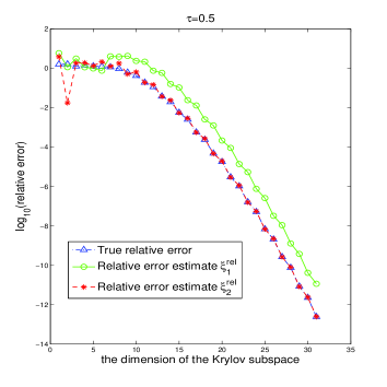
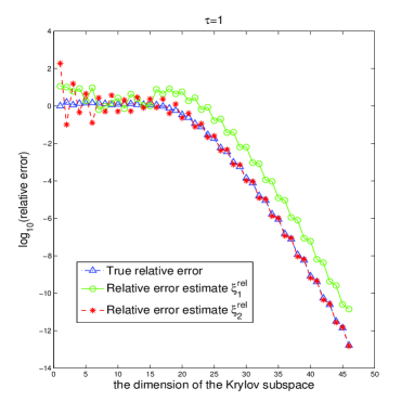
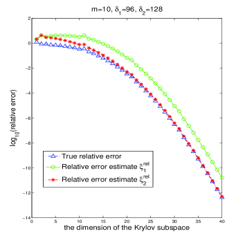
Example 1. We justify the effectiveness of $\xi_{1}^{rel}$ and $\xi_{2}^{rel}$ for $f(A)=e^{-\tau A}$. Consider the diagonal matrix $A$ of size $N=1001$ taken from [18] with equidistantly spaced eigenvalues in the interval $[0,\,40]$. The $N$-dimensional vector $v$ is generated randomly in a uniform distribution with $\left\|v\right\|=1$. For this $A$ and $\tau=0.1,\ 0.5,1$, we have $\lambda_{\min}(A)=0$ and $\gamma_{1}=e^{4},\ e^{20},\ e^{40}$, which are approximately $54.6,\ 4.9\times 10^{8},\ 2.4\times 10^{17}$, respectively. We see $\gamma_{1}$ varies drastically with increasing $\tau$. The corresponding three $\gamma_{3}=\tau\gamma_{1}\|(A-z_{0}I)v_{m+1}\|$ are the same order as $\tau\gamma_{1}\|A\|$ and change in a similar way.

Figure 1: Example 1: The relative error estimates and the true relative error for $e^{-\tau A}v$ for $A$ symmetric with $N=1001$

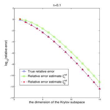
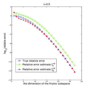
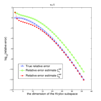
Figure 1 depicts the curves of the two relative error estimates $\xi_{1}^{rel}$, $\xi_{2}^{rel}$ and the true relative error (5.4) for the Lanczos approximations to $e^{-\tau A}v$ with three parameters $\tau=0.1,\,0.5$ and $1$. It is seen that both estimates $\xi_{1}^{rel}$ and $\xi_{2}^{rel}$ are accurate, and particularly $\xi_{2}^{rel}$ is indistinguishable from the true relative error as $m$ increases and is sharper than $\xi_{1}^{rel}$ by roughly one order. Remarkably, it is observed from the figure that the effectiveness of $\xi_{1}^{rel}$ and $\xi_{2}^{rel}$ is little affected by greatly varying $\gamma_{1}$ and $\gamma_{3}$, which themselves critically depend on the spectrum of $A$ and $\tau$. This demonstrates that $\gamma_{1}$ and $\gamma_{3}$ are too conservative, they behave like $O(1)$ in practice and our estimates are accurate and mimic the true error norms very well. However, as a byproduct, we find that the smaller $\tau$ is, the faster the Lanczos approximations converge. So the convergence itself is affected by the size of $\tau$ considerably.

5.2 The case that $A$ is non-Hermitian

Unlike the Hermitian case, for $A$ non-Hermitian, Theorems 4.1 and 4.3 do not give explicit relationships between the error norm and $\xi_{1}$, $\xi_{2}$. So it is not obvious how to use $\xi_{1}$ and $\xi_{2}$ to estimate the true error norm. However, if we lower our standard a little bit, it is instructive to make use of these two theorems to justify the effectiveness of $\xi_{1}^{rel}$ and $\xi_{2}^{rel}$ for estimating the relative error of the Arnoldi approximations to $e^{-\tau A}v$, as shown below.

Define two functions $g_{1}(t)=e_{m}^{T}e^{-tH_{m}}e_{1}$ and $g_{2}(t)=e_{m}^{T}\phi_{1}(-tH_{m})e_{1}$. By continuity, there exist two positive constants $c_{1},\ c_{2}\geq 1$ such that

$$\max_{0\leq t\leq\tau}\left|g_{1}(t)\right|=c_{1}|e_{m}^{T}e^{-\tau H_{m}}e_{1}|\ \text{and}\ \max_{0\leq t\leq\tau}\left|g_{2}(t)\right|=c_{2}|e_{m}^{T}\phi_{1}(-\tau H_{m})e_{1}|.$$

From the above, (4.1) and (4.3), we have

$$\left\|E_{m}(e^{z},\tau)\right\|\leq c_{1}\tau\frac{e^{\tau\mu_{2}}-1}{\tau\mu_{2}}\xi_{1}\ \text{and}\ \left\|E_{m}(e^{z},\tau)\right\|\leq c_{2}\tau(1+\gamma_{2})\xi_{2},$$

where $\mu_{2}=\mu_{2}[-A]$ and $\gamma_{2}$ is defined as (4.18). Provided that $c_{1}$ or $c_{2}$ is not large, $\xi_{1}$ or $\xi_{2}$ is expected to estimate the true error norm reliably. However, we should be aware that $\xi_{1}$ or $\xi_{2}$ may underestimate the true error norms considerably in the non-Hermitian case when $c_{1}$ or $c_{2}$ is large.

The following example illustrates the behavior of $\xi_{1}^{rel}$ and $\xi_{2}^{rel}$ for $A$ non-Hermitian and their effectiveness of estimating the relative error in (5.4).

Example 2. This example is taken from [12, Example 5.3], and considers the initial boundary value problem

$$\dot{u}-\Delta u+\delta_{1}u_{x_{1}}+\delta_{2}u_{x_{2}}=0 \text{on}\ (0,\,1)^{3}\times(0,\,T),$$

$$u(x,t)=0 \text{on}\ \partial(0,\,1)^{3}\ \text{for all}\ t\in[0,\,T],$$

$$u(x,0)=u_{0}(x), x\in(0,\,1)^{3}.$$

Discretizing the Laplacian by the seven-point stencil and the first-order derivatives by central differences on a uniform meshgrid with meshsize $h=1/(n+1)$ leads to an ordinary initial value problem

$$\dot{u}(t) = -Au(t),\ t\in(0,\,T),$$

$$u(0) = u_{0}.$$

The nonsymmetric matrix $A$ of order $N=n^{3}$ can be represented as the Kronecker product form

$$A=-\frac{1}{h^{2}}[I_{n}\otimes(I_{n}\otimes C_{1})+(B\otimes I_{n}+I_{n}\otimes C_{2})\otimes I_{n}].$$

Here $I_{n}$ is the identity matrix of order $n$ and

$$B={\rm tridiag}(1,-2,1),\ C_{j}={\rm tridiag}(1+\zeta_{j},-2,1-\zeta_{j}),\ j=1,2,$$

where $\zeta_{j}=\delta_{j}h/2$. This is a popular test problem as the eigenvalues of $A$ are explicitly known. Furthermore, if $\mid\zeta_{j}\mid>1$ for at least one $j$, the eigenvalues of $A$ are complex and lie in the right plane. For the spectral properties of $A$, refer to [12, 23].

As in [12], we choose $h=1/15,\ \delta_{1}=96,\ \delta_{2}=128$, which leads to $N=2744$ and $\zeta_{1}=3.2$, $\zeta_{2}\approx 4.27$, and approximate $e^{-\tau A}v$ where $\tau=h^{2}$ and $v=[1,1,\ldots,1]^{T}$. We compare relative error estimates $\xi_{1}^{rel}$ and $\xi_{2}^{rel}$ defined by (5.5) with the true relative error defined by (5.4). The convergence curves of these three quantities are depicted in Figure 2. Similar to the case where $A$ is Hermitian, we observe that $\xi_{1}^{rel}$ and $\xi_{2}^{rel}$ both have excellent behavior, and they mimic the true relative error very well. Particularly, the $\xi_{2}^{rel}$ are almost identical to the true relative errors, and are more accurate than the $\xi_{1}^{rel}$ by about one order.

Figure 2: Example 2: The relative error estimates and the true relative error for $e^{-\tau A}v$ for $A$ nonsymmetric with order $N=2744$.

5.3 Applications to other matrix functions

Theorem 3.1 has indicated that the error expansion works for all sufficiently smooth functions, so it applies to $\sin(z)$ and $\cos(z)$. Furthermore, as analyzed and elaborated in Remark 3.2, just as for $e^{-\tau A}v$, the first term of (3.6) is generally a good error estimate of the Arnoldi approximation to these matrix functions acting on a vector. We now confirm the effectiveness of $\xi_{2}^{rel}$ for $\sin(A)v$ and $\cos(A)v$. We also test the behavior of $\xi_{1}^{rel}$ for these two functions.

Example 3. We consider the Arnoldi approximation to $\cos(-\tau A)v$. Here we choose the matrix $A$ and the vector $v$ as in Example 1 for the symmetric case and as in Example 2 for the nonsymmetric case, respectively.

Figure 3: Example 3: The relative error estimates and the true relative error for $\cos(-\tau A)v$ for $A$ symmetric with $N=1001$

Figure 4: Example 3: The relative error estimates and the true relative error for $\cos(-\tau A)v$ for $A$ is nonsymmetric with $N=2744$

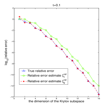
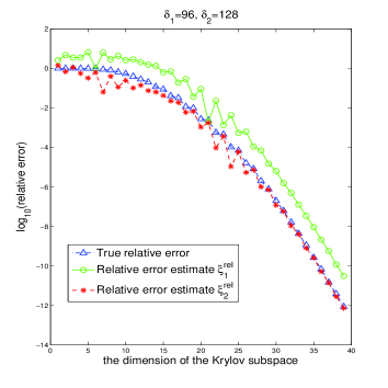
Figures 3–4 illustrate the behavior of $\xi_{1}^{rel}$ and $\xi_{2}^{rel}$ when computing $\cos(-\tau A)v$ for $A$ symmetric and nonsymmetric, respectively. For $A$ symmetric, the $\xi_{2}^{rel}$ are not accurate and underestimate or overestimate the true relative errors in the first few steps for $\tau=0.5,1$. However, as commented in Section 5.1, this does not cause any problem because, during this stage, the true relative errors also stay around one and the Lanczos approximations have no accuracy. After this stage, $\xi_{1}^{rel}$ and especially $\xi_{2}^{rel}$ soon become smooth and provide accurate estimates for the true relative errors as $m$ increases. In particular, the $\xi_{2}^{rel}$ have little difference with the true relative errors for the given three $\tau$. For the error estimates of the Lanczos approximations to $\sin(-\tau A)v$, we have very similar findings, so we do not report the results on it.

For $\cos(-\tau A)v$ with nonsymmetric, the $\xi_{1}^{rel}$ and especially $\xi_{2}^{rel}$ also exhibit excellent behavior and are quite accurate to estimate the true relative error for each $m$ when the latter starts becoming small. Moreover, the $\xi_{2}^{rel}$ are more accurate than $\xi_{1}^{rel}$ and mimic the true relative errors very well when the Arnoldi approximation starts converging. So we conclude that $\xi_{2}^{rel}$ is very reliable to measure the true relative error of the Arnoldi approximations to other analytic functions. For $\sin(-\tau A)v$, we have observed very similar phenomena.

5.4 Applications to other Krylov-like decompositions

The error expansion in Theorem 3.1 holds for the Krylov-like decomposition, which includes the restarted Krylov subspace method for approximating $f(A)v$ proposed in [12] as a special case. We now confirm the effectiveness of $\xi_{1}^{rel}$ and $\xi_{2}^{rel}$ for the restarted Krylov subspace method for approximating $e^{-\tau A}v$ and $\cos(-\tau A)v$.

Example 4. Consider the restarted Krylov algorithm [12] for approximating $e^{-\tau A}v$ and $\cos(-\tau A)v$ by choosing the matrix $A$ and the vector $v$ as in Example 2. The method is restarted after each $m$ steps until the true relative error in (5.4) drops below $\epsilon=10^{-12}$. We test the algorithm with $m=5,\,10$, respectively.

Figure 5: Example 4: The relative error estimates and the true relative error for $e^{-\tau A}v$

Figure 6: Example 4: The relative error estimates and the true relative error for $\cos(-\tau A)v$

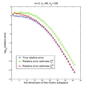
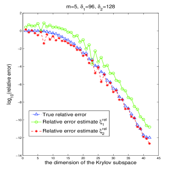
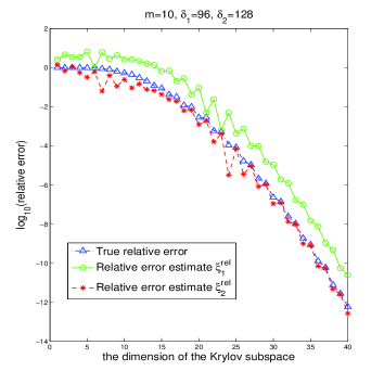
Figures 5–6 illustrate the behavior of $\xi_{1}^{rel}$ and $\xi_{2}^{rel}$ when computing $e^{-\tau A}v$ and $\cos(-\tau A)v$ by the restarted algorithm, where the $x$-axis denotes the sum of dimensions of Krylov subspaces. As in the case that the (non-restarted) Arnoldi approximations in Example 2, we observe that for approximating $e^{-\tau A}v$ by the restarted algorithm, both $\xi_{1}^{rel}$ and $\xi_{2}^{rel}$ exhibit excellent behavior, and the $\xi_{2}^{rel}$ are almost identical to the true relative errors, and are more accurate than the $\xi_{1}^{rel}$ by about one order. For approximating $\cos(-\tau A)v$, similar to Example 3, the $\xi_{1}^{rel}$ and $\xi_{2}^{rel}$ are still quite accurate to estimate the true relative errors when the latter starts becoming small. We have observed the same behavior for approximating $\sin(-\tau A)v$. Particularly, the $\xi_{2}^{rel}$ are considerably better than the $\xi_{1}^{rel}$ and mimic the true relative errors very well when the restarted Arnoldi approximation starts converging. Therefore, we may well claim that, for both non-restarted Arnoldi approximations and the restarted Krylov-like approximations, $\xi_{2}^{rel}$ is very reliable to measure the true relative error of the Krylov-like approximations for $f(z)=e^{z}$ and $\cos(z),\ \sin(z)$.

6 Conclusion

We have generalized the error expansion of the Arnoldi approximation to $e^{A}v$ to the case of Krylov-like approximations for sufficiently smooth functions $f(z)$. We have derived two new a priori upper bounds for the Arnoldi approximation to $e^{-\tau A}v$ and established more compact results for $A$ Hermitian. From them, we have proposed two practical a posteriori error estimates for the Arnoldi and Krylov-like approximations. For the matrix exponential, based on the new error expansion, we have quantitatively proved that the first term of the expansion is a reliable estimate for the whole error, which has been numerically confirmed to be very accurate to estimate the true error. For sufficiently smooth functions $f(z)$, we have shown why the first term of the error expansion can also be a reliable error estimate for the whole error. We have numerically confirmed the effectiveness of them for the cosine and sine matrix functions frequently occurring in applications. It is worthwhile to point out that $\xi_{2}$ is experimentally more accurate than $\xi_{1}$ for the exponential, cosine and sine functions.

We have experimentally found that, for $A$ Hermitian, the reliability of $\xi_{1}^{rel}$ and $\xi_{2}^{rel}$ is not affected by $\gamma_{1}$ and $\gamma_{3}$, respectively, and they are equally accurate to mimic the true relative error for greatly varying $\gamma_{1}$ and $\gamma_{3}$. Therefore, we conjecture that $\gamma_{1}$ and $\gamma_{3}$ can be replaced by some other better forms, at least for $A$ real symmetric semipositive or negative, whose sizes, unlike $e^{\tau(b-a)}$, vary slowly with $\tau$ increasing and the spectrum of $A$ spreading.

Acknowledgements. We thank two referees very much for their very careful reading, valuable comments and constructive suggestions, which enable us to improve the presentation considerably.

References

- [1] M. Abramowitz and I. A. Stegun, Handbook of Mathematical Functions with Formulas, Graphs, and Mathematical Tables, Dover Publications, INC., New York, 1964.
- [2] M. Afanasjew, M. Eiermann, O. G. Ernst, and S. Güttel, A generalization of the steepest descent method for matrix functions, Electron. Trans. Numer. Anal., 28 (2008), pp. 206–222.
- [3] M. Afanasjew, M. Eiermann, O. G. Ernst, and S. Güttel, Implementation of a restarted Krylov subspace method for the evaluation of matrix functions, Linear Algebra Appl., 429 (2008), pp. 229–314.
- [4] C. Beattie, M. Embree, and J. Rossi, Convergence of restarted Krylov subspaces to invariant subspaces, SIAM J. Matrix Anal. Appl., 25 (2004), pp. 1074–1109.
- [5] L. Bergamaschi and M. Vianello, Efficient computation of the exponential operator for large, sparse, symmetric matrices, Numer. Linear Algebra Appl., 7 (2000), pp. 27–45.
- [6] M. A. Botchev, V. Grimm and M. Hochbruck, Residuals, restarting and Richardson iteration for the matrix exponential, SIAM J. Sci. Comput., 35 (2013), pp. 1376–1397.
- [7] K. Dekker and J. G. Verwer, Stability of Runge-Kutta methods for stiff nonlinear differential equations, North Holland, Amsterdam, 1984.
- [8] F. Diele, I. Moret, and S. Ragni, Error estimates for polynomial Krylov approximations to matrix functions, SIAM J. Matrix Anal. Appl., 30 (2008), pp. 1546–1565.
- [9] V. Druskin, On monotonicity of the Lanczos approximation to the matrix exponential, Linear Algebra Appl., 429 (2008), pp. 1679–1683.
- [10] V. L. Druskin and L. A. Knizhnerman, Two polynomial methods of calculating functions of symmetric matrices, Comput. Math. Math. Phys., 29 (1989), pp. 112–121.
- [11] V. L. Druskin and L. A. Knizhnerman, Extended Krylov subspaces: approximation of the matrix square root and related functions, SIAM J. Matrix Anal. Appl., 19 (1998), pp. 775–771.
- [12] M. Eiermann and O. G. Ernst, A restarted Krylov subspace method for the evaluation of matrix functions, SIAM J. Numer. Anal., 44 (2006), pp. 2481–2504.
- [13] M. Eiermann, O. G. Ernst, and S. Güttel, Deflated restarting for matrix functions, SIAM J. Matrix Anal. Appl., 32 (2011), pp. 621–641.
- [14] J. V. Eshof and M. Hochbruck, Preconditioning Lanczos approximations to the matrix exponential, SIAM J. Sci. Comput., 27 (2006), pp. 1438–1457.
- [15] A. Frommer, Monotone convergence of the Lanczos approximations to matrix functions of Hermitian matrices, Electron. Trans. Numer. Anal., 35 (2009), pp. 118–128.
- [16] E. Gallopoulos and Y.Saad, Efficient solution of parabolic equations by Krylov approximation method, SIAM J. Sci. Statist. Comput., 13 (1992), pp. 1236–1264.
- [17] N. J. Higham, Functions of Matrices, SIAM, Philadelphia, PA, 2008.
- [18] M. Hochbruck and C. Lubich, On Krylov subspace approximations to the matrix exponential operator, SIAM J. Numer. Anal., 34 (1997), pp. 1911–1925.
- [19] M. Hochbruck, C. Lubich, and H. Selhofer, Exponential integrators for large systems of differential equations, SIAM J. Sci. Comput., 19 (1998), pp. 1552–1574.
- [20] R. A. Horn and C. R. Johnson, Topics in Matrix Analysis, Cambridge University Press, Cambridge, 1991.
- [21] M. Ilić, I. W. Turner, and D. P. Simpson, A restarted Lanczos approximation to functions of a symmetric matrix, IMA J. Numer. Anal., 30 (2010), pp. 1044–1061.
- [22] L. Lopez and V. Simoncini, Analysis of projection methods for rational function approximation to the matrix exponential, SIAM J. Numer. Anal., 44 (2006), pp. 613–635.
- [23] I. Moret and P. Novati, An interpolatory approximation of the matrix exponential based on Faber polynomials, Comput. Appl. Math., 131 (2001), pp. 361–380.
- [24] I. Moret and P. Novati, Interpolating functions of matrices on zeros of quasi-kernel polynomials, Numer. Linear Algebra Appl., 12 (2005), pp. 337–353.
- [25] R. B. Morgan, A restarted GMRES method augmented with eigenvectors, SIAM J. Matrix Anal. Appl., 16 (1995), pp. 1154–1171.
- [26] R. B. Morgan, GMRES with deflated restarting, SIAM J. Sci. Comput., 24 (2002), pp. 20–37.
- [27] P. Novati, A method based on Fejr points for the computation of functions of nonsymmetric matrices, Appl. Numer. Math., 44 (2003), pp. 201–224.
- [28] B. N. Parlett, Global convergence of the basic QR algorithm on Hessenberg matrices, Math. Comp., 22 (1968), pp. 803–817.
- [29] B. Philippe and R. B. Sidje, Transient solutions of Markov processes by Krylov subspaces, INRIA TR No. 1989 (1993), http://hal.archives-ouvertes.fr/docs/00/07/46/83/PDF/RR-1989.pdf
- [30] Y. Saad, Analysis of some Krylov subspace approximations to the matrix exponential operator, SIAM J. Numer. Anal., 29 (1992), pp. 209–228.
- [31] Y. Saad, Iterative Method for Sparse Linear Systems, Second Edition, SIAM, Philadelphia, PA, 2003.
- [32] R. B. Sidje, Expokit: A software package for computing matrix exponentials, ACM Trans. Math. Software, 24 (1998), pp. 130–156.
- [33] D. C. Sorensen, Implicit application of polynomial filters in a -step Arnoldi method, SIAM J. Matrix Anal. Appl., 13 (1992), pp. 357–385.
- [34] D. E. Stewart and T. S. Leyk, Error estimates for Krylov subspace approximations of matrix exponentials, Comput. Appl. Math., 72 (1996), pp. 359–369.
- [35] G. W. Stewart, A Krylov-Schur algorithm for large eigenproblems, SIAM J. Matrix Anal. Appl., 23 (2001), pp. 601–614.
- [36] T. Ström, On logarithmic norms, SIAM J. Numer. Anal., 12 (1975), pp. 741–753.
- [37] H. Tal-Ezer, Spectral methods in time for parabolic problems, SIAM J. Numer. Anal., 26 (1989), pp. 1–11.
- [38] H. Tal-Ezer, On restart and error estimation for Krylov approximation of , SIAM J. Sci. Comput., 29 (2007), pp. 2426–2441.
- [39] J. van den Eshof, T. L. A. Frommer, and H. A. van der Vorst, Numerical methods for the QCD overlap operator. I. Sign-function and error bounds, Comput. Phys. Comm., 146 (2002), pp. 203–224.
- [40] Q. Ye, Error bounds for the Lanczos methods for approximating matrix exponentials, SIAM J. Numer. Anal., 51 (2013), pp. 68–87.
- [41] P. Zhang, Iterative methods for computing eigenvalues and exponentials of large matrices, Ph.D. thesis, Department of Mathematics, University of Kentucky, Lexington, Kentucky, 2009.