CRPS M-estimation for max-stable models

Abstract

Max-stable random fields provide canonical models for the dependence of multivariate extremes. Inference with such models has been challenging due to the lack of tractable likelihoods. In contrast, the finite dimensional cumulative distribution functions (CDFs) are often readily available and natural to work with. Motivated by this fact, in this work we develop an M-estimation framework for max-stable models based on the continuous ranked probability score (CRPS) of multivariate CDFs. We start by establishing conditions for the consistency and asymptotic normality of the CRPS-based estimators in a general context. We then implement them in the max-stable setting and provide readily computable expressions for their asymptotic covariance matrices. The resulting point and asymptotic confidence interval estimates are illustrated over popular simulated models. They enjoy accurate coverages and offer an alternative to composite likelihood based methods.

1 Introduction

Max-stable processes are a canonical class of statistical models for multivariate extremes. They appear in a variety of applications ranging from insurance and finance (Embrechts et al, 1997; Finkenstädt and Rootzén, 2004) to spatial extremes such as precipitation (Davison and Blanchet, 2011; Davison et al, 2012) and extreme temperature. Max-stable processes are exactly the class of non-degenerate stochastic processes that arise from limits of independent component-wise maxima. This fact provides a theoretical justification for their use as models of multivariate extremes. However, many useful max-stable models suffer from intractable likelihoods, thus prohibiting standard maximum likelihood and Bayesian inference. This has motivated development of maximum composite likelihood estimators (MCLE) for max-stable models (Padoan et al, 2010) as well as certain approximate Bayesian approaches (Reich and Shaby, 2012; Erhardt and Smith, 2011).

In contrast to their likelihoods, the cumulative distribution functions (CDFs) for many max-stable models are available in closed form, or they are tractable enough to approximate within arbitrary precision. This motivates statistical inference based on the minimum distance method (Wolfowitz, 1957; Parr and Schucany, 1980). In this paper, we propose an M-estimator for parametric max-stable models based on minimizing distances of the type

$$\int_{\mathbb{R}^{d}}\left(F_{\theta}\left(x\right)-F_{n}\left(x\right)\right)^{2}\mu\left(dx\right).$$ (1)

where $F_{\theta}$ is a $d$-dimensional CDF of a parametric model, $F_{n}$ is a corresponding empirical CDF and $\mu$ is a tuning measure that emphasizes various regions of the sample space $\mathbb{R}^{d}.$ Using elementary manipulations it can be shown that minimizing distances of the type (1) is equivalent to minimizing the continuous ranked probability score (CRPS).

Definition 1.

(CRPS M-estimator) Let $\mu$ be a measure that can be tuned to emphasize regions of a sample space $\mathbb{R}^{d}$. Define the CRPS functional

$$\mathcal{E}_{\theta}\left(x\right)=\int_{\mathbb{R}^{d}}\left(F_{\theta}\left(y\right)-\mathbf{1}_{\left\{x\leq y\right\}}\right)^{2}\mu\left(dy\right)$$ (2)

Then for independent random vectors $\left\{X^{\left(i\right)}\right\}_{i=1}^{n}$ with common distribution function $F_{\theta_{0}}$ we define the following CRPS M-estimator for $\theta_{0}$.

$$\hat{\theta}_{n}=\underset{\theta\in\Theta}{\text{argmin}}\sum_{i=1}^{n}\mathcal{E}_{\theta}\left(X^{\left(i\right)}\right).$$ (3)

For simplicity, we shall assume throughout that the parameter space $\Theta$ is a compact subset of $\mathbb{R}^{p}$, for some integer $p$.

The remainder of this paper is organized as follows. In Section 2 we review some essential multivariate extreme value theory and provide definitions and constructions of max-stable models. In Section 3 we establish regularity conditions for consistency and asymptotic normality of the CRPS M-estimator and provide general formulae for calculating its asymptotic covariance matrix. In Section 4 we specialize these calculations to the max-stable setting. In Section 5 we conduct a simulation study to evaluate the proposed estimator for popular max-stable models.

2 Extreme values and max-stability

Let $Y^{(i)}=\{Y^{(i)}_{t}\}_{t\in T},\ i=1,2,\cdots$ be independent and identically distributed measurements of certain environmental or physical phenomena. For example, the $Y_{t}^{(i)}$s may model wave-height, temperature, precipitation, or pollutant concentration levels at a site $t$ in a spatial region $T\subset{\mathbb{R}}^{2}$. If one is interested in extremes, it is natural to consider the asymptotic behavior of the point-wise maxima. Suppose that, for some $a_{n}(t)>0$ and $b_{n}(t)\in{\mathbb{R}}$, we have

$${\Big{\{}}\frac{1}{a_{n}(t)}\max_{i=1,\cdots,n}Y_{t}^{(i)}-b_{n}(t){\Big{\}}}_{t\in T}\stackrel{{\scriptstyle d}}{{\longrightarrow}}\{X_{t}\}_{t\in T},\ \mbox{ as }n\to\infty,$$ (4)

for some non-trivial limit process $X$, where $\stackrel{{\scriptstyle d}}{{\to}}$ denotes convergence of the finite-dimensional distributions. The class of extreme value processes $X=\{X_{t}\}_{t\in T}$ arising in the limit describe the statistical dependence of ‘worst case scenaria’ and are therefore natural models of multivariate extremes. The limit $X$ in (4) is necessarily a max-stable process in the sense that for all $n$, there exist $c_{n}(t)>0$ and $d_{n}(t)\in{\mathbb{R}}$, such that

$${\Big{\{}}\frac{1}{c_{n}(t)}\max_{i=1,\cdots,n}X_{t}^{(i)}-d_{n}(t){\Big{\}}}_{t\in T}\stackrel{{\scriptstyle d}}{{=}}\{X_{t}\}_{t\in T},$$

where $\{X^{(i)}_{t}\}_{t\in T}$ are independent copies of $X$ and where $\stackrel{{\scriptstyle d}}{{=}}$ means equality of finite-dimensional distributions (Ch.5 of Resnick, 1987). Due to the classic results of Fisher-Tippett and Gnedenko, the marginals of $X$ are necessarily extreme value distributions (Fréchet, reversed Weibul or Gumbel). They can be described in a unified way through the generalized extreme value distribution (GEV):

$$G_{\xi,\mu,\sigma}(x):=\exp{\Big{\{}}-(1+\xi(x-\mu)/\sigma)_{+}^{-1/\xi}{\Big{\}}},\ \sigma>0,$$ (5)

where $x_{+}=\max\{x,0\}$, and where $\mu,\sigma$ and $\xi$ are known as the location, scale and shape parameters. The cases $\xi>0,\xi<0,$ and $\xi\to 0$ correspond to Fréchet, reverse Weibull, and Gumbel, respectively (see, e.g. Ch.3 and 6.3 in Embrechts et al, 1997 for more details).

The dependence structure of the limit extreme value process $X$ rather than its marginals is of utmost interest in practice. Arguably, the type of the marginals is unrelated to the dependence structure of $X$ and as it is customarily done, we shall assume that the limit process $X$ has been transformed to standard $1$-Fréchet marginals. That is,

$${\mathbb{P}}(X_{t}\leq x)=G_{1,1,\sigma_{t}}(x)=e^{-\sigma_{t}/x},\ x>0,$$ (6)

for some scale $\sigma_{t}>0$ (Ch.5 of Resnick, 1987).

2.1 Representations of max-stable processes

Let $X=\{X_{t}\}_{t\in T}$ be a max-stable process with $1$-Fréchet marginals as in (6). Then, its finite-dimensional distributions are multivariate max-stable random vectors and they have the following representation:

$${\mathbb{P}}(X_{t_{i}}\leq x_{i},\ i=1,\cdots,d)=\exp{\Big{\{}}-\int_{{\mathbb{S}}_{+}^{d-1}}{\Big{(}}\max_{i=1,\cdots,d}w_{i}/x_{i}{\Big{)}}H(dw){\Big{\}}},$$ (7)

where $x_{i}>0,\ t_{i}\in T,\ i=1,\cdots,d$ and where $H=H_{t_{1},\cdots,t_{d}}$ is a finite measure on the positive unit sphere

$${\mathbb{S}}_{+}^{d-1}=\{w=(w_{i})_{i=1}^{d}\,:\,w_{i}\geq 0,\ \sum_{i=1}^{d}w_{i}=1\}$$

known as the spectral measure of the max-stable random vector $(X_{t_{i}})_{i=1}^{d}$ (see e.g. Proposition 5.11 in Resnick, 1987). The integral in the expression (7) is referred to as the tail dependence function of the max-stable law. We shall often use the notation:

$$V(x)\equiv V_{t_{1},\cdots,t_{d}}(x):=-\log{\mathbb{P}}(X_{t_{i}}\leq x_{i},\ i=1,\cdots,d),$$

where $x=(x_{i})_{i=1}^{d}\in{\mathbb{R}}_{+}^{d}$, for the tail dependence function of the max-stable random vector $(X_{t_{i}})_{i=1}^{d}$.

It readily follows from (7) that for all $a_{i}\geq 0,i=1,\cdots,d$, the max-linear combination

$$\xi:=\max_{i=1,\cdots,d}a_{i}X_{t_{i}}$$

is $1$-Fréchet random variable with scale $\sigma_{\xi}=\int_{{\mathbb{S}}_{+}^{d-1}}(\max_{i=1,\cdots,d}a_{i}w_{i})H(dw)$. Conversely, a random vector $(X_{t_{i}})_{i=1}^{d}$ with the property that all its non-negative max-linear combinations are $1$-Fréchet is necessarily multivariate max-stable (de Haan, 1978). This invariance to max-linear combinations is an important feature that will be used in our estimation methodology (Section 4, below).

Some max-stable models are readily expressed in terms of their spectral measures while others via tail dependence functions. These representations however are not convenient for computer simulation or in the case of random processes, where one needs a handle on all finite-dimensional distributions. The most common constructive representation of max-stable process models is based on Poisson point processes (de Haan, 1984; Schlather, 2002; Kabluchko et al, 2009). See also Stoev and Taqqu (2005) for an alternative.

Indeed, consider a measure space $(S,\mathcal{S},\nu)$ and let $\Pi:=\{(\epsilon_{i},S_{i})\}_{i\in\mathbb{N}}$ be a Poisson point process on $\mathbb{R}^{+}\times S$ with intensity measure $dxd\nu$.

Proposition 1.

Let $g_{t}\in L^{1}(S,{\cal S},\nu),\ t\in T$ be a collection of non-negative integrable functions and let

$$X_{t}:=\int_{S}^{\vee}g_{t}d\Pi\equiv\max_{i\in\mathbb{N}}\epsilon_{i}^{-1}g_{t}(S_{i}),\ \ (t\in T).$$ (8)

Then, the process $X=\{X_{t}\}_{t\in T}$ is max-stable with $1$-Fréchet marginals and finite-dimensional distributions:

$${\mathbb{P}}(X_{t_{i}}\leq x_{i},\ i=1,\cdots,d)=\exp{\Big{\{}}-\int_{S}{\Big{(}}\max_{i=1,\cdots,d}g_{t_{i}}(s)/x_{i}{\Big{)}}\nu(ds){\Big{\}}}.$$ (9)

The proof of this result is sketched in Appendix A.1. Relation (8) is known as the de Haan spectral representation of $X$ and $\{g_{t}\}_{t\in T}\subset L_{+}^{1}(S,{\cal S},\nu)$ as the spectral functions of the process. It can be shown that every separable in probability max-stable process has such a representation (see de Haan, 1984 and Proposition 3.2 in Stoev and Taqqu, 2005).

The max-functional in (8) has the properties of an extremal stochastic integral. Indeed, we have max-linearity:

$$\max_{i=1,\cdots,d}a_{i}X_{t_{i}}=\int_{S}^{\vee}{\Big{(}}\max_{i=1,\cdots,d}a_{i}g_{t_{i}}{\Big{)}}d\Pi,$$

for all $a_{i}\geq 0.$ The above max-linear combination is therefore $1$-Fréchet and has a scale coefficient:

$$\int_{S}{\Big{(}}\max_{i=1,\cdots,d}a_{i}g_{t_{i}}{\Big{)}}d\nu={\Big{\|}}\max_{i=1,\cdots,d}a_{i}g_{t_{i}}{\Big{\|}}_{L^{1}(\nu)}.$$

One can also show that $X_{t}$ and $X_{s}$ are independent, if and only if $g_{t}(u)g_{s}(u)=0$, for $\nu$-almost all $u\in S$. That is, the extremal integrals defining $X_{t}$ and $X_{s}$ are over non-overlapping sets. This shows that for max-stable process models pairwise independence implies independence. Further, $X_{t_{n}}$ converges in probability to $X_{t}$ if and only if $g_{t_{n}}$ converges in $L^{1}(\nu)$ to $g_{t}$, as $n\to\infty$. For more details, see e.g de Haan (1984) and Stoev and Taqqu (2005).

Remark 1.

The expressions (7) and (9) may be related through a change of variables (Proposition 5.11 Resnick, 1987). While the spectral measure $H$ in (7) is unique, a max-stable process has many different spectral function representations. Nevertheless, Relation (8) provides a constructive and intuitive representation of $X$, that can be used to build interpretable models.

2.2 Max-stable models

A great variety of max-stable models can be defined by specifying the measure space $(S,\mathcal{S},\nu)$ and an accompanying family of spectral functions $g_{t}$ or equivalently through a consistent family of spectral measures or tail dependence functions. We review next several popular max-stable models and their basic features.

$\bullet$ (Multivariate logistic) Let $X=(X_{t_{i}})_{i=1}^{d}$ have the CDF

$$F_{X}(x)=e^{-V(x)},\ \ \mbox{ where }V(x)=\sigma\times{\Big{(}}\sum_{i=1}^{d}x_{t_{i}}^{-1/\alpha}{\Big{)}}^{\alpha},$$

for $\sigma>0$ and $\alpha\in[0,1].$ The parameter $\alpha$ controls the degree of dependence, where $\alpha=1$ corresponds to independence ($V(x)=\sigma\sum_{i=1}^{d}x_{i}^{-1}$), while $\alpha=0$ to complete dependence ($V(x)=\sigma\max_{i=1,\cdots,d}x_{i}^{-1}$, interpreted as a limit).

This model is rather simple since the dependence is exchangeable but it provides a useful benchmark for the performance of the CRPS-based estimators since the MLE is easy to obtain in this case (see Table 2 below). The recent works of Fougères et al (2009) and Fougères et al (2013) develop far-reaching generalizations of multivariate logistic laws by exploiting connections to sum-stable distributions.

$\bullet$ (Max-linear or spectrally discrete models) Let $A=(a_{ij})_{d\times k}$ be a matrix with non-negative entries and let $Z_{j},\ j=1,\cdots,k$ be independent standard $1$-Fréchet random variables. Define

$$X_{i}=\max_{j=1,\cdots,k}a_{ij}Z_{j},\ \ i=1,\cdots,d.$$ (10)

The vector $X=(X_{i})_{i=1}^{d}$ is max-stable. It can be shown that the CDF of $X$ has the form (7) were the spectral measure

$$H(dw)=\sum_{j=1}^{k}|a_{\cdot j}|\delta_{\{a_{\cdot j}/|a_{\cdot j}|\}}(dw),$$ (11)

is concentrated on the normalized column-vectors of the matrix $A$, i.e. on $a_{\cdot j}/|a_{\cdot j}|:=(a_{ij}/|a_{\cdot j}|)_{i=1}^{d}$, where $|a_{\cdot j}|=\sum_{i=1}^{d}a_{ij}$, and where $\delta_{a}$ stands for the Dirac measure with unit mass at the point $a\in\mathbb{R}^{d}$.

Conversely, any max-stable random vector with discrete spectral measure $H$ has a max-linear representation as in (10), where the columns of the matrix $A$ may be recovered from (11). We shall also call such models spectrally discrete.

Since any spectral measure $H$ can be approximated arbitrarily well with a discrete one, max-linear models are dense in the class of all max-stable models. As argued in Einmahl et al (2012), max-linear distributions arise naturally in economics and finance, as models of extreme losses. The $Z_{j}$s represent independent shock-factors that lead to various extreme losses in a portfolio $X$ depending on the factor loadings $a_{ij}$.

Max-linear models are particularly well-suited for CRPS-based inference, since their tail dependence function has a simple closed form:

$$V(x)=\sum_{j=1}^{k}\max_{i=1,\cdots,d}a_{ij}/x_{i},\ \ x=(x_{i})_{i=1}^{d}\in{\mathbb{R}}_{+}^{d}.$$ (12)

See Section 5 below for a simple example of CRPS-based inference for max-linear models and Einmahl et al (2012) for an alternative M-estimation methodology.

$\bullet$ (Moving maxima and mixed moving maxima) Let $(S,{\cal S},\nu)\equiv({\mathbb{R}}^{k},{\cal B}_{{\mathbb{R}}^{k}},{\rm Leb})$ and $g_{t}(s):=g(t-s),t,s\in{\mathbb{R}}^{k}$, for some non-negative integrable function $g\geq 0$, $\int_{{\mathbb{R}}^{k}}g(s)ds<\infty$. Then (8) yields the so-called moving maxima random field:

$$X_{t}:=\int^{\vee}_{{\mathbb{R}}^{k}}g(t-s)d\Pi(s)\equiv\max_{i\in{\mathbb{N}}}g(t-S_{i})/\epsilon_{i},\ \ (t\in{\mathbb{R}}^{k}).$$

The choice of the kernel $g$ as a multivariate Normal density in ${\mathbb{R}}^{2}$ yields the well-known Smith storm model, where the $S_{i}$s may be interpreted as storm locations, $g$ is the spatial storm attenuation profile and $1/\epsilon_{i}$ its strength.

More flexible models can be obtained by taking maxima of independent moving maxima, resulting in the so-called mixed moving maxima:

$$X_{t}=\int_{{\mathbb{R}}^{k}\times U}^{\vee}g(t-s,u)d\Pi(s,u)\equiv\max_{i\in{\mathbb{N}}}g(t-S_{i},U_{i})/\epsilon_{i},\ \ (t\in{\mathbb{R}}^{k})$$ (13)

where $\Pi$ is a Poisson point process on $S={\mathbb{R}}^{k}\times U$ with intensity $\nu(ds,du)=dsm(du)$, and where $g\geq 0$ is such that $\int_{{\mathbb{R}}^{k}\times U}g(s,u)dsm(du)<\infty$. Here $m(du)$ is the ‘mixing’ measure, which may be continuous or discrete, and the $U_{i}$s may be viewed as different types of storms.

The mixed moving maxima random fields are stationary, ergodic and, in fact, mixing (Stoev, 2008; Kabluchko and Schlather, 2010). By (9), their tail dependence functions are

$$V(x)=\int_{{\mathbb{R}}^{k}\times U}{\Big{(}}\max_{i=1,\cdots,d}g(t_{i}-s,u)/x_{i}{\Big{)}}dsm(du),\ \ x=(x_{i})_{i=1}^{d}\in{\mathbb{R}}_{+}^{d}.$$

$\bullet$ (Spectrally Gaussian models) By viewing $(S,{\cal S},\nu)$ as a probability space, in the case $\nu(S)=1$, the spectral functions $\{g_{t}\}_{t\in T}$ in (8) become a stochastic process. By picking $g_{t}=h(w_{t})$ to be non-negative transformations of a Gaussian process $w_{t}$ on $(S,{\cal S},\nu)$, one obtains interesting and tractable max-stable models whose dependence structure is governed by the covariance structure of the underlying Gaussian process $\{w_{t}\}_{t\in T}$. The popular Smith, Schlather, and Brown-Resnick random field models are of this type (Smith, 1990; Schlather, 2002; Brown and Resnick, 1977; Stoev, 2008; Kabluchko et al, 2009).

$\circ$ (Schalther models) Let $\{w_{t}\}_{t\in{\mathbb{R}}^{k}}$ be a stationary Gaussian random field with zero mean and let $g_{t}(s):=(w_{t}(s))_{+},\ s\in S$. Then $X_{t}$ in (8) has the following tail dependence function

$$V(x)=\mathbb{E}_{\nu}{\Big{(}}\max_{i=1,\cdots,d}(w_{t_{i}})_{+}/x_{i}{\Big{)}},\ \ x=(x_{i})_{i=1}^{d}\in{\mathbb{R}}_{+}^{d},$$ (14)

where $\mathbb{E}_{\nu}$ denotes integration with respect to the ‘probability’ measure $\nu$.

$\circ$ (Brown-Resnick) Let $w=\{w_{t}\}_{t\in{\mathbb{R}}^{k}}$ be a zero mean Gaussian random field with stationary increments. Set $g_{t}(s):=e^{w_{t}(s)-v_{t}/2}$, where $v_{t}=\mathbb{E}_{\nu}(w_{t}^{2})$ is the ‘variance’ of $w_{t}$. The seminal paper of Brown and Resnick (1977) introduced this model with $w$ – the standard Brownian motion and showed that, surprisingly, the resulting max-stable process $X_{t}$ in (8) is stationary, even though $w$ is not. The cornerstone work of Kabluchko et al (2009) showed that $\{X_{t}\}_{t\in{\mathbb{R}}^{k}}$ is stationary for a centered Gaussian process $w$, with stationary increments . It also obtained important mixed moving maxima representations of $X$ under further conditions on $w$. The tail dependence function of $X$ in this case is

$$V(x)=\mathbb{E}_{\nu}{\Big{(}}\max_{i=1,\cdots,d}e^{w_{t_{i}}-v_{t_{i}}/2}/x_{i}{\Big{)}},\ \ x=(x_{i})_{i=1}^{d}\in{\mathbb{R}}_{+}^{d}.$$ (15)

It can be shown that the Smith model (Smith, 1990) is a special case of a Brown-Resnick model with a degenerate random field $\{w_{t}\}\stackrel{{\scriptstyle d}}{{=}}\{t^{\top}Z\},\ t\in{\mathbb{R}}^{k}$, $k<d$, where $Z$ is a Normal random vector in ${\mathbb{R}}^{k}$. The above models can be deemed spectrally Gaussian since their tail dependence functions (and hence spectral measures) are expectations of functions of Gaussian laws. One can consider other stochastic process models for the underlying spectral functions $g_{t}$ and thus arrive at doubly stochastic max-stable processes. We comment briefly on some general probabilistic properties of these models.

Remark 2.

If $\{g_{t}\}_{t\in{\mathbb{R}}^{k}}$ is a stationary process in $(S,{\cal S},\nu)$, then the max-stable process $X=\{X_{t}\}_{t\in{\mathbb{R}}^{k}}$ is also stationary. It is, however, non-ergodic. In particular, the Schlather models are non-ergodic. This is important in applications, since a single observation of the random field $X$ at an expanding grid, may not yield consistent parameter estimates.

Kabluchko et al (2009) have shown that Brown-Resnick random fields with non-stationary $\{w_{t}\}$ such that $\lim_{|t|\to\infty}(w_{t}-v_{t}/s)=-\infty,$ almost surely, have mixed moving maxima representations as in (13). They are therefore mixing (Stoev, 2008) and consistent statistical inference from a single realization of such max-stable random fields is possible.

Remark 3.

The Poisson point process construction in (8) involves a maximum over an infinite number of terms. As a result, computer simulations of spectrally Gaussian max-stable models necessitates truncation to a finite number. In the case of the Brown-Resnick model, the number of terms required to produce a satisfactory representation is prohibitively large. Accurate simulation of Brown-Resnick processes is an active area of study (Oesting et al, 2011). Consequently, simulation studies for inference under Brown-Resnick models have yet to appear. For this reason the remaining discussion of spectrally Gaussian max-stable models including simulation and application is restricted to the Schlather model.

2.3 Measures of dependence in max-stable models

   

$\bullet$ (Co-variation) For $X_{t}$ as in (8), define

$$[X_{t},X_{s}]:=\int_{S}g_{t}\wedge g_{s}d\nu\equiv\int_{S}g_{t}d\nu+\int_{S}g_{s}d\nu-\int_{S}g_{t}\vee g_{s}d\nu,\ (t,s\in T).$$

Note that $\int_{S}g_{t}d\nu$ and $\int_{S}(g_{t}\vee g_{s})d\nu$ are the scale coefficients of the Fréchet random variables $X_{t}$ and $X_{t}\vee X_{s}$. The co-variation $[X_{t},X_{s}]\geq 0$ is non-negative and equals zero if and only if $X_{t}$ and $X_{s}$ are independent, analagous to covariance for Gaussian processes.

$\bullet$ (Extremal coefficient) A popular summary measure of multivariate dependence in max-stable models is the extremal coefficient. Define

$$\vartheta\left(D\right):=-\log\mathbb{P}\left(X_{t}\leq 1,t\in D\right)\equiv V\left(\mathbf{1}\right).$$

For a process $\left\{X_{t},t\in D\right\}$ with standard 1-Fréchet marginals

$$\max_{t\in D}\frac{1}{x_{t}}\leq V\left(x\right)\leq\sum_{t\in D}\frac{1}{x_{t}}$$

and thus $1\leq\vartheta\left(D\right)\leq d=|D|$, where $\vartheta\left(D\right)=1$ corresponds to complete dependence while $\vartheta\left(D\right)=d$ implies that $X_{t}$’s , $t\in D$ are independent.

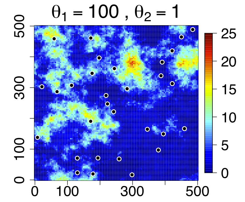
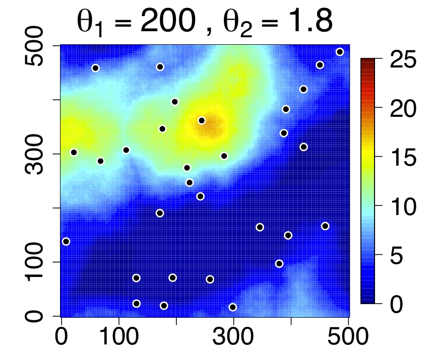
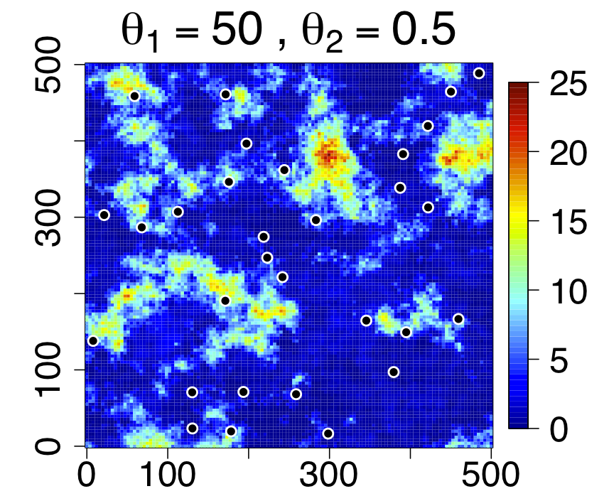
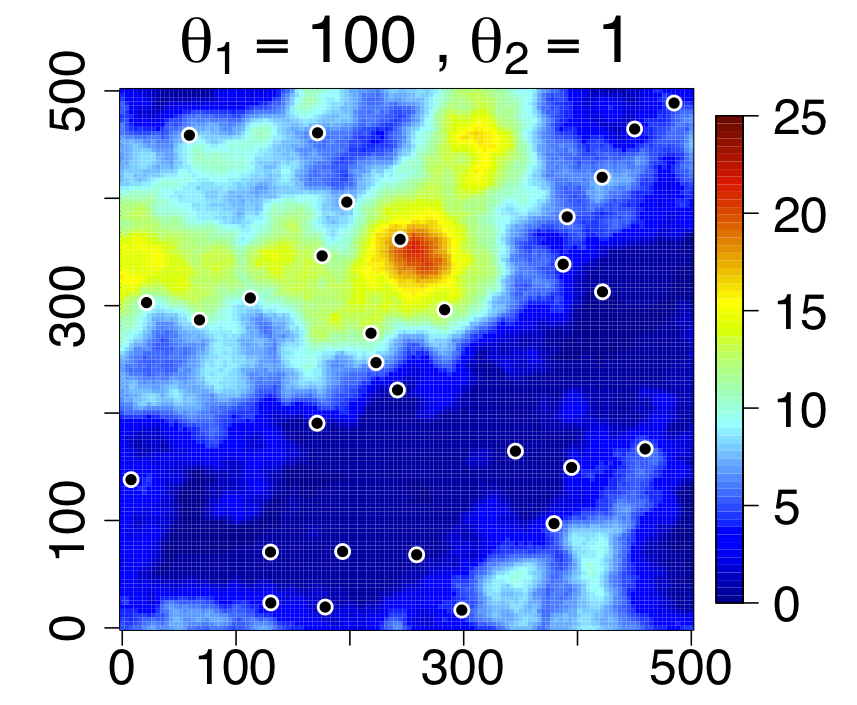
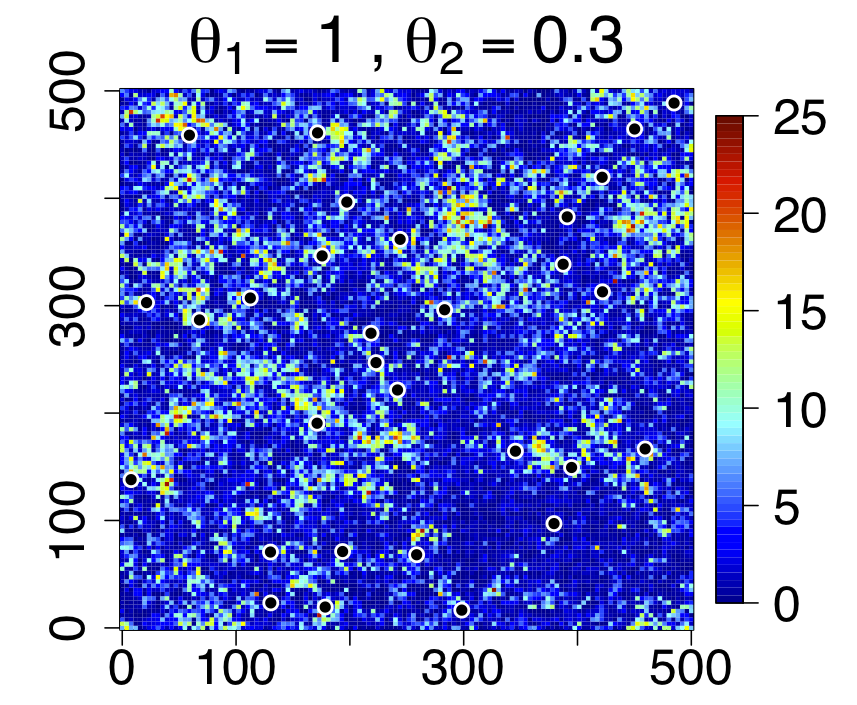
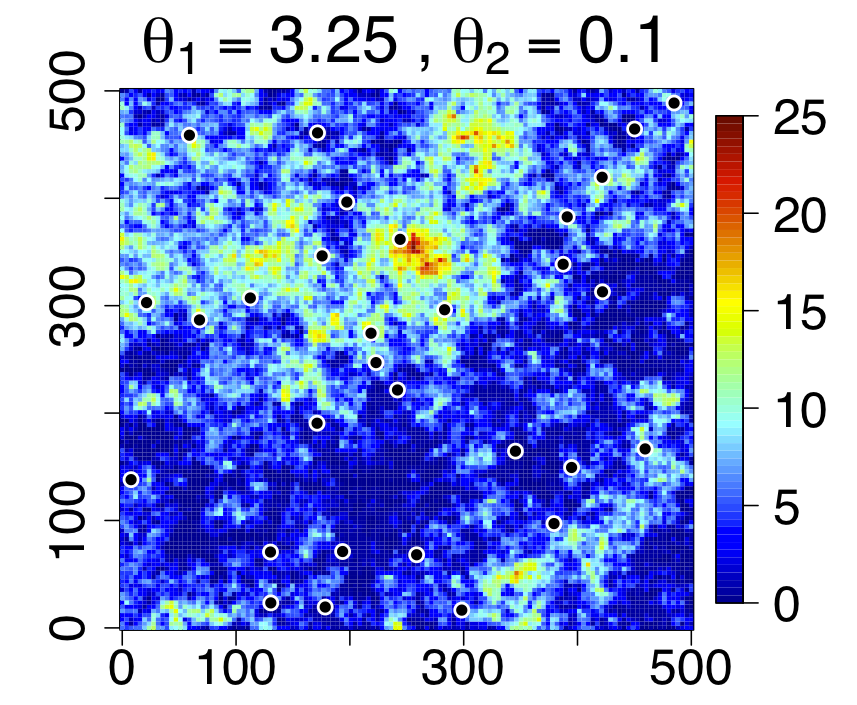
It is well know that for a process with standard $1$-Fréchet marginals, $\vartheta(\{t,t+h\})=2-[X_{t},X_{t+h}]$. In the case of the Schlather model there is an explicit formula for the bivariate extremal coefficient in terms of the correlation function: $\vartheta(\{t,s\})=1+\sqrt{(1-\rho(t,s))/2}$. Figure 1 displays realizations from the Schlather model for the different correlation functions given in Table 1. Note that these examples are all (spectrally) isotropic in the sense that the correlation $\rho\left(t,s\right)$ of the underlying Gaussian process depends only on the distance $h=\left\|t-s\right\|$ between locations $t$ and $s$. This however is not a requirement in general. Figure 1 also provides some visual evidence of how the covariance structure and smoothness of $w$ influence the dependence structure of the resultant max-stable random field $X$. It is possible to parameterize the dependence structure of the max-stable random field using a large variety of covariance functions available for parameterizing Gaussian processes.

Table 1: Correlation functions for Gaussian random fields. For the Matérn covariance function, $K_{\theta_{2}}$ is the modified Bessel function of the second kind.

	$\rho_{\theta}(t,s)$, $h=\|t-s\|$
Stable	$\exp\big{[}-(h/\theta_{1})^{\theta_{2}}\big{]}\quad\theta_{1}>0,\theta_{2}\in(0,2]$
Matérn	$\frac{(\sqrt{2\theta_{2}}h/\theta_{1})^{\theta_{2}}}{\Gamma(\theta_{2})2^{\theta_{2}-1}}{K_{\theta_{2}}\big{(}\sqrt{2\theta_{2}}h/\theta_{1}\big{)}}\quad\theta_{1}>0,\theta_{2}>0$
Cauchy	$(1+(h/{\theta_{1}})^{2})^{-\theta_{2}}\quad\theta_{1}>0,\theta_{2}>0$

Figure 1: Schlather max-stable model realizations using correlation functions of Table 1 under varying parameter settings. Top: Stable correlation function. Middle: Matérn correlation function. Bottom: Cauchy correlation function. Realizations were generated using the R package SpatialExtremes (Ribatet, 2011). The circles indicate locations of “observation staions” in the simulation study of Section 5.

3 Consistency and asymptotic normality of CRPS M-estimators

In this section, we establish general conditions for the consistency and asymptotic normality of CRPS-based M-estimators. This is motivated by questions of inference in max-stable models, but may be of independent interest. Section 4 implements and specializes these results to the max-stable setting.

We start with two theorems that are distillations of well know results from the general theory of M-estimators, for example see van der Vaart (1998). Their proofs are given in Appendix A.2.

Theorem 2.

Let $X,X^{\left(1\right)},X^{\left(2\right)},\ldots$ be iid random vectors with cumulative distribution function $F_{\theta_{0}}.$ Let $\hat{\theta}_{n}$ be as in Definition 1 with $\theta_{0}$ an interior point of $\Theta$. Suppose that the following conditions hold:

(i) (identifiability) For all $\theta_{1},\theta_{2}\in\Theta,$

$$\theta_{1}\not=\theta_{2}\Rightarrow F_{\theta_{1}}\not=F_{\theta_{2}}\quad\text{a.e. }\mu$$ (16)

(ii) (integrability) For $B\left(\theta_{0}\right)\subset\Theta,$ an open neighborhood of $\theta_{0}$

$$\int_{\mathbb{R}^{d}}\sup_{\theta\in B\left(\theta_{0}\right)}\left(1-F_{\theta}\left(x\right)\right)\mu\left(dx\right)<\infty.$$ (17)

(iii) (continuity) The function $\theta\mapsto\int_{\mathbb{R}^{d}}(F_{\theta}(x)-F_{\theta_{0}}(x))^{2}\mu(dx)$ is continuous in the compact parameter space $\Theta\subset\mathbb{R}^{p}$.

Then $\hat{\theta}_{n}\xrightarrow{p}\theta_{0},\ \mbox{as}\ n\to\infty.$

Theorem 3.

Assume the conditions and notation of Theorem 2 hold so that in particular, $\hat{\theta}_{n}\xrightarrow{p}\theta_{0}$. Suppose, moreover, that;

• The measurable function $\theta\mapsto\mathcal{E}_{\theta}\left(x\right)$ is differentiable at $\theta_{0}$ (for almost every $x$) with gradient

  $$\dot{\mathcal{E}}_{\theta_{0}}\left(x\right):=\left.\frac{\partial}{\partial\theta}\mathcal{E}_{\theta}\left(x\right)\right|_{\theta=\theta_{0}}.$$

• There exists a measurable function $L\left(x\right)$ with $\mathbb{E}\left(L\left(X\right)\right)^{2}<\infty$, such that for every $\theta_{1}$ and $\theta_{2}$ in $B\left(\theta_{0}\right)$

  $$\left|\mathcal{E}_{\theta_{1}}\left(x\right)-\mathcal{E}_{\theta_{2}}\left(x\right)\right|\leq L\left(x\right)\left\|\theta_{1}-\theta_{2}\right\|.$$ (18)

• The map $\theta\mapsto\mathbb{E}\mathcal{E}_{\theta}\left(X\right)$ admits a second-order Taylor expansion at the point of minimum $\theta_{0}$ with non-singular second derivative matrix

  $$H_{\theta_{0}}:=\left.\frac{\partial^{2}}{\partial\theta\partial\theta^{\top}}\mathbb{E}\mathcal{E}_{\theta}\left(X\right)\right|_{\theta=\theta_{0}}.$$ (19)

Then

$$\sqrt{n}\left(\hat{\theta}_{n}-\theta_{0}\right)\xrightarrow{d}\mathcal{N}\left(0,H_{\theta_{0}}^{-1}J_{\theta_{0}}H_{\theta_{0}}^{-1}\right),\ \ \mbox{as\ n$\to\infty$,}$$ (20)

where

$$J_{\theta_{0}}:=\mathbb{E}\left\{\dot{\mathcal{E}}_{\theta_{0}}\left(X\right)\dot{\mathcal{E}}_{\theta_{0}}\left(X\right)^{\top}\right\}.$$ (21)

The following result provides explicit conditions on the family of CDFs $\left\{F_{\theta},\theta\in\Theta\right\}$ that imply conditions (i)-(iii) of Theorem 3. It also gives concrete expressions for the “bread” and “meat” matrices $H_{\theta_{0}}$ and $J_{\theta_{0}}$ in terms of $F_{\theta}$, which can be used to compute the asymptotic covariances in (20). The proof is given in Appendix A.2.

Proposition 2.

Assume the conditions and notation in Theorem 2. Suppose moreover that:

• $\theta\mapsto F_{\theta}\left(y\right)$ is twice continuously differentiable for all $\theta$ in $B\left(\theta_{0}\right)$ with gradient $\dot{F}_{\theta}\left(y\right):=\partial F_{\theta}\left(y\right)/\partial\theta$ and second derivative matrix $\ddot{F}_{\theta}\left(y\right):=\partial^{2}F_{\theta}\left(y\right)/\partial\theta\partial\theta^{\top}.$

• For all $a\in\mathbb{R}^{p}$ with $\left\|a\right\|>0$

  $$\int_{\mathbb{R}^{d}}\left(a^{\top}\dot{F}_{\theta_{0}}\left(y\right)\right)^{2}\mu\left(dy\right)>0.$$ (22)

• $\int_{\mathbb{R}^{d}}\sup_{\theta\in B\left(\theta_{0}\right)}\left(\|\dot{F}_{\theta}\left(y\right)\|+\|\dot{F}_{\theta}\left(y\right)\|^{2}+\|\ddot{F}_{\theta}\left(y\right)\|\right)\mu\left(dy\right)<\infty$.

Then (i)-(iii) of Theorem 3 are satisfied and therefore (20) holds, where

$$H_{\theta_{0}}:=2\int_{\mathbb{R}^{d}}\dot{F}_{\theta_{0}}\left(y\right)\dot{F}_{\theta_{0}}\left(y\right)^{\top}\mu\left(dy\right)$$ (23)

and

$$J_{\theta_{0}}:=4\int_{\mathbb{R}^{d}}\int_{\mathbb{R}^{d}}\beta_{\theta_{0}}\left(y_{1},y_{2}\right)\dot{F}_{\theta_{0}}\left(y_{1}\right)\dot{F}_{\theta_{0}}\left(y_{1}\right)^{\top}\mu\left(dy_{1}\right)\mu\left(dy_{2}\right)$$ (24)

where $\beta_{\theta_{0}}\left(y_{1},y_{2}\right)=F_{\theta_{0}}\left(y_{1}\wedge y_{2}\right)-F_{\theta_{0}}\left(y_{1}\right)F_{\theta_{0}}\left(y_{2}\right).$

Remark 4.

Practical inference utilizing the CRPS M-estimator is limited to cases where optimization of $\theta\mapsto\mathcal{E}_{\theta}$ is feasible. Likewise, confidence intervals are only obtained when the matrices $H_{\theta_{0}}^{-1},J_{\theta_{0}}$ can be computed. Given the multivariate integration involved, this may require specialized methods for various models. In the max-stable setting this is achieved through judicious specification of the measure $\mu$, discussed in the following section.

Remark 5.

Condition (22) ensures that the “bread” matrix $H_{\theta_{0}}$ in (23) is non-singular. It is rather mild and fails only if the gradient $\dot{F}_{\theta_{0}}\left(y\right)$ lies in a lower dimensional hyper-plane for $\mu$-alomost all $y$. In practice, unless the model is over-parameterized this condition typically holds.

Remark 6.

The expressions (23) and (24) can be used in practice to compute the asymptotic covariance matrix in (20). In Sections 4 and 5 we have implemented numerical and Monte Carlo based methods for calculating $H_{\theta_{0}}$ and $J_{\theta_{0}}$ under the models introduced in Section 2.

4 CRPS M-estimation for max-stable models

Our goal is to implement the general CRPS method of the previous section in the case of multivariate max-stable models described in Section 2. Calculation of the CRPS for such models is aided by a closed form expression of the univariate CRPS for $1$-Fréchet random variates which is given in the following Lemma.

Lemma 1.

Suppose the measure $\mu$ in Definition 1 of the CRPS is specified as $\mu\left(dr\right)=r^{-1/2}dr$ for $r\in\mathbb{R}_{+}.$ Then the univariate CRPS with respect to the $1$-Fréchet distribution function $e^{-v/r}$ has the following closed form

$$\mathfrak{F}\left(m,v\right):=\int_{0}^{\infty}\left(e^{-v/r}-\mathbf{1}_{\left\{m\leq r\right\}}\right)^{2}r^{-1/2}dr\\ =4\left[\sqrt{m}\left(e^{-v/m}-\frac{1}{2}\right)+\sqrt{v}\left(\gamma_{\frac{1}{2}}\left(v/m\right)-\sqrt{\frac{\pi}{2}}\right)\right],$$ (25)

where $\gamma_{\alpha}\left(z\right)=\int_{0}^{z}t^{\alpha-1}e^{-t}dt$ is the incomplete gamma function.

See Appendix A.3 for a proof. We introduce the notation $\mathfrak{F}$ to distinguish the univariate Fréchet CRPS from the multivariate case. The functional $\mathfrak{F}$ is the basis for many of the calculations that follow.

Now recall that the CDF of a $1$-Fréchet max-stable random vector $X=\left(X_{i}\right)_{i=1,\ldots,d}$ is characterized by the tail function $V\left(x\right)$ as follows

$$F_{X}\left(x\right)=\mathbb{P}\left(X_{i}\leq x_{i},i=1,\ldots,d\right)=e^{-V\left(x\right)},$$ (26)

where $V$ exhibits the homogeneity property $V\left(rx\right)=V\left(x\right)/r$ for all $r>0,x\in(0,\infty]^{d}.$ This means that for any $u=\left(u_{i}\right)_{i=1,\ldots,d}\in\mathbb{R}_{+}^{d}$, the max-linear combination

$$M_{u}:=\max_{i=1,\ldots,d}\frac{X_{i}}{u_{i}}$$ (27)

is a $1$-Fréchet variable with scale $V\left(u\right)$. Indeed,

$$\mathbb{P}\left(M_{u}\leq r\right)=\mathbb{P}\left(X_{i}\leq ru_{i},i=1,\ldots,d\right)=e^{-V\left(ru\right)}=e^{-V\left(u\right)/r}.$$

This max-linearity invariance property motivates a particular choice of the measure $\mu$ that appears in Definition 1 for the multivariate CRPS. Let

$$\mu\left(dy\right)\equiv\mu\left(dr,du\right):=r^{-1/2}dr\sum_{w\in\mathcal{U}}\delta_{w}\left(du\right),$$ (28)

where $u=y/\left|y\right|,r=\left|y\right|=\sum_{i=1}^{d}y_{i}\text{ and }\mathcal{U}\subset\mathbb{R}_{+}^{d}.$ With this choice of $\mu$ we have the following closed form expression for the multivariate CRPS in terms of the max-linear combinations $\left\{M_{u}\right\}_{u\in\mathcal{U}}.$

Proposition 3.

With $\mu$ as in (28), for the CRPS in (2), we have

$$\mathcal{E}_{\theta}\left(X\right) =\int_{[0,\infty)^{d}}\left[e^{-V_{\theta}\left(y\right)}-\mathbf{1}_{\left\{X\leq y\right\}}\right]^{2}\mu\left(dy\right)$$

$$=\sum_{u\in\mathcal{U}}\mathfrak{F}\left(M_{u},V_{\theta}\left(u\right)\right)$$ (29)

with $\mathfrak{F}$ as in Lemma 1.

Proof.

Using the substitution $u=y/\left|y\right|$ and $r=\left|y\right|$, specifying the measure $\mu$ as in (28) results in

$$\mathcal{E}_{\theta}\left(X\right) =\int_{[0,\infty)^{d}}\left[e^{-V_{\theta}\left(y\right)}-\mathbf{1}_{\left\{X\leq y\right\}}\right]^{2}\mu\left(dy\right)$$

$$=\sum_{u\in\mathcal{U}}\int_{0}^{\infty}\left[e^{-V_{\theta}\left(ru\right)}-\mathbf{1}_{\left\{X\leq ru\right\}}\right]r^{-1/2}dr.$$

Observe that $\{X\leq ru\}=\left\{X_{i}\leq ru_{i},i=1,\ldots,d\right\}$ is equivalent to $\left\{M_{u}\leq r\right\}$, where $M_{u}$ is as in (27). Therefore, using the homogeneity property $V_{\theta}\left(ru\right)=V_{\theta}\left(u\right)/r$, we obtain

$$\int_{0}^{\infty}\left[e^{-V_{\theta}\left(ur\right)}-\mathbf{1}_{\left\{X\leq ru\right\}}\right]r^{-1/2}dr=\int_{0}^{\infty}\left[e^{-V_{\theta}\left(u\right)/r}-\mathbf{1}_{\left\{M_{u}\leq r\right\}}\right]r^{-1/2}dr.$$

Lemma 1 applied to the last integral yields (29). ∎

In practice, given a set of independent observations $X^{\left(1\right)},X^{\left(2\right)},\ldots,X^{\left(n\right)}$ from the model $F_{\theta_{0}}\left(x\right)=\exp\left(-V_{\theta_{0}}\left(x\right)\right)$ we obtain the CRPS-based estimator of $\theta_{0}$ as follows

CRPS estimation procedure

1. Construct the set $\mathcal{U}\subset\mathbb{R}_{+}^{d}$. The distribution of $\mathcal{U}$ can be determined heuristically. In general, finite uniform random samples from the simplex $\Delta^{d-1}:=\left\{u\in\left(0,1\right)^{d},\left|u\right|=1\right\}$ work well.

2. Construct the max-linear combinations $M_{u}^{\left(i\right)}=\max_{j=1,\ldots,d}X_{j}^{\left(i\right)}/u_{j}$, for all $i=1,\ldots,n$ and $u\in\mathcal{U}$.

3. Using numerical optimization, compute:

   $$\hat{\theta}_{n}=\underset{\theta\in\Theta}{\arg\min}\sum_{i=1}^{n}\sum_{u\in\mathcal{U}}\mathfrak{F}\left(M_{u}^{\left(i\right)},V_{\theta}\left(u\right)\right).$$

In Section 5, we illustrate this methodology over several concrete examples. The explicit construction of the set $\mathcal{U}$ is given in each example and the computation of the tail dependence function $V_{\theta}$ when it is not available in closed form is discussed.

The following result provides readily computable expressions for the “bread” and “meat” matrices appearing in the asymptotic covariance of the CRPS estimators.

Corollary 1.

Using the same specification of the measure $\mu$ as in (28)

$$H_{\theta_{0}}=\frac{\sqrt{\pi}}{2}\sum_{u\in\mathcal{U}}\left(2V_{\theta_{0}}\left(u\right)\right)^{-3/2}\dot{V}_{\theta_{0}}\left(u\right)\left(\dot{V}_{\theta_{0}}\left(u\right)\right)^{\top}$$ (30)

and

$$J_{\theta_{0}}=\sum_{u,w\in\mathcal{U}}c_{\theta_{0}}\left(u,w\right)\frac{\dot{V}_{\theta_{0}}\left(u\right)\left(\dot{V}_{\theta_{0}}\left(w\right)\right)^{\top}}{\sqrt{V_{\theta_{0}}\left(u\right)V_{\theta_{0}}\left(w\right)}}$$ (31)

where

$$c_{\theta_{0}}\left(u,w\right)=\mathrm{Cov}\left\{\gamma_{\frac{1}{2}}\left(V_{\theta_{0}}\left(u\right)/M_{u}\right),\gamma_{\frac{1}{2}}\left(V_{\theta_{0}}\left(w\right)/M_{w}\right)\right\}.$$

Remark 7.

$M_{u}$ and $M_{w}$ are dependent since in view of (27) they are defined as max-linear combinations of the vector $X$. The coefficient $c_{\theta_{0}}\left(u,w\right)$ can be conveniently computed using Monte Carlo methods by simulating a large number of independent copies of $X$ under the $F_{\theta_{0}}$ model. In practice the resulting asymptotic covariance matrix estimates yield confidence intervals with close to nominal coverage (see Tables 2 and 4).

5 Simulation

In this section we conduct simulation studies for CRPS M-estimation under 3 different max-stable models. The first example provides a comparison of CRPS M-estimation to the MLE. The second example shows that CRPS M-estimators can identify dependence structures that are unidentifiable through bivariate distributions only. This shows the potential advantages of the new methodology over methods based on partial likelihood. The third example illustrates inference for a random field model applicable in spatial extremes

5.1 Example: multivariate logistic model

The multivariate logistic is a special case that allows comparison between our CRPS based estimator and the MLE. This is because the full joint likelihood is available in this simple model. Hence, we can estimate the relative efficiency of the CRPS estimator in this idealized case. To this end, let $\theta=\left(\sigma,\alpha\right)\in\Theta:=(0,\infty)\times(0,1)$ and recall

$$V_{\theta}\left(x\right)=\sigma\left(\sum_{t\in D}x_{t}^{-1/\alpha}\right)^{\alpha}$$

is the tail dependence function of a multivariate logistic max-stable model. We estimate the parameters for the model when $\left|D\right|=5$ and $\theta_{0}=(5,0.7)$, using samples sizes $n=100$ and $n=1000$ with $500$ replications each. Realizations were generated using the R package evd (Stephenson, 2002). For each realization $X^{\left(i\right)},i=1,\ldots,n$ we construct the max-linear combinations $M_{u}^{\left(i\right)}$ using a (fixed) uniform sample $\mathcal{U}\subset\Delta^{d-1}$ where $\left|\mathcal{U}\right|=1000.$ Numerical optimization of the CRPS criterion in (29) was carried out using R’s optim routine with an arbitrary starting point in the interior of $\Theta$. Results for both the CRPS estimators and the MLE are shown in Table 2.

Table 2: Logistic model simulation results using 500 replications. Reported are the empirical mean and standard deviation of the CRPS and (MLE) estimates. Coverages are based on plug-in estimates of 95% asymptotic confidence intervals. In the case of the CRPS estimates, confidence intervals are generated using the expressions from Corollary 1.

	CRPS (MLE)
	$n=100$		$n=1000$
	$\sigma(5)$	$\alpha(0.7)$	$\sigma(5)$	$\alpha(0.7)$
mean	5.000 (5.024)	0.700 (0.699)	4.999 (5.009)	0.701 (7.000)
sd	0.519 (0.319)	0.048 (0.028)	0.158 (0.100)	0.015 (.008)
.95 coverage	0.934 (0.962)	0.940 (0.910)	0.954 (0.948)	0.952 (0.956)

Observe that we have essentially unbiased estimators. The asymptotic confidence intervals based on (20) were computed using the expressions in Corollary 1 and have close to nominal coverages even for moderate sample size $n=100.$ As expected, the CRPS is less efficient than the MLE however, the results in Table 2 provide evidence that suggest the CRPS is a good alternative when the MLE is not available as is the case with the remaining examples.

5.2 Example: Max-linear model

Let $d=3$ and $k=4$ and define two $\left(d\times k\right)$ matrices

$$B=\left(\begin{array}[]{cccc}1&1&0&0\\ 1&0&1&0\\ 0&1&1&0\end{array}\right)\text{ and }C=\left(\begin{array}[]{cccc}1&1&0&0\\ 1&0&1&0\\ 1&0&0&1\end{array}\right).$$

Let $Z_{1},\ldots,Z_{4}$ be iid $1$-Fréchet random variables and define

$$X_{i}=\max_{j=1,\ldots,k}a_{ij}Z_{j},$$ (32)

where

$$\left(a_{ij}\left(\theta\right)\right)=A\left(\theta\right)=\theta B+\left(1-\theta\right)C,\ \theta\in\left\{0,1\right\}.$$

The tail dependence function for this model is

$$V_{\theta}\left(x\right)=\sum_{j=1}^{k}\max_{i=1,\ldots,d}a_{ij}\left(\theta\right)/x_{i}.$$

We simulated $500$ replications from the max-linear model (32) with $\theta_{0}=1$. For each realization $X^{\left(i\right)},i=1,\ldots,n$ we construct the max-linear combinations $M_{u}^{\left(i\right)}$ using a random uniform sample $\mathcal{U}\subset\Delta^{d-1}$ where $\left|\mathcal{U}\right|=1000.$ We estimate $\theta_{0}$ via the CRPS estimator

$$\hat{\theta}_{n}=\underset{\theta\in\left\{0,1\right\}}{\arg\min}\sum_{i=1}^{n}\sum_{u\in\mathcal{U}}\mathfrak{F}\left(M_{u}^{\left(i\right)},V_{\theta}\left(u\right)\right)$$ (33)

There is no need for numerical optimization in this case since we can calculate the CRPS under $\theta=1$ and $\theta=0.$ Results in Table 3 show that the error rate for $\hat{\theta}_{n}=\theta_{0}$ decreases as the sample size $n$ increases.

Table 3: Error rate based on 500 replications of the CRPS estimator (33) for max-linear model (32).

	$n=100$	$n=500$	$n=1000$
Error rate	0.332	0.154	0.066

Remark 8.

When considering the marginal structure

$$\begin{array}[]{ccc}\theta=1:&&\theta=0:\\ X_{1}=Z_{1}\vee Z_{2}&&X_{1}=Z_{1}\vee Z_{2}\\ X_{2}=Z_{1}\vee Z_{3}&&X_{2}=Z_{1}\vee Z_{3}\\ X_{3}=Z_{2}\vee Z_{3}&&X_{3}=Z_{1}\vee Z_{4}\end{array}$$

the bivariate and univariate marginals are equal under $\theta=0$ or $\theta=1.$ Hence, the parameter $\theta$ is unidentifiable from statistics based on bivariate distributions. Because the CRPS relies on the full joint distribution of $X$, it is able to discriminate between the two models. One can similarly construct different max-linear models that have equal $k$-dimensional distributions for $k\leq d$.

5.3 Example: Schlather model

We now provide an example that is applicable in the spatial setting. Let $\left\{w_{t}\right\}_{t\in T}$ be a Gaussian process on $T\subset\mathbb{R}^{2}$ with standard normal margins and let $\rho_{\theta}\left(t,s\right)$ be its associated correlation function parameterized by $\theta$. Define

$$V_{\theta}\left(x\right)=\mathbb{E}_{\theta}\max_{t\in D}\left\{\left[\sqrt{2\pi}w_{t}\right]_{+}/x_{t}\right\}$$

then $V_{\theta}\left(x\right)$ is the tail dependence function of a Schlather max-stable model with standard $1$-Fréchet marginals, where the process is observed at a set of locations $D$. In this case $V_{\theta}\left(x\right)$ is not available in closed form, instead we use a Monte Carlo approximation from a large sample $w_{t}^{\left(i\right)}$, $i=1,\ldots,K$ under $\theta$. For this simulation we assume a stable correlation function, i.e.

$$\rho_{\theta}\left(t,s\right)=\exp\left[-\left(\left\|t-s\right\|/\sigma\right)^{\alpha}\right],\ \theta=\left(\sigma,\alpha\right)\in\Theta=\left(0,\infty\right)\times(0,2].$$

The top row of Figure 1 shows realizations from this Schlather model under two different parameter settings. For our study we set $\theta_{0}=\left(100,1\right)$ and simulated $100$ replications at $d=30$ uniformly sampled locations over a $500\times 500$ grid. This corresponds to the top left panel in Figure 1.

Realizations were generated using the R package SpatialExtremes (Ribatet, 2011). For each realization $X^{\left(i\right)},i=1,\ldots,n$ we construct the max-linear combinations $M_{u}^{\left(i\right)}$ using a random uniform sample $\mathcal{U}\subset\Delta^{d-1}$, where $\left|\mathcal{U}\right|=1000.$ For sample sizes $n=100$ and $n=1000$, we numerically optimize the CRPS criterion (29) using R’s optim routine with multiple starting points in the interior of $\Theta$. Simulation results in Table 4 show the CRPS estimates are essentially unbiased and display close to nominal coverage. For comparison we also provide pairwise MCLE estimates fitted using the SpatialExtremes package. For information on pairwise MCLE see Padoan et al (2010).

Table 4: CRPS and MCLE estimates for Schlather model. Reported are mean and standard deviation of 100 replications using sample size $n=100$ and $n=100$. CRPS based confidence intervals for $\theta_{0}=\left(100,1\right)$ were calculated using plug-in estimates for the expressions in Corollary 1 and resulting $95\%$ coverages are reported. Coverages for MCLE estimates are based on sandwich estimators of Padoan et al (2010).

	CRPS (MCLE)
	$n=100$		$n=500$
	$\theta_{1}\left(100\right)$	$\theta_{2}\left(1\right)$	$\theta_{1}\left(100\right)$	$\theta_{2}\left(1\right)$
reference mean	110.56 (99.80)	1.25 (1.01)	99.71 (100.50)	1.10 (1.00)
sd	113.73 (14.92)	0.63 (0.18)	45.67 (7.01)	0.42 (0.08)
.95 coverage	0.98 (0.95)	0.90 (0.93)	0.96 (0.95)	0.92 (0.94)

Note that for this model, the two estimators are comparable in terms of bias but the MCLE is more efficient than CRPS. This may indicate that MCLE is especially well suited for estimation with spectrally Gaussian max-stable models.

6 Discussion

We have developed a general inferential framework for max-stable models based on the continuous ranked probability score (CRPS). It is shown that under mild regularity, CRPS M-estimators are consistent and asymptotically normal. Simulation studies across common spectrally continuous and discrete max-stable models yield essentially unbiased estimators with close to nominal coverage. Our estimators were about half as efficient versus the MLE in the case of the simple multivariate logistic model, where a tractable likelihood exists. Overall the method displays flexibility and broad applicability in the max-stable setting.

In the case of the Schlather max-stable model, CRPS estimates were less efficient than MCLE. It is possible that efficiency for CRPS estimates can be improved through better tuning of the measure $\mu$ in the CRPS. For instance consider

$$\mu\left(dr,du\right)=r^{-\eta}\sum_{w\in\mathcal{U}}\delta_{\{w\}}\left(du\right).$$

It can be shown that CRPS M-estimation remains consistent for all $\eta>0$ with little complication over the case $\eta=1/2$ (equivalent to the specification (28)), which was chosen for analytical simplicity. This begs the question of specifying $\eta$ to maximize the expected Hessian of the CRPS, which should result in more efficient estimators. This is beyond the scope of the present paper and it will be studied in a future work.

Appendix A Proofs

A.1 De Haan’s spectral representation

For completeness, we provide next the formal proof of the Poisson point representation due to de Haan. For more details see de Haan (1984); Stoev and Taqqu (2005); Kabluchko (2009).

Proof of Proposition 1.

By (8), for all $x_{i}>0,\ i=1,\cdots,d$,

$${\mathbb{P}}(X_{t_{i}}\leq x_{i},\ i=1,\cdots,d)={\mathbb{P}}(\Pi\subset A)={\mathbb{P}}(\Pi\cap A^{c}=\emptyset),$$

where

$$A=\{(u,s)\in{\mathbb{R}}_{+}\times S\,:\,g_{t_{i}}(s)/u\leq x_{i},\ i=1,\cdots,d\}.$$

Observe that $A^{c}=\{(u,s)\,:\,\max_{i=1,\cdots,d}g_{t_{i}}(s)/x_{i}>u\}.$ Since $\Pi$ is a Poisson point process on ${\mathbb{R}}_{+}\times S$ with intensity $du\nu(ds)$,

$${\mathbb{P}}(\Pi\cap A^{c}=\emptyset)=\exp{\Big{\{}}-\int_{S}\int_{0}^{\max_{i=1,\cdots,d}g_{t_{i}}(s)/x_{i}}du\nu(ds){\Big{\}}},$$

which equals (9) and completes the proof. The above argument shows that the integrability of the functions $g_{t}$ implies the $X_{t}$s in (8) are non-trivial random variables. ∎

A.2 Proofs for Section 3

Proof of Theorem 2.

Observe that the estimator $\hat{\theta}_{n}$ in Definition 1 trivially satisfies $n^{-1}\sum_{i=1}^{n}\mathcal{E}_{\hat{\theta}_{n}}\left(X_{i}\right)\leq n^{-1}\sum_{i=1}^{n}\mathcal{E}_{\theta_{0}}\left(X_{i}\right)-o_{P}\left(1\right)$. Therefore, by van der Vaart, 1998, Thm. 5.7 of , the desired consistency follows if

$$\sup_{\theta\in\Theta}\left|\frac{1}{n}\sum_{i=1}^{n}\mathcal{E}_{\theta}\left(X_{i}\right)-\mathbb{E}\mathcal{E}_{\theta}\left(X\right)\right|\xrightarrow{P}0$$ (34)

and

$$\sup_{\theta:\left\|\theta-\theta_{0}\right\|\geq\epsilon,\ \theta\in\Theta}\mathbb{E}\mathcal{E}_{\theta}\left(X\right)>\mathbb{E}\mathcal{E}_{\theta_{0}}\left(X\right),\ \ \mbox{for all\ }\epsilon>0.$$ (35)

We will first show (35). By Fubini’s Theorem, we have

$$\mathbb{E}\mathcal{E}_{\theta}\left(x\right)=\int_{\mathbb{R}^{d}}\left(F_{\theta}\left(y\right)-F_{\theta_{0}}\left(y\right)\right)^{2}\mu\left(dy\right)\\ +\int_{\mathbb{R}^{d}}F_{\theta_{0}}\left(y\right)\left(1-F_{\theta_{0}}\left(y\right)\right)\mu\left(dy\right)\\ \geq\int_{\mathbb{R}^{d}}F_{\theta_{0}}\left(y\right)\left(1-F_{\theta_{0}}\left(y\right)\right)\mu\left(dy\right)=\mathbb{E}\mathcal{E}_{\theta_{0}}\left(x\right).$$ (36)

This implies (35) because the continuity condition (iii) and the compactness of $\Theta$ gaurantee the supremum therein is attained for some $\theta^{\ast}\not=\theta_{0}$.

We now show (34). Let $F_{n}\left(x\right)=n^{-1}\sum_{i=1}^{n}\mathbf{1}\left\{X^{\left(i\right)}\leq x\right\}$ and $\overline{F}=1-F$. Note that

$$\sup_{\theta\in\Theta}\left|\frac{1}{n}\sum_{i=1}^{n}\mathcal{E}_{\theta}\left(X^{\left(i\right)}\right)-\mathbb{E}\mathcal{E}_{\theta}\left(X\right)\right|\\ =\sup_{\theta\in\Theta}\left|\int_{\mathbb{R}^{d}}\left(1-2F_{\theta}\left(x\right)\right)\left(F_{n}\left(x\right)-F_{\theta_{0}}\left(x\right)\right)\mu\left(dx\right)\right|\\ \leq 2\int_{\mathbb{R}^{d}}\left|F_{n}\left(x\right)-F_{\theta_{0}}\left(x\right)\right|\mu\left(dx\right).$$ (37)

Fix $\epsilon>0.$ Markov’s inequality and another application of Fubini gives

$$\mathbb{P}\left\{\int_{\mathbb{R}^{d}}\left|F_{n}\left(x\right)-F_{\theta_{0}}\left(x\right)\right|\mu\left(dx\right)>\epsilon\right\}\\ \leq\frac{1}{\epsilon}\int_{\mathbb{R}^{d}}\mathbb{E}\left|\overline{F}_{n}\left(x\right)-\overline{F}_{\theta_{0}}\left(x\right)\right|\mu\left(dx\right).$$ (38)

Next, using the identity $\left|a-b\right|=a+b-2a\wedge b$ we have that the RHS of (38) equals

$$\frac{1}{\epsilon}\int_{\mathbb{R}^{d}}\mathbb{E}\left\{\overline{F}_{n}\left(x\right)+\overline{F}_{\theta_{0}}\left(x\right)-2\overline{F}_{n}\left(x\right)\wedge\overline{F}_{\theta_{0}}\left(x\right)\right\}\mu\left(dx\right)\\ =\frac{2}{\epsilon}\left\{\int_{\mathbb{R}^{d}}\overline{F}_{\theta_{0}}\left(x\right)\mu\left(dx\right)-\int_{\mathbb{R}^{d}}\mathbb{E}\left[\overline{F}_{n}\left(x\right)\wedge\overline{F}_{\theta_{0}}\left(x\right)\right]\mu\left(dx\right)\right\}$$ (39)

Note that $\mathbb{E}\left[\overline{F}_{n}\left(x\right)\wedge\overline{F}_{\theta_{0}}\left(x\right)\right]\leq\overline{F}_{\theta_{0}}\left(x\right),$ and by condition (ii), $\int_{\mathbb{R}^{d}}\overline{F}_{\theta_{0}}\left(x\right)\mu\left(dx\right)<\infty.$ Thus, by the Lebesgue dominated convergence theorem

$$\lim_{n\to\infty}\int_{\mathbb{R}^{d}}\mathbb{E}\left[\overline{F}_{n}\left(x\right)\wedge\overline{F}_{\theta_{0}}\left(x\right)\right]\mu\left(dx\right)=\int_{\mathbb{R}^{d}}\lim_{n\to\infty}\mathbb{E}\left[\overline{F}_{n}\left(x\right)\wedge\overline{F}_{\theta_{0}}\left(x\right)\right]\mu\left(dx\right).$$

The strong law of large numbers implies that $\overline{F}_{n}\left(x\right)\wedge\overline{F}_{\theta_{0}}\left(x\right)$ converges almost surely to $\overline{F}_{\theta_{0}}\left(x\right)\wedge\overline{F}_{\theta_{0}}\left(x\right)\equiv\overline{F}_{\theta_{0}}\left(x\right)$. Hence, by applying dominated convergence again, we obtain

$$\lim_{n\to\infty}\mathbb{E}\left[\overline{F}_{n}\left(x\right)\wedge\overline{F}_{\theta_{0}}\left(x\right)\right]=\overline{F}_{\theta_{0}}\left(x\right),\ \ \mbox{for all }x\in\mathbb{R}^{d}.$$

This, by (39) implies that the right-hand side of (38) vanishes as $n\to\infty$, which in view of (37) yields the desired convergence in probability (34) and the proof is complete. ∎

Proof of Theorem 3.

Since the CRPS estimator $\hat{\theta}_{n}$ minimizes the CRPS distance, we trivially have $n^{-1}\sum_{i=1}^{n}\mathcal{E}_{\hat{\theta}_{n}}\left(X_{i}\right)\leq n^{-1}\sum_{i=1}^{n}\mathcal{E}_{\theta_{0}}\left(X_{i}\right)-o_{P}\left(n^{-1}\right)$. Thus, by van der Vaart, 1998, Thm. 5.23 of the asymptotic normality in (20) follows, provided conditions (i)-(iii) hold. ∎

Proof of Proposition 2.

By a standard argument using the Lebesgue DCT, condition (iii) of this proposition ensures that integration and differentiation can be interchanged in all that follows. We proceed by establishing (i)-(iii) of Theorem 3.

(i) By the differentiability of $\theta\mapsto F_{\theta}$ for all $\theta\in B\left(\theta_{0}\right)$ the function $\theta\mapsto\mathcal{E}_{\theta}$ is differentiable at $\theta_{0}$ since exchanging integration and differentiation allows

$$\dot{\mathcal{E}}_{\theta_{0}} =\frac{\partial}{\partial\theta}\left.\int_{\mathbb{R}^{d}}\left(F_{\theta}\left(y\right)-\mathbf{1}\left\{x\leq y\right\}\right)^{2}\mu\left(dy\right)\right|_{\theta=\theta_{0}}$$

$$=2\int_{\mathbb{R}^{d}}\left(F_{\theta}\left(y\right)-\mathbf{1}\left\{x\leq y\right\}\right)\dot{F}_{\theta}\left(y\right)\mu\left(dy\right).$$

(ii) Observe that $\left|\mathcal{E}_{\theta_{1}}\left(x\right)-\mathcal{E}_{\theta_{2}}\left(x\right)\right|$ equals

$$\left|\int_{\mathbb{R}^{d}}\left\{\left(F_{\theta_{1}}\left(y\right)-\mathbf{1}\left\{x\leq y\right\}\right)^{2}-\left(F_{\theta_{2}}\left(y\right)-\mathbf{1}\left\{x\leq y\right\}\right)^{2}\right\}\mu\left(dy\right)\right|\\ =\left|\int_{\mathbb{R}^{d}}\left\{\left[\left(F_{\theta_{1}}\left(y\right)+F_{\theta_{2}}\left(y\right)\right)-2\mathbf{1}\left\{x\leq y\right\}\right]\left(F_{\theta_{1}}\left(y\right)-F_{\theta_{2}}\left(y\right)\right)\right\}\mu\left(dy\right)\right|\\ \leq 2\int_{\mathbb{R}^{d}}\left|F_{\theta_{1}}\left(y\right)-F_{\theta_{2}}\left(y\right)\right|\mu\left(dy\right)$$

where the last relation follows from the triangle inequality and fact that $\left|F_{\theta}\left(y\right)-\mathbf{1}\left\{x\leq y\right\}\right|\leq\max\left\{F_{\theta}\left(y\right),1-F_{\theta}\left(y\right)\right\}\leq 1.$ Then, by the mean value theorem and the Cauchy-Schwartz inequality

$$\int_{\mathbb{R}^{d}}\left|F_{\theta_{1}}\left(y\right)-F_{\theta_{2}}\left(y\right)\right|\mu\left(dy\right) \leq\left\|\theta_{1}-\theta_{2}\right\|\int_{\mathbb{R}^{d}}\sup_{\theta\in B\left(\theta_{0}\right)}\left\|\dot{F}_{\theta}\left(y\right)\right\|\mu\left(dy\right)$$ (40)

$$\equiv L\left\|\theta_{1}-\theta_{2}\right\|$$

where $L:=\int_{\mathbb{R}^{d}}\sup_{\theta\in B\left(\theta_{0}\right)}\left\|\dot{F}_{\theta}\left(y\right)\right\|\mu\left(dy\right).$ By assumption (ii) of this proposition, $L$ is finite. Hence (ii) of Theorem 3 holds where $L\left(X\right)\equiv L$ is constant (and therefore trivially $\mathbb{E}\left(L\left(X\right)^{2}\right)<\infty$).

(iii) Existence of a second order Taylor expansion for $\theta\mapsto\mathbb{E}\mathcal{E}_{\theta}\left(X\right)$ follows from the twice continuous differentiability of $\theta\mapsto F_{\theta}$ for all $\theta\in B\left(\theta_{0}\right)$ by

$$\frac{\partial^{2}}{\partial\theta\partial\theta^{\top}}\mathbb{E}\mathcal{E}_{\theta}\left(X\right) \overset{\eqref{eq:EcrpsExpansion}}{=} \frac{\partial^{2}}{\partial\theta\partial\theta^{\top}}\int_{\mathbb{R}^{d}}\left(F_{\theta}\left(y\right)-F_{\theta_{0}}\left(y\right)\right)^{2}\mu\left(dy\right)$$

$$= \int_{\mathbb{R}^{d}}\frac{\partial^{2}}{\partial\theta\partial\theta^{\top}}\left(F_{\theta}\left(y\right)-F_{\theta_{0}}\left(y\right)\right)^{2}\mu\left(dy\right).$$

The above display implies that

$$H_{\theta_{0}}=\int_{\mathbb{R}^{d}}\left.\frac{\partial^{2}}{\partial\theta\partial\theta^{\top}}\left(F_{\theta}\left(y\right)-F_{\theta_{0}}\left(y\right)\right)^{2}\right|_{\theta=\theta_{0}}\mu\left(dy\right)\\ =2\int_{\mathbb{R}^{d}}\dot{F}_{\theta_{0}}\left(y\right)\dot{F}_{\theta_{0}}\left(y\right)^{\top}\mu\left(dy\right)=\eqref{eq:crpsasymbread-1}$$

where non-singularity of $H_{\theta_{0}}$ follows from (ii) because for all $a\in\mathbb{R}^{p}$ with $\left\|a\right\|>0$

$$a^{\top}H_{\theta_{0}}a=2\int_{\mathbb{R}^{d}}\left[a^{\top}\dot{F}\left(y\right)\right]^{2}\mu\left(dy\right)>0.$$

Finally, we derive $J_{\theta_{0}}$ by considering its $ij$th entry. Let $\partial_{i}$ denote $\partial/\partial\theta_{i}$.

$$\left(J_{\theta_{0}}\right)_{ij} = \mathbb{E}\left[\left.\partial_{i}\mathcal{E}_{\theta}\left(X\right)\partial_{j}\mathcal{E}_{\theta}\left(X\right)\right|_{\theta=\theta_{0}}\right]$$

$$= \mathbb{E}\left\{\int_{\mathbb{R}^{d}}2\left(F_{\theta}\left(y_{1}\right)-\mathbf{1}_{\left\{X\leq y_{1}\right\}}\right)\partial_{i}F_{\theta}\left(y_{1}\right)\mu\left(dy_{1}\right)\right.$$

$$\qquad\times\left.\left.\int_{\mathbb{R}^{d}}2\left(F_{\theta}\left(y_{2}\right)-\mathbf{1}_{\left\{X\leq y_{2}\right\}}\right)\partial_{j}F_{\theta}\left(y_{2}\right)\mu\left(dy_{2}\right)\right|_{\theta=\theta_{0}}\right\}$$

$$= 4\mathbb{E}\left\{\left.\int_{\mathbb{R}^{d}}\int_{\mathbb{R}^{d}}b_{\theta}\left(X,y_{1},y_{2}\right)\partial_{i}F_{\theta}\left(y_{1}\right)\partial_{j}F_{\theta}\left(y_{2}\right)\mu\left(dy_{1}\right)\mu\left(dy_{2}\right)\right|_{\theta=\theta_{0}}\right\}$$

where $b_{\theta}\left(X,y_{1},y_{2}\right)=\left(\mathbf{1}_{\left\{X\leq y_{1}\right\}}-F_{\theta}\left(y_{1}\right)\right)\left(\mathbf{1}_{\left\{X\leq y_{2}\right\}}-F_{\theta}\left(y_{2}\right)\right).$ Expanding the integrand and applying Fubini gives

$$\left(J_{\theta_{0}}\right)_{ij}=4\int_{\mathbb{R}^{d}}\int_{\mathbb{R}^{d}}\beta_{\theta_{0}}\left(y_{1},y_{2}\right)\partial_{i}F_{\theta_{0}}\left(y_{1}\right)\partial_{j}F_{\theta_{0}}\left(y_{2}\right)\mu\left(dy_{1}\right)\mu\left(dy_{2}\right)$$

where $\beta_{\theta_{0}}\left(y_{1},y_{2}\right)=\mathbb{E}b_{\theta_{0}}\left(X,y_{1},y_{2}\right)=F_{\theta_{0}}\left(y_{1}\wedge y_{2}\right)-F_{\theta_{0}}\left(y_{1}\right)F_{\theta_{0}}\left(y_{2}\right)$ which is exactly the $ij$th element of (24), as desired. ∎

A.3 Proofs for Section 4

Proof of Lemma 1.

Observe that $e^{-v/s}-\mathbf{1}_{\{x\leq s\}}=e^{-v/s}$ for $0<s<x$ and hence the integrand in (25) vanishes, as $s\to 0$. Also, by using a Taylor series expansion of the exponential function at zero, it is easy to see that $(e^{-v/s}-\mathbf{1}_{\{x\leq s\}})=(e^{-v/s}-1)\sim-v/s,$ as $s\to\infty$. Therefore, the integral in (25) is finite.

We have that

$$\mathfrak{F}(x,v)=\int_{0}^{x}e^{-2v/s}s^{-1/2}ds+\int_{x}^{\infty}(e^{-v/s}-1)^{2}s^{-1/2}ds=:I_{1}+I_{2}.$$

Using that $(2\sqrt{s})^{\prime}=1/\sqrt{s}$ and integration by parts in both integrals, we obtain

$$I_{1}=2\sqrt{x}e^{-2v/x}-4v\int_{0}^{x}s^{-1/2-1}e^{-2v/s}ds$$

and

$$I_{2}=-\sqrt{x}(e^{-v/x}-1)^{2}-4v\int_{x}^{\infty}s^{-1/2-1}(e^{-2v/s}-e^{v/s})ds.$$

Routine manipulations yield

$$I_{1}+I_{2}=2\sqrt{x}(2e^{-v/x}-1)+4v{\Big{(}}\underbrace{\int_{x}^{\infty}s^{-1/2-1}e^{v/s}ds}_{=:J_{1}}-\underbrace{\int_{0}^{\infty}s^{-1/2-1}e^{-2v/s}ds}_{=:J_{2}}{\Big{)}}$$ (41)

Now, by making the changes of variables $y=v/s$ and $z=2v/s$ in the last two integrals respectively, we obtain

$$J_{1}-J_{2} = v^{-1/2}\int_{0}^{-v/x}y^{1/2-1}e^{-y}dy-(2v)^{-1/2}\int_{0}^{\infty}z^{1/2-1}e^{-z}dz.$$

This, in view of (41), yields the expression in terms of the incomplete gamma function in (25). ∎

The proof of Corollary 1 is aided by the following lemma

Lemma 2.

Let $X$ be $1$-Fréchet with scale $v_{0}$, i.e. $\mathbb{P}\left(X\leq x\right)=e^{-v_{0}/x},x>0.$ Then

1. $$\mathbb{E}\sqrt{X}=\sqrt{\pi v_{0}}$$ (42)

2. $$\mathbb{E}\gamma_{\frac{1}{2}}\left(v/X\right)=\sqrt{\frac{\pi\left(v_{0}+v\right)}{v}}$$ (43)

   so that in particular $\mathbb{E}\gamma_{\frac{1}{2}}\left(v_{0}/X\right)=\sqrt{\pi/2}$.

3. $$\mathbb{E}\mathfrak{F}\left(X,v\right) = 2\sqrt{\pi}\left(2\sqrt{v_{0}+v}-\sqrt{v_{0}}-\sqrt{2v}\right)$$ (44)

Proof.

For (42) note that $\sqrt{X}$ is equal in distribution to a $2$-Fréchet random variable with scale $v_{0}$ which has finite expectation $\sqrt{\pi v_{0}}.$ For (43), applying Fubini’s Theorem, and observing that $\mathbb{E}\left(\mathbf{1}_{\left\{X\leq v/s\right\}}\right)=e^{-v_{0}s/v}$, with $\Gamma(1/2)=\sqrt{\pi}$

$$\mathbb{E}\gamma_{\frac{1}{2}}\left(v/X\right) =\int_{0}^{\infty}e^{-v_{0}s/v}s^{1/2-1}e^{-s}ds$$

$$=\int_{0}^{\infty}s^{1/2-1}e^{-vs/(v_{0}+v)}ds=\sqrt{\frac{\pi v}{v_{0}+v}}.$$

This establishes (43). For (44), substituting the espression $\mathfrak{F}\left(X,v\right)$ from Lemma 1 we have

$$\mathbb{E}\mathfrak{F}\left(X,v\right)=4\mathbb{E}\left[\sqrt{X}\left(e^{-v/X}-\frac{1}{2}\right)+\sqrt{v}\left(\gamma_{\frac{1}{2}}\left(v/X\right)-\sqrt{\frac{\pi}{2}}\right)\right]$$

which, after substituting (42) and (43) yeilds

$$\mathbb{E}\mathfrak{F}\left(X,v\right)=4\left[\mathbb{E}\sqrt{X}e^{-v/X}-\frac{\sqrt{\pi v_{0}}}{2}+v\sqrt{\frac{\pi}{v_{0}+v}}+-\sqrt{\frac{\pi v}{2}}\right].$$ (45)

Using the fact that $X$ is distributed $1$-Fréchet with scale $v_{0}$ we have

$$\mathbb{E}\sqrt{X}e^{-v/X} =\int_{0}^{\infty}\sqrt{s}e^{-v/s}v_{0}e^{-v_{0}/s}s^{-2}ds$$

$$=v_{0}\int_{0}^{\infty}s^{-3/2}e^{-\left(v_{0}+v\right)/s}ds.$$

Now the substitution $t=s^{-1}$ gives

$$\mathbb{E}\sqrt{X}e^{-v/X}=v_{0}\int_{0}^{\infty}t^{-1/2}e^{-\left(v_{0}+v\right)t}dt=\frac{\sqrt{\pi}v_{0}}{\sqrt{v_{0}+v}}.$$ (46)

Plugging (46) into (45) yields

$$\mathbb{E}\mathfrak{F}\left(X,v\right) =4\left[\frac{\sqrt{\pi}v_{0}}{\sqrt{v_{0}+v}}-\frac{\sqrt{\pi v_{0}}}{2}+v\sqrt{\frac{\pi}{v_{0}+v}}-\sqrt{\frac{\pi v}{2}}\right]$$

$$=2\sqrt{\pi}\left[\frac{2v_{0}}{\sqrt{v_{0}+v}}-\sqrt{v_{0}}+\frac{2v}{\sqrt{v_{0}+v}}-\sqrt{2v}\right]$$

$$=\eqref{eq:EFrechetIntegral}.$$

∎

Proof of Corollary 1.

Recall $M_{u}:=\max_{t\in D}\left\{X_{t}/u_{t}\right\}$ and

$$H_{\theta_{0}}=\left.\frac{\partial^{2}}{\partial\theta\partial\theta^{\top}}\mathbb{E}\mathcal{E}_{\theta}\left(X\right)\right|_{\theta=\theta_{0}}.$$ (47)

Substituting (29) gives

$$H_{\theta_{0}}=\left.\sum_{u\in\mathcal{U}}\frac{\partial^{2}}{\partial\theta\partial\theta^{\top}}\mathbb{E}\mathfrak{F}\left(M_{u},V_{\theta}\left(u\right)\right)\right|_{\theta=\theta_{0}}.$$

Note that Lemma 2 implies

$$\mathbb{E}\mathfrak{F}\left(M_{u},V_{\theta}\left(u\right)\right)=2\sqrt{\pi}\left(2\sqrt{V_{\theta_{0}}\left(u\right)+V_{\theta}\left(u\right)}-\sqrt{V_{\theta_{0}}\left(u\right)}-\sqrt{2V_{\theta}\left(u\right)}\right)$$

from which it follows

$$\left.\frac{\partial^{2}}{\partial\theta\partial\theta^{\top}}\mathbb{E}\mathfrak{F}\left(M_{u},V_{\theta}\left(u\right)\right)\right|_{\theta=\theta_{0}}=\frac{\sqrt{\pi}}{2}\left(2V_{\theta_{0}}\left(u\right)\right)^{-3/2}\dot{V}_{\theta_{0}}\left(u\right)\left(\dot{V}_{\theta_{0}}\left(u\right)\right)^{\top}$$

which completes the proof of (30).

Now recall that $J_{\theta_{0}}=\mathbb{E}\left\{\dot{\mathcal{E}}_{\theta_{0}}\left(X\right)\dot{\mathcal{E}}_{\theta_{0}}\left(X\right)^{\top}\right\}$ Substituting (29), we obtain

$$J_{\theta_{0}} =\mathbb{E}\sum_{u,w\in\mathcal{U}}\dot{\mathfrak{F}}\left(M_{u},V_{\theta_{0}}\left(u\right)\right)\dot{\mathfrak{F}}\left(M_{w},V_{\theta_{0}}\left(w\right)\right)\dot{V}_{\theta_{0}}\left(u\right)\left(\dot{V}_{\theta_{0}}\left(w\right)\right)^{\top}$$ (48)

$$=\sum_{u,w\in\mathcal{U}}\mathbb{E}\left\{\dot{\mathfrak{F}}\left(M_{u},V_{\theta_{0}}\left(u\right)\right)\dot{\mathfrak{F}}\left(M_{w},V_{\theta_{0}}\left(w\right)\right)\right\}\dot{V}_{\theta_{0}}\left(u\right)\left(\dot{V}_{\theta_{0}}\left(w\right)\right)^{\top}$$ (49)

where, in view of Lemma 1, on can show that

$$\mathfrak{\dot{F}}\left(M_{u},V_{\theta}\left(u\right)\right)\equiv\partial_{v}\mathfrak{F}\left(M_{u},V_{\theta}\left(u\right)\right)=\frac{\sqrt{\pi/2}-\gamma_{\frac{1}{2}}\left(V_{\theta}\left(u\right)/M_{u}\right)}{\sqrt{V_{\theta}\left(u\right)}}.$$ (50)

Our next goal is to calculate

$$\mathbb{E}\left\{\mathfrak{\dot{F}}\left(M_{u},V_{\theta}\left(u\right)\right)\mathfrak{\dot{F}}\left(M_{w},V_{\theta}\left(w\right)\right)\right\}$$ (51)

where the expectation is taken under $\theta_{0}$. Using the fact that $M_{u}$ is 1-Fréchet with scale $V_{\theta_{0}}\left(u\right),$ Lemma 2(ii) implies

$$\mathbb{E}\gamma_{\frac{1}{2}}\left(V_{\theta_{0}}\left(u\right)/M_{u}\right)=\frac{\sqrt{\pi V_{\theta_{0}}\left(u\right)}}{\sqrt{V_{\theta_{0}}\left(u\right)+V_{\theta}\left(u\right)}}=\sqrt{\frac{\pi}{2}}.$$ (52)

Thus, in view of (50), (51) becomes

$$\frac{\mathbb{E}\left\{\gamma_{\frac{1}{2}}\left(V_{\theta}\left(u\right)/M_{u}\right)\gamma_{\frac{1}{2}}\left(V_{\theta}\left(w\right)/M_{w}\right)\right\}|_{\theta=\theta_{0}}-\frac{\pi}{2}}{\sqrt{V_{\theta}\left(u\right)}\sqrt{V_{\theta}\left(w\right)}}=\\ \frac{\mathrm{Cov}\left\{\gamma_{\frac{1}{2}}\left(V_{\theta}\left(u\right)/M_{u}\right),\gamma_{\frac{1}{2}}\left(V_{\theta}\left(w\right)/M_{w}\right)\right\}}{\sqrt{V_{\theta}\left(u\right)}\sqrt{V_{\theta}\left(w\right)}}.$$

This, in view of (49) implies (31) and completes the proof. ∎

References

• Brown and Resnick (1977) Brown BM, Resnick SI (1977) Extreme values of independent stochastic processes. J Appl Probability 14(4):732–739
• Davison and Blanchet (2011) Davison A, Blanchet J (2011) Spatial modeling of extreme snow depth. Annals of Applied Statistics 5(3):1699–1725
• Davison et al (2012) Davison A, Padoan S, Ribatet M (2012) The statistical modeling of spatial extremes. Statistical Science
• Einmahl et al (2012) Einmahl JH, Krajina A, Segers J (2012) An M-estimator for tail dependence in arbitrary dimension. Annals of Statistics 40(3):1764–1793
• Embrechts et al (1997) Embrechts P, Klüppelberg C, Mikosch T (1997) Modelling Extreme Events. Springer-Verlag, New York
• Erhardt and Smith (2011) Erhardt R, Smith R (2011) Approximate bayesian computing for spatial extremes. Unpublished Manuscript
• Finkenstädt and Rootzén (2004) Finkenstädt B, Rootzén H (eds) (2004) Extreme Values in Finance, Telecommunications, and the Environment, Monographs on Statistics and Applied Probability, vol 99. Chapman and Hall / CRC, New York
• Fougères et al (2009) Fougères AL, Nolan JP, Rootzén H (2009) Models for dependent extremes using stable mixtures. Scand J Stat 36(1):42–59
• Fougères et al (2013) Fougères AL, Mercadier C, Nolan JP (2013) Dense classes of multivariate extreme value distributions. J Multivariate Analysis 116:109–129
• de Haan (1978) de Haan L (1978) A characterization of multidimensional extreme-value distributions. Sankhyā (Statistics) The Indian Journal of Statistics Series A 40(1):85–88
• de Haan (1984) de Haan L (1984) A spectral representation for max-stable processes. Annals of Probability 12(4):1194–1204
• Kabluchko (2009) Kabluchko Z (2009) Spectral representations of sum- and max-stable processes. Extremes 12(4):401–424
• Kabluchko and Schlather (2010) Kabluchko Z, Schlather M (2010) Ergodic properties of max-infinitely divisible processes. Stochastic Process Appl 120(3):281–295
• Kabluchko et al (2009) Kabluchko Z, Schlather M, de Haan L (2009) Stationary max–stable fields associated to negative definite functions. Annals of Probability 37(5):2042–2065
• Oesting et al (2011) Oesting M, Kabluchko Z, Schlather M (2011) Simulation of brown-resnick processes. Extremes
• Padoan et al (2010) Padoan S, Ribatet M, Sisson S (2010) Likelihood-based inference for max-stable processes. Journal of the American Statistical Association 105(489):263–277
• Parr and Schucany (1980) Parr W, Schucany WR (1980) Minimum distance and robust estimation. Journal of the American Statistical Association 75(371):616–624
• Reich and Shaby (2012) Reich B, Shaby B (2012) A finite-dimensional construction of a max-stable process for spatial extremes. Annals of Applied Statistics 6(4)
• Resnick (1987) Resnick S (1987) Extreme Values, Regular Variation, and Point Processes, vol 4. Springer, New York, Berlin
• Ribatet (2011) Ribatet M (2011) SpatialExtremes: Modelling Spatial Extremes. URL http://CRAN.R-project.org/package=SpatialExtremes, r package version 1.8-1
• Schlather (2002) Schlather M (2002) Models for stationary max-stable random fields. Extremes 5(1):33–44
• Smith (1990) Smith R (1990) Max-stable processes and spatial extremes. Unpublished Manuscript
• Stephenson (2002) Stephenson AG (2002) evd: Extreme value distributions. R News 2(2):0, URL http://CRAN.R-project.org/doc/Rnews/
• Stoev and Taqqu (2005) Stoev S, Taqqu MS (2005) Extremal stochastic integrals: a parallel between max–stable processes and αlimit-from𝛼\alpha-stable processes. Extremes 8:237–266
• Stoev (2008) Stoev SA (2008) On the ergodicity and mixing of max-stable processes. Stochastic Process Appl 118(9):1679–1705
• van der Vaart (1998) van der Vaart A (1998) Asymptotic Statistics. Cambridge Series in Statistical and Probabilistic Mathematics, Cambridge University Press
• Wolfowitz (1957) Wolfowitz J (1957) The minimum distance method. Annals of Mathematical Statistics 28(1):75–88