Monte-Carlo simulations of the dissipative random transverse-field Ising chain

Abstract

We study the influence of Ohmic dissipation on the random transverse-field Ising chain by means of large-scale Monte-Carlo simulations. To this end, we first map the Hamiltonian onto a classical Ising model with long-range $1/\tau^{2}$ interaction in the time-like direction. We then apply the highly efficient cluster algorithm proposed by Luijten and Blöte for system with long-range interactions. Our simulations show that Ohmic dissipation destroys the infinite-randomness quantum critical point of the dissipationless system. Instead, the quantum phase transition between the paramagnetic and ferromagnetic phases is smeared. We compare our results to recent predictions of a strong-disorder renormalization group approach, and we discuss generalizations to higher dimensions as well as experiments.

I Introduction

Dissipation and disorder are two phenomena that can qualitatively change the properties of quantum phase transitions. Dissipation alone can cause a finite-size quantum system to undergo a transition. For example, the spin-boson model, a two-level system coupled to a dissipative bath of harmonic oscillators, undergoes a quantum phase transition from a fluctuating phase to a localized phase as the dissipation strength increases.Leggett et al. (1987); Weiss (1993) Similar quantum phase transitions occur in other quantum impurity models.Vojta (2006a) In extended systems, the addition of dissipation can change the universality class of the transition.Werner et al. (2005) Dissipation plays a particularly important role for quantum phase transitions in metallic systems because the order parameter fluctuations are damped by the coupling to gapless particle-hole excitations.Hertz (1976); Millis (1993); von Löhneysen et al. (2007)

Quenched disorder comprises impurities, defects, and other types of imperfections. It can change the order of a transition from first-order to continuous,Imry and Wortis (1979); Hui and Berker (1989); Aizenman and Wehr (1989); Greenblatt et al. (2009) and it can modify the critical behavior, resulting in a different universality class.Harris (1974) Moreover, at some quantum phase transitions, disorder leads to exotic exponential scalingFisher (1992, 1995) and to quantum Griffiths singularities Thill and Huse (1995); Rieger and Young (1996) in the vicinity of the transition point (see Refs. Vojta, 2006b, 2010 for recent reviews).

If disorder and dissipation occur simultaneously in a system undergoing a quantum phase transition, even stronger effects can be expected. The dissipative random transverse-field Ising chain is a prototypical microscopic model for studying these phenomena. Due to the disorder, this system contains rare large strongly coupled regions that are locally in the ferromagnetic phase while the bulk system is still paramagnetic. Each of these locally ferromagnetic regions acts as a quantum two-level system. In the presence of (Ohmic) dissipation, the quantum dynamics of sufficiently large such regions completely freezes as they undergo the localization transition of the Ohmic spin-boson model. Because each rare region freezes independently from the rest of the system, the global quantum phase transition is smeared.Vojta (2003a)

Going beyond these heuristic arguments, Schehr and RiegerSchehr and Rieger (2006, 2008) developed a numerical strong-disorder renormalization group approach to the dissipative random transverse-field Ising chain. They confirmed the smeared transition scenario but focused on the pseudo-critical point found at intermediate energies. Later, Hoyos and VojtaHoyos and Vojta (2008, 2012) developed a complete analytic theory by means of a slightly modified renormalization group method. This theory becomes controlled in the strong-disorder limit but its validity for weaker disorder requires independent verification.

In the present paper, we therefore perform large-scale Monte-Carlo simulations of the dissipative random transverse-field Ising chain. Our goals are to test the predictions of the strong-disorder renormalization group theory of Refs. Hoyos and Vojta, 2008, 2012 and to determine to what extent it applies to moderately or even weakly disordered systems. Our paper is organized as follows. We define the quantum Hamiltonian in Sec. II and map it onto an anisotropic two-dimensional classical Ising model. In Sec. III, we describe our simulation method and report the numerical results. We conclude in Sec. IV by discussing generalizations to higher dimensions as well as experimental applications.

II Model and quantum-to-classical mapping

The Hamiltonian of the dissipative random transverse-field Ising chain consists of three parts,

$$H=H_{I}+H_{B}+H_{C}~{}.$$ (1)

$H_{I}$ denotes the Hamiltonian of the usual, dissipationless transverse-field Ising model,

$$H_{I}=-\sum_{i}J_{i}\sigma_{i}^{z}\sigma_{i+1}^{z}-\sum_{i}h_{i}\sigma_{i}^{x}$$ (2)

where $\sigma_{i}^{z}$ and $\sigma_{i}^{x}$ are Pauli matrices representing the spin at lattice site $i$. $J_{i}$ is the nearest-neighbor interaction between sites $i$ and $i+1$ while $h_{i}$ is the transverse field acting on site $i$.

$H_{B}$ represents the Hamiltonians of independent harmonic oscillator baths (one for each site); it is given by

$$H_{B}=\sum_{k,i}\omega_{k,i}\left(a_{k,i}^{\dagger}a_{k,i}^{\phantom{]\dagger}}+\frac{1}{2}\right)~{}.$$ (3)

Here, $\omega_{k,i}$ is the frequency of the $k$-th oscillator coupled to the spin at site $i$, and $a_{k,i}^{\phantom{]\dagger}}$ and $a_{k,i}^{\dagger}$ are the usual annihilation and creation operators.

The coupling between the spins and the dissipative baths is given by $H_{C}$ which reads

$$H_{C}=\sum_{i}\sigma_{i}^{z}\sum_{k}\lambda_{k,i}\left(a_{k,i}^{\dagger}+a_{k,i}^{\phantom{\dagger}}\right),$$ (4)

with $\lambda_{k,i}$ denoting the strength of the interaction.

The character and strength of the dissipation provided by the oscillator baths is contained in their spectral densities

$${\cal E}_{i}(\omega)=\pi\sum_{k}\lambda_{k,i}^{2}\delta\left(\omega-\omega_{k,i}\right)~{}.$$ (5)

Power-law spectral densities are of particular interest; they can be parameterized as

$${\cal E}_{i}(\omega)=\frac{\pi}{2}\alpha_{i}\omega_{c}^{1-s}\omega^{s}\quad(\omega<\omega_{c})~{}.$$ (6)

Here, $\omega_{c}$ is a high-energy cutoff, and $\alpha_{i}$ is a dimensionless measure of the dissipation strength. The value of the exponent $s$ determines the qualitative character of the dissipation. Superohmic baths ($s>1$) are weak, they cannot induce a localization transition of a single spin. The experimentally important Ohmic dissipation ($s=1$) constitutes the marginal case: If the dissipation strength $\alpha$ is sufficiently large, an Ohmic baths can localize a single spin via a Kosterlitz-Thouless impurity quantum phase transition. Subohmic dissipation ($s<1$) is even stronger, it also induces a single-spin localization transition. In this paper, we mostly consider Ohmic dissipation, but we will comment on the other types in the concluding section. Moreover, we restrict ourselves to the experimentally most interesting case of the bath cutoff $\omega_{c}$ being the largest energy, $\omega_{c}\gg h_{i},J_{i}$.

As we are interested in the disordered, random version of the Hamiltonian (1), we allow the interactions $J_{i}$, the transverse fields $h_{i}$, and the dissipation strengths $\alpha_{i}$ to be independent random variables.

To apply our Monte-Carlo method, we now map the one-dimensional quantum Hamiltonian (1) onto a two-dimensional classical Ising model. This can be done using standard techniques, for example using a Feynman path integralFeynman and Hibbs (1965) representation of the partition function or a transfer matrix method.Sachdev (1999) After integrating out all the bath oscillators, we arrive at the following effective classical Hamiltonian:

$$H_{cl}= - \sum_{i,\tau}J_{i}^{x}S_{i,\tau}S_{i+1,\tau}-\sum_{i,\tau}J_{i}^{\tau}S_{i,\tau}S_{i,\tau+1}$$ (7)

$$- \sum_{i,\tau,\tau^{\prime}}\frac{\bar{\alpha}_{i}}{|\tau-\tau^{\prime}|^{1+s}}S_{i,\tau}S_{i,\tau^{\prime}}~{}.$$

Here, $S_{i,\tau}=\pm 1$ are classical Ising variables, $i$ indexes the space direction and $\tau$ indexes the imaginary time-like direction. The long-range interaction in the time direction in the last term results from integrating out the dissipative baths. The coefficients $J_{i}^{x}$, $J_{i}^{\tau}$, and $\bar{\alpha}_{i}$ are determined by the parameters of the original quantum Hamiltonian. In the following, we treat these coefficients as fixed constants and drive the transition by varying the classical temperature $T$ (which is not identical to the temperature of the original quantum system which is zero).

III Monte-Carlo simulations

III.1 Method and parameters

We performed large-scale Monte Carlo simulations of the classical Hamiltonian (7) for the case of Ohmic dissipation, $s=1$. To overcome the critical slowing down near the phase transition, we used the Wolff cluster algorithm.Wolff (1989)

The long-range interaction in the time-like direction (last term of the classical Hamiltonian (7)) poses additional problems. A straightforward implementation of the Wolff algorithm for this Hamiltonian is not very efficient. When building a cluster, all spins interacting with a given site need to be considered for addition to the cluster, not just the nearest neighbor sites as in the case of short-range interactions. As a result, the numerical effort scales quadratically with the number of sites in the time-like direction rather then linearly. This problem is overcome by a clever version of the Wolff algorithm due to Luijten and BlöteLuijten and Blöte (1995) that leads to linear scaling of the numerical effort with system size, independent of the interaction range. We used this algorithm for all our simulations (except for a few test runs in which we compared its results to that of straightforward implementations of the Wolff and Metropolis algorithms).

We simulated systems with linear sizes of up $L=10000$ in space direction and $L_{\tau}=6000$ in time direction. The results are averages over large numbers of disorder realizations (from 200 to 2000 depending on system size). Each sample was equilibrated using 200 Monte-Carlo sweeps (spin flips per site). After that, observables were measured once every sweep for a total measurement period of 200 to 10000 sweeps, again depending on system size.

Quenched disorder was introduced into our simulations by making the interactions $J_{i}^{x}$ in the space direction independent random variables governed by a binary probability distribution

$$P(J^{x})=(1-p)\,\delta(J^{x}-1)+p\,\delta(J^{x}-c)$$ (8)

where $p$ is the concentration of weak bonds and $0<c\leq 1$ is their interaction energy. We fixed these parameters at $p=0.8$ and $c=0.25$. The interactions in time direction were taken to be uniform $J_{i}^{\tau}\equiv J^{\tau}$, as were the dissipation strengths $\bar{\alpha}_{i}\equiv\bar{\alpha}$.

To test the predictions of the strong-disorder renormalization group theory,Hoyos and Vojta (2008, 2012) we considered two different parameter sets. (i) Strong dissipation, $\bar{\alpha}=1$. In this case, we neglected the short-range part of the interaction in the time direction (i.e., we set $J^{\tau}=0$) as it is irrelevant for the critical behavior. (ii) Weak dissipation. To study the crossover from the infinite-randomness criticality of the dissipationless model, we set $J^{\tau}=1$ and varied $\bar{\alpha}$ from 0 to 0.5. All simulations were performed on the Pegasus II computer cluster at Missouri S&T.

III.2 Results for strong dissipation

In this section we discuss results for the case $\bar{\alpha}=1$ and $J^{\tau}=0$. To test our implementation of the Luijten-Blöte algorithm,Luijten and Blöte (1995) we first considered a clean system with zero concentration of weak bonds ($p=0$). We analyzed the finite-size scaling behavior of the magnetization $m$, the magnetic susceptibility $\chi$ as well as the Binder cumulant $g=1-\langle m^{4}\rangle/(3\langle m^{2}\rangle^{2})$ close to the transition temperature $T_{c}^{0}\approx 3.98$. Results for the Binder cumulant and the magnetization are presented in Figs. 1 and 2.

Figure 1: (Color online) Finite-size scaling of the Binder cumulant $g$ for the classical Hamiltonian (7) with $\bar{\alpha}=1$ and $J^{\tau}=0$ in the clean limit $p=0$ giving a correlation length critical exponent $\nu=0.638$. The inset shows the raw data which give a high-quality crossing at $T_{c}^{0}\approx 3.98$. The sample shapes ($L$ vs. $L_{\tau}$) reflect the dynamical exponent value $z=1.98$.

Figure 2: (Color online) Finite-size scaling of the magnetization $m$ for the classical Hamiltonian (7) with $\bar{\alpha}=1$ and $J^{\tau}=0$ in the clean limit $p=0$ giving an order parameter critical exponent $\beta=0.319$. The inset shows the same data on a logarithmic scale.

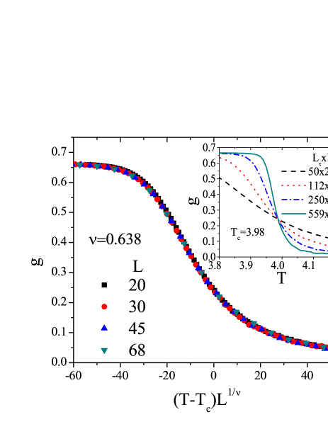
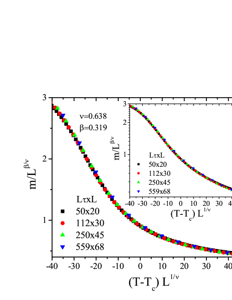
Both quantities display high-quality scaling as does the susceptibility (not shown). The resulting critical exponents, $\nu=0.638$, $z=1.98$, $\beta=0.319$, and $\gamma=1.27$ agree with literature values for the dissipative transverse-field Ising chain.Werner et al. (2005)

We note that the correlation length exponent violates the Harris criterionHarris (1974) $d_{\perp}\nu>2$. Here, $d_{\perp}=1$ is the number of “random dimensions” which differs from the total dimensionality $d=2$ of the classical model (7) because the disorder is perfectly correlated in the time-like direction. The violation of Harris’ inequality suggests that weak disorder is a relevant perturbation at the clean critical point; the character of the transition is thus expected to change upon the introduction of disorder.

In addition to providing a test of our numerical algorithm, the clean system simulations also give us a value for the upper Griffiths temperature $T_{u}$ for later use in the analysis of the disordered case. The upper Griffiths temperature is the temperature above which no (rare) locally ordered regions can exist in the disordered system. For the binary disorder distribution (8), the upper Griffiths temperature is identical to the critical temperature of an impurity-free system ($p=0$). Thus, in our case $T_{u}=T_{c}^{0}\approx 3.98$.

We now turn to our simulations of the disordered case, using $p=0.8$ and $c=0.25$ in the binary distribution (8). To establish the smeared character of the phase transition, we analyzed the temperature dependence of the magnetization. According to the theoretical predictions,Vojta (2003a, b) the magnetization is expected to develop an exponential tail of the form

$$m=m_{0}\,\exp[-(T_{c}^{0}-T)^{-\nu}]$$ (9)

towards the upper Griffiths temperature $T_{u}=T_{c}^{0}$. Here, $\nu$ is the correlation length exponent of the clean system. This tail forms because sufficiently large individual rare regions undergo the phase transition independently at different values of the tuning parameter. (After the quantum-to-classical mapping, these rare regions correspond to “strips” of finite width in the space direction.) To see this phenomenon in the simulations of finite-size systems requires a careful choice of the simulation parameters. In particular, the system size $L_{\tau}$ in the time-like direction needs to be very large to allow for sharp transitions of the individual rare regions to occur. Note that the smeared transition in the original quantum Hamiltonian (1) occurs only in the zero-temperature limit which corresponds to the limit $L_{\tau}\to\infty$ in the classical model (7). In contrast, the system size $L$ is space direction is not very important because the tail of the smeared transition is produced by finite-size rare regions (and the spatial correlation length remains finite).

Figure 3 shows the magnetization as a function of temperature for a system of size $L=50,L_{\tau}=6000$, averaged over 200 disorder realizations.

Figure 3: (Color online) Magnetization $m$ vs temperature $T$ for the classical Hamiltonian (7) with $p=0.8$, $c=0.25$, $\bar{\alpha}=1$ and $J^{\tau}=0$ for a system of size $L=50,L_{\tau}=6000$, averaged over 200 disorder realizations. $m$ develops a pronounced tail towards $T_{c}^{0}=3.98$. The solid line is a fit to (9). The semi-log plot of the same data in the inset shows that the theoretical prediction fits the tail region for almost two orders of magnitude in $m$.

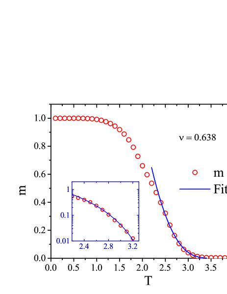
The data display a pronounced tail towards the upper Griffiths temperature $T_{u}=T_{c}^{0}$. We have compared different system sizes to ensure that this tail is not the result of any remaining finite-size effects. To compare with the theoretical predictions, we fit the magnetization in the tail region (temperatures above the inflection point at $T\approx 2.3$) to the exponential form (9). The numerical data follow the prediction for almost two orders of magnitude in $m$ (temperatures between 2.3 and 3.2). At higher temperatures, the numerical magnetization value is dominated by Monte-Carlo noise and thus saturates at a roughly temperature-independent value. (To suppress this effect, one would need to use even larger system sizes.)

In addition to the magnetization, we also studied the magnetic susceptibility in the tail region of the smeared transition. According to the strong-disorder renormalization group theory,Hoyos and Vojta (2008, 2012) the temperature dependence of the susceptibility of the quantum Hamiltonian (1) is characterized by a complicated double crossover (see Fig. 3b of Ref. Hoyos and Vojta, 2012). At higher temperatures, the physics is dominated by small clusters that cannot order (or freeze) independently. Thus, they display power-law quantum Griffiths behavior similar to the dissipationless system. At lower temperatures, the relevant clusters become large enough to undergo the localization phase transition independently, i.e., their quantum dynamics freezes. As a result, each such region makes a classical Curie contribution to the susceptibility.

Under the quantum-to-classical mapping, the (inverse) temperature in the quantum Hamiltonian (1) maps onto the time-like system size $L_{\tau}$ in the classical model (7). Figure 4 thus shows the dependence of the magnetic susceptibility $\chi$ on $L_{\tau}$ for several values of the classical temperature $T$ in the tail region of the smeared transition.

Figure 4: (Color online) Susceptibility $\chi$ vs system size $L_{\tau}$ for the classical Hamiltonian (7) with $p=0.8$, $c=0.25$, $J^{\tau}=0$, and $\bar{\alpha}=1$ at different values of the classical temperature $T$. The spatial system size is $L=3000$. The solid lines are fits to the power-law (10).

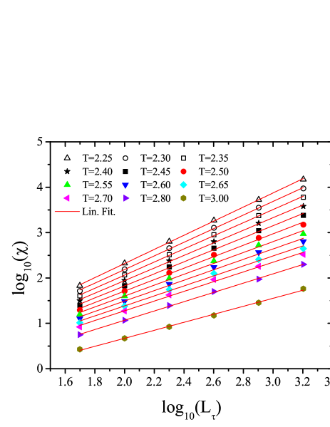
The data can all be fitted well by the power-law relation

$$\chi\sim L_{\tau}^{1-\lambda}=L_{\tau}^{1\pm 1/z^{\prime}}$$ (10)

where $\lambda$ is the usual nonuniversal Griffiths exponent (see, e.g., Ref. Vojta, 2006b) and $z^{\prime}$ is the corresponding dynamical exponent in the Griffiths phase. Here, the $+$ sign in the exponent applies in the ferromagnetic Griffiths phase and the $-$ sign in the paramagnetic Griffiths phase. For the fit curves in Fig. 4, $\lambda$ ranges from -0.55 at $T=2.25$ to 0.12 at $T=3.0$.

The fact that all data in Fig. 4 follow (pure) power laws with a monotonously changing exponent $\lambda$ suggests that our simulations are still in the transient Griffiths regime predicted by the strong-disorder renormalization group. They have not yet reached the asymptotic large-$L_{\tau}$ regime dominated by frozen clusters. In fact, the data at the highest classical temperature $T=3.0$ show a slight upturn for large $L_{\tau}$ which may indicate the beginning of the crossover to the asymptotic regime.

III.3 Crossover between the dissipationless and dissipative cases

The strong-disorder renormalization group theoryHoyos and Vojta (2008, 2012) also makes detailed predictions for the crossover from the dissipationless to the dissipative behavior with increasing dissipation strength $\alpha$. To investigate this crossover numerically, we first analyzed a dissipationless system by setting $\bar{\alpha}=0$ and $J^{\tau}=1$. In this case, the theory predicts a sharp transition governed by an infinite-randomness critical point.Fisher (1992, 1995) We confirmed this prediction by applying the methods of Ref. Hrahsheh et al., 2011 to the case at hand, in agreement with earlier simulation results in the literature.Young and Rieger (1996) Specifically, by analyzing the finite-size scaling properties of the susceptibility, we found the critical temperature of the dissipationless system to be $T_{c}^{dl}\approx 1.414$ (see Fig. 5).

Figure 5: (Color online) Griffiths dynamical exponent $z^{\prime}$ vs temperature $T$ for the classical Hamiltonian (7) with $p=0.8$, $c=0.25$, and $J^{\tau}=1$ in the absence of dissipation ($\bar{\alpha}=0)$. A fit to the expectedFisher (1995) power law $z^{\prime}\sim|T-T_{c}^{dl}|^{-1}$ results in $T_{c}^{dl}\approx 1.414$. The inset shows the raw susceptibility data as a function of the time-like system size $L_{\tau}$. The spatial system size is $L=2000$, and the data are averaged over 1400 to 2000 disorder realizations.

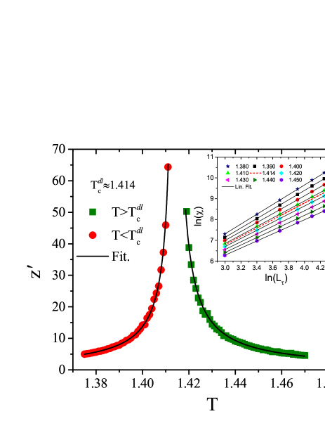
We then performed simulations for $J^{\tau}=1$ and several values of the dissipation strength between $\bar{\alpha}=0.01$ and 0.5. The resulting magnetization in the temperature range $T=1.0$ to 3.0 is presented in Fig. 6.

Figure 6: (Color online) Magnetization $m$ vs temperature $T$ for the classical Hamiltonian (7) with $p=0.8$, $c=0.25$, and $J^{\tau}=1$ for several values of the dissipation strength $\bar{\alpha}$. The system size is $L=200,L_{\tau}=10000$, and the data are averaged over 500 disorder realizations. The critical temperature of the dissipationless system ($\bar{\alpha}=0$) is $T_{c}^{dl}\approx 1.414$.

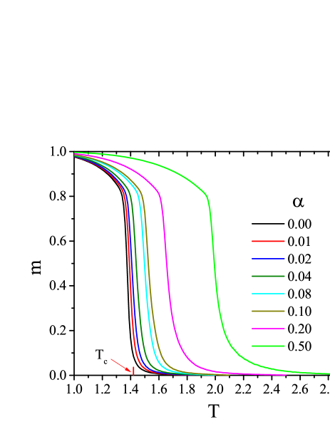
In this figure, even the magnetization of the dissipationless system ($\bar{\alpha}=0$), which has a sharp phase transition in the thermodynamic limit, shows a small “tail.” It stems from the remaining finite-size effects and can thus not be completely avoided. With increasing dissipation, the magnetization tail becomes much more pronounced than this finite-size tail, again lending support to the smeared transition scenario of Refs. Hoyos and Vojta, 2008, 2012.

However, a quantitative comparison with the theory of the crossover between the dissipationless and dissipative cases would require analyzing the weak-dissipation data ($\bar{\alpha}\ll 1$). For these cases, the smearing-induced magnetization tail is masked by the remaining finite-size effects and can thus not be studied quantitatively. Analogous problems also hinder the analysis of the magnetic susceptibility. We conclude that although our weak-dissipation results are in qualitative agreement with the theoretical predictions, a quantitative test of the crossover would require significantly larger systems.

IV Conclusions

To summarize, we investigated the quantum phase transition of a random transverse-field Ising chain in the presence of Ohmic dissipation. To this end, we first mapped the quantum Hamiltonian onto a classical two-dimensional Ising model with long-range ($1/\tau^{2}$) interactions in the time-like direction. This classical system was then studied by means of Monte-Carlo simulations using the Luijten/Blöte version of the Wolff cluster algorithm that efficiently deals with the long-range interactions.

Our results provide numerical evidence for the predictions of a recent strong-disorder renormalization group theoryHoyos and Vojta (2008, 2012) as well as earlier heuristic arguments.Vojta (2003a) In particular, the simulations confirm that the combined effects of disorder and dissipation lead to a destruction of the sharp quantum phase transition by smearing. This happens because different spatial regions can undergo the phase transition independently of the bulk system at different values of the tuning parameter.

For sufficiently strong dissipation (here, $\bar{\alpha}=1$), we could quantitatively compare the simulation data with the theoretical predictions and found them in good agreement. For weak dissipation, a quantitative comparison was not possible because the dissipation-induced tail of the smeared transition is small and thus masked by the remaining finite-size effects in our simulations.

As pointed out in the introduction, the renormalization group theoryHoyos and Vojta (2008, 2012) becomes controlled in the limit of strong randomness while its applicability to weak and moderate disorder requires independent verification. The binary distribution (8) used in our simulations constitutes moderate disorder, because $\Delta J^{x}/J^{x}$ is of order unity but the distribution is not broad on a logarithmic scale. Our simulations thus show that a moderately disordered system follows the predictions of the strong-disorder theory. Moreover, because the clean system violates the Harris criterion (see Sec. III.2) weak (bare) disorder will increase under coarse graining. This strongly suggests that the strong-disorder renormalization group theory governs the transition for any nonzero disorder strength. A direct numerical verification for weak disorder would be computationally expensive because the crossover to the disorder-dominated behavior would occur at very large system sizes only.

Both the renormalization group theory and the present simulations address the case of one space dimension. However, many applications of the smeared-transition scenario are actually in higher-dimensional systems. It is thus useful to discuss what changes in higher dimensions. The most important insight is that the smearing of the transition is driven by the freezing of individual finite-size regions of the sample. This implies that the space dimensionality does not play an important role. We thus expect that the same smeared-transition scenario applies in all dimensions. To test this numerically, one could map the $d$-dimensional dissipative random transverse-field Ising model to a $(d+1)$-dimensional version of the classical Hamiltonian (7) and then apply the methods of this paper. Generalizations to other types of dissipation (subohmic and superohmic) are also straight forward, they simply lead to different power-laws in the long-range interaction in the classical Hamiltonian (7). The Luijten-Blöte algorithmLuijten and Blöte (1995) can be applied in all of these cases.

The most important experimental realizations of smeared quantum phase transitions can arguably be found in disordered metallic magnets. The standard approach to magnetic quantum phase transitions in Fermi liquidsHertz (1976); Millis (1993) leads to an order-parameter field theory with a structure similar to our classical Hamiltonian (7). In particular, the order-parameter fluctuations experience Ohmic damping reflected in a long-range $1/\tau^{2}$ interaction in the imaginary time direction. Recently, indications of frozen local clusters have been observedUbaid-Kassis et al. (2010); Schroeder et al. (2011) near the ferromagnetic quantum phase transition in ${\mathrm{Ni}}_{1-x}{\mathrm{V}}_{x}$. Moreover, the ferromagnetic quantum phase transition in ${\mathrm{Sr}}_{1-x}{\mathrm{Ca}}_{x}{\mathrm{RuO}}_{3}$ was shown to be smeared by the disorder introduced via the Ca substitution.Demkó et al. (2012)

References

- Leggett et al. (1987) A. J. Leggett, S. Chakravarty, A. T. Dorsey, M. P. A. Fisher, A. Garg, and W. Zwerger, Rev. Mod. Phys. 59, 1 (1987).
- Weiss (1993) U. Weiss, Quantum disspative systems (World Scientific, Singapore, 1993).
- Vojta (2006a) M. Vojta, Phil. Mag. 86, 1807 (2006a).
- Werner et al. (2005) P. Werner, K. Völker, M. Troyer, and S. Chakravarty, Phys. Rev. Lett. 94, 047201 (2005).
- Hertz (1976) J. Hertz, Phys. Rev. B 14, 1165 (1976).
- Millis (1993) A. J. Millis, Phys. Rev. B 48, 7183 (1993).
- von Löhneysen et al. (2007) H. von Löhneysen, A. Rosch, M. Vojta, and P. Wölfle, Rev. Mod. Phys. 79, 1015 (2007).
- Imry and Wortis (1979) Y. Imry and M. Wortis, Phys. Rev. B 19, 3580 (1979).
- Hui and Berker (1989) K. Hui and A. N. Berker, Phys. Rev. Lett. 62, 2507 (1989).
- Aizenman and Wehr (1989) M. Aizenman and J. Wehr, Phys. Rev. Lett. 62, 2503 (1989).
- Greenblatt et al. (2009) R. L. Greenblatt, M. Aizenman, and J. L. Lebowitz, Phys. Rev. Lett. 103, 197201 (2009).
- Harris (1974) A. B. Harris, J. Phys. C 7, 1671 (1974).
- Fisher (1992) D. S. Fisher, Phys. Rev. Lett. 69, 534 (1992).
- Fisher (1995) D. S. Fisher, Phys. Rev. B 51, 6411 (1995).
- Thill and Huse (1995) M. Thill and D. A. Huse, Physica A 214, 321 (1995).
- Rieger and Young (1996) H. Rieger and A. P. Young, Phys. Rev. B 54, 3328 (1996).
- Vojta (2006b) T. Vojta, J. Phys. A 39, R143 (2006b).
- Vojta (2010) T. Vojta, J. Low Temp. Phys. 161, 299 (2010).
- Vojta (2003a) T. Vojta, Phys. Rev. Lett. 90, 107202 (2003a).
- Schehr and Rieger (2006) G. Schehr and H. Rieger, Phys. Rev. Lett. 96, 227201 (2006).
- Schehr and Rieger (2008) G. Schehr and H. Rieger, J. Stat. Mech. 2008, P04012 (2008).
- Hoyos and Vojta (2008) J. A. Hoyos and T. Vojta, Phys. Rev. Lett. 100, 240601 (2008).
- Hoyos and Vojta (2012) J. A. Hoyos and T. Vojta, Phys. Rev. B 85, 174403 (2012).
- Feynman and Hibbs (1965) R. P. Feynman and A. R. Hibbs, Quantum Mechanics and Path Integrals (McGraw-Hill, New York, 1965).
- Sachdev (1999) S. Sachdev, Quantum phase transitions (Cambridge University Press, Cambridge, 1999).
- Wolff (1989) U. Wolff, Phys. Rev. Lett. 62, 361 (1989).
- Luijten and Blöte (1995) E. Luijten and H. W. J. Blöte, Int. J. Mod. Phys. C 6, 359 (1995).
- Vojta (2003b) T. Vojta, J. Phys. A 36, 10921 (2003b).
- Hrahsheh et al. (2011) F. Hrahsheh, H. Barghathi, and T. Vojta, Phys. Rev. B 84, 184202 (2011).
- Young and Rieger (1996) A. P. Young and H. Rieger, Phys. Rev. B 53, 8486 (1996).
- Ubaid-Kassis et al. (2010) S. Ubaid-Kassis, T. Vojta, and A. Schroeder, Phys. Rev. Lett. 104, 066402 (2010).
- Schroeder et al. (2011) A. Schroeder, S. Ubaid-Kassis, and T. Vojta, J. Phys. Condes. Matter 23, 094205 (2011).
- Demkó et al. (2012) L. Demkó, S. Bordács, T. Vojta, D. Nozadze, F. Hrahsheh, C. Svoboda, B. Dóra, H. Yamada, M. Kawasaki, Y. Tokura, and I. Kézsmárki, Phys. Rev. Lett. 108, 185701 (2012).