IPMU-13-0143

KEK-TH-1641


Flavor of Gluino Decay in High-Scale Supersymmetry


Ryosuke Sato1, Satoshi Shirai2 and Kohsaku Tobioka3

1 Institute of Particle and Nuclear Studies,
High Energy Accelerator Research Organization (KEK)
Tsukuba 305-0801, Japan
2Berkeley Center for Theoretical Physics, Department of Physics,
and Theoretical Physics Group, Lawrence Berkeley National Laboratory,
University of California, Berkeley, CA 94720, USA
3Department of Physics, University of Tokyo, Tokyo 113-0033, Japan,
and Kavli Institute for the Physics and Mathematics of the Universe (WPI),
Todai Institutes for Advanced Study, University of Tokyo,
Kashiwa 277-8583, Japan


1 Introduction

A supersymmetric (SUSY) standard model (SSM) is a leading candidate of physics beyond the standard model (SM). However the most “natural” SUSY model suffers from long-standing problems, such as low-energy flavor/CP physics, direct sparticle search, Higgs boson mass, and cosmology. Many types of SSMs are studied to get over such difficulties.

The discovery of the 125 GeV Higgs boson [1, 2] indicates a possibility of a very simple framework of SSMs, i.e., high-scale SUSY scenarios [3, 4, 5, 6, 7]. The sfermion mass scale higher than 𝒪(10)𝒪10{\cal O}(10) TeV can explain for the 125 GeV Higgs boson [8, 9]. In addition, constraints of the SUSY flavor/CP problems and cosmological problems are greatly relaxed. As for the fermion sectors, the R-parity conservation sets gauginos and/or Higgsino mass scale to a TeV range to avoid the dark matter overabundance, which is also preferred by the gauge coupling unification. From a theoretical viewpoint, such a setup can be simply realized. For example, an assumption of some charge of the SUSY breaking field X𝑋X leads the sfermion mass msfermion>m3/2superscriptsubscriptsubscript𝑚sfermionsimilar-tosubscript𝑚32m_{\rm sfermion}\mathop{}_{\textstyle\sim}^{\textstyle>}m_{3/2}, keeping the gauginos light, mgaugino0.01m3/2similar-tosubscript𝑚gaugino0.01subscript𝑚32m_{\rm gaugino}\sim 0.01m_{3/2}, which are generated via anomaly mediation effects [10]. By setting m3/2=𝒪(1023)subscript𝑚32𝒪superscript1023m_{3/2}={\cal O}(10^{2-3}) TeV, a viable SUSY mass spectrum can be obtained. After the discovery of the Higgs boson, such a framework gets more attention, variously called “Spread SUSY” [11], “Pure Gravity Mediation” [12], “Mini-Split” [13], “Simply Unnatural SUSY” [14] and so on. This framework predicts a Wino is the lightest SUSY particle (LSP). There are intensive studies of collider [15, 16] and dark matter [17, 18, 19, 20, 21, 22, 23] signals of the Wino LSP.

Such a large mass hierarchy the between gaugino and scalar sector is not an uncommon feature of SUSY breaking models. This is because the mass of fermions can be protected from large radiative corrections thanks to some chiral symmetry and, on the other hand, that of the scalar particle is not protected, once SUSY is broken. For example, the large mass hierarchy also exists in some class of gauge mediated SUSY breaking (GMSB) models. See, e.g., Refs. [24, 25] for such models. This feature quite often comes from underlying symmetry of the model and/or stability conditions of the SUSY breaking vacua [26, 27]. Motivated by the discovery of the Higgs boson, such GMSB models also have been studied [13, 28].

Several kinds of SUSY breaking models realize the high-scale SUSY spectrum. Although they predict similar spectra at a TeV scale, the gravitino mass and sfermion sector have strong model dependence. One of the characteristic features of each model appears in the sfermion sector. For example, without any flavor symmetry, we can expect flavor violating soft parameters of the order of the scalar mass scale. On the other hand, some flavor symmetry forbid such terms, depending on the symmetry charge assignments. Or a typical GMSB model predicts just the minimal flavor violation. A grand unified theory (GUT) may determine the mass relation among the sfermion sector. Therefore, probing the sfermion sector is essential to study the underlying model. The information on the sfermion sector is also important for us to discuss the prospects of precise measurements of flavor/CP experiments.

For the future flavor/CP observations and deeper understanding the underlying theory of the high-scale SUSY models, it is very important to know the property of the sfermion sector, such as its mass scale and flavor structure. Since the direct production of heavy sfermions is out of range of the LHC, we must consider indirect ways to probe the sfermion sector. A cosmological signature such as gravitational waves is an interesting possibility among them [29]. Another possibility is the gluino decay since it is sensitive to the squark sector. The most known feature of the gluino in the high-scale SUSY models is its longevity of the lifetime. Another interesting point is that the flavor violating decay modes of the gluino are allowed thanks to heavy squark masses satisfying flavor constraints for the SM particles. Hence, by studying the gluino decay in detail, we can get insights into the squark sectors. In this paper we study the gluino decay in the high-scale SUSY models.

For heavy squarks, quantum corrections to the gluino decay get large, and can significantly affect the gluino decay, compared to the tree-level calculation. Previously, there are some works to study the tree-level gluino decay with flavor/CP violation [30] and the quantum effect without flavor/CP violation in the high-scale SUSY models [31, 32]. In this study, we pay particular attention to the quantum effects on the flavor structure of the gluino decay and discuss the correlation with the low-energy flavor/CP violating rare processes. In section 2, we estimate the size of the quantum corrections for the gluino decay, using renormalization group equations. In section 3, we discuss the correlation between the low-energy flavor/CP observations and the gluino decay. In section 4, we briefly discuss the collider signatures. Section 5 is devoted to summary and discussions.

2 Gluino Decay in High-scale SUSY Models

In the high-scale SUSY models, we cannot directly probe the sfermions at the LHC. However, the gluino decay requires virtual squark exchanges and therefore it reflects the squark sector. The most significant feature of the high-scale SUSY model is the longevity of the gluino lifetime since, as the squark mass scale goes high, the lifetime of the gluino can be very long. Typically, its decay length is cτg~1cm(mq~/1000TeV)4(mg~/1TeV)5similar-to𝑐subscript𝜏~𝑔1cmsuperscriptsubscript𝑚~𝑞1000TeV4superscriptsubscript𝑚~𝑔1TeV5c\tau_{\tilde{g}}\sim 1~{}{\rm cm}(m_{\tilde{q}}/1000~{}{\rm TeV})^{4}(m_{\tilde{g}}/1~{}{\rm TeV})^{-5}. Such a long lifetime plays a significant role not only in collier signals but also in cosmology. Cosmological constraints disfavor the gluino lifetime much longer than 1 sec [33].

Another important feature is that the decay products of the gluino carry information on details of the squark flavor structure. For instance, if the third family squarks are lighter than the other squarks, the final states of the gluino decay are rich in bottom and top quarks. Furthermore, with the flavor violating structure of the squarks, we may observe the flavor violating gluino decay. In this way, the squark sector is testable via the gluino decay. To extract information on the sfermion sector via observation of the gluino decay, we need to sophisticate a prediction of the gluino decay, including quantum corrections.

In this section, we calculate partial decay widths of the gluino by a renormalization group (RG) method. We study the RG evolution of Wilson coefficients that govern the gluino decay with general flavor/CP structure and see the effects on the gluino decay.

2.1 Effective Theory and RG Equations of Wilson Coefficients

We assume that sfermions, heavy Higgs bosons and Higgsinos have the masses of around m~>𝒪(10)TeV~𝑚𝒪10TeV\tilde{m}>{\cal O}(10)~{}{\rm TeV} and that the size of A𝐴A-terms is negligible. The soft mass terms relevant to our study are

soft=12(mB~B~B~+mW~W~AW~A+mg~g~ag~a+h.c.)Q~LmQ~L2Q~Lu~Rcmu~R2u~Rcd~Rcmd~R2d~Rc,\displaystyle{\cal L}_{\rm soft}=-\frac{1}{2}\left(m_{\tilde{B}}\tilde{B}\tilde{B}+m_{\tilde{W}}\tilde{W}^{A}\tilde{W}^{A}+m_{\tilde{g}}\tilde{g}^{a}\tilde{g}^{a}+h.c.\right)-{\tilde{Q}_{L}}^{*}m^{2}_{\tilde{Q}_{L}}{\tilde{Q}_{L}}-{\tilde{u}_{R}}^{c}m^{2}_{\tilde{u}_{R}}{\tilde{u}_{R}^{c*}}-{\tilde{d}_{R}}^{c}m^{2}_{\tilde{d}_{R}}{\tilde{d}_{R}^{c*}}, (1)

where mB~subscript𝑚~𝐵m_{\tilde{B}}, mW~subscript𝑚~𝑊m_{\tilde{W}} and mg~subscript𝑚~𝑔m_{\tilde{g}} are complex gaugino masses and mQ~L2subscriptsuperscript𝑚2subscript~𝑄𝐿m^{2}_{\tilde{Q}_{L}}, mu~R2subscriptsuperscript𝑚2subscript~𝑢𝑅m^{2}_{\tilde{u}_{R}} and md~R2subscriptsuperscript𝑚2subscript~𝑑𝑅m^{2}_{\tilde{d}_{R}} are 3×3333\times 3 Hermitian matrices whose components are 𝒪(m~2)𝒪superscript~𝑚2{\cal O}(\tilde{m}^{2}). In this section, we take weak basis in which QL,isubscript𝑄𝐿𝑖Q_{L,i} and Q~L,isubscript~𝑄𝐿𝑖\tilde{Q}_{L,i} form an SU(2)L𝑆𝑈subscript2𝐿SU(2)_{L} doublet for each i𝑖i. Thanks to this notation, we can write effective interactions and RG equations for their Wilson coefficients as SU(2)L𝑆𝑈subscript2𝐿SU(2)_{L} symmetric forms. For a detail, see the Appendix A.

Below the scale m~~𝑚\tilde{m}, the dynamics of the particles is described by an effective theory which contains the SM particles and gauginos. The gluino will mainly decay into a lighter SUSY particle by emitting two quarks or a gluon. These decay modes are dominantly induced by the following dimension five and six effective interactions by integrating out the heavy squarks:

QQ,ijB~superscriptsubscript𝑄𝑄𝑖𝑗~𝐵\displaystyle Q_{Q,ij}^{\tilde{B}} =\displaystyle= (B~σ¯μg~a)(QL,iσ¯μTaQL,j),superscript~𝐵superscript¯𝜎𝜇superscript~𝑔𝑎superscriptsubscript𝑄𝐿𝑖subscript¯𝜎𝜇superscript𝑇𝑎subscript𝑄𝐿𝑗\displaystyle(\tilde{B}^{\dagger}\bar{\sigma}^{\mu}\tilde{g}^{a})(Q_{L,i}^{\dagger}\bar{\sigma}_{\mu}T^{a}Q_{L,j}), (2)
Qu,ijB~superscriptsubscript𝑄𝑢𝑖𝑗~𝐵\displaystyle Q_{u,ij}^{\tilde{B}} =\displaystyle= (B~σ¯μg~a)(uR,icσμTauR,jc),superscript~𝐵superscript¯𝜎𝜇superscript~𝑔𝑎superscriptsubscript𝑢𝑅𝑖𝑐subscript𝜎𝜇superscript𝑇𝑎superscriptsubscript𝑢𝑅𝑗𝑐\displaystyle(\tilde{B}^{\dagger}\bar{\sigma}^{\mu}\tilde{g}^{a})(u_{R,i}^{c}\sigma_{\mu}T^{a}u_{R,j}^{c\dagger}), (3)
Qd,ijB~superscriptsubscript𝑄𝑑𝑖𝑗~𝐵\displaystyle Q_{d,ij}^{\tilde{B}} =\displaystyle= (B~σ¯μg~a)(dR,icσμTadR,jc),superscript~𝐵superscript¯𝜎𝜇superscript~𝑔𝑎superscriptsubscript𝑑𝑅𝑖𝑐subscript𝜎𝜇superscript𝑇𝑎superscriptsubscript𝑑𝑅𝑗𝑐\displaystyle(\tilde{B}^{\dagger}\bar{\sigma}^{\mu}\tilde{g}^{a})(d_{R,i}^{c}\sigma_{\mu}T^{a}d_{R,j}^{c\dagger}), (4)
Q7B~superscriptsubscript𝑄7~𝐵\displaystyle Q_{7}^{\tilde{B}} =\displaystyle= (B~σ¯μνg~a)Gμνa,~𝐵superscript¯𝜎𝜇𝜈superscript~𝑔𝑎subscriptsuperscript𝐺𝑎𝜇𝜈\displaystyle(\tilde{B}\bar{\sigma}^{\mu\nu}\tilde{g}^{a})G^{a}_{\mu\nu}, (5)
QijW~superscriptsubscript𝑄𝑖𝑗~𝑊\displaystyle Q_{ij}^{\tilde{W}} =\displaystyle= (W~Aσ¯μg~a)(QL,iσ¯μTaτAQL,j).superscript~𝑊𝐴superscript¯𝜎𝜇superscript~𝑔𝑎superscriptsubscript𝑄𝐿𝑖subscript¯𝜎𝜇superscript𝑇𝑎superscript𝜏𝐴subscript𝑄𝐿𝑗\displaystyle(\tilde{W}^{A\dagger}\bar{\sigma}^{\mu}\tilde{g}^{a})(Q_{L,i}^{\dagger}\bar{\sigma}_{\mu}T^{a}\tau^{A}Q_{L,j}). (6)

Here, i,j=1,2,3formulae-sequence𝑖𝑗123i,j=1,2,3 are flavor indices, A=1,2,3𝐴123A=1,2,3 is an SU(2)L𝑆𝑈subscript2𝐿SU(2)_{L} adjoint index and a=1,,8𝑎18a=1,\cdots,8 is an SU(3)C𝑆𝑈subscript3𝐶SU(3)_{C} adjoint index.

The effective Lagrangian contains the following interaction terms:

eff.=1m~2[i=13j=13(CQ,ijB~QQ,ijB~+Cu,ijB~Qu,ijB~+Cd,ijB~Qd,ijB~+CijW~QijW~)+C7B~Q7B~]+h.c..formulae-sequencesubscripteff1superscript~𝑚2delimited-[]superscriptsubscript𝑖13superscriptsubscript𝑗13subscriptsuperscript𝐶~𝐵𝑄𝑖𝑗subscriptsuperscript𝑄~𝐵𝑄𝑖𝑗subscriptsuperscript𝐶~𝐵𝑢𝑖𝑗subscriptsuperscript𝑄~𝐵𝑢𝑖𝑗subscriptsuperscript𝐶~𝐵𝑑𝑖𝑗subscriptsuperscript𝑄~𝐵𝑑𝑖𝑗subscriptsuperscript𝐶~𝑊𝑖𝑗subscriptsuperscript𝑄~𝑊𝑖𝑗subscriptsuperscript𝐶~𝐵7subscriptsuperscript𝑄~𝐵7𝑐\displaystyle{\cal L}_{\rm eff.}~{}=~{}\frac{1}{\tilde{m}^{2}}\left[\sum_{i=1}^{3}\sum_{j=1}^{3}\left(C^{\tilde{B}}_{Q,ij}Q^{\tilde{B}}_{Q,ij}+C^{\tilde{B}}_{u,ij}Q^{\tilde{B}}_{u,ij}+C^{\tilde{B}}_{d,ij}Q^{\tilde{B}}_{d,ij}+C^{\tilde{W}}_{ij}Q^{\tilde{W}}_{ij}\right)+C^{\tilde{B}}_{7}Q^{\tilde{B}}_{7}\right]+h.c.. (7)

Boundary condition at the squark mass scale

We have to match our effective theory with the MSSM at the squark mass scale m~~𝑚\tilde{m}. The Wilson coefficients C(m~)𝐶~𝑚C(\tilde{m})’s are obtained by integrating out the squarks. At the leading order, we obtain,

CQ,ijB~(m~)subscriptsuperscript𝐶~𝐵𝑄𝑖𝑗~𝑚\displaystyle C^{\tilde{B}}_{Q,ij}(\tilde{m}) =\displaystyle= gsg6m~2(mQ~L2)ij1,subscript𝑔𝑠superscript𝑔6superscript~𝑚2subscriptsuperscriptsubscriptsuperscript𝑚2subscript~𝑄𝐿1𝑖𝑗\displaystyle-\frac{g_{s}g^{\prime}}{6}\tilde{m}^{2}(m^{2}_{\tilde{Q}_{L}})^{-1}_{ij}, (8)
Cu,ijB~(m~)subscriptsuperscript𝐶~𝐵𝑢𝑖𝑗~𝑚\displaystyle C^{\tilde{B}}_{u,ij}(\tilde{m}) =\displaystyle= 2gsg3m~2(mu~R2)ji1,2subscript𝑔𝑠superscript𝑔3superscript~𝑚2subscriptsuperscriptsubscriptsuperscript𝑚2subscript~𝑢𝑅1𝑗𝑖\displaystyle\frac{2g_{s}g^{\prime}}{3}\tilde{m}^{2}(m^{2}_{\tilde{u}_{R}})^{-1}_{ji}, (9)
Cd,ijB~(m~)subscriptsuperscript𝐶~𝐵𝑑𝑖𝑗~𝑚\displaystyle C^{\tilde{B}}_{d,ij}(\tilde{m}) =\displaystyle= gsg3m~2(md~R2)ji1,subscript𝑔𝑠superscript𝑔3superscript~𝑚2subscriptsuperscriptsubscriptsuperscript𝑚2subscript~𝑑𝑅1𝑗𝑖\displaystyle-\frac{g_{s}g^{\prime}}{3}\tilde{m}^{2}(m^{2}_{\tilde{d}_{R}})^{-1}_{ji}, (10)
C7B~(m~)subscriptsuperscript𝐶~𝐵7~𝑚\displaystyle C^{\tilde{B}}_{7}(\tilde{m}) =\displaystyle= gs2g384π2(mg~mB~)m~2(tr[(mQ~L2)1]2tr[(mu~R2)1]+tr[(md~R2)1]),superscriptsubscript𝑔𝑠2superscript𝑔384superscript𝜋2subscript𝑚~𝑔subscript𝑚~𝐵superscript~𝑚2trdelimited-[]superscriptsubscriptsuperscript𝑚2subscript~𝑄𝐿12trdelimited-[]superscriptsubscriptsuperscript𝑚2subscript~𝑢𝑅1trdelimited-[]superscriptsubscriptsuperscript𝑚2subscript~𝑑𝑅1\displaystyle\frac{g_{s}^{2}g^{\prime}}{384\pi^{2}}(m_{\tilde{g}}-m_{\tilde{B}})\tilde{m}^{2}\left({\rm tr}[(m^{2}_{\tilde{Q}_{L}})^{-1}]-2{\rm tr}[(m^{2}_{\tilde{u}_{R}})^{-1}]+{\rm tr}[(m^{2}_{\tilde{d}_{R}})^{-1}]\right), (11)
CijW~(m~)subscriptsuperscript𝐶~𝑊𝑖𝑗~𝑚\displaystyle C^{\tilde{W}}_{ij}(\tilde{m}) =\displaystyle= gsg2m~2(mQ~L2)ij1.subscript𝑔𝑠𝑔2superscript~𝑚2subscriptsuperscriptsubscriptsuperscript𝑚2subscript~𝑄𝐿1𝑖𝑗\displaystyle-\frac{g_{s}g}{2}\tilde{m}^{2}(m^{2}_{\tilde{Q}_{L}})^{-1}_{ij}. (12)

Here, mQ~L2superscriptsubscript𝑚subscript~𝑄𝐿2m_{\tilde{Q}_{L}}^{2}, mu~R2superscriptsubscript𝑚subscript~𝑢𝑅2m_{\tilde{u}_{R}}^{2} and md~R2superscriptsubscript𝑚subscript~𝑑𝑅2m_{\tilde{d}_{R}}^{2} are the squark mass-squared matrices at the scale m~~𝑚\tilde{m}. We treat the Wilson coefficients CQB~subscriptsuperscript𝐶~𝐵𝑄C^{\tilde{B}}_{Q}, CuB~subscriptsuperscript𝐶~𝐵𝑢C^{\tilde{B}}_{u}, CdB~subscriptsuperscript𝐶~𝐵𝑑C^{\tilde{B}}_{d} and CW~superscript𝐶~𝑊C^{\tilde{W}} as 3×3333\times 3 matrices in flavor space. In the high-scale SUSY models, there is a large hierarchy between the gaugino mass scale and the squark mass scale m~~𝑚\tilde{m}. Therefore, the resummation of leading logarithm corrections becomes important.

RG equations for Wilson coefficients
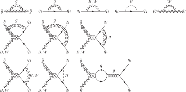
Refer to caption
Figure 1: One-loop diagrams for the anomalous dimensions of quarks and gauginos (top) and the anomalous dimensions of operators and operator mixings (middle and bottom).

Now, we describe the RG evolution of the Wilson coefficients at one-loop level. We treat SM-like Yukawa couplings Yusubscript𝑌𝑢Y_{u} and Ydsubscript𝑌𝑑Y_{d} as 3×3333\times 3 matrices in flavor space. They are defined as,

yukawa=HQLYuuRc+HQLYddRc+h.c..formulae-sequencesubscriptyukawa𝐻subscript𝑄𝐿subscript𝑌𝑢superscriptsubscript𝑢𝑅𝑐superscript𝐻subscript𝑄𝐿subscript𝑌𝑑superscriptsubscript𝑑𝑅𝑐𝑐\displaystyle{\cal L}_{\rm yukawa}=HQ_{L}Y_{u}u_{R}^{c}+H^{*}Q_{L}Y_{d}d_{R}^{c}+h.c.. (13)

Here, H𝐻H is the SM-like Higgs doublet field. RG equations for the gauge coupling constants are given by,

16π2dgdlogμ=416g3,16π2dgdlogμ=116g3,16π2dgsdlogμ=5gs3.formulae-sequence16superscript𝜋2𝑑superscript𝑔𝑑𝜇416superscript𝑔3formulae-sequence16superscript𝜋2𝑑𝑔𝑑𝜇116superscript𝑔316superscript𝜋2𝑑subscript𝑔𝑠𝑑𝜇5superscriptsubscript𝑔𝑠3\displaystyle 16\pi^{2}\frac{dg^{\prime}}{d\log\mu}~{}=~{}\frac{41}{6}g^{\prime 3},~{}~{}~{}~{}~{}16\pi^{2}\frac{dg}{d\log\mu}~{}=~{}-\frac{11}{6}g^{3},~{}~{}~{}~{}~{}16\pi^{2}\frac{dg_{s}}{d\log\mu}~{}=~{}-5g_{s}^{3}. (14)

For the quark Yukawa couplings,

16π2dYudlogμ16superscript𝜋2𝑑subscript𝑌𝑢𝑑𝜇\displaystyle 16\pi^{2}\frac{dY_{u}}{d\log\mu} =[32YuYu32YdYd+3tr(YuYu+YdYd)1712g294g228gs2]Yu,absentdelimited-[]32subscript𝑌𝑢superscriptsubscript𝑌𝑢32subscript𝑌𝑑superscriptsubscript𝑌𝑑3trsubscript𝑌𝑢superscriptsubscript𝑌𝑢subscript𝑌𝑑superscriptsubscript𝑌𝑑1712superscript𝑔294superscriptsubscript𝑔228superscriptsubscript𝑔𝑠2subscript𝑌𝑢\displaystyle=\left[\frac{3}{2}Y_{u}Y_{u}^{\dagger}-\frac{3}{2}Y_{d}Y_{d}^{\dagger}+3{\mathop{\rm tr}}\left(Y_{u}Y_{u}^{\dagger}+Y_{d}Y_{d}^{\dagger}\right)-\frac{17}{12}g^{\prime 2}-\frac{9}{4}g_{2}^{2}-8g_{s}^{2}\right]Y_{u}, (15)
16π2dYddlogμ16superscript𝜋2𝑑subscript𝑌𝑑𝑑𝜇\displaystyle 16\pi^{2}\frac{dY_{d}}{d\log\mu} =[32YuYu+32YdYd+3tr(YuYu+YdYd)512g294g228gs2]Yd.absentdelimited-[]32subscript𝑌𝑢superscriptsubscript𝑌𝑢32subscript𝑌𝑑superscriptsubscript𝑌𝑑3trsubscript𝑌𝑢superscriptsubscript𝑌𝑢subscript𝑌𝑑superscriptsubscript𝑌𝑑512superscript𝑔294superscriptsubscript𝑔228superscriptsubscript𝑔𝑠2subscript𝑌𝑑\displaystyle=\left[-\frac{3}{2}Y_{u}Y_{u}^{\dagger}+\frac{3}{2}Y_{d}Y_{d}^{\dagger}+3{\mathop{\rm tr}}\left(Y_{u}Y_{u}^{\dagger}+Y_{d}Y_{d}^{\dagger}\right)-\frac{5}{12}g^{\prime 2}-\frac{9}{4}g_{2}^{2}-8g_{s}^{2}\right]Y_{d}. (16)

Here, we neglect the lepton Yukawa interactions. The RG equations for gsuperscript𝑔g^{\prime}, Yusubscript𝑌𝑢Y_{u} and Ydsubscript𝑌𝑑Y_{d} at one-loop level are same as the SM ones [34]. RG equations for the Wilson coefficients are given by,111 One may worry about mixing with other operators, such as, dabc(B~σ¯μg~a)(g~bσ¯μg~c)subscript𝑑𝑎𝑏𝑐superscript~𝐵superscript¯𝜎𝜇superscript~𝑔𝑎superscript~𝑔𝑏subscript¯𝜎𝜇superscript~𝑔𝑐d_{abc}({\tilde{B}}^{\dagger}\bar{\sigma}^{\mu}\tilde{g}^{a})({\tilde{g}}^{b\dagger}\bar{\sigma}_{\mu}\tilde{g}^{c}) and dabc(B~g~a)(g~bg~c)subscript𝑑𝑎𝑏𝑐~𝐵superscript~𝑔𝑎superscript~𝑔𝑏superscript~𝑔𝑐d_{abc}({\tilde{B}}\tilde{g}^{a})({\tilde{g}}^{b}\tilde{g}^{c}). Here, dabc=tr[Ta{Tb,Tc}]subscript𝑑𝑎𝑏𝑐trdelimited-[]superscript𝑇𝑎superscript𝑇𝑏superscript𝑇𝑐d_{abc}={\rm tr}[T^{a}\{T^{b},T^{c}\}]. However, QQ,ijB~superscriptsubscript𝑄𝑄𝑖𝑗~𝐵Q_{Q,ij}^{\tilde{B}}, Qu,ijB~superscriptsubscript𝑄𝑢𝑖𝑗~𝐵Q_{u,ij}^{\tilde{B}}, Qd,ijB~superscriptsubscript𝑄𝑑𝑖𝑗~𝐵Q_{d,ij}^{\tilde{B}} and Q7B~superscriptsubscript𝑄7~𝐵Q_{7}^{\tilde{B}} do not mix with them at one-loop level.

16π2dCQB~dlogμ16superscript𝜋2𝑑subscriptsuperscript𝐶~𝐵𝑄𝑑𝜇\displaystyle 16\pi^{2}\frac{dC^{\tilde{B}}_{Q}}{d\log\mu} =12{YuYu+YdYd,CQB~}YuCuB~YuYdCdB~Yd3gs2NCCQB~+23gs2𝐒^,absent12subscript𝑌𝑢superscriptsubscript𝑌𝑢subscript𝑌𝑑superscriptsubscript𝑌𝑑subscriptsuperscript𝐶~𝐵𝑄subscript𝑌𝑢subscriptsuperscript𝐶~𝐵𝑢superscriptsubscript𝑌𝑢subscript𝑌𝑑subscriptsuperscript𝐶~𝐵𝑑superscriptsubscript𝑌𝑑3superscriptsubscript𝑔𝑠2subscript𝑁𝐶subscriptsuperscript𝐶~𝐵𝑄23superscriptsubscript𝑔𝑠2^𝐒\displaystyle=\frac{1}{2}\left\{Y_{u}Y_{u}^{\dagger}+Y_{d}Y_{d}^{\dagger},C^{\tilde{B}}_{Q}\right\}-Y_{u}C^{\tilde{B}}_{u}Y_{u}^{\dagger}-Y_{d}C^{\tilde{B}}_{d}Y_{d}^{\dagger}-3g_{s}^{2}N_{C}C^{\tilde{B}}_{Q}+\frac{2}{3}g_{s}^{2}\hat{\bf S}, (17)
16π2dCuB~dlogμ16superscript𝜋2𝑑subscriptsuperscript𝐶~𝐵𝑢𝑑𝜇\displaystyle 16\pi^{2}\frac{dC^{\tilde{B}}_{u}}{d\log\mu} ={YuYu,CuB~}2YuCQB~Yu3gs2NCCuB~+23gs2𝐒^,absentsuperscriptsubscript𝑌𝑢subscript𝑌𝑢subscriptsuperscript𝐶~𝐵𝑢2superscriptsubscript𝑌𝑢subscriptsuperscript𝐶~𝐵𝑄subscript𝑌𝑢3superscriptsubscript𝑔𝑠2subscript𝑁𝐶subscriptsuperscript𝐶~𝐵𝑢23superscriptsubscript𝑔𝑠2^𝐒\displaystyle=\left\{Y_{u}^{\dagger}Y_{u},C^{\tilde{B}}_{u}\right\}-2Y_{u}^{\dagger}C^{\tilde{B}}_{Q}Y_{u}-3g_{s}^{2}N_{C}C^{\tilde{B}}_{u}+\frac{2}{3}g_{s}^{2}\hat{\bf S}, (18)
16π2dCdB~dlogμ16superscript𝜋2𝑑subscriptsuperscript𝐶~𝐵𝑑𝑑𝜇\displaystyle 16\pi^{2}\frac{dC^{\tilde{B}}_{d}}{d\log\mu} ={YdYd,CdB~}2YdCQB~Yd3gs2NCCdB~+23gs2𝐒^,absentsuperscriptsubscript𝑌𝑑subscript𝑌𝑑subscriptsuperscript𝐶~𝐵𝑑2superscriptsubscript𝑌𝑑subscriptsuperscript𝐶~𝐵𝑄subscript𝑌𝑑3superscriptsubscript𝑔𝑠2subscript𝑁𝐶subscriptsuperscript𝐶~𝐵𝑑23superscriptsubscript𝑔𝑠2^𝐒\displaystyle=\left\{Y_{d}^{\dagger}Y_{d},C^{\tilde{B}}_{d}\right\}-2Y_{d}^{\dagger}C^{\tilde{B}}_{Q}Y_{d}-3g_{s}^{2}N_{C}C^{\tilde{B}}_{d}+\frac{2}{3}g_{s}^{2}\hat{\bf S}, (19)
16π2dC7B~dlogμ16superscript𝜋2𝑑subscriptsuperscript𝐶~𝐵7𝑑𝜇\displaystyle 16\pi^{2}\frac{dC^{\tilde{B}}_{7}}{d\log\mu} =(23NF6NC)gs2C7B~,absent23subscript𝑁𝐹6subscript𝑁𝐶superscriptsubscript𝑔𝑠2subscriptsuperscript𝐶~𝐵7\displaystyle=\left(\frac{2}{3}N_{F}-6N_{C}\right)g_{s}^{2}C^{\tilde{B}}_{7}, (20)
16π2dCW~dlogμ16superscript𝜋2𝑑superscript𝐶~𝑊𝑑𝜇\displaystyle 16\pi^{2}\frac{dC^{\tilde{W}}}{d\log\mu} =12{YuYu+YdYd,CW~}3gs2NCCW~6g2CW~.absent12subscript𝑌𝑢superscriptsubscript𝑌𝑢subscript𝑌𝑑superscriptsubscript𝑌𝑑superscript𝐶~𝑊3superscriptsubscript𝑔𝑠2subscript𝑁𝐶superscript𝐶~𝑊6superscript𝑔2superscript𝐶~𝑊\displaystyle=\frac{1}{2}\left\{Y_{u}Y_{u}^{\dagger}+Y_{d}Y_{d}^{\dagger},C^{\tilde{W}}\right\}-3g_{s}^{2}N_{C}C^{\tilde{W}}-6g^{2}C^{\tilde{W}}. (21)

Here, 𝐒^=(2trCQB~+trCuB~+trCdB~)𝟏^𝐒2trsubscriptsuperscript𝐶~𝐵𝑄trsubscriptsuperscript𝐶~𝐵𝑢trsubscriptsuperscript𝐶~𝐵𝑑1\hat{\bf S}=(2{\rm tr}C^{\tilde{B}}_{Q}+{\rm tr}C^{\tilde{B}}_{u}+{\rm tr}C^{\tilde{B}}_{d}){\bf 1}, {A,B}=AB+BA𝐴𝐵𝐴𝐵𝐵𝐴\{A,B\}=AB+BA, 𝟏=diag(1,1,1)1diag111{\bf 1}={\rm diag}(1,1,1), NF=6subscript𝑁𝐹6N_{F}=6 and NC=3subscript𝑁𝐶3N_{C}=3. Again, CQB~subscriptsuperscript𝐶~𝐵𝑄C^{\tilde{B}}_{Q}, CuB~subscriptsuperscript𝐶~𝐵𝑢C^{\tilde{B}}_{u}, CdB~subscriptsuperscript𝐶~𝐵𝑑C^{\tilde{B}}_{d} and CW~superscript𝐶~𝑊C^{\tilde{W}} are 3×3333\times 3 matrices in flavor space. We show one-loop diagrams which contribute to the above RG equations in Fig. 1. We have checked Eqs. (1721) are consistent with Ref. [31] in the flavor-symmetric case. 222 If the Higgsino is lighter than the gluino, we have to consider effective operators which include Higgsinos. For RG equation of their Wilson coefficients, see the Appendix B. In the following of this section, we will discuss the flavor structures of the Wilson coefficients in more detail.

2.2 Resummed Wilson Coefficient

Here, we show an analytic solution for an approximated situation. We neglect the Yukawa couplings except for the top Yukawa, namely, we take the following Yukawa matrices,

Yu=(00000000yt),Yd=(000000000).formulae-sequencesubscript𝑌𝑢00000000subscript𝑦𝑡subscript𝑌𝑑000000000\displaystyle Y_{u}~{}=~{}\left(\begin{array}[]{c c c}0&0&0\\ 0&0&0\\ 0&0&y_{t}\\ \end{array}\right),~{}~{}~{}~{}~{}~{}~{}~{}~{}~{}Y_{d}~{}=~{}\left(\begin{array}[]{c c c}0&0&0\\ 0&0&0\\ 0&0&0\\ \end{array}\right). (28)

To write down the solution to the RG equations, we define the following variables:333In the limit of g=g=0superscript𝑔𝑔0g^{\prime}=g=0, we can get analytic form of ηtsubscript𝜂𝑡\eta_{t}: ηtsubscript𝜂𝑡\displaystyle\eta_{t} =\displaystyle= η38/532αt(m~)αs(m~)(η38/5η3)=(η38/532αt(μ)αs(μ)(η38/5η31))1.superscriptsubscript𝜂38532subscript𝛼𝑡~𝑚subscript𝛼𝑠~𝑚superscriptsubscript𝜂385subscript𝜂3superscriptsuperscriptsubscript𝜂38532subscript𝛼𝑡𝜇subscript𝛼𝑠𝜇superscriptsubscript𝜂385superscriptsubscript𝜂311\displaystyle\eta_{3}^{8/5}-\frac{3}{2}\frac{\alpha_{t}(\tilde{m})}{\alpha_{s}(\tilde{m})}\left(\eta_{3}^{8/5}-\eta_{3}\right)=\left(\eta_{3}^{-8/5}-\frac{3}{2}\frac{\alpha_{t}(\mu)}{\alpha_{s}(\mu)}\left(\eta_{3}^{-8/5}-\eta_{3}^{-1}\right)\right)^{-1}. (29)

η1subscript𝜂1\displaystyle\eta_{1} \displaystyle\equiv α(m~)α(μ)=141α(m~)12πlogμm~=(1+41α(μ)12πlogμm~)1,superscript𝛼~𝑚superscript𝛼𝜇141superscript𝛼~𝑚12𝜋𝜇~𝑚superscript141superscript𝛼𝜇12𝜋𝜇~𝑚1\displaystyle\frac{\alpha^{\prime}(\tilde{m})}{\alpha^{\prime}(\mu)}~{}=~{}1-\frac{41\alpha^{\prime}(\tilde{m})}{12\pi}\log\frac{\mu}{\tilde{m}}=\left(1+\frac{41\alpha^{\prime}(\mu)}{12\pi}\log\frac{\mu}{\tilde{m}}\right)^{-1}, (30)
η2subscript𝜂2\displaystyle\eta_{2} \displaystyle\equiv α(m~)α(μ)=1+11α(m~)12πlogμm~=(111α(μ)12πlogμm~)1,𝛼~𝑚𝛼𝜇111𝛼~𝑚12𝜋𝜇~𝑚superscript111𝛼𝜇12𝜋𝜇~𝑚1\displaystyle\frac{\alpha(\tilde{m})}{\alpha(\mu)}~{}=~{}1+\frac{11\alpha(\tilde{m})}{12\pi}\log\frac{\mu}{\tilde{m}}=\left(1-\frac{11\alpha(\mu)}{12\pi}\log\frac{\mu}{\tilde{m}}\right)^{-1}, (31)
η3subscript𝜂3\displaystyle\eta_{3} \displaystyle\equiv αs(m~)αs(μ)=1+5αs(m~)2πlogμm~=(15αs(μ)2πlogμm~)1,subscript𝛼𝑠~𝑚subscript𝛼𝑠𝜇15subscript𝛼𝑠~𝑚2𝜋𝜇~𝑚superscript15subscript𝛼𝑠𝜇2𝜋𝜇~𝑚1\displaystyle\frac{\alpha_{s}(\tilde{m})}{\alpha_{s}(\mu)}~{}=~{}1+\frac{5\alpha_{s}(\tilde{m})}{2\pi}\log\frac{\mu}{\tilde{m}}=\left(1-\frac{5\alpha_{s}(\mu)}{2\pi}\log\frac{\mu}{\tilde{m}}\right)^{-1}, (32)
ηtsubscript𝜂𝑡\displaystyle\eta_{t} \displaystyle\equiv αt(m~)αt(μ),subscript𝛼𝑡~𝑚subscript𝛼𝑡𝜇\displaystyle\frac{\alpha_{t}(\tilde{m})}{\alpha_{t}(\mu)}, (33)
ξtsubscript𝜉𝑡\displaystyle\xi_{t} \displaystyle\equiv exp(μm~yt2(μ)16π2dμμ)=ηt1/9η117/738η23/22η38/45,subscriptsuperscript~𝑚𝜇superscriptsubscript𝑦𝑡2superscript𝜇16superscript𝜋2𝑑superscript𝜇superscript𝜇superscriptsubscript𝜂𝑡19superscriptsubscript𝜂117738superscriptsubscript𝜂2322superscriptsubscript𝜂3845\displaystyle\exp\left(-\int^{\tilde{m}}_{\mu}\frac{y_{t}^{2}(\mu^{\prime})}{16\pi^{2}}\frac{d\mu^{\prime}}{\mu^{\prime}}\right)~{}=~{}\eta_{t}^{-1/9}\eta_{1}^{-17/738}\eta_{2}^{3/22}\eta_{3}^{8/45}, (34)
y𝑦\displaystyle y \displaystyle\equiv η34/51,superscriptsubscript𝜂3451\displaystyle\eta_{3}^{4/5}-1, (35)
z𝑧\displaystyle z \displaystyle\equiv 13(ξt31),13superscriptsubscript𝜉𝑡31\displaystyle\frac{1}{3}\left(\xi_{t}^{3}-1\right), (36)
zsuperscript𝑧\displaystyle z^{\prime} \displaystyle\equiv 13(ξt3/21),13superscriptsubscript𝜉𝑡321\displaystyle\frac{1}{3}\left(\xi_{t}^{3/2}-1\right), (37)
C¯B~(m~)superscript¯𝐶~𝐵~𝑚\displaystyle\bar{C}^{\tilde{B}}(\tilde{m}) \displaystyle\equiv 112(2trCQB~(m~)+trCuB~(m~)+trCdB~(m~)).1122trsubscriptsuperscript𝐶~𝐵𝑄~𝑚trsubscriptsuperscript𝐶~𝐵𝑢~𝑚trsubscriptsuperscript𝐶~𝐵𝑑~𝑚\displaystyle\frac{1}{12}\left(2{\rm tr}C^{\tilde{B}}_{Q}(\tilde{m})+{\rm tr}C^{\tilde{B}}_{u}(\tilde{m})+{\rm tr}C^{\tilde{B}}_{d}(\tilde{m})\right). (38)

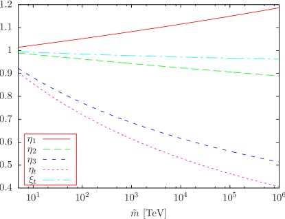
We show η1subscript𝜂1\eta_{1}, η2subscript𝜂2\eta_{2}, η3subscript𝜂3\eta_{3}, ηtsubscript𝜂𝑡\eta_{t} and ξtsubscript𝜉𝑡\xi_{t} as functions of m~~𝑚\tilde{m} with μ=|mg~|𝜇subscript𝑚~𝑔\mu=|m_{\tilde{g}}| in Fig. 2.

Refer to caption
Figure 2: Variables η1subscript𝜂1\eta_{1}, η2subscript𝜂2\eta_{2}, η3subscript𝜂3\eta_{3}, ηtsubscript𝜂𝑡\eta_{t} and ξtsubscript𝜉𝑡\xi_{t} in Eqs. (3034) as functions of m~~𝑚\tilde{m}, fixing μ=|mg~|𝜇subscript𝑚~𝑔\mu=|m_{\tilde{g}}|. We take mg~=1.5subscript𝑚~𝑔1.5m_{\tilde{g}}=1.5 TeV and mW~=200subscript𝑚~𝑊200m_{\tilde{W}}=200 GeV.

Here we set mg~=1.5subscript𝑚~𝑔1.5m_{\tilde{g}}=1.5 TeV, mW~=200subscript𝑚~𝑊200m_{\tilde{W}}=200 GeV and mB~=400subscript𝑚~𝐵400m_{\tilde{B}}=400 GeV.444 Very recently, a search of disappearing charged tracks by the ATLAS collaboration gives severe constraint on the mass of the Wino LSP. If the Higgsino mass is large enough and we adopt two-loop level mass splitting between W~±superscript~𝑊plus-or-minus\tilde{W}^{\pm} and W~0superscript~𝑊0\tilde{W}^{0} [35], we obtain mW~>270GeVsubscript𝑚~𝑊270GeVm_{\tilde{W}}>270~{}{\rm GeV} [36]. However, our analysis is almost independent on the Wino mass, then, we take this value as a reference point. By using these variables given in Eqs. (3038), the solution to the RG equations in Eqs. (1721) is written as,

CijW~(μ)subscriptsuperscript𝐶~𝑊𝑖𝑗𝜇\displaystyle C^{\tilde{W}}_{ij}(\mu) =\displaystyle= η39/10η218/11CijW~(m~),superscriptsubscript𝜂3910superscriptsubscript𝜂21811subscriptsuperscript𝐶~𝑊𝑖𝑗~𝑚\displaystyle\eta_{3}^{-9/10}\eta_{2}^{-18/11}~{}C^{\tilde{W}}_{ij}(\tilde{m}), (39)
C3iW~(μ)subscriptsuperscript𝐶~𝑊3𝑖𝜇\displaystyle C^{\tilde{W}}_{3i}(\mu) =\displaystyle= η39/10η218/11ξt1/2C3iW~(m~),superscriptsubscript𝜂3910superscriptsubscript𝜂21811superscriptsubscript𝜉𝑡12subscriptsuperscript𝐶~𝑊3𝑖~𝑚\displaystyle\eta_{3}^{-9/10}\eta_{2}^{-18/11}~{}\xi_{t}^{1/2}C^{\tilde{W}}_{3i}(\tilde{m}), (40)
C33W~(μ)subscriptsuperscript𝐶~𝑊33𝜇\displaystyle C^{\tilde{W}}_{33}(\mu) =\displaystyle= η39/10η218/11ξtC33W~(m~),superscriptsubscript𝜂3910superscriptsubscript𝜂21811subscript𝜉𝑡subscriptsuperscript𝐶~𝑊33~𝑚\displaystyle\eta_{3}^{-9/10}\eta_{2}^{-18/11}~{}\xi_{t}C^{\tilde{W}}_{33}(\tilde{m}), (41)
CQ,iiB~(μ)subscriptsuperscript𝐶~𝐵𝑄𝑖𝑖𝜇\displaystyle C^{\tilde{B}}_{Q,ii}(\mu) =\displaystyle= η39/10[CQ,iiB~(m~)+yC¯B~(m~)],superscriptsubscript𝜂3910delimited-[]subscriptsuperscript𝐶~𝐵𝑄𝑖𝑖~𝑚𝑦superscript¯𝐶~𝐵~𝑚\displaystyle\eta_{3}^{-9/10}~{}\left[C^{\tilde{B}}_{Q,ii}(\tilde{m})+y\bar{C}^{\tilde{B}}(\tilde{m})\right], (42)
CQ,12B~(μ)subscriptsuperscript𝐶~𝐵𝑄12𝜇\displaystyle C^{\tilde{B}}_{Q,12}(\mu) =\displaystyle= η39/10CQ,12B~(m~),superscriptsubscript𝜂3910subscriptsuperscript𝐶~𝐵𝑄12~𝑚\displaystyle\eta_{3}^{-9/10}~{}C^{\tilde{B}}_{Q,12}(\tilde{m}), (43)
CQ,33B~(μ)subscriptsuperscript𝐶~𝐵𝑄33𝜇\displaystyle C^{\tilde{B}}_{Q,33}(\mu) =\displaystyle= η39/10[(1+z)CQ,33B~(m~)zCu,33B~(m~)+yC¯B~(m~)],superscriptsubscript𝜂3910delimited-[]1𝑧subscriptsuperscript𝐶~𝐵𝑄33~𝑚𝑧subscriptsuperscript𝐶~𝐵𝑢33~𝑚𝑦superscript¯𝐶~𝐵~𝑚\displaystyle\eta_{3}^{-9/10}~{}\left[(1+z)C^{\tilde{B}}_{Q,33}(\tilde{m})-zC^{\tilde{B}}_{u,33}(\tilde{m})+y\bar{C}^{\tilde{B}}(\tilde{m})\right], (44)
CQ,3iB~(μ)subscriptsuperscript𝐶~𝐵𝑄3𝑖𝜇\displaystyle C^{\tilde{B}}_{Q,3i}(\mu) =\displaystyle= η39/10[(1+z)CQ,3iB~(m~)zCu,3iB~(m~)],superscriptsubscript𝜂3910delimited-[]1superscript𝑧subscriptsuperscript𝐶~𝐵𝑄3𝑖~𝑚superscript𝑧subscriptsuperscript𝐶~𝐵𝑢3𝑖~𝑚\displaystyle\eta_{3}^{-9/10}~{}\left[(1+z^{\prime})C^{\tilde{B}}_{Q,3i}(\tilde{m})-z^{\prime}C^{\tilde{B}}_{u,3i}(\tilde{m})\right], (45)
Cu,iiB~(μ)subscriptsuperscript𝐶~𝐵𝑢𝑖𝑖𝜇\displaystyle C^{\tilde{B}}_{u,ii}(\mu) =\displaystyle= η39/10[Cu,iiB~(m~)+yC¯B~(m~)],superscriptsubscript𝜂3910delimited-[]subscriptsuperscript𝐶~𝐵𝑢𝑖𝑖~𝑚𝑦superscript¯𝐶~𝐵~𝑚\displaystyle\eta_{3}^{-9/10}~{}\left[C^{\tilde{B}}_{u,ii}(\tilde{m})+y\bar{C}^{\tilde{B}}(\tilde{m})\right], (46)
Cu,12B~(μ)subscriptsuperscript𝐶~𝐵𝑢12𝜇\displaystyle C^{\tilde{B}}_{u,12}(\mu) =\displaystyle= η39/10Cu,12B~(m~),superscriptsubscript𝜂3910subscriptsuperscript𝐶~𝐵𝑢12~𝑚\displaystyle\eta_{3}^{-9/10}~{}C^{\tilde{B}}_{u,12}(\tilde{m}), (47)
Cu,33B~(μ)subscriptsuperscript𝐶~𝐵𝑢33𝜇\displaystyle C^{\tilde{B}}_{u,33}(\mu) =\displaystyle= η39/10[(1+2z)Cu,33B~(m~)2zCQ,33B~(m~)+yC¯B~(m~)],superscriptsubscript𝜂3910delimited-[]12𝑧subscriptsuperscript𝐶~𝐵𝑢33~𝑚2𝑧subscriptsuperscript𝐶~𝐵𝑄33~𝑚𝑦superscript¯𝐶~𝐵~𝑚\displaystyle\eta_{3}^{-9/10}~{}\left[(1+2z)C^{\tilde{B}}_{u,33}(\tilde{m})-2zC^{\tilde{B}}_{Q,33}(\tilde{m})+y\bar{C}^{\tilde{B}}(\tilde{m})\right], (48)
Cu,3iB~(μ)subscriptsuperscript𝐶~𝐵𝑢3𝑖𝜇\displaystyle C^{\tilde{B}}_{u,3i}(\mu) =\displaystyle= η39/10[(1+2z)Cu,3iB~(m~)2zCQ,3iB~(m~)],superscriptsubscript𝜂3910delimited-[]12superscript𝑧subscriptsuperscript𝐶~𝐵𝑢3𝑖~𝑚2superscript𝑧subscriptsuperscript𝐶~𝐵𝑄3𝑖~𝑚\displaystyle\eta_{3}^{-9/10}~{}\left[(1+2z^{\prime})C^{\tilde{B}}_{u,3i}(\tilde{m})-2z^{\prime}C^{\tilde{B}}_{Q,3i}(\tilde{m})\right], (49)
Cd,iiB~(μ)subscriptsuperscript𝐶~𝐵𝑑𝑖𝑖𝜇\displaystyle C^{\tilde{B}}_{d,ii}(\mu) =\displaystyle= η39/10[Cd,iiB~(m~)+yC¯B~(m~)],superscriptsubscript𝜂3910delimited-[]subscriptsuperscript𝐶~𝐵𝑑𝑖𝑖~𝑚𝑦superscript¯𝐶~𝐵~𝑚\displaystyle\eta_{3}^{-9/10}~{}\left[C^{\tilde{B}}_{d,ii}(\tilde{m})+y\bar{C}^{\tilde{B}}(\tilde{m})\right], (50)
Cd,12B~(μ)subscriptsuperscript𝐶~𝐵𝑑12𝜇\displaystyle C^{\tilde{B}}_{d,12}(\mu) =\displaystyle= η39/10Cd,12B~(m~),superscriptsubscript𝜂3910subscriptsuperscript𝐶~𝐵𝑑12~𝑚\displaystyle\eta_{3}^{-9/10}~{}C^{\tilde{B}}_{d,12}(\tilde{m}), (51)
Cd,33B~(μ)subscriptsuperscript𝐶~𝐵𝑑33𝜇\displaystyle C^{\tilde{B}}_{d,33}(\mu) =\displaystyle= η39/10[Cd,33B~(m~)+yC¯B~(m~)],superscriptsubscript𝜂3910delimited-[]subscriptsuperscript𝐶~𝐵𝑑33~𝑚𝑦superscript¯𝐶~𝐵~𝑚\displaystyle\eta_{3}^{-9/10}~{}\left[C^{\tilde{B}}_{d,33}(\tilde{m})+y\bar{C}^{\tilde{B}}(\tilde{m})\right], (52)
Cd,3iB~(μ)subscriptsuperscript𝐶~𝐵𝑑3𝑖𝜇\displaystyle C^{\tilde{B}}_{d,3i}(\mu) =\displaystyle= η39/10Cd,3iB~(m~),superscriptsubscript𝜂3910subscriptsuperscript𝐶~𝐵𝑑3𝑖~𝑚\displaystyle\eta_{3}^{-9/10}~{}C^{\tilde{B}}_{d,3i}(\tilde{m}), (53)
C7B~(μ)subscriptsuperscript𝐶~𝐵7𝜇\displaystyle C^{\tilde{B}}_{7}(\mu) =\displaystyle= η37/5C7B~(m~).superscriptsubscript𝜂375subscriptsuperscript𝐶~𝐵7~𝑚\displaystyle\eta_{3}^{-7/5}~{}C^{\tilde{B}}_{7}(\tilde{m}). (54)

Here, i𝑖i runs a light flavor index 1,2121,2. Note that we have dropped off-diagonal elements of Yukawa matrices. Then, off-diagonal elements of C𝐶C’s are valid only if the contribution of off-diagonal elements of Yukawa is much smaller than them. For example, C12W~(μ)subscriptsuperscript𝐶~𝑊12𝜇C^{\tilde{W}}_{12}(\mu) in Eq. (39) is valid only if C12W~(m~)subscriptsuperscript𝐶~𝑊12~𝑚C^{\tilde{W}}_{12}(\tilde{m}) is much larger than Yu,12Yu,22C22W~(m~)subscript𝑌𝑢12subscript𝑌𝑢22subscriptsuperscript𝐶~𝑊22~𝑚Y_{u,12}Y_{u,22}C^{\tilde{W}}_{22}(\tilde{m}) and Yu,13Yu,23C33W~(m~)subscript𝑌𝑢13subscript𝑌𝑢23subscriptsuperscript𝐶~𝑊33~𝑚Y_{u,13}Y_{u,23}C^{\tilde{W}}_{33}(\tilde{m}).

2.3 Numerical Analysis of Gluino decay

So far, we discussed leading logarithm corrections for the Wilson coefficients relevant to the gluino decay. To extract information on the squark sector from the gluino decay, it is important to take into account such corrections. In this subsection, we discuss the effects of leading logarithm corrections on the lifetime and decay pattern of the gluino numerically. In the present situation, gluino two-body decay (g~gB~~𝑔𝑔~𝐵\tilde{g}\to g\tilde{B}) can be neglected because of one-loop suppression.555 If the Higgsino is lighter than the gluino, the decay width of this two body decay mode is enhanced because of large logarithmic corrections [30, 31, 32]. Then, this mode can be significant. In the limit that |mg~||mW~|,|mg~||mB~|mtmuch-greater-thansubscript𝑚~𝑔subscript𝑚~𝑊subscript𝑚~𝑔subscript𝑚~𝐵subscript𝑚𝑡|m_{\tilde{g}}|-|m_{\tilde{W}}|,~{}|m_{\tilde{g}}|-|m_{\tilde{B}}|\gg m_{t} and VCKM𝟏similar-to-or-equalssubscript𝑉CKM1V_{\rm CKM}\simeq{\bf 1}, we can approximately get the following analytical formulae [31, 37]:

Γ(g~B~uLiu¯Lj)=Γ(g~B~dLid¯Lj)Γ~𝑔~𝐵subscript𝑢𝐿𝑖subscript¯𝑢𝐿𝑗Γ~𝑔~𝐵subscript𝑑𝐿𝑖subscript¯𝑑𝐿𝑗\displaystyle\Gamma(\tilde{g}\to\tilde{B}u_{Li}\bar{u}_{Lj})=\Gamma(\tilde{g}\to\tilde{B}d_{Li}\bar{d}_{Lj}) =|CQ,ijB~|2|mg~|51536π3m~4f(mB~/mg~),absentsuperscriptsuperscriptsubscript𝐶𝑄𝑖𝑗~𝐵2superscriptsubscript𝑚~𝑔51536superscript𝜋3superscript~𝑚4𝑓subscript𝑚~𝐵subscript𝑚~𝑔\displaystyle=\frac{|C_{Q,ij}^{\tilde{B}}|^{2}|m_{\tilde{g}}|^{5}}{1536\pi^{3}{\tilde{m}}^{4}}f\left(m_{\tilde{B}}/m_{\tilde{g}}\right), (55)
Γ(g~B~uRiu¯Rj)Γ~𝑔~𝐵subscript𝑢𝑅𝑖subscript¯𝑢𝑅𝑗\displaystyle\Gamma(\tilde{g}\to\tilde{B}u_{Ri}\bar{u}_{Rj}) =|Cu,ijB~|2|mg~|51536π3m~4f(mB~/mg~),absentsuperscriptsuperscriptsubscript𝐶𝑢𝑖𝑗~𝐵2superscriptsubscript𝑚~𝑔51536superscript𝜋3superscript~𝑚4𝑓subscript𝑚~𝐵subscript𝑚~𝑔\displaystyle=\frac{|C_{u,ij}^{\tilde{B}}|^{2}|m_{\tilde{g}}|^{5}}{1536\pi^{3}{\tilde{m}}^{4}}f\left(m_{\tilde{B}}/m_{\tilde{g}}\right), (56)
Γ(g~B~dRid¯Rj)Γ~𝑔~𝐵subscript𝑑𝑅𝑖subscript¯𝑑𝑅𝑗\displaystyle\Gamma(\tilde{g}\to\tilde{B}d_{Ri}\bar{d}_{Rj}) =|Cd,ijB~|2|mg~|51536π3m~4f(mB~/mg~),absentsuperscriptsuperscriptsubscript𝐶𝑑𝑖𝑗~𝐵2superscriptsubscript𝑚~𝑔51536superscript𝜋3superscript~𝑚4𝑓subscript𝑚~𝐵subscript𝑚~𝑔\displaystyle=\frac{|C_{d,ij}^{\tilde{B}}|^{2}|m_{\tilde{g}}|^{5}}{1536\pi^{3}{\tilde{m}}^{4}}f\left(m_{\tilde{B}}/m_{\tilde{g}}\right), (57)
Γ(g~W~0uLiu¯Lj)=Γ(g~W~0dLid¯Lj)Γ~𝑔superscript~𝑊0subscript𝑢𝐿𝑖subscript¯𝑢𝐿𝑗Γ~𝑔superscript~𝑊0subscript𝑑𝐿𝑖subscript¯𝑑𝐿𝑗\displaystyle\Gamma(\tilde{g}\to\tilde{W}^{0}u_{Li}\bar{u}_{Lj})=\Gamma(\tilde{g}\to\tilde{W}^{0}d_{Li}\bar{d}_{Lj}) =|CijW~|2|mg~|51536π3m~4f(mW~/mg~),absentsuperscriptsuperscriptsubscript𝐶𝑖𝑗~𝑊2superscriptsubscript𝑚~𝑔51536superscript𝜋3superscript~𝑚4𝑓subscript𝑚~𝑊subscript𝑚~𝑔\displaystyle=\frac{|C_{ij}^{\tilde{W}}|^{2}|m_{\tilde{g}}|^{5}}{1536\pi^{3}{\tilde{m}}^{4}}f\left(m_{\tilde{W}}/m_{\tilde{g}}\right), (58)
Γ(g~W~+dLiu¯Lj)=Γ(g~W~uLid¯Lj)Γ~𝑔superscript~𝑊subscript𝑑𝐿𝑖subscript¯𝑢𝐿𝑗Γ~𝑔superscript~𝑊subscript𝑢𝐿𝑖subscript¯𝑑𝐿𝑗\displaystyle\Gamma(\tilde{g}\to\tilde{W}^{+}d_{Li}\bar{u}_{Lj})=\Gamma(\tilde{g}\to\tilde{W}^{-}u_{Li}\bar{d}_{Lj}) =2|CijW~|2|mg~|51536π3m~4f(mW~/mg~).absent2superscriptsubscriptsuperscript𝐶~𝑊𝑖𝑗2superscriptsubscript𝑚~𝑔51536superscript𝜋3superscript~𝑚4𝑓subscript𝑚~𝑊subscript𝑚~𝑔\displaystyle=\frac{2|C^{\tilde{W}}_{ij}|^{2}|m_{\tilde{g}}|^{5}}{1536\pi^{3}{\tilde{m}}^{4}}f\left(m_{\tilde{W}}/m_{\tilde{g}}\right). (59)

Here, f(x)=18|x|212|x|4log|x|2+8|x|6|x|8+2(1+9|x|2+6|x|4log|x|29|x|4+6|x|4log|x|2|x|6)Re(x)𝑓𝑥18superscript𝑥212superscript𝑥4superscript𝑥28superscript𝑥6superscript𝑥8219superscript𝑥26superscript𝑥4superscript𝑥29superscript𝑥46superscript𝑥4superscript𝑥2superscript𝑥6Re𝑥f(x)=1-8|x|^{2}-12|x|^{4}\log|x|^{2}+8|x|^{6}-|x|^{8}+2(1+9|x|^{2}+6|x|^{4}\log|x|^{2}-9|x|^{4}+6|x|^{4}\log|x|^{2}-|x|^{6}){\rm Re}(x). As for operators whose dimension is higher than six, we use tree-level amplitudes in our numerical calculation. In the following of this section, we denote decay widths calculated by C(μ=m~)𝐶𝜇~𝑚C(\mu=\tilde{m}) and C(μ=|mg~|)𝐶𝜇subscript𝑚~𝑔C(\mu=|m_{\tilde{g}}|) as “tree” and “resum”, respectively.

Total decay width

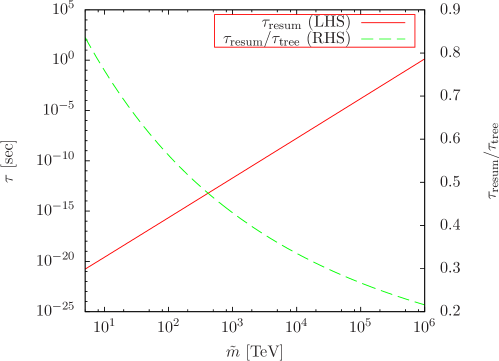
It is pointed out that the lifetime of the gluino is significantly affected by the resummation of leading logarithmic corrections [31]. We show the lifetime of the gluino in Fig. 3. Here we take mQ~L2=mu~R2=md~R2=m~2×𝟙superscriptsubscript𝑚subscript~𝑄𝐿2superscriptsubscript𝑚subscript~𝑢𝑅2superscriptsubscript𝑚subscript~𝑑𝑅2superscript~𝑚21m_{\tilde{Q}_{L}}^{2}=m_{\tilde{u}_{R}}^{2}=m_{\tilde{d}_{R}}^{2}=\tilde{m}^{2}\times{\mathbb{1}}. We can see that the quantum corrections make the decay rate double for m~=103~𝑚superscript103\tilde{m}=10^{3} TeV.

Refer to caption
Figure 3: The red and solid line shows the lifetime of the gluino with resummation. The green and dashed line shows the ratio of the resummed lifetime to tree-level one. We take the gaugino masses as mW~=200GeVsubscript𝑚~𝑊200GeVm_{\tilde{W}}=200~{}{\rm GeV}, mB~=400GeVsubscript𝑚~𝐵400GeVm_{\tilde{B}}=400~{}{\rm GeV} and mg~=1.5TeVsubscript𝑚~𝑔1.5TeVm_{\tilde{g}}=-1.5~{}{\rm TeV}. For the squark mass, we take universal squark masses at the squark mass scale.

Branching fraction of g~W~qq¯~𝑔~𝑊𝑞¯𝑞\tilde{g}\to\tilde{W}q\bar{q} and g~B~qq¯~𝑔~𝐵𝑞¯𝑞\tilde{g}\to\tilde{B}q\bar{q}

In the case of the heavy Higgsino, the low-mass neutralinos and charginos are almost pure Wino or Bino states. Therefore discriminating the gluino decay mode into a Wino and Bino can be experimentally viable. This branching ratio reveals the relation between left-handed squarks and right-handed ones. Thus, precise estimation of the branching ratio is significant.

At tree level, the Wilson coefficients of the operators involving W~~𝑊\tilde{W} are proportional to the gauge coupling g𝑔g, and those involving B~~𝐵\tilde{B} are proportional to gsuperscript𝑔g^{\prime}. They are proportional to αsuperscript𝛼\alpha^{\prime} and α𝛼\alpha at tree level, however, leading log resummation alters ratio between them.

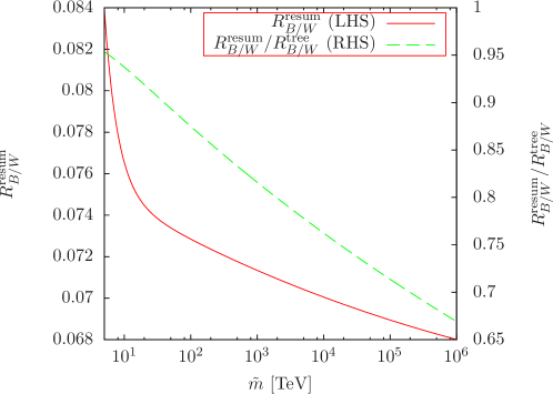
In Fig. 4, we plot RB~/W~subscript𝑅~𝐵~𝑊R_{\tilde{B}/\tilde{W}} as a function of squark masses, which is defined as,

RB~/W~subscript𝑅~𝐵~𝑊\displaystyle R_{\tilde{B}/\tilde{W}} \displaystyle\equiv qΓ(g~B~qq¯)qΓ(g~W~qq¯).subscript𝑞Γ~𝑔~𝐵𝑞¯𝑞subscript𝑞Γ~𝑔~𝑊𝑞¯𝑞\displaystyle\frac{\sum_{q}\Gamma(\tilde{g}\to\tilde{B}q\bar{q})}{\sum_{q}\Gamma(\tilde{g}\to\tilde{W}q\bar{q})}. (60)

Here we take mQ~L2=mu~R2=md~R2=m~2×𝟙superscriptsubscript𝑚subscript~𝑄𝐿2superscriptsubscript𝑚subscript~𝑢𝑅2superscriptsubscript𝑚subscript~𝑑𝑅2superscript~𝑚21m_{\tilde{Q}_{L}}^{2}=m_{\tilde{u}_{R}}^{2}=m_{\tilde{d}_{R}}^{2}=\tilde{m}^{2}\times{\mathbb{1}}. We can see that resummation of leading logarithm corrections alters branching fractions by about 20 % for m~=103~𝑚superscript103\tilde{m}=10^{3} TeV.

Refer to caption
Figure 4: RB~/W~|resumevaluated-atsubscript𝑅~𝐵~𝑊resumR_{\tilde{B}/\tilde{W}}|_{\rm resum} (red and solid line) and the ratio of the resummed one to tree-level one (green and dashed line). We take the gaugino masses as mW~=200GeVsubscript𝑚~𝑊200GeVm_{\tilde{W}}=200~{}{\rm GeV}, mB~=400GeVsubscript𝑚~𝐵400GeVm_{\tilde{B}}=400~{}{\rm GeV} and mg~=1.5TeVsubscript𝑚~𝑔1.5TeVm_{\tilde{g}}=-1.5~{}{\rm TeV}. For the squark mass, we take universal squark mass at for m~=103~𝑚superscript103\tilde{m}=10^{3} TeV.quark mass scale.

Flavor structure of g~W~qq¯~𝑔~𝑊𝑞¯𝑞\tilde{g}\to\tilde{W}q\bar{q}

The flavor structure of g~W~qq¯~𝑔~𝑊𝑞¯𝑞\tilde{g}\to\tilde{W}q\bar{q} is determined by (mQ~L2)1superscriptsubscriptsuperscript𝑚2subscript~𝑄𝐿1(m^{2}_{\tilde{Q}_{L}})^{-1} at tree level, and it suffers from leading logarithm corrections because of the anomalous dimension of the quarks. An important source of the corrections is top Yukawa ytsubscript𝑦𝑡y_{t}. It changes g~W~0tt¯~𝑔superscript~𝑊0𝑡¯𝑡\tilde{g}\to\tilde{W}^{0}t\bar{t} relative ratio to g~W~qq¯~𝑔~𝑊𝑞¯𝑞\tilde{g}\to\tilde{W}q\bar{q}.

Rtt/qqW~subscriptsuperscript𝑅~𝑊𝑡𝑡𝑞𝑞\displaystyle R^{\tilde{W}}_{tt/qq} \displaystyle\equiv Γ(g~W~0tt¯)Γ(g~W~qiq¯j),Γ~𝑔superscript~𝑊0𝑡¯𝑡Γ~𝑔~𝑊subscript𝑞𝑖subscript¯𝑞𝑗\displaystyle\frac{\Gamma(\tilde{g}\to\tilde{W}^{0}t\bar{t})}{\Gamma(\tilde{g}\to\tilde{W}q_{i}\bar{q}_{j})}, (61)

where i,j=1,2formulae-sequence𝑖𝑗12i,j=1,2. The ratio of resummed result to tree-level one is (Rtt/qqW~|resum)/(Rtt/qqW~|tree)=ξt2evaluated-atsubscriptsuperscript𝑅~𝑊𝑡𝑡𝑞𝑞resumevaluated-atsubscriptsuperscript𝑅~𝑊𝑡𝑡𝑞𝑞treesuperscriptsubscript𝜉𝑡2(R^{\tilde{W}}_{tt/qq}|_{\rm resum})/(R^{\tilde{W}}_{tt/qq}|_{\rm tree})=\xi_{t}^{2}. As seen in Fig. 2, Rtt/qqW~subscriptsuperscript𝑅~𝑊𝑡𝑡𝑞𝑞R^{\tilde{W}}_{tt/qq} is decreased by the effect of resummation of leading logarithm correction by 3–4 %, compared to the tree-level result.

Flavor structure of g~B~qq¯~𝑔~𝐵𝑞¯𝑞\tilde{g}\to\tilde{B}q\bar{q}

Here, we discuss radiative correction for the following quantities:

Rtc/ttB~=Γ(g~B~tc¯/B~t¯c)Γ(g~B~tt¯),Rtc/ccB~=Γ(g~B~tc¯/B~t¯c)Γ(g~B~cc¯).formulae-sequencesubscriptsuperscript𝑅~𝐵𝑡𝑐𝑡𝑡Γ~𝑔~𝐵𝑡¯𝑐~𝐵¯𝑡𝑐Γ~𝑔~𝐵𝑡¯𝑡subscriptsuperscript𝑅~𝐵𝑡𝑐𝑐𝑐Γ~𝑔~𝐵𝑡¯𝑐~𝐵¯𝑡𝑐Γ~𝑔~𝐵𝑐¯𝑐\displaystyle R^{\tilde{B}}_{tc/tt}~{}=~{}\frac{\Gamma(\tilde{g}\to\tilde{B}t\bar{c}/\tilde{B}\bar{t}c)}{\Gamma(\tilde{g}\to\tilde{B}t\bar{t})},\quad\quad\quad R^{\tilde{B}}_{tc/cc}~{}=~{}\frac{\Gamma(\tilde{g}\to\tilde{B}t\bar{c}/\tilde{B}\bar{t}c)}{\Gamma(\tilde{g}\to\tilde{B}c\bar{c})}. (62)

Compared to the Wino case, radiative corrections for the decay into the Bino more significantly affect the flavor structure of the gluino decay. This is because the contribution of the top Yukawa coupling is larger. In addition, the penguin-like diagram contribution in Fig. 1 affects only the flavor diagonal part. Thus, the RG evolution of the Wilson coefficients has different feature between the flavor conserving and violating parts. We show numerical results in the following two sample cases.

  • Refer to caption
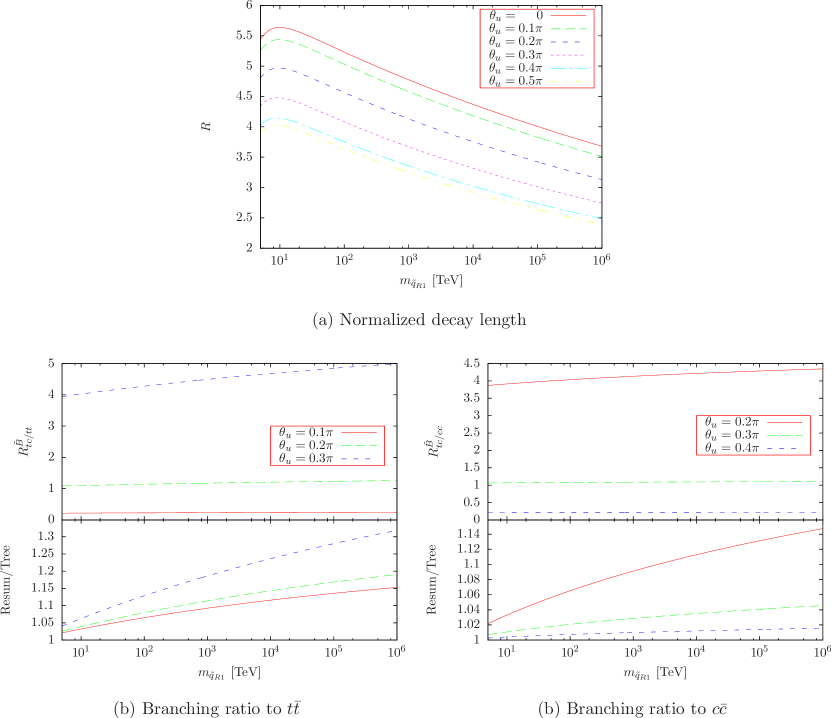
    Figure 5: Normalized decay length which is defined as R=(cτg~/1cm)(m0/1000TeV)4𝑅𝑐subscript𝜏~𝑔1cmsuperscriptsubscript𝑚01000TeV4R=(c\tau_{\tilde{g}}/1~{}{\rm cm})(m_{0}/1000~{}{\rm TeV})^{4} (a), branching ratio Rtc/ttB~subscriptsuperscript𝑅~𝐵𝑡𝑐𝑡𝑡R^{\tilde{B}}_{tc/tt} (b) and Rtc/ccB~subscriptsuperscript𝑅~𝐵𝑡𝑐𝑐𝑐R^{\tilde{B}}_{tc/cc} (c) in a case of light u~Rsubscript~𝑢𝑅\tilde{u}_{R}. We take the gaugino masses as mW~=200GeVsubscript𝑚~𝑊200GeVm_{\tilde{W}}=200~{}{\rm GeV}, mB~=400GeVsubscript𝑚~𝐵400GeVm_{\tilde{B}}=400~{}{\rm GeV} and mg~=1.5TeVsubscript𝑚~𝑔1.5TeVm_{\tilde{g}}=-1.5~{}{\rm TeV}.
  • light u~Rsubscript~𝑢𝑅\tilde{u}_{R}
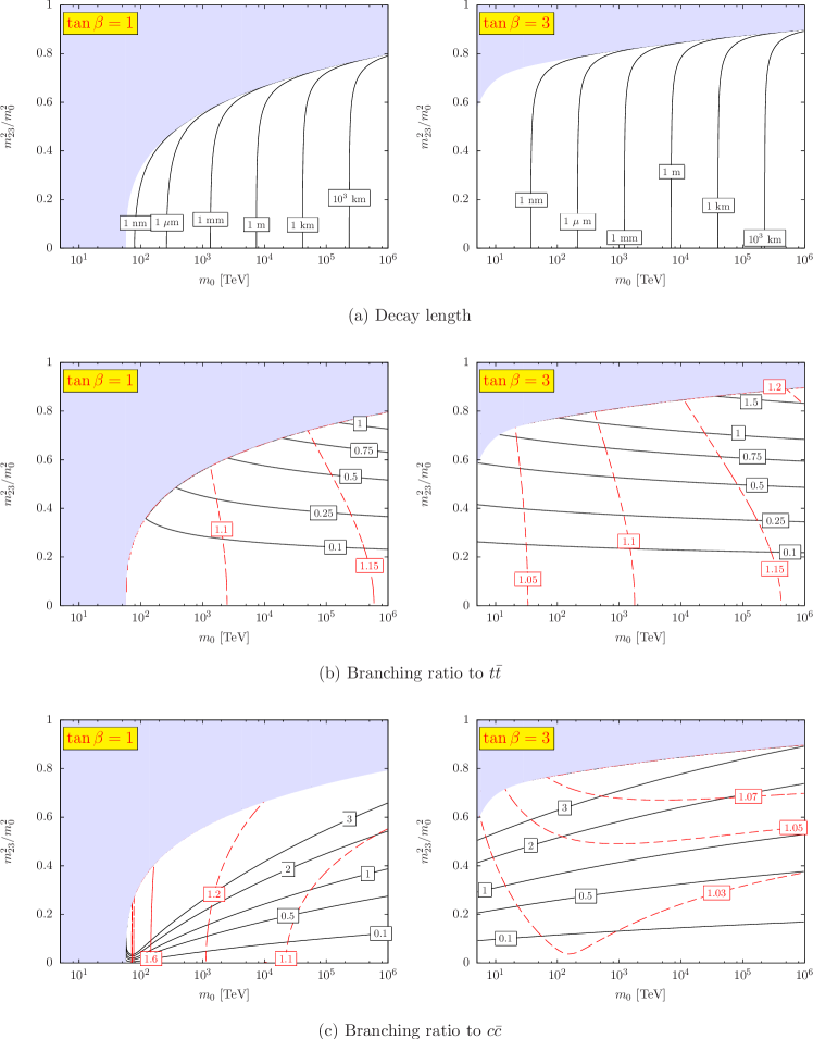
    In this case, we assume that the lightest squark q~R1subscript~𝑞𝑅1\tilde{q}_{R1} is a mixture of t~Rsubscript~𝑡𝑅\tilde{t}_{R} and c~Rsubscript~𝑐𝑅\tilde{c}_{R}, and other squarks are much heavier than them. The mixing angle θusubscript𝜃𝑢\theta_{u} is defined as q~R1=cosθut~R+sinθuc~Rsubscript~𝑞𝑅1subscript𝜃𝑢subscript~𝑡𝑅subscript𝜃𝑢subscript~𝑐𝑅\tilde{q}_{R1}=\cos\theta_{u}\tilde{t}_{R}+\sin\theta_{u}\tilde{c}_{R}. Fig. 5 shows the numerical result of the gluino decay length, Rtc/ttB~subscriptsuperscript𝑅~𝐵𝑡𝑐𝑡𝑡R^{\tilde{B}}_{tc/tt} and Rtc/ccB~subscriptsuperscript𝑅~𝐵𝑡𝑐𝑐𝑐R^{\tilde{B}}_{tc/cc}. Here we define a normalization variable R𝑅R for the gluino decay length as

    cτg~=R×1cm(mq~R11000TeV)4.𝑐subscript𝜏~𝑔𝑅1cmsuperscriptsubscript𝑚subscript~𝑞𝑅11000TeV4\displaystyle c\tau_{\tilde{g}}=R\times 1~{}{\rm cm}\left(\frac{m_{\tilde{q}_{R1}}}{1000~{}{\rm TeV}}\right)^{4}. (63)

    We can see Rtc/ttB~|resumevaluated-atsubscriptsuperscript𝑅~𝐵𝑡𝑐𝑡𝑡resumR^{\tilde{B}}_{tc/tt}|_{\rm resum} (Rtc/ccB~|resumevaluated-atsubscriptsuperscript𝑅~𝐵𝑡𝑐𝑐𝑐resumR^{\tilde{B}}_{tc/cc}|_{\rm resum}) is enhanced compared to Rtc/ttB~|treeevaluated-atsubscriptsuperscript𝑅~𝐵𝑡𝑐𝑡𝑡treeR^{\tilde{B}}_{tc/tt}|_{\rm tree} (Rtc/ccB~|treeevaluated-atsubscriptsuperscript𝑅~𝐵𝑡𝑐𝑐𝑐treeR^{\tilde{B}}_{tc/cc}|_{\rm tree}) results by 10–20 %.

  • mSUGRA-like case
    In this case, at the “GUT” scale μ=2×10¹⁶𝜇2superscript1016\mu=2\times 10^{16} GeV, we take the diagonal elements of the squark mass-squared as mQ~L,ii2=mu~R,ii2=md~R,ii2=m02superscriptsubscript𝑚subscript~𝑄𝐿𝑖𝑖2superscriptsubscript𝑚subscript~𝑢𝑅𝑖𝑖2superscriptsubscript𝑚subscript~𝑑𝑅𝑖𝑖2superscriptsubscript𝑚02m_{\tilde{Q}_{L},ii}^{2}=m_{\tilde{u}_{R},ii}^{2}=m_{\tilde{d}_{R},ii}^{2}=m_{0}^{2} (i=1,2,3𝑖123i=1,2,3), the off-diagonal elements as mu~R,232=mu~R,322=m232superscriptsubscript𝑚subscript~𝑢𝑅232superscriptsubscript𝑚subscript~𝑢𝑅322superscriptsubscript𝑚232m_{\tilde{u}_{R},23}^{2}=m_{\tilde{u}_{R},32}^{2}=m_{23}^{2} and the other components to be zero. For other parameters, we take mW~=200GeV,mB~=400GeV,mg~=1.5TeVformulae-sequencesubscript𝑚~𝑊200GeVformulae-sequencesubscript𝑚~𝐵400GeVsubscript𝑚~𝑔1.5TeVm_{\tilde{W}}=200~{}{\rm GeV},~{}m_{\tilde{B}}=400~{}{\rm GeV},~{}m_{\tilde{g}}=-1.5~{}{\rm TeV} and tanβ=1,3𝛽13\tan\beta=1,3. By using RG equations for the squark soft parameters, we obtain physical squark masses and mixings. In calculation of soft mass RG evolution, we neglect terms other than top Yukawa parts. We also assume b𝑏b, μ𝜇\mu and mHd2superscriptsubscript𝑚subscript𝐻𝑑2m_{H_{d}}^{2} are optimized so that the correct electroweak breaking occurs.

    For estimation of the gluino decay width, we take the matching scale m~~𝑚\tilde{m} as the lightest squark mass. In this case, the RG effect from the top Yukawa coupling decreases mt~Rsubscript𝑚subscript~𝑡𝑅m_{\tilde{t}_{R}} and the decay into tt¯B~𝑡¯𝑡~𝐵t\bar{t}\tilde{B} is enhanced. Fig. 6 shows the numerical result of Rtc/ttB~subscriptsuperscript𝑅~𝐵𝑡𝑐𝑡𝑡R^{\tilde{B}}_{tc/tt}. The shaded region shows the region where the lightest squark is lighter than the gluino or a tachyon. We can see Rtc/ttB~|resumevaluated-atsubscriptsuperscript𝑅~𝐵𝑡𝑐𝑡𝑡resumR^{\tilde{B}}_{tc/tt}|_{\rm resum} (Rtc/ccB~|resumevaluated-atsubscriptsuperscript𝑅~𝐵𝑡𝑐𝑐𝑐resumR^{\tilde{B}}_{tc/cc}|_{\rm resum}) is enhanced compared to Rtc/ttB~|treeevaluated-atsubscriptsuperscript𝑅~𝐵𝑡𝑐𝑡𝑡treeR^{\tilde{B}}_{tc/tt}|_{\rm tree} (Rtc/ccB~|treeevaluated-atsubscriptsuperscript𝑅~𝐵𝑡𝑐𝑐𝑐treeR^{\tilde{B}}_{tc/cc}|_{\rm tree}) results by about 10 % for m0=𝒪(103)subscript𝑚0𝒪superscript103m_{0}={\cal O}(10^{3}) TeV.

    Refer to caption
    Figure 6: Decay length cτg~𝑐subscript𝜏~𝑔c\tau_{\tilde{g}} (a), Branching fraction Rtc/ttB~subscriptsuperscript𝑅~𝐵𝑡𝑐𝑡𝑡R^{\tilde{B}}_{tc/tt} (b) and Rtc/ccB~subscriptsuperscript𝑅~𝐵𝑡𝑐𝑐𝑐R^{\tilde{B}}_{tc/cc} (c) in mSUGRA-like case. In shaded region of the above figures, the lightest squark becomes lighter than the gluino or a tachyon. In figures (b) and (c), black lines show branching ratio Rtc/ttB~subscriptsuperscript𝑅~𝐵𝑡𝑐𝑡𝑡R^{\tilde{B}}_{tc/tt} and Rtc/ccB~subscriptsuperscript𝑅~𝐵𝑡𝑐𝑐𝑐R^{\tilde{B}}_{tc/cc}, respectively, and red-dashed lines shows each Rresum/Rtreesubscript𝑅resumsubscript𝑅treeR_{\rm resum}/R_{\rm tree}.

3 Low-energy Flavor Constraints and Gluino Decay

As we have discussed above, the gluino decay directly reflects the structure of the squark sector. For example, the flavor violation of the squark sector leads the flavor violating gluino decay, such as g~tcχ~~𝑔𝑡𝑐~𝜒\tilde{g}\to tc\tilde{\chi}. However, in general, the gluino-squark interactions which control the gluino decay, also contribute to low-energy rare processes such as meson mixings and electric dipole moments (EDM’s). Therefore, observations of the low-energy physics give constraints on the gluino decay process. In this section, we study the correlation between the low-energy flavor/CP observation and the gluino decay.

3.1 Flavor/CP Constraints

In general, SSMs can give visible contributions to low-energy flavor/CP violating processes, even if the SUSY breaking scale is high, say, higher than 𝒪(10)𝒪10{\cal O}(10) TeV. Here we discuss some low-energy observables, which can give strong constraints on the high-scale SUSY models. For reviews, see, e.g., Refs. [38, 39].

Here we adopt the super-CKM basis (see Appendix A for the correspondence to the weak-basis). We consider the following squark mass-squared matrices in this basis:

ma2=m02(1+Δ1aδ12aδ13aδ12a1+Δ2aδ23aδ13aδ231+Δ3a),subscriptsuperscript𝑚2𝑎superscriptsubscript𝑚02matrix1superscriptsubscriptΔ1𝑎superscriptsubscript𝛿12𝑎superscriptsubscript𝛿13𝑎superscriptsubscript𝛿12𝑎1superscriptsubscriptΔ2𝑎superscriptsubscript𝛿23𝑎superscriptsubscript𝛿13𝑎superscriptsubscript𝛿231superscriptsubscriptΔ3𝑎{m}^{2}_{a}\!=\!{m}_{0}^{2}\left(\begin{matrix}1+\Delta_{1}^{a}&\delta_{12}^{a}&\delta_{13}^{a}\\ \delta_{12}^{a*}&1+\Delta_{2}^{a}&\delta_{23}^{a}\\ \delta_{13}^{a*}&\delta_{23}^{*}&1+\Delta_{3}^{a}\\ \end{matrix}\right), (64)

where a=Q~L(d~L),u~R,d~R𝑎subscript~𝑄𝐿subscript~𝑑𝐿subscript~𝑢𝑅subscript~𝑑𝑅a=\tilde{Q}_{L}(\tilde{d}_{L}),\tilde{u}_{R},\tilde{d}_{R}. The mass-squared matrix for u~Lsubscript~𝑢𝐿\tilde{u}_{L} is obtained by m^u~L2=VCKMmQ~L2VCKMsubscriptsuperscript^𝑚2subscript~𝑢𝐿subscript𝑉CKMsubscriptsuperscript𝑚2subscript~𝑄𝐿superscriptsubscript𝑉CKM\hat{m}^{2}_{\tilde{u}_{L}}=V_{\rm CKM}\ {m}^{2}_{\tilde{Q}_{L}}V_{\rm CKM}^{\dagger}. For the assumption of some charge of the SUSY breaking field, we expect the sizes of A𝐴A-terms are order of the gaugino masses and neglect them. We discuss the current constraints on the flavor violating mass terms.

ΔF=2Δ𝐹2\Delta F=2 process

Refer to caption
Figure 7: Examples of diagrams relevant to low-energy constraints.

One of the strongest constraints on δ𝛿\delta’s comes from ΔF=2Δ𝐹2\Delta F=2 meson mixings. Squarks contribute to the low-energy ΔF=2Δ𝐹2\Delta F=2 operators via loop processes (Fig. 7-(a)). We consider only gluino mediated box diagrams, which give leading contributions. The K0K¯0superscript𝐾0superscript¯𝐾0K^{0}-\bar{K}^{0} system is well measured and gives the strongest constraint on the first and second generation flavor violation. This can constrain δ12Q~Lsuperscriptsubscript𝛿12subscript~𝑄𝐿\delta_{12}^{\tilde{Q}_{L}} and δ12d~Rsuperscriptsubscript𝛿12subscript~𝑑𝑅\delta_{12}^{\tilde{d}_{R}}, since they induce direct sd𝑠𝑑s-d mixings. Especially, simultaneous existences of δ12Q~Lsuperscriptsubscript𝛿12subscript~𝑄𝐿\delta_{12}^{\tilde{Q}_{L}}, δ12d~Rsuperscriptsubscript𝛿12subscript~𝑑𝑅\delta_{12}^{\tilde{d}_{R}} and CP-phase are drastically constrained. In addition, it can also constrain products of δ13subscript𝛿13\delta_{13} and δ23subscript𝛿23\delta_{23}. This is because a squark transition (132)132(1\to 3\to 2) induces large sd𝑠𝑑s-d transition.

ΔF=1Δ𝐹1\Delta F=1 process

The operators with ΔF=1Δ𝐹1\Delta F=1 induce ΔF=1Δ𝐹1\Delta F=1 heavy quark decays, such as bsγ𝑏𝑠𝛾b\to s\gamma. These operators are chirality-flipping, and thus the amplitudes of these processes depend on the size of μ𝜇\mu term. If the absolute value of μ𝜇\mu is as much as the squark scale, the observation from bsγ𝑏𝑠𝛾b\to s\gamma provides a strong constraint on the entry of 3-2 element of the squark mass-squared matrices. In the case of 𝒪(1)𝒪1{\cal O}(1) of δ23superscript𝛿23\delta^{23}, m0<𝒪(10)subscript𝑚0𝒪10m_{0}<{\cal O}(10) TeV is excluded.

ΔF=0Δ𝐹0\Delta F=0 process

Electric and chromo-electric dipole moments (EDM’s and CEDM’s) of quarks give constraints on the sfermion sector. Although the EDM and CEDM are not flavor violating processes, it can severely constrain the squark flavor violating structure, if both left and right-handed squarks sector have flavor/CP violations and the size of μ𝜇\mu is large. These operators are chirality-flipping and the coefficients are suppressed by the SM fermion masses. When the squark mass-squared matrix is flavor diagonal, these amplitudes are suppressed by the light quark mass (musubscript𝑚𝑢m_{u}, mdsubscript𝑚𝑑m_{d} and mssubscript𝑚𝑠m_{s}). However once one allows large flavor violation in the squark sector, the suppression is replaced with heavy quarks (mtsubscript𝑚𝑡m_{t} and mbsubscript𝑚𝑏m_{b}) and the size of EDM enhanced by mt,b/mu,d,ssubscript𝑚𝑡𝑏subscript𝑚𝑢𝑑𝑠m_{t,b}/m_{u,d,s}. With 𝒪(1)𝒪1{\cal O}(1) flavor violation, even PeV-scale SUSY can provide significant EDM signatures as emphasized in Ref. [40].

Current Constraints

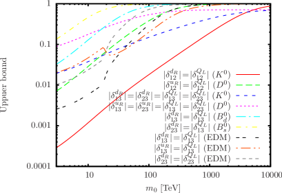
In Fig. 8, we show the constraints on some combinations of δ𝛿\delta’s. ΔΔ\Delta’s and δ𝛿\delta’s which are not displayed in the figure are set to be zero. We set the Higgsino and gauginos masses as μ=m0𝜇subscript𝑚0\mu=m_{0}, mg~=1.5subscript𝑚~𝑔1.5m_{\tilde{g}}=-1.5 TeV, mB~=+400subscript𝑚~𝐵400m_{\tilde{B}}=+400 GeV mW~=+200subscript𝑚~𝑊200m_{\tilde{W}}=+200 GeV. Here we set tanβ𝛽\tan\beta to realize the 125 GeV Higgs mass. In this estimation, we neglect the flavor violation terms and assume that all the SUSY scalar particles have a common mass m0subscript𝑚0m_{0} and that mt=173.2subscript𝑚𝑡173.2m_{t}=173.2 GeV. 666 With large flavor violating mass terms, the mass of the lightest squark can be much less than m0subscript𝑚0m_{0} and μ𝜇\mu. In this case, large finite corrections can be expected and change the prediction of the Higgs mass. In addition, if |μ|msquarkmuch-greater-than𝜇subscript𝑚squark|\mu|\gg m_{\rm squark}, the electroweak breaking vacuum may become metastable or unstable. In this paper, we neglect these effects for simplicity. In this setup, for m0<10superscriptsubscriptsubscript𝑚0similar-to10m_{0}\mathop{}_{\textstyle\sim}^{\textstyle<}10 TeV or m0>104superscriptsubscriptsubscript𝑚0similar-tosuperscript104m_{0}\mathop{}_{\textstyle\sim}^{\textstyle>}10^{4} TeV, no tanβ𝛽\tan\beta for the 125 GeV Higgs mass is found within the range of 1 to 50. In such cases, we set tanβ=50𝛽50\tan\beta=50 and 111, respectively. We also require the lightest squark is heavier than the gluino.

To get the constraints, we evaluate the one-loop box and dipole diagrams, evolve the Wilson coefficients down to relevant hadronic scales via RG equations from the QCD interaction and estimate the hadronic matrix elements. For the meson mixings, we use the results of new physics fits of Refs. [41, 42, 43] and obtain the constraints. The constraints from K0K¯0superscript𝐾0superscript¯𝐾0K^{0}-\bar{K}^{0} and D0D¯0superscript𝐷0superscript¯𝐷0D^{0}-\bar{D}^{0} mixings have large uncertainties, for lack of concrete SM predictions. In our analysis, we assume that the uncertainties of the SM predictions are same as experimental observations, e.g., δ(ΔmK)SM=(ΔmK)exp𝛿subscriptΔsubscript𝑚𝐾SMsubscriptΔsubscript𝑚𝐾exp\delta(\Delta m_{K})_{\rm SM}=(\Delta m_{K})_{\rm exp}. Although the hadronic EDMs suffer from large uncertainties, we adopt the result of Ref. [44] and compare them with the current experimental constraints [45, 46].

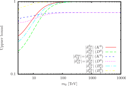
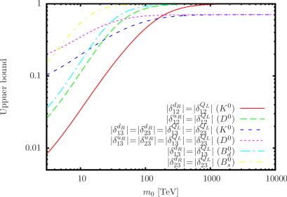
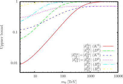
Fig. 8-(a) shows the case of flavor violation of right-handed squarks without CP-violation. Note that the constraints from K0K¯0superscript𝐾0superscript¯𝐾0K^{0}-\bar{K}^{0} and D0D¯0superscript𝐷0superscript¯𝐷0D^{0}-\bar{D}^{0} suffer from large ambiguities, depending on the treatment of the SM predictions. Fig. 8-(b) shows the case of flavor violation of both left and right-handed squarks without CP-violation. Generally, compared with the case of (a), the constraints get severer. Fig. 8-(c) shows the case of flavor violation of only right-handed squarks with CP-violation. We choose the CP-phase so that the strongest constraint can be obtained. In this case, the constraint from ϵKsubscriptitalic-ϵ𝐾\epsilon_{K} is strong and robust. Fig. 8-(d) shows the case of both left and right-handed flavor violation and CP-violation. In this case, we see that even PeV-scale SUSY suffers from strong constraints from the K0K¯0superscript𝐾0superscript¯𝐾0K^{0}-\bar{K}^{0} mixing. Here we show that the EDMs also give powerful constraints on the flavor violation. However note that these constraints strongly depend on the size of μ𝜇\mu, tanβ𝛽\tan\beta and hadronic uncertainties.

Refer to caption
(a) CP + R
Refer to caption
(b) CP + LR
Refer to caption
(c) CPV + R
Refer to caption
(d) CPV + LR
Figure 8: Upper-bound on the flavor violating mass terms δ𝛿\delta. See text for explanation.

3.2 Flavorful Gluino Decay

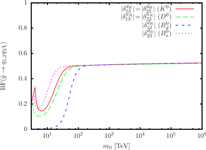
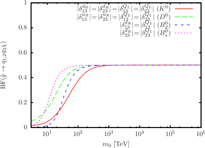
As discussed in Section 2, the flavor violating gluino decay can be expected for the squark flavor violation. As in Fig. 8, if the squark mass is larger than 𝒪(100)𝒪100{\cal O}(100) TeV, large flavor violation is allowed from the current constraints. Generally, there are gluino decays (g~q1q2χ~𝑔subscript𝑞1subscript𝑞2𝜒\tilde{g}\to q_{1}q_{2}\chi) violating both the first and second flavor violation which comes from either minimal or non-minimal flavor violation. However, instead, we focus on the gluino decays accompanied with third flavor violation (g~q1,2q3χ~𝑔subscript𝑞12subscript𝑞3𝜒\tilde{g}\to q_{1,2}q_{3}\chi), since these constraints are weak and third-family violating gluino decay may be experimentally more viable to be discovered.

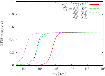
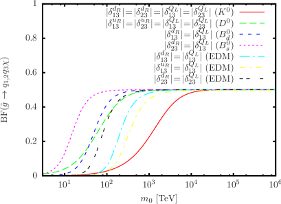
Using the same setup in Fig. 8, we show the upper-bound on the branching fraction of g~q1,2q3χ~𝑔subscript𝑞12subscript𝑞3𝜒\tilde{g}\to q_{1,2}q_{3}\chi, keeping the current experimental constraints in Fig. 9. We adopt the lightest squark mass as the boundary scale m~~𝑚\tilde{m}. As the squark mass scale m0subscript𝑚0m_{0} gets larger, the larger flavor violation δ𝛿\delta’s are allowed. In the case of the large δ𝛿\delta’s, the lightest squarks, which are mixed states of different generations, dominate the gluino decay process and the flavor violating branching fraction approximates 50 %. Except for the constraints from ϵKsubscriptitalic-ϵ𝐾\epsilon_{K}, the squark mass scale higher than 𝒪(1023)𝒪superscript1023{\cal O}(10^{2-3}) TeV can saturate the gluino flavor violating branching fraction. As m0subscript𝑚0m_{0} is larger, the RG evolution effects get more efficient and logarithmically enhance this fraction.
Refer to caption
(a) CP + R
Refer to caption
(b) CP + LR
Refer to caption
(c) CPV + R
Refer to caption
(d) CPV + LR
Figure 9: Upper-bound on the gluino branching fraction with third-family flavor violation.

4 Collider Signature

Let us briefly discuss the collider signature of the gluino decay in the high-scale SUSY models. Distinctive features of the gluino decay in the high-scale SUSY models are the longevity of the gluino lifetime and the flavor violating decay modes. The signatures of the long-lived gluinos are often discussed in the high-scale SUSY scenarios and leave unique signatures [47, 48]. Instead we focus on the signals of the flavorful gluino decay. Depending on the lifetime of the gluino, the way to identify the flavorful gluino decay differs.

Case I. cτg~𝒪(1)mmmuch-less-than𝑐subscript𝜏~𝑔𝒪1mmc\tau_{\tilde{g}}\ll{\cal O}(1)~{}{\rm mm} (m~<𝒪(103)TeV~𝑚𝒪superscript103TeV\tilde{m}<{\cal O}(10^{3})~{}{\rm TeV})


In this case, the impact parameters of the gluino decay products are less than the limitation of the LHC detector. Therefore it is difficult to directly measure the gluino lifetime. Instead, in this case, conventional collider techniques such as heavy-flavor quark and lepton tagging, jet reconstructions and so on are available. Depending on the gluino decay mode, distinctive signatures can be expected [49]. Using, for instance, the techniques developed in Ref. [32], we can estimate the gluino branching fractions.

Case I​I. 𝒪(1)mm<cτg~<𝒪(10)m𝒪1mm𝑐subscript𝜏~𝑔𝒪10m{\cal O}(1)~{}{\rm mm}<c\tau_{\tilde{g}}<{\cal O}(10)~{}{\rm m} (𝒪(103)TeV<m~<𝒪(104)TeV𝒪superscript103TeV~𝑚𝒪superscript104TeV{\cal O}(10^{3})~{}{\rm TeV}<\tilde{m}<{\cal O}(10^{4})~{}{\rm TeV})


In this case, although the gluino can decay inside the detector, some of traditional collider techniques will fail. For example, usage of the conventional b𝑏b-tagging is doubtful, since it owes to impact parameters of the b𝑏b decays. However, studies of collider signatures with displaced vertices are developing. We expect the detailed analysis of track reconstructions and energy deposit in detectors can reveal the displaced gluino decays.

Case I​I​I. cτg~𝒪(10)mmuch-greater-than𝑐subscript𝜏~𝑔𝒪10mc\tau_{\tilde{g}}\gg{\cal O}(10)~{}{\rm m} (m~𝒪(104)TeVmuch-greater-than~𝑚𝒪superscript104TeV\tilde{m}\gg{\cal O}(10^{4})~{}{\rm TeV})


In this case, the detection of in-flight decays of the gluinos is difficult. However, if a number of gluinos are produced, some of the gluinos can be trapped in the detector [50]. Information of the energy deposit in the gluino decay may be helpful, as discussed in the context of measurement of the branching fraction of the trapped staus [51]. For instance, t𝑡t quarks from the gluino decay emit leptons, which change hadronic energy deposit of the gluino decay. Therefore a detailed study of the energy deposit of the stopped gluino decay gives us a clue for the gluino decay mode.

Once the gluino decays can be fully identified, ideally, 𝒪(104)𝒪superscript104{\cal O}(10^{4}) gluino decays may result in 𝒪(1)𝒪1{\cal O}(1) % accuracy of the measurement of the gluino branching fractions. However it is unclear whether we can identify the gluino decay, eliminating the background. The detailed analysis is beyond the scope of this paper and will be done elsewhere [52].

5 Conclusion and Discussion

The framework of high-scale SUSY models is well motivated from both phenomenological and theoretical viewpoints. In particular the MSSM with the scalar scale 𝒪(10106)𝒪10superscript106{\cal O}(10-10^{6}) TeV can explain the Higgs boson with a mass of about 125 GeV. In such a framework, while the SUSY particles in the electroweak scale have a rather simple spectrum and can be accessible by experiments, the structure of the sfermion sector has strong model dependence and cannot be directly probed by the experiments. Examining the sfermion sector is essential to discriminate the underlying model. In this paper, we have discussed the gluino decay as a probe of the sfermion sector in a high-scale SUSY model. We have studied the relation between the squark sector and the gluino decay in detail.

If the gaugino mass scale is within the reach of a collider, we can observe the gluino decay which is strongly affected by the squark sector. The gluino lifetime reflects the squark scale and the decay products are sensitive to the squark flavor structure. Therefore the gluino decay will provide us clues to investigate the heavy sfermion sector. Especially, in our study, we focused on the flavor structure of the gluino decay and investigated the correlation with low-energy observations.

The large mass hierarchy between the sfermion and gaugino scale can result in large quantum corrections for the gluino decay. We have used RG methods to tame the quantum corrections. We have found that the squark mass scale is higher than 𝒪(100)𝒪100{\cal O}(100) TeV, the quantum corrections can affect the branching ratio by 𝒪(10)𝒪10{\cal O}(10) %, compared to the tree-level results. Ideally, by observing 𝒪(104)𝒪superscript104{\cal O}(10^{4}) gluino decays at a collider, we can estimate the branching fraction with 𝒪(1)𝒪1{\cal O}(1) % accuracy. Compared to this accuracy, the effects of the quantum corrections are more significant, when we try to reconstruct the squark sector via measurement of the gluino decays.

We also discussed the correlation between the gluino decay and low-energy flavor/CP observations. From the current constraints from the flavor/CP, we have found that the scalar scale 𝒪(10106)𝒪10superscript106{\cal O}(10-10^{6}) TeV allows large flavor violating gluino decay. Unlike the flavor structure of the gluino decay products, measurement of CP violation of the gluino decay seems hard. On the other hand, (future) low-energy flavor/CP experiments are sensitive to such CP violation. The combination of the gluino decay, the lifetime and decay modes, and low-energy flavor/CP observations is crucially important for the study of the underlying flavor/CP symmetry of SSMs.

In this study, we focus on the flavor structure of the quark sector. Recently, flavor violation of a leptonic sector in a high-scale SUSY model is also studied [53]. Combining these sfermion information will provide us a hint for an underlying flavor and GUT model.

Acknowledgements

SS thanks L. Hall and Y. Nomura for fruitful discussion. The work of RS and KT is supported in part by JSPS Research Fellowships for Young Scientists. This work is also supported by the World Premier International Research Center Initiative (WPI Initiative), MEXT, Japan.

Appendix A Note on Flavor Basis

In this Appendix, we summarize notations of the flavor structure which is used in this paper. We neglect A𝐴A-terms of squarks, then, the flavor dependent terms in the Lagrangian is written as,

Yukawa+softsubscriptYukawasubscriptsoft\displaystyle{\cal L}_{\rm Yukawa}+{\cal L}_{\rm soft} =(HQLYuuRc+HQLYddRc+h.c.)Q~LmQ~L2Q~Lu~Rcmu~R2u~Rcd~Rcmd~R2d~Rc,\displaystyle=(HQ_{L}Y_{u}u_{R}^{c}+H^{*}Q_{L}Y_{d}d_{R}^{c}+h.c.)-{\tilde{Q}_{L}}^{*}m^{2}_{\tilde{Q}_{L}}{\tilde{Q}_{L}}-{\tilde{u}_{R}}^{c}m^{2}_{\tilde{u}_{R}}{\tilde{u}_{R}^{c*}}-{\tilde{d}_{R}}^{c}m^{2}_{\tilde{d}_{R}}{\tilde{d}_{R}^{c*}}, (65)

A.1 Weak Basis

We can redefine quark and squark fields by using SU(2)L×U(1)Y𝑆𝑈subscript2𝐿𝑈subscript1𝑌SU(2)_{L}\times U(1)_{Y} symmetric redefinition.

QL,iQL,i=UijQQL,j,subscript𝑄𝐿𝑖subscriptsuperscript𝑄𝐿𝑖superscriptsubscript𝑈𝑖𝑗𝑄subscript𝑄𝐿𝑗\displaystyle Q_{L,i}\to Q^{\prime}_{L,i}=U_{ij}^{Q}Q_{L,j},\qquad Q~L,iQ~L,i=UijQQ~L,j,subscript~𝑄𝐿𝑖subscriptsuperscript~𝑄𝐿𝑖superscriptsubscript𝑈𝑖𝑗𝑄subscript~𝑄𝐿𝑗\displaystyle\tilde{Q}_{L,i}\to\tilde{Q}^{\prime}_{L,i}=U_{ij}^{Q}\tilde{Q}_{L,j}, (66)
uR,icuR,ic=UijuuL,jc,superscriptsubscript𝑢𝑅𝑖𝑐superscriptsuperscriptsubscript𝑢𝑅𝑖𝑐superscriptsubscript𝑈𝑖𝑗𝑢superscriptsubscript𝑢𝐿𝑗𝑐\displaystyle u_{R,i}^{c}\to{u_{R,i}^{c}}^{\prime}=U_{ij}^{u}u_{L,j}^{c},\qquad u~R,icuR,ic~=Uijuu~R,jc,superscriptsubscript~𝑢𝑅𝑖𝑐superscript~superscriptsubscript𝑢𝑅𝑖𝑐superscriptsubscript𝑈𝑖𝑗𝑢superscriptsubscript~𝑢𝑅𝑗𝑐\displaystyle\tilde{u}_{R,i}^{c}\to\tilde{u_{R,i}^{c}}^{\prime}=U_{ij}^{u}\tilde{u}_{R,j}^{c}, (67)
dR,icdR,ic=UijddL,jc,superscriptsubscript𝑑𝑅𝑖𝑐superscriptsuperscriptsubscript𝑑𝑅𝑖𝑐superscriptsubscript𝑈𝑖𝑗𝑑superscriptsubscript𝑑𝐿𝑗𝑐\displaystyle d_{R,i}^{c}\to{d_{R,i}^{c}}^{\prime}=U_{ij}^{d}d_{L,j}^{c},\qquad d~R,icdR,ic~=Uijdd~R,jc.superscriptsubscript~𝑑𝑅𝑖𝑐superscript~superscriptsubscript𝑑𝑅𝑖𝑐superscriptsubscript𝑈𝑖𝑗𝑑superscriptsubscript~𝑑𝑅𝑗𝑐\displaystyle\tilde{d}_{R,i}^{c}\to\tilde{d_{R,i}^{c}}^{\prime}=U_{ij}^{d}\tilde{d}_{R,j}^{c}. (68)

By using the above redefinition, we take a basis in which Yukawa matrices at electroweak scale is given as,

Yu=VCKMTdiag(yu,yc,yt),Yd=diag(yd,ys,yb).formulae-sequencesubscript𝑌𝑢superscriptsubscript𝑉CKM𝑇diagsubscript𝑦𝑢subscript𝑦𝑐subscript𝑦𝑡subscript𝑌𝑑diagsubscript𝑦𝑑subscript𝑦𝑠subscript𝑦𝑏\displaystyle Y_{u}=V_{\rm CKM}^{T}{\rm diag}(y_{u},y_{c},y_{t}),\qquad Y_{d}={\rm diag}(y_{d},y_{s},y_{b}). (69)

Note on that RG evolution of Yukawa matrices destroys the above form except for electroweak scale because we take scale independent U𝑈U’s. We denote this basis as “weak basis” in this paper. In this basis, we can write interaction terms as SU(2)L𝑆𝑈subscript2𝐿SU(2)_{L} symmetric forms, then, this basis is convenient to calculate the RG equations.

A.2 Super-CKM basis

In this basis, Yukawa interaction of quarks are diagonalized at electroweak scale. Quarks and squarks in this basis are related to ones in weak-basis as,

u^L=VCKMuL,u^Rc=uRc,d^L=dL,d^Rc=dRc,formulae-sequencesubscript^𝑢𝐿subscript𝑉CKMsubscript𝑢𝐿formulae-sequencesuperscriptsubscript^𝑢𝑅𝑐superscriptsubscript𝑢𝑅𝑐formulae-sequencesubscript^𝑑𝐿subscript𝑑𝐿superscriptsubscript^𝑑𝑅𝑐superscriptsubscript𝑑𝑅𝑐\displaystyle\hat{u}_{L}=V_{\rm CKM}u_{L},\qquad\hat{u}_{R}^{c}=u_{R}^{c},\qquad\hat{d}_{L}=d_{L},\qquad\hat{d}_{R}^{c}=d_{R}^{c}, (70)
u~^L=VCKMu~L,u~^Rc=u~Rc,d~^L=d~L,d~^Rc=d~Rc.formulae-sequencesubscript^~𝑢𝐿subscript𝑉CKMsubscript~𝑢𝐿formulae-sequencesuperscriptsubscript^~𝑢𝑅𝑐superscriptsubscript~𝑢𝑅𝑐formulae-sequencesubscript^~𝑑𝐿subscript~𝑑𝐿superscriptsubscript^~𝑑𝑅𝑐superscriptsubscript~𝑑𝑅𝑐\displaystyle\hat{\tilde{u}}_{L}=V_{\rm CKM}\tilde{u}_{L},\qquad\hat{\tilde{u}}_{R}^{c}=\tilde{u}_{R}^{c},\qquad\hat{\tilde{d}}_{L}=\tilde{d}_{L},\qquad\hat{\tilde{d}}_{R}^{c}=\tilde{d}_{R}^{c}. (71)

Each quark is mass eigenstate, and each squark is defined as a super-partner of each quark. In this basis, mass-squared matrices of squarks are given by,

softsubscriptsoft\displaystyle{\cal L}_{\rm soft} =u~^Lm^u~L2u~^Ld~^Lm^d~L2d~^Lu~^Rcm^u~R2u~^Rcd~^Rcm^d~R2d~^Rc,absentsuperscriptsubscript^~𝑢𝐿subscriptsuperscript^𝑚2subscript~𝑢𝐿subscript^~𝑢𝐿superscriptsubscript^~𝑑𝐿subscriptsuperscript^𝑚2subscript~𝑑𝐿subscript^~𝑑𝐿superscriptsubscript^~𝑢𝑅𝑐subscriptsuperscript^𝑚2subscript~𝑢𝑅superscriptsubscript^~𝑢𝑅𝑐superscriptsubscript^~𝑑𝑅𝑐subscriptsuperscript^𝑚2subscript~𝑑𝑅superscriptsubscript^~𝑑𝑅𝑐\displaystyle=-\hat{\tilde{u}}_{L}^{*}\hat{m}^{2}_{\tilde{u}_{L}}\hat{\tilde{u}}_{L}-\hat{\tilde{d}}_{L}^{*}\hat{m}^{2}_{\tilde{d}_{L}}\hat{\tilde{d}}_{L}-\hat{\tilde{u}}_{R}^{c}\hat{m}^{2}_{\tilde{u}_{R}}\hat{\tilde{u}}_{R}^{c*}-\hat{\tilde{d}}_{R}^{c}\hat{m}^{2}_{\tilde{d}_{R}}\hat{\tilde{d}}_{R}^{c*}, (72)

where,

m^u~L2=VCKMmQ~L2VCKM,m^d~L2=mQ~L2,m^u~R2=mu~R2,m^d~R2=md~R2.formulae-sequencesuperscriptsubscript^𝑚subscript~𝑢𝐿2subscript𝑉CKMsuperscriptsubscript𝑚subscript~𝑄𝐿2superscriptsubscript𝑉CKMformulae-sequencesuperscriptsubscript^𝑚subscript~𝑑𝐿2superscriptsubscript𝑚subscript~𝑄𝐿2formulae-sequencesuperscriptsubscript^𝑚subscript~𝑢𝑅2superscriptsubscript𝑚subscript~𝑢𝑅2superscriptsubscript^𝑚subscript~𝑑𝑅2superscriptsubscript𝑚subscript~𝑑𝑅2\displaystyle\hat{m}_{\tilde{u}_{L}}^{2}=V_{\rm CKM}m_{\tilde{Q}_{L}}^{2}V_{\rm CKM}^{\dagger},\qquad\hat{m}_{\tilde{d}_{L}}^{2}=m_{\tilde{Q}_{L}}^{2},\qquad\hat{m}_{\tilde{u}_{R}}^{2}=m_{\tilde{u}_{R}}^{2},\qquad\hat{m}_{\tilde{d}_{R}}^{2}=m_{\tilde{d}_{R}}^{2}. (73)

Appendix B RG Equations for Wilson Coefficients of Higgsinos

In some high-scale SUSY models, the Higgsino mass is also much smaller than the sfermion and heavy Higgs boson masses. If the gluino is heavier than the Higgsinos, it can decay into the Higgsino. Such decay processes are induced by the following dimension six effective interactions:

Q1u,ijH~subscriptsuperscript𝑄~𝐻1𝑢𝑖𝑗\displaystyle Q^{\tilde{H}}_{1u,ij} =\displaystyle= (H~ug~)(QL,iuR,jc),subscript~𝐻𝑢~𝑔subscript𝑄𝐿𝑖superscriptsubscript𝑢𝑅𝑗𝑐\displaystyle(\tilde{H}_{u}\tilde{g})(Q_{L,i}u_{R,j}^{c}), (74)
Q2u,ijH~subscriptsuperscript𝑄~𝐻2𝑢𝑖𝑗\displaystyle Q^{\tilde{H}}_{2u,ij} =\displaystyle= (H~uσμνg~)(QL,iσμνuR,jc),subscript~𝐻𝑢superscript𝜎𝜇𝜈~𝑔subscript𝑄𝐿𝑖subscript𝜎𝜇𝜈superscriptsubscript𝑢𝑅𝑗𝑐\displaystyle(\tilde{H}_{u}\sigma^{\mu\nu}\tilde{g})(Q_{L,i}\sigma_{\mu\nu}u_{R,j}^{c}), (75)
Q5uH~subscriptsuperscript𝑄~𝐻5𝑢\displaystyle Q^{\tilde{H}}_{5u} =\displaystyle= (H~uσμνg~)HGμν,subscript~𝐻𝑢superscript𝜎𝜇𝜈~𝑔𝐻subscript𝐺𝜇𝜈\displaystyle(\tilde{H}_{u}\sigma^{\mu\nu}\tilde{g})HG_{\mu\nu}, (76)
Q1d,ijH~subscriptsuperscript𝑄~𝐻1𝑑𝑖𝑗\displaystyle Q^{\tilde{H}}_{1d,ij} =\displaystyle= (H~dg~)(QL,idR,jc),subscript~𝐻𝑑~𝑔subscript𝑄𝐿𝑖superscriptsubscript𝑑𝑅𝑗𝑐\displaystyle(\tilde{H}_{d}\tilde{g})(Q_{L,i}d_{R,j}^{c}), (77)
Q2d,ijH~subscriptsuperscript𝑄~𝐻2𝑑𝑖𝑗\displaystyle Q^{\tilde{H}}_{2d,ij} =\displaystyle= (H~dσμνg~)(QL,iσμνdR,jc),subscript~𝐻𝑑superscript𝜎𝜇𝜈~𝑔subscript𝑄𝐿𝑖subscript𝜎𝜇𝜈superscriptsubscript𝑑𝑅𝑗𝑐\displaystyle(\tilde{H}_{d}\sigma^{\mu\nu}\tilde{g})(Q_{L,i}\sigma_{\mu\nu}d_{R,j}^{c}), (78)
Q5dH~subscriptsuperscript𝑄~𝐻5𝑑\displaystyle Q^{\tilde{H}}_{5d} =\displaystyle= (H~dσμνg~)HGμν.subscript~𝐻𝑑superscript𝜎𝜇𝜈~𝑔superscript𝐻subscript𝐺𝜇𝜈\displaystyle(\tilde{H}_{d}\sigma^{\mu\nu}\tilde{g})H^{*}G_{\mu\nu}. (79)

Dimensionless couplings in MSSM respect PQ-symmetry, then, at the leading order, we do not have to consider PQ-breaking operators, e.g., (H~dg~)(qL,iuR,jc)subscript~𝐻𝑑~𝑔superscriptsubscript𝑞𝐿𝑖superscriptsubscript𝑢𝑅𝑗𝑐(\tilde{H}_{d}\tilde{g})(q_{L,i}u_{R,j}^{c})^{\dagger}. The effective Lagrangian contains the following interaction terms:

effsubscripteff\displaystyle{\cal L}_{\rm eff} =\displaystyle= 1m~2[i,j(C1u,ijH~Q1u,ijH~+C2u,ijH~Q2u,ijH~+C1d,ijH~Q1d,ijH~+C2d,ijH~Q2d,ijH~)\displaystyle\frac{1}{\tilde{m}^{2}}\Biggl{[}\sum_{i,j}\left(C^{\tilde{H}}_{1u,ij}Q^{\tilde{H}}_{1u,ij}+C^{\tilde{H}}_{2u,ij}Q^{\tilde{H}}_{2u,ij}+C^{\tilde{H}}_{1d,ij}Q^{\tilde{H}}_{1d,ij}+C^{\tilde{H}}_{2d,ij}Q^{\tilde{H}}_{2d,ij}\right) (80)
+C5uH~Q5uH~+C5dH~Q5dH~]+h.c..\displaystyle\quad\quad\quad+C^{\tilde{H}}_{5u}Q^{\tilde{H}}_{5u}+C^{\tilde{H}}_{5d}Q^{\tilde{H}}_{5d}\Biggr{]}+h.c..

The boundary conditions at the squark mass scale m~~𝑚\tilde{m} are given by,

C1uH~(m~)subscriptsuperscript𝐶~𝐻1𝑢~𝑚\displaystyle C^{\tilde{H}}_{1u}(\tilde{m}) =\displaystyle= gs2sinβm~2[(mQ~L2)1YuYu((mu~R2)1)T],subscript𝑔𝑠2𝛽superscript~𝑚2delimited-[]superscriptsuperscriptsubscript𝑚subscript~𝑄𝐿21subscript𝑌𝑢subscript𝑌𝑢superscriptsuperscriptsuperscriptsubscript𝑚subscript~𝑢𝑅21𝑇\displaystyle\frac{g_{s}}{\sqrt{2}\sin\beta}\tilde{m}^{2}\left[(m_{\tilde{Q}_{L}}^{2})^{-1}Y_{u}-Y_{u}((m_{\tilde{u}_{R}}^{2})^{-1})^{T}\right], (81)
C2uH~(m~)subscriptsuperscript𝐶~𝐻2𝑢~𝑚\displaystyle C^{\tilde{H}}_{2u}(\tilde{m}) =\displaystyle= gs42sinβm~2[(mQ~L2)1Yu+Yu((mu~R2)1)T],subscript𝑔𝑠42𝛽superscript~𝑚2delimited-[]superscriptsuperscriptsubscript𝑚subscript~𝑄𝐿21subscript𝑌𝑢subscript𝑌𝑢superscriptsuperscriptsuperscriptsubscript𝑚subscript~𝑢𝑅21𝑇\displaystyle\frac{g_{s}}{4\sqrt{2}\sin\beta}\tilde{m}^{2}\left[(m_{\tilde{Q}_{L}}^{2})^{-1}Y_{u}+Y_{u}((m_{\tilde{u}_{R}}^{2})^{-1})^{T}\right], (82)
C5uH~(m~)subscriptsuperscript𝐶~𝐻5𝑢~𝑚\displaystyle C^{\tilde{H}}_{5u}(\tilde{m}) =\displaystyle= gs2322π2sinβm~2(tr[YuYu(mQ~L2)1]+tr[YuYuT(mu~R2)1]),superscriptsubscript𝑔𝑠2322superscript𝜋2𝛽superscript~𝑚2trdelimited-[]subscript𝑌𝑢superscriptsubscript𝑌𝑢superscriptsuperscriptsubscript𝑚subscript~𝑄𝐿21trdelimited-[]superscriptsubscript𝑌𝑢superscriptsubscript𝑌𝑢𝑇superscriptsuperscriptsubscript𝑚subscript~𝑢𝑅21\displaystyle\frac{g_{s}^{2}}{32\sqrt{2}\pi^{2}\sin\beta}\tilde{m}^{2}\left({\rm tr}[Y_{u}Y_{u}^{\dagger}(m_{\tilde{Q}_{L}}^{2})^{-1}]+{\rm tr}[Y_{u}^{*}Y_{u}^{T}(m_{\tilde{u}_{R}}^{2})^{-1}]\right), (83)
C1dH~(m~)subscriptsuperscript𝐶~𝐻1𝑑~𝑚\displaystyle C^{\tilde{H}}_{1d}(\tilde{m}) =\displaystyle= gs2cosβm~2[(mQ~L2)1YdYd((md~R2)1)T],subscript𝑔𝑠2𝛽superscript~𝑚2delimited-[]superscriptsuperscriptsubscript𝑚subscript~𝑄𝐿21subscript𝑌𝑑subscript𝑌𝑑superscriptsuperscriptsuperscriptsubscript𝑚subscript~𝑑𝑅21𝑇\displaystyle\frac{g_{s}}{\sqrt{2}\cos\beta}\tilde{m}^{2}\left[(m_{\tilde{Q}_{L}}^{2})^{-1}Y_{d}-Y_{d}((m_{\tilde{d}_{R}}^{2})^{-1})^{T}\right], (84)
C2dH~(m~)subscriptsuperscript𝐶~𝐻2𝑑~𝑚\displaystyle C^{\tilde{H}}_{2d}(\tilde{m}) =\displaystyle= gs42cosβm~2[(mQ~L2)1Yd+Yd((md~R2)1)T],subscript𝑔𝑠42𝛽superscript~𝑚2delimited-[]superscriptsuperscriptsubscript𝑚subscript~𝑄𝐿21subscript𝑌𝑑subscript𝑌𝑑superscriptsuperscriptsuperscriptsubscript𝑚subscript~𝑑𝑅21𝑇\displaystyle-\frac{g_{s}}{4\sqrt{2}\cos\beta}\tilde{m}^{2}\left[(m_{\tilde{Q}_{L}}^{2})^{-1}Y_{d}+Y_{d}((m_{\tilde{d}_{R}}^{2})^{-1})^{T}\right], (85)
C5dH~(m~)subscriptsuperscript𝐶~𝐻5𝑑~𝑚\displaystyle C^{\tilde{H}}_{5d}(\tilde{m}) =\displaystyle= gs2322π2cosβm~2(tr[YdYd(mQ~L2)1]+tr[YdYdT(md~R2)1]).superscriptsubscript𝑔𝑠2322superscript𝜋2𝛽superscript~𝑚2trdelimited-[]subscript𝑌𝑑superscriptsubscript𝑌𝑑superscriptsuperscriptsubscript𝑚subscript~𝑄𝐿21trdelimited-[]superscriptsubscript𝑌𝑑superscriptsubscript𝑌𝑑𝑇superscriptsuperscriptsubscript𝑚subscript~𝑑𝑅21\displaystyle\frac{g_{s}^{2}}{32\sqrt{2}\pi^{2}\cos\beta}\tilde{m}^{2}\left({\rm tr}[Y_{d}Y_{d}^{\dagger}(m_{\tilde{Q}_{L}}^{2})^{-1}]+{\rm tr}[Y_{d}^{*}Y_{d}^{T}(m_{\tilde{d}_{R}}^{2})^{-1}]\right). (86)

The RG equations for the Wilson coefficients CH~superscript𝐶~𝐻C^{\tilde{H}}’s are given by,

16π2dC1uH~dlogμ16superscript𝜋2𝑑subscriptsuperscript𝐶~𝐻1𝑢𝑑𝜇\displaystyle 16\pi^{2}\frac{dC^{\tilde{H}}_{1u}}{d\log\mu} =\displaystyle= 3gs2NCC1uH~+12(YuYu+YdYd)C1uH~+C1uH~YuYu,3superscriptsubscript𝑔𝑠2subscript𝑁𝐶subscriptsuperscript𝐶~𝐻1𝑢12subscript𝑌𝑢superscriptsubscript𝑌𝑢subscript𝑌𝑑superscriptsubscript𝑌𝑑subscriptsuperscript𝐶~𝐻1𝑢subscriptsuperscript𝐶~𝐻1𝑢superscriptsubscript𝑌𝑢subscript𝑌𝑢\displaystyle\frac{3g_{s}^{2}}{N_{C}}C^{\tilde{H}}_{1u}+\frac{1}{2}(Y_{u}Y_{u}^{\dagger}+Y_{d}Y_{d}^{\dagger})C^{\tilde{H}}_{1u}+C^{\tilde{H}}_{1u}Y_{u}^{\dagger}Y_{u}, (87)
16π2dC2uH~dlogμ16superscript𝜋2𝑑subscriptsuperscript𝐶~𝐻2𝑢𝑑𝜇\displaystyle 16\pi^{2}\frac{dC^{\tilde{H}}_{2u}}{d\log\mu} =\displaystyle= (4NC+1NC)gs2C2uH~+12(YuYu+YdYd)C2uH~+C2uH~YuYu+2gsYuC5uH~,4subscript𝑁𝐶1subscript𝑁𝐶superscriptsubscript𝑔𝑠2subscriptsuperscript𝐶~𝐻2𝑢12subscript𝑌𝑢superscriptsubscript𝑌𝑢subscript𝑌𝑑superscriptsubscript𝑌𝑑subscriptsuperscript𝐶~𝐻2𝑢subscriptsuperscript𝐶~𝐻2𝑢superscriptsubscript𝑌𝑢subscript𝑌𝑢2subscript𝑔𝑠subscript𝑌𝑢subscriptsuperscript𝐶~𝐻5𝑢\displaystyle-\left(4N_{C}+\frac{1}{N_{C}}\right)g_{s}^{2}C^{\tilde{H}}_{2u}+\frac{1}{2}(Y_{u}Y_{u}^{\dagger}+Y_{d}Y_{d}^{\dagger})C^{\tilde{H}}_{2u}+C^{\tilde{H}}_{2u}Y_{u}^{\dagger}Y_{u}+2g_{s}Y_{u}C^{\tilde{H}}_{5u}, (88)
16π2dC5uH~dlogμ16superscript𝜋2𝑑subscriptsuperscript𝐶~𝐻5𝑢𝑑𝜇\displaystyle 16\pi^{2}\frac{dC^{\tilde{H}}_{5u}}{d\log\mu} =\displaystyle= (23NF6NC)gs2C5uH~+NCtr[YuYu+YdYd]C5uH~+4gstr[C2uYu],23subscript𝑁𝐹6subscript𝑁𝐶superscriptsubscript𝑔𝑠2subscriptsuperscript𝐶~𝐻5𝑢subscript𝑁𝐶trdelimited-[]subscript𝑌𝑢superscriptsubscript𝑌𝑢subscript𝑌𝑑superscriptsubscript𝑌𝑑subscriptsuperscript𝐶~𝐻5𝑢4subscript𝑔𝑠trdelimited-[]subscript𝐶2𝑢superscriptsubscript𝑌𝑢\displaystyle\left(\frac{2}{3}N_{F}-6N_{C}\right)g_{s}^{2}C^{\tilde{H}}_{5u}+N_{C}{\rm tr}\left[Y_{u}Y_{u}^{\dagger}+Y_{d}Y_{d}^{\dagger}\right]C^{\tilde{H}}_{5u}+4g_{s}{\rm tr}\left[C_{2u}Y_{u}^{\dagger}\right], (89)
16π2dC1dH~dlogμ16superscript𝜋2𝑑subscriptsuperscript𝐶~𝐻1𝑑𝑑𝜇\displaystyle 16\pi^{2}\frac{dC^{\tilde{H}}_{1d}}{d\log\mu} =\displaystyle= 3gs2NCC1dH~+12(YuYu+YdYd)C1dH~+C1dH~YdYd,3superscriptsubscript𝑔𝑠2subscript𝑁𝐶subscriptsuperscript𝐶~𝐻1𝑑12subscript𝑌𝑢superscriptsubscript𝑌𝑢subscript𝑌𝑑superscriptsubscript𝑌𝑑subscriptsuperscript𝐶~𝐻1𝑑subscriptsuperscript𝐶~𝐻1𝑑superscriptsubscript𝑌𝑑subscript𝑌𝑑\displaystyle\frac{3g_{s}^{2}}{N_{C}}C^{\tilde{H}}_{1d}+\frac{1}{2}(Y_{u}Y_{u}^{\dagger}+Y_{d}Y_{d}^{\dagger})C^{\tilde{H}}_{1d}+C^{\tilde{H}}_{1d}Y_{d}^{\dagger}Y_{d}, (90)
16π2dC2dH~dlogμ16superscript𝜋2𝑑subscriptsuperscript𝐶~𝐻2𝑑𝑑𝜇\displaystyle 16\pi^{2}\frac{dC^{\tilde{H}}_{2d}}{d\log\mu} =\displaystyle= (4NC+1NC)gs2C2dH~+12(YuYu+YdYd)C2dH~+C2dH~YdYd+2gsYdC5dH~,4subscript𝑁𝐶1subscript𝑁𝐶superscriptsubscript𝑔𝑠2subscriptsuperscript𝐶~𝐻2𝑑12subscript𝑌𝑢superscriptsubscript𝑌𝑢subscript𝑌𝑑superscriptsubscript𝑌𝑑subscriptsuperscript𝐶~𝐻2𝑑subscriptsuperscript𝐶~𝐻2𝑑superscriptsubscript𝑌𝑑subscript𝑌𝑑2subscript𝑔𝑠subscript𝑌𝑑subscriptsuperscript𝐶~𝐻5𝑑\displaystyle-\left(4N_{C}+\frac{1}{N_{C}}\right)g_{s}^{2}C^{\tilde{H}}_{2d}+\frac{1}{2}(Y_{u}Y_{u}^{\dagger}+Y_{d}Y_{d}^{\dagger})C^{\tilde{H}}_{2d}+C^{\tilde{H}}_{2d}Y_{d}^{\dagger}Y_{d}+2g_{s}Y_{d}C^{\tilde{H}}_{5d}, (91)
16π2dC5dH~dlogμ16superscript𝜋2𝑑subscriptsuperscript𝐶~𝐻5𝑑𝑑𝜇\displaystyle 16\pi^{2}\frac{dC^{\tilde{H}}_{5d}}{d\log\mu} =\displaystyle= (23NF6NC)gs2C5dH~+NCtr[YuYu+YdYd]C5dH~+4gstr[C2dYd].23subscript𝑁𝐹6subscript𝑁𝐶superscriptsubscript𝑔𝑠2subscriptsuperscript𝐶~𝐻5𝑑subscript𝑁𝐶trdelimited-[]subscript𝑌𝑢superscriptsubscript𝑌𝑢subscript𝑌𝑑superscriptsubscript𝑌𝑑subscriptsuperscript𝐶~𝐻5𝑑4subscript𝑔𝑠trdelimited-[]subscript𝐶2𝑑superscriptsubscript𝑌𝑑\displaystyle\left(\frac{2}{3}N_{F}-6N_{C}\right)g_{s}^{2}C^{\tilde{H}}_{5d}+N_{C}{\rm tr}\left[Y_{u}Y_{u}^{\dagger}+Y_{d}Y_{d}^{\dagger}\right]C^{\tilde{H}}_{5d}+4g_{s}{\rm tr}\left[C_{2d}Y_{d}^{\dagger}\right]. (92)

Here, we take into account only quark Yukawa and QCD interactions. We have checked Eqs. (8792) are consistent with Ref. [31] in the flavor-symmetric case. For the RG equations of dimensionless coupling constants, see the Appendix of Ref. [9].

Appendix C RG Equations of Soft Mass with Flavor Violation

In this appendix, we show the RG equations for sfermion soft masses. Here, we neglect trilinear-coupling, gaugino masses. We assume relatively small tanβ𝛽\tan\beta, then neglect down-type quark and lepton Yukawa couplings.

16π2dmQ~L2dlogμ16superscript𝜋2𝑑superscriptsubscript𝑚subscript~𝑄𝐿2𝑑𝜇\displaystyle 16\pi^{2}\frac{dm_{\tilde{Q}_{L}}^{2}}{d\log\mu} =\displaystyle= 2{YuYuT,mQ~L2}+2Yu(mu~R2T+mHu2𝟏)YuT+g12S5𝟏,2superscriptsubscript𝑌𝑢superscriptsubscript𝑌𝑢𝑇superscriptsubscript𝑚subscript~𝑄𝐿22superscriptsubscript𝑌𝑢superscriptsubscript𝑚subscript~𝑢𝑅2𝑇superscriptsubscript𝑚subscript𝐻𝑢21superscriptsubscript𝑌𝑢𝑇superscriptsubscript𝑔12𝑆51\displaystyle 2\left\{Y_{u}^{*}Y_{u}^{T},m_{\tilde{Q}_{L}}^{2}\right\}+2Y_{u}^{*}(m_{\tilde{u}_{R}}^{2T}+m_{H_{u}}^{2}{\bf 1})Y_{u}^{T}+\frac{g_{1}^{2}S}{5}{\bf 1}, (93)
16π2dmu~R2dlogμ16superscript𝜋2𝑑superscriptsubscript𝑚subscript~𝑢𝑅2𝑑𝜇\displaystyle 16\pi^{2}\frac{dm_{\tilde{u}_{R}}^{2}}{d\log\mu} =\displaystyle= 4{YuYu,mu~R2}+4Yu(mQ~L2T+mHu2𝟏)Yu4g12S5𝟏,4superscriptsubscript𝑌𝑢subscript𝑌𝑢superscriptsubscript𝑚subscript~𝑢𝑅24superscriptsubscript𝑌𝑢superscriptsubscript𝑚subscript~𝑄𝐿2𝑇superscriptsubscript𝑚subscript𝐻𝑢21subscript𝑌𝑢4superscriptsubscript𝑔12𝑆51\displaystyle 4\left\{Y_{u}^{\dagger}Y_{u},m_{\tilde{u}_{R}}^{2}\right\}+4Y_{u}^{\dagger}(m_{\tilde{Q}_{L}}^{2T}+m_{H_{u}}^{2}{\bf 1})Y_{u}-\frac{4g_{1}^{2}S}{5}{\bf 1}, (94)
16π2dmd~R2dlogμ16superscript𝜋2𝑑superscriptsubscript𝑚subscript~𝑑𝑅2𝑑𝜇\displaystyle 16\pi^{2}\frac{dm_{\tilde{d}_{R}}^{2}}{d\log\mu} =\displaystyle= 2g12S5𝟏,2superscriptsubscript𝑔12𝑆51\displaystyle\frac{2g_{1}^{2}S}{5}{\bf 1}, (95)
16π2dmL~L2dlogμ16superscript𝜋2𝑑superscriptsubscript𝑚subscript~𝐿𝐿2𝑑𝜇\displaystyle 16\pi^{2}\frac{dm_{\tilde{L}_{L}}^{2}}{d\log\mu} =\displaystyle= 3g12S5𝟏,3superscriptsubscript𝑔12𝑆51\displaystyle-\frac{3g_{1}^{2}S}{5}{\bf 1}, (96)
16π2dme~R2dlogμ16superscript𝜋2𝑑superscriptsubscript𝑚subscript~𝑒𝑅2𝑑𝜇\displaystyle 16\pi^{2}\frac{dm_{\tilde{e}_{R}}^{2}}{d\log\mu} =\displaystyle= 6g12S5𝟏,6superscriptsubscript𝑔12𝑆51\displaystyle\frac{6g_{1}^{2}S}{5}{\bf 1}, (97)
16π2dmHu2dlogμ16superscript𝜋2𝑑superscriptsubscript𝑚subscript𝐻𝑢2𝑑𝜇\displaystyle 16\pi^{2}\frac{dm_{H_{u}}^{2}}{d\log\mu} =\displaystyle= 6tr[YuYuTmQ~L2]+6tr[YuYumu~R2]+6tr[YuYu]mHu2+3g12S5,6trdelimited-[]superscriptsubscript𝑌𝑢superscriptsubscript𝑌𝑢𝑇superscriptsubscript𝑚subscript~𝑄𝐿26trdelimited-[]superscriptsubscript𝑌𝑢subscript𝑌𝑢superscriptsubscript𝑚subscript~𝑢𝑅26trdelimited-[]subscript𝑌𝑢superscriptsubscript𝑌𝑢superscriptsubscript𝑚subscript𝐻𝑢23superscriptsubscript𝑔12𝑆5\displaystyle 6{\rm tr}[Y_{u}^{*}Y_{u}^{T}m_{\tilde{Q}_{L}}^{2}]+6{\rm tr}[Y_{u}^{\dagger}Y_{u}m_{\tilde{u}_{R}}^{2}]+6{\rm tr}[Y_{u}Y_{u}^{\dagger}]m_{H_{u}}^{2}+\frac{3g_{1}^{2}S}{5}, (98)
16π2dmHd2dlogμ16superscript𝜋2𝑑superscriptsubscript𝑚subscript𝐻𝑑2𝑑𝜇\displaystyle 16\pi^{2}\frac{dm_{H_{d}}^{2}}{d\log\mu} =\displaystyle= 3g12S5.3superscriptsubscript𝑔12𝑆5\displaystyle-\frac{3g_{1}^{2}S}{5}. (99)

Here, sfermion mass-squared matrices mQ~L2superscriptsubscript𝑚subscript~𝑄𝐿2m_{\tilde{Q}_{L}}^{2}, mu~R2superscriptsubscript𝑚subscript~𝑢𝑅2m_{\tilde{u}_{R}}^{2}, md~R2superscriptsubscript𝑚subscript~𝑑𝑅2m_{\tilde{d}_{R}}^{2}, mL~L2superscriptsubscript𝑚subscript~𝐿𝐿2m_{\tilde{L}_{L}}^{2} and me~R2superscriptsubscript𝑚subscript~𝑒𝑅2m_{\tilde{e}_{R}}^{2} and Yukawa matrix Yusubscript𝑌𝑢Y_{u} are 3×3333\times 3 matrices in flavor space. S=mHu2mHd2+tr[mQ22mu2+md2mL2+me2]𝑆superscriptsubscript𝑚subscript𝐻𝑢2superscriptsubscript𝑚subscript𝐻𝑑2trdelimited-[]superscriptsubscript𝑚𝑄22superscriptsubscript𝑚𝑢2superscriptsubscript𝑚𝑑2superscriptsubscript𝑚𝐿2superscriptsubscript𝑚𝑒2S=m_{H_{u}}^{2}-m_{H_{d}}^{2}+{\rm tr}\left[m_{Q}^{2}-2m_{u}^{2}+m_{d}^{2}-m_{L}^{2}+m_{e}^{2}\right]. {A,B}=AB+BA𝐴𝐵𝐴𝐵𝐵𝐴\{A,B\}=AB+BA, 𝟏=diag(1,1,1)1diag111{\bf 1}={\rm diag}(1,1,1).

References

  • [1] G. Aad et al. [ATLAS Collaboration], Phys. Lett. B 716, 1 (2012) [arXiv:1207.7214 [hep-ex]].
  • [2] S. Chatrchyan et al. [CMS Collaboration], Phys. Lett. B 716, 30 (2012) [arXiv:1207.7235 [hep-ex]].
  • [3] J. D. Wells, hep-ph/0306127.
  • [4] N. Arkani-Hamed and S. Dimopoulos, JHEP 0506, 073 (2005) [hep-th/0405159].
  • [5] G. F. Giudice and A. Romanino, Nucl. Phys. B 699, 65 (2004) [Erratum-ibid. B 706, 65 (2005)] [hep-ph/0406088].
  • [6] N. Arkani-Hamed, S. Dimopoulos, G. F. Giudice and A. Romanino, Nucl. Phys. B 709, 3 (2005) [hep-ph/0409232].
  • [7] J. D. Wells, Phys. Rev. D 71, 015013 (2005) [hep-ph/0411041].
  • [8] Y. Okada, M. Yamaguchi and T. Yanagida, Prog. Theor. Phys.  85, 1 (1991); Y. Okada, M. Yamaguchi and T. Yanagida, Phys. Lett. B 262, 54 (1991); J. R. Ellis, G. Ridolfi and F. Zwirner, Phys. Lett. B 257, 83 (1991); H. E. Haber and R. Hempfling, Phys. Rev. Lett.  66, 1815 (1991); H. E. Haber and R. Hempfling, Phys. Rev. Lett.  66, 1815 (1991); J. R. Ellis, G. Ridolfi and F. Zwirner, Phys. Lett. B 262, 477 (1991).
  • [9] G. F. Giudice and A. Strumia, Nucl. Phys. B 858, 63 (2012) [arXiv:1108.6077 [hep-ph]].
  • [10] G. F. Giudice, M. A. Luty, H. Murayama and R. Rattazzi, JHEP 9812, 027 (1998) [hep-ph/9810442]; L. Randall and R. Sundrum, Nucl. Phys. B 557, 79 (1999) [hep-th/9810155]; M. Dine and D. MacIntire, Phys. Rev. D 46, 2594 (1992) [hep-ph/9205227]; J. A. Bagger, T. Moroi and E. Poppitz, JHEP 0004, 009 (2000) [hep-th/9911029]; P. Binetruy, M. K. Gaillard and B. D. Nelson, Nucl. Phys. B 604, 32 (2001) [hep-ph/0011081].
  • [11] L. J. Hall and Y. Nomura, JHEP 1201, 082 (2012) [arXiv:1111.4519 [hep-ph]]; L. J. Hall, Y. Nomura and S. Shirai, JHEP 1301, 036 (2013) [arXiv:1210.2395 [hep-ph]].
  • [12] M. Ibe and T. T. Yanagida, Phys. Lett. B 709, 374 (2012) [arXiv:1112.2462 [hep-ph]]; M. Ibe, S. Matsumoto and T. T. Yanagida, Phys. Rev. D 85, 095011 (2012) [arXiv:1202.2253 [hep-ph]].
  • [13] A. Arvanitaki, N. Craig, S. Dimopoulos and G. Villadoro, JHEP 1302, 126 (2013) [arXiv:1210.0555 [hep-ph]].
  • [14] N. Arkani-Hamed, A. Gupta, D. E. Kaplan, N. Weiner and T. Zorawski, arXiv:1212.6971 [hep-ph].
  • [15] M. Ibe, T. Moroi and T. T. Yanagida, Phys. Lett. B 644, 355 (2007) [hep-ph/0610277]; M. R. Buckley, L. Randall and B. Shuve, JHEP 05, 097 (2011) [arXiv:0909.4549 [hep-ph]].
  • [16] S. Asai, T. Moroi, K. Nishihara and T. T. Yanagida, Phys. Lett. B 653, 81 (2007) [arXiv:0705.3086 [hep-ph]]; S. Asai, T. Moroi and T. T. Yanagida, Phys. Lett. B 664, 185 (2008) [arXiv:0802.3725 [hep-ph]]; S. Asai, Y. Azuma, O. Jinnouchi, T. Moroi, S. Shirai and T. T. Yanagida, Phys. Lett.  B 672, 339 (2009) [arXiv:0807.4987 [hep-ph]].
  • [17] T. Gherghetta, G. F. Giudice and J. D. Wells, Nucl. Phys. B 559, 27 (1999) [hep-ph/9904378]; T. Moroi and L. Randall, Nucl. Phys. B 570, 455 (2000) [hep-ph/9906527].
  • [18] J. Hisano, S. Matsumoto, O. Saito and M. Senami, Phys. Rev. D 73, 055004 (2006) [hep-ph/0511118]; J. Hisano, S. Matsumoto, M. Nagai, O. Saito and M. Senami, Phys. Lett. B 646, 34 (2007) [hep-ph/0610249].
  • [19] J. Hisano, K. Ishiwata and N. Nagata, Phys. Rev. D 82, 115007 (2010) [arXiv:1007.2601 [hep-ph]]; J. Hisano, K. Ishiwata, N. Nagata and T. Takesako, JHEP 07, 005 (2011) [arXiv:1104.0228 [hep-ph]]; R. J. Hill and M. P. Solon, Phys. Lett. B 707, 539 (2012) [arXiv:1111.0016 [hep-ph]]; J. Hisano, K. Ishiwata and N. Nagata, Phys. Rev. D 87, 035020 (2013) [arXiv:1210.5985 [hep-ph]].
  • [20] J. Hisano, S. .Matsumoto, M. M. Nojiri and O. Saito, Phys. Rev. D 71, 063528 (2005) [hep-ph/0412403].
  • [21] T. Moroi and K. Nakayama, Phys. Lett. B 710, 159 (2012) [arXiv:1112.3123 [hep-ph]].
  • [22] T. Cohen, M. Lisanti, A. Pierce and T. R. Slatyer, arXiv:1307.4082 [hep-ph].
  • [23] J. Fan and M. Reece, arXiv:1307.4400 [hep-ph].
  • [24] K. I. Izawa, Y. Nomura, K. Tobe and T. Yanagida, Phys. Rev. D 56, 2886 (1997) [hep-ph/9705228];
  • [25] Y. Nomura and K. Tobe, Phys. Rev. D 58, 055002 (1998) [hep-ph/9708377].
  • [26] Z. Komargodski and D. Shih, JHEP 0904, 093 (2009) [arXiv:0902.0030 [hep-th]].
  • [27] S. Shirai, M. Yamazaki and K. Yonekura, JHEP 1006, 056 (2010) [arXiv:1003.3155 [hep-ph]].
  • [28] M. Ibe and R. Sato, Phys. Lett. B 717, 197 (2012) [arXiv:1204.3499 [hep-ph]].
  • [29] R. Saito and S. Shirai, Phys. Lett. B 713, 237 (2012) [arXiv:1201.6589 [hep-ph]].
  • [30] M. Toharia and J. D. Wells, JHEP 0602, 015 (2006) [hep-ph/0503175].
  • [31] P. Gambino, G. F. Giudice and P. Slavich, Nucl. Phys. B 726, 35 (2005) [hep-ph/0506214].
  • [32] R. Sato, S. Shirai and K. Tobioka, JHEP 1211, 041 (2012) [arXiv:1207.3608 [hep-ph]].
  • [33] A. Arvanitaki, C. Davis, P. W. Graham, A. Pierce and J. G. Wacker, Phys. Rev. D 72, 075011 (2005) [hep-ph/0504210].
  • [34] M. E. Machacek and M. T. Vaughn, Phys. Lett. B 103, 427 (1981).
  • [35] M. Ibe, S. Matsumoto and R. Sato, Phys. Lett. B 721, 252 (2013) [arXiv:1212.5989 [hep-ph]].
  • [36] ATLAS collaboration, ATLAS-CONF-2013-069
  • [37] R. Barbieri, G. Gamberini, G. F. Giudice and G. Ridolfi, Nucl. Phys. B 301, 15 (1988);
  • [38] F. Gabbiani, E. Gabrielli, A. Masiero and L. Silvestrini, Nucl. Phys. B 477, 321 (1996) [hep-ph/9604387].
  • [39] W. Altmannshofer, A. J. Buras, S. Gori, P. Paradisi and D. M. Straub, Nucl. Phys. B 830, 17 (2010) [arXiv:0909.1333 [hep-ph]].
  • [40] D. McKeen, M. Pospelov and A. Ritz, arXiv:1303.1172 [hep-ph].
  • [41] M. Bona et al. [UTfit Collaboration], JHEP 0803, 049 (2008) [arXiv:0707.0636 [hep-ph]].
  • [42] A. J. Bevan et al. [UTfit Collaboration], JHEP 1210, 068 (2012) [arXiv:1206.6245 [hep-ph]].
  • [43] http://www.utfit.org/UTfit/ResultsWinter2013PreMoriond
  • [44] J. Hisano and Y. Shimizu, Phys. Rev. D 70, 093001 (2004) [hep-ph/0406091].
  • [45] C. A. Baker, D. D. Doyle, P. Geltenbort, K. Green, M. G. D. van der Grinten, P. G. Harris, P. Iaydjiev and S. N. Ivanov et al., Phys. Rev. Lett.  97, 131801 (2006) [hep-ex/0602020].
  • [46] W. C. Griffith, M. D. Swallows, T. H. Loftus, M. V. Romalis, B. R. Heckel and E. N. Fortson, Phys. Rev. Lett.  102, 101601 (2009).
  • [47] J. L. Hewett, B. Lillie, M. Masip and T. G. Rizzo, JHEP 0409, 070 (2004) [hep-ph/0408248].
  • [48] K. Cheung and W. -Y. Keung, Phys. Rev. D 71, 015015 (2005) [hep-ph/0408335].
  • [49] A. Bartl, H. Eberl, E. Ginina, B. Herrmann, K. Hidaka, W. Majerotto and W. Porod, Phys. Rev. D 84, 115026 (2011) [arXiv:1107.2775 [hep-ph]].
  • [50] A. Arvanitaki, S. Dimopoulos, A. Pierce, S. Rajendran and J. G. Wacker, Phys. Rev. D 76, 055007 (2007) [hep-ph/0506242].
  • [51] T. Ito, K. Nakaji and S. Shirai, Phys. Lett. B 706, 314 (2012) [arXiv:1104.2101 [hep-ph]].
  • [52] R. Sato, S. Shirai and K. Tobioka, in preparation.
  • [53] T. Moroi and M. Nagai, Phys. Lett. B 723, 107 (2013) [arXiv:1303.0668 [hep-ph]], T. Moroi, M. Nagai and T. T. Yanagida, arXiv:1305.7357 [hep-ph].