Transient ageing in fractional Brownian and Langevin equation motion

Abstract

Stochastic processes driven by stationary fractional Gaussian noise, that is, fractional Brownian motion and fractional Langevin equation motion, are usually considered to be ergodic in the sense that, after an algebraic relaxation, time and ensemble averages of physical observables coincide. Recently it was demonstrated that fractional Brownian motion and fractional Langevin equation motion under external confinement are transiently non-ergodic—time and ensemble averages behave differently—from the moment when the particle starts to sense the confinement. Here we show that these processes also exhibit transient ageing, that is, physical observables such as the time averaged mean squared displacement depend on the time lag between the initiation of the system at time $t=0$ and the start of the measurement at the ageing time $t_{a}$. In particular, it turns out that for fractional Langevin equation motion the ageing dependence on $t_{a}$ is different between the cases of free and confined motion. We obtain explicit analytical expressions for the aged moments of the particle position as well as the time averaged mean squared displacement and present a numerical analysis of this transient ageing phenomenon.

I Introduction

Normal Brownian diffusion processes are stationary in the sense that physical quantities such as two point correlation functions $C(t_{1},t_{2})$ only depend on the difference of the two times $t_{1}$ and $t_{2}$, $C(t_{1},t_{2})=C(|t_{1}-t_{2}|)$. Moreover, they are independent of the time difference $t_{a}$ between initiation of the process at $t=0$ and start of the measurement at the ageing time $t_{a}$. For anomalous diffusion processes, characterized by a mean squared displacement (MSD) of the form $\langle x^{2}(t)\rangle\simeq K_{\alpha}t^{\alpha}$ with the generalized diffusion coefficient $K_{\alpha}$ of physical dimension $\mathrm{cm}^{2}/\mathrm{sec}^{\alpha}$, stationarity is not necessarily fulfilled. In both the subdiffusive ($0<\alpha<1$) and superdiffusive ($\alpha>1$) regimes, physical observables may be non-ergodic and exhibit an explicit dependence on the ageing time $t_{a}$.

Such consequences of non-stationary behavior may be illustrated by means of the time averaged MSD

$$\overline{\delta^{2}(\Delta)}=\frac{1}{T-\Delta}\int\limits_{t_{a}}^{t_{a}+T-\Delta}\Big{[}x(t+\Delta)-x(t)\Big{]}^{2}dt.$$ (1)

It evaluates a measured single particle trajectory in terms of the sliding average along the time series $x(t)$ of length $T$ over the squared position differences as separated by the lag time $\Delta$. This definition of the time averaged MSD is typically used to analyze trajectories recorded in experiments or simulations pt ; igor . Here we denote time averages by an overline, $\overline{\,\,\,\cdot\,\,\,}$. For trajectories of finite length, the additional average over sufficiently many trajectories with label $i$, $\langle\overline{\delta^{2}(\Delta)}\rangle=(1/N)\sum_{i=1}^{N}\overline{\delta^{2}(\Delta)}_{i}$, provides a smooth functional behavior. The quantity $\overline{\delta^{2}(\Delta)}$ contrasts the more standard ensemble MSD $\langle x^{2}(t)\rangle=\int x^{2}P(x,t)dx$, defined as the spatial average of $x^{2}$ over the probability density function $P(x,t)$.

The integrand in expression (1) for the time averaged MSD $\langle\overline{\delta^{2}(\Delta)}\rangle$ of a random walk process may be expressed as the product of the typical squared length per jump, $\langle\delta x^{2}\rangle$, and the average number of jumps $\langle n(t+\Delta,t)\rangle$ performed in the time interval between $t$ and $t+\Delta$ he ; johannes . For Brownian motion, the number of jumps is given by the length of the interval, $\Delta$, divided by the typical time $\tau$ per jump, that is, $\langle n(t+\Delta,t)\rangle=\Delta/\tau$. Defining the diffusion constant as $K_{1}=\langle\delta x^{2}\rangle/[2\tau]$, after integration over $t$ we find that $\langle\overline{\delta x^{2}(\Delta)}\rangle=2K_{1}\Delta$ for any finite $T$ pccp . This result is independent of the ageing time $t_{a}$ and the length $T$ of the time series: we say that the process does not age. Moreover, it is ergodic in the sense that $\langle\delta^{2}(\Delta)\rangle=\langle x^{2}(\Delta)\rangle$. For sufficiently large $T$ the process is self-averaging in the sense that on average each jump occurs after the time increment $\tau$, and thus a single trajectory $x(t)$ produces the result $\overline{\delta x^{2}(\Delta)}=2K_{1}\Delta$ such that the time averaged MSD of different trajectories is fully reproducible he ; pccp .

In contrast, processes described by the Scher-Montroll continuous time random walk (CTRW) model with a power-law distribution $\psi(\tau)\simeq\tau^{-1-\alpha}$ ($0<\alpha<1$) of waiting times $\tau$ between successive jumps scher exhibit a so-called weak ergodicity breaking web , $\langle\delta^{2}(\Delta)\rangle\neq\langle x^{2}(\Delta)\rangle$: while the ensemble averaged MSD scales sub-linearly with time, $\langle x^{2}(t)\rangle\simeq K_{\alpha}t^{\alpha}$, the time averaged MSD is linear in the lag time, $\langle\overline{\delta^{2}(\Delta)}\rangle\simeq K_{\alpha}\Delta/T^{1-\alpha}$ but depends on the measurement time $T$ he ; ariel . Under confinement, $\langle x^{2}(t)\rangle$ reaches the thermal plateau value $\langle x^{2}\rangle_{\mathrm{th}}$ thermal , while $\overline{\delta^{2}(\Delta)}\simeq(\Delta/T)^{1-\alpha}$ continues to grow in power-law fashion pnas ; neusius . Such weakly non-ergodic dynamics in absence and presence of confinement was indeed observed experimentally in both the walls and the bulk volume of living biological cells weigel ; lene ; stas . Interestingly, a similar weak ergodicity breaking is obtained for time- and space-correlated CTRWs corr and ‘superageing’ systems michael_bus as well as for Markovian diffusion with scaling forms of the position dependence of the diffusion coefficient andrey . In superdiffusive systems the ergodic violation becomes ‘ultraweak’ in the sense that $\langle x^{2}(\Delta)\rangle$ and $\langle\overline{\delta^{2}(\Delta)}\rangle$ differ only by a constant factor zukla . Moreover, the ageing dependence on $t_{a}$ was derived for subdiffusive CTRW, in which the ageing time $t_{a}$ explicitly enters the expressions for both $\langle x^{2}(t)\rangle$ and $\overline{\delta^{2}(\Delta)}$ eli_age ; johannes . For the time averaged MSD the ageing time $t_{a}$ enters solely through a multiplicative factor, independent of the process details johannes .

Here we are interested in the ageing properties of another popular class of anomalous diffusion models: fractional Brownian motion (FBM) and fractional Langevin equation (FLE) motion are driven by stationary Gaussian but power-law correlated non-white noise and algebraically reach ergodic behavior, $\overline{\delta^{2}(\Delta)}\sim\langle x^{2}(\Delta)\rangle$ in the case of free, unconfined motion deng and $\overline{\delta^{2}(\Delta)}\sim 2\langle x^{2}\rangle_{\mathrm{th}}$ for confined motion jae ; jeon1 ; REM . FBM and FLE motion in the overdamped regime behave similarly, and both emanate as effective one-particle description in many-particle systems such as viscoelastic environments, single file diffusion, or the motion of a monomer in a long polymer chain hoefling ; goychuk ; szym ; tobias . The ergodic nature of FBM/FLE anomalous diffusion was observed for the motion of telomeres in cell nuclei bronstein , the diffusion of tracers in the cytoplasm of biological cells at sufficiently long times weber ; szym ; lene , or for the motion of simulated lipid molecules in bilayers in different physical phases jae_lipid . However, in contrast to the exponential relaxation $\langle x^{2}(t)\rangle\sim\langle x^{2}\rangle_{\mathrm{th}}(1-\mathrm{const.}t^{\alpha-2}\exp\{-\mathrm{const.^{\prime}}t\})$ of the ensemble averaged MSD under confinement, the time averaged MSD of FBM exhibit the power-law approach $\overline{\delta^{2}(\Delta)}\sim 2\langle x^{2}\rangle_{\mathrm{th}}(1-\mathrm{const.}\Delta^{\alpha-2})$ jeon1 . We call this a transiently non-ergodic behavior. Such a power-law relaxation of the time averaged MSD was recently observed experimentally for microbeads tracked by optical tweezers in a wormlike micellar solution lene1 .

Similar to the observation of weakly non-ergodic behavior in FBM or FLE motion also the transient ageing behavior of these processes may become relevant under certain experimental conditions, such that the influence of the ageing time $t_{a}$ remains detectable during the measurement. Given the temporal resolution of modern spectroscopic or single particle tracking methods, this may be possible. Even more so, this question may become relevant in simulations studies in which extremely high time resolution is possible. Here we derive the different patterns of transient ageing in the FBM/FLE family of processes fueled by power-law correlated Gaussian noise. Thus we find that the time averaged MSD splits into two additive terms: a stationary term depending solely on the lag time $\Delta$, and an ageing term that decays with both ageing time $t_{a}$ and process time $T$. For both FBM and FLE motion the dependence on the process time $T$ is inversely proportional. For confined FBM we obtain an exponentially fast decay in $t_{a}$, while for FLE motion we find an algebraic decay in the ageing time. Interestingly, the scaling exponent is different between free and confined FLE motion.

The paper is structured as follows. After a definition of fractional Gaussian noise and an introduction to the FLE and FBM in terms of their dynamic equations in Sec. II, in Secs. III to V we discuss the ensemble and time averaged moments as well as the ergodic and ageing behavior of free and confined FLE motion and confined FBM. In Sec. VI we draw our conclusions. In the Appendices we describe the simulations procedure to create stochastic trajectories $x(t)$ and collect results for the autocorrelation functions.

II Anomalous diffusion models with power-law correlated, Gaussian noise

We investigate two variants of stochastic differential equations, both driven by so-called fractional Gaussian noise. These comprise the FLE, in which the fluctuation-dissipation relation kubo is satisfied, and FBM, in which the noise is external and the motion therefore is not thermalized. The associated simulations schemes are compiled in Appendix A.

Fractional Gaussian noise, the derivative process of FBM mandelbrot ; gripenberg , has zero mean $\langle\xi_{H}(t)\rangle=0$, and the variance ($0<H<1$)

$$\langle\xi_{H}(t_{1})\xi_{H}(t_{2})\rangle = 2D_{H}H(2H-1)|t_{1}-t_{2}|^{2H-2}$$ (2)

$$+ 4D_{H}H|t_{2}-t_{1}|^{2H-1}\delta(t_{2}-t_{1}),$$

exhibiting a power-law decay with scaling exponent $2H-2$ of the difference between the two times $t_{1}$ and $t_{2}$. Here, $H$ denotes the Hurst exponent. Integration of fractional Gaussian noise over time results in FBM with the anomalous diffusion exponent $\alpha=2H$. Here, we keep the notation in terms of $H$ for traditional reasons. The $\delta$ term in Eq. (2) guarantees that the correlations converge in the limit $t_{1}=t_{2}$. Above functional form $\langle\xi_{H}(t_{1})\xi_{H}(t_{2})\rangle=f(|t_{1}-t_{2}|)$ demonstrates that fractional Gaussian noise is a stationary process. When $2H<1$ the noise correlator has a negative sign (antipersistence), while positive correlations (persistence) occur for $2H>1$. Normal Brownian noise without correlations corresponds to the limit $H=1/2$, and $H=1$ is the limiting case of ballistic (fully persistent) motion.

II.1 Fractional Langevin equation (FLE)

FLEs eric are based on the generalized Langevin equation with power-law memory kernel. Generalized Langevin equations were particularly promoted by the work of Kubo kubo , and have become a standard tool to describe complex diffusion dynamics. In particular, FLEs have been applied to model the internal dynamics of single protein molecules min ; kou , or to describe diffusion in a viscoelastic continuum goychuk . FLEs were analyzed in the framework of heat bath models in Ref. kupferman . Without an external potential, the free FLE for the time-dependence of the position coordinate $y(t)$ reads

$$m\frac{d^{2}}{dt^{2}}y(t)=-\overline{\gamma}\int\limits_{0}^{t}(t-\tau)^{2H-2}\frac{dy}{d\tau}(\tau)d\tau+\eta\xi_{H}(t),$$ (3)

valid for persistent Hurst exponents $1/2<H<1$. Here, $m$ denotes the mass of the diffusing particle, $\overline{\gamma}$ is a generalized friction constant, $\eta$ is the noise strength, and $\xi_{H}$ is the fractional Gaussian noise. $\eta$ and $\overline{\gamma}$ are related by the fluctuation dissipation theorem kubo

$$\eta=\sqrt{\frac{k_{B}\mathcal{T}\overline{\gamma}}{2D_{H}H(2H-1)}},$$ (4)

where $k_{B}\mathcal{T}$ denotes thermal energy. Note that the power-law tail of the fractional Gaussian noise (2) is matched by the power-law kernel inside the memory integral expression of the FLE (3). For this power-law form we may rewrite the FLE as

$$m\frac{d^{2}}{dt^{2}}y(t)=-\overline{\gamma}\Gamma(2H-1)\,_{0}^{C}D_{t}^{2-2H}y(t)+\eta\xi(t),$$ (5)

where the fractional operator ${}_{0}^{C}D_{t}^{2-2H}$ in the Caputo sense is defined by comparison with Eq. (3). Introducing dimensionless quantities one can show that the only free parameter of Eq. (3) is the initial velocity $v_{0}$ in units of the thermal velocity $\sqrt{k_{B}\mathcal{T}/m}$, as can also be seen from the full solution (70a).

In the presence of an external harmonic potential $V(x)=\frac{1}{2}\lambda x^{2}$, the FLE assumes the form

$$m\frac{d^{2}}{dt^{2}}y(t)=-\overline{\gamma}\int\limits_{0}^{t}(t-\tau)^{2H-2}\frac{dy}{d\tau}d\tau+\eta\xi_{H}(t)-\lambda y(t).$$ (6)

with the Hookean restoring force term $\lambda y(t)$. Neglecting the left hand side of this equation, we reach the overdamped limit. Kou applied this overdamped FLE to the movements of ligands within a single protein molecule kou , and provided the equilibrium solution to this equation.

II.2 Fractional Brownian motion

An alternative combination of fractional Gaussian noise and the particle position $x$ is provided by the stochastic differential equation

$$\frac{dx(t)}{dt}=\xi_{H}(t).$$ (7)

This FBM was introduced by Kolmogorov kolmogorov and became famous following the work of Mandelbrot and van Ness mandelbrot . Further analysis in terms of the stochastic formulation and the ergodicity of the process are found in Refs. deng ; jae ; jeon1 . In the FBM model, the potential is directly added to the derivative process of FBM. In case of a Hookean force of strength $\lambda$ the stochastic equation becomes

$$\frac{dx(t)}{dt}=\xi_{H}(t)-\lambda x(t).$$ (8)

Note that despite the seemingly simple structure of Eqs. (7) and (8) FBM is a strongly non-Markovian process and cannot be mapped onto a random walk process weron .

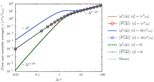
Figure 1: Ensemble and time averaged MSDs for free FLE motion with different initial velocities $v_{0}$. The solid lines represent the theoretical results, Eqs. (9) and (20). The equilibrium MSD and the time averaged MSDs coincide. The ensemble averages for the non-equilibrium processes approach the time averages at long times $\Delta$. All simulations were performed with $h=0.01$ (See Appendix A), $H=0.625$, $t_{a}=0$, and $T/\tau=100$. Ensemble averages contain 1,000 trajectories.

III Free fractional Langevin equation motion and ageing behavior

In this and the following Sections we present the solutions for the ensemble and time averaged MSDs of the FLE and FBM processes introduced here and investigate their ageing behavior. Solutions to the FLE share many general properties with FBM on longer time scales but due to their formulation in phase (velocity and position) space have differentiable trajectories deng ; pottier . We find that the ageing of FBM and FLE is significantly different. Remarkably, the ageing of the FLE varies between the cases of free and confined motion.

III.1 Ensemble averaged moments

The free FLE has been widely used in literature, see for example Refs. eric ; hoefling ; goychuk , and an equilibrium solution was provided by Pottier pottier . Here, we extend this solution to non-equilibrium initial conditions $v_{0}$ analogous to Deng and Barkai deng . From the two-point correlator, corresponding to the fluctuation [$\xi(t)$] average of Eq. (3) shown in Appendix B we obtain the second moment

$$\langle y^{2}(t)\rangle = 2\frac{k_{B}\mathcal{T}}{m}t^{2}E_{2H,3}(-\gamma t^{2H})$$ (9)

$$+\left(v_{0}^{2}-\frac{k_{B}\mathcal{T}}{m}\right)t^{2}E^{2}_{2H,2}(-\gamma t^{2H})$$

with $\gamma=\overline{\gamma}\Gamma(2H-1)/m$. The generalized Mittag-Leffler function $E_{\alpha,\beta}$ has the following series expansions bateman

$$E_{\kappa,\rho}(z)=\sum_{n=0}^{\infty}\frac{z^{n}}{\Gamma(\rho+\kappa n)}$$ (10a)

and

$$E_{\kappa,\rho}(z)=-\sum_{n=1}^{\infty}\frac{z^{-n}}{\Gamma(\rho-\kappa n)}$$ (10b)

around $z=0$ and $|z|=\infty$, respectively. The free FLE process thus exhibits a characteristic turnover from ballistic motion

$$\langle y^{2}(t)\rangle\sim v_{0}^{2}t^{2}$$ (11)

to subdiffusion (note that $H>1/2$),

$$\langle y^{2}(t)\rangle\sim\frac{2}{\gamma}\langle v^{2}\rangle_{\mathrm{th}}\frac{t^{2-2H}}{\Gamma(3-2H)},$$ (12)

where the thermal squared velocity is given by $\langle v^{2}\rangle_{\mathrm{th}}=k_{B}\mathcal{T}/m$. With the anomalous diffusion constant $D_{H}=\langle v^{2}\rangle_{\mathrm{th}}/[\gamma\Gamma(3-2H)]$ we rewrite the latter result in the more convenient form

$$\langle y^{2}(t)\rangle\sim 2D_{H}t^{2-2H}.$$ (13)

This result demonstrates that for FLE motion persistent (positively correlated) fractional Gaussian noise effects subdiffusion, in contrast to the case of FBM shown below. Result (9) and the asymptotic behaviors (11) and (12) are shown in Fig. 1, with excellent agreement between theory and stochastic simulations. The turnover between initial ballistic motion and terminal subdiffusion defines the intrinsic time scale $\tau=\gamma^{-1/(2H)}$. Note that in the case of vanishing initial velocity the ballistic motion is replaced by an initial hyperdiffusive regime

$$\langle y^{2}(t)\rangle\sim 2(2H+1)\gamma\langle v^{2}\rangle_{\mathrm{th}}\frac{t^{2+2H}}{\Gamma(3+2H)},$$ (14)

which is also shown in Fig. 1. The possibility of such a superballistic diffusion for Langevin equation models with vanishing initial velocities was reported in Ref. siegle , showing that superballistic diffusion may occur due to the high amount of energy that the particle gains during equilibration. Notably, this effect occurs even for a Brownian particle ($H=1/2$).

According to Eq. (9), the mean squared position of the free FLE process has a non-equilibrium contribution that is proportional to the difference $v_{0}^{2}-\langle v^{2}\rangle_{\mathrm{th}}$ between initial and thermal kinetic energy. This contribution vanishes algebraically at long times, mirroring the equilibration but also the ageing of the process, see below.

The first moment of $y$,

$$\langle y(t)\rangle=v_{0}tE_{2H,2}(-\gamma t^{2H}),$$ (15)

has the asymptotic behavior

$$\langle y(t)\rangle\sim v_{0}t$$ (16)

at short times and, terminally,

$$\langle y(t)\rangle\sim\frac{v_{0}}{\gamma\Gamma(2-2H)}t^{1-2H}.$$ (17)

It thus approaches zero at long times since the equilibrated process is symmetric. Intriguingly, the approach to the steady state becomes slower when the Hurst parameter tends to 1/2. The Brownian case $H=1/2$ itself equilibrates exponentially, and at long times has the thermal first moment of $\lim_{t\to\infty}\langle y(t)\rangle=v_{0}/\gamma$. This property can be interpreted as follows: the Brownian particle starting with an initial velocity will keep this velocity for a while until the friction slows it down on the characteristic length scale $v_{0}/\gamma$. Afterwards, the particle diffuses symmetrically around this stalling point. A free FLE particle with its coupled power-law forms of the noise correlations and the friction kernel does not feature this property and will on long time scales diffuse around the original starting point.

Combining the second and first moments we obtain the variance $\langle y^{2}(t)\rangle-\langle y(t)\rangle^{2}$. At short times, this quantity is independent of the initial velocity $v_{0}$ and exhibits precisely the hyperdiffusive behavior (14). At longer times, due to the thermalization of the velocity, the asymptotic behavior of $\langle[\Delta y(t)]^{2}\rangle$ follows expression (13).

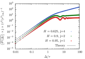
An additional feature of the FLE process are distinct oscillations in the MSD, as shown in Fig. 2. These were reported before jeon1 ; elistas and appear for large Hurst index, and they occur for all possible initial conditions in both the ensemble and time averaged MSD. For which values of the Hurst parameter $H$ are these oscillations possible? The derivative of Eq. (9) shows that the equilibrium MSD of the fee FLE only has extrema and thus oscillates if the function $E_{2H,2}(-\gamma t^{2H})$ has zeros. Numerical analysis demonstrates that this condition is met for $H\gtrsim 0.8\pm 10^{-4}$. Remarkably, this critical Hurst parameter for oscillations is preserved under non-equilibrium initial conditions.

Figure 2: For large Hurst parameters, $H>0.8$, oscillations occur in the MSD of the free FLE. These oscillations are more pronounced for larger $H$. The data was simulated for different Hurst parameters with initial velocities $v_{0}^{2}=\langle v^{2}\rangle_{\mathrm{th}}$, $h=0.01$ (see Appendix A), $T/\tau=100$, and for 1,000 trajectories. The theoretical values are calculated according to Eq. (20). For better visibility, the plots are shifted by the factor j along the logarithmic ordinate.

III.2 Time averaged mean squared displacement and ageing

From the exact results for the second moment $\langle y^{2}(t)\rangle$ and the autocorrelation function $\langle y(t_{1})y(t_{2})\rangle$ we obtain the time averaged MSD through

$$\left<\overline{\delta^{2}(\Delta)}\right> = \frac{1}{T-\Delta}\int_{t_{a}}^{t_{a}+T-\Delta}\Big{(}\langle x^{2}(t^{\prime}+\Delta)\rangle+\langle x^{2}(t^{\prime})\rangle$$ (18)

$$-2\langle x(t^{\prime}+\Delta)x(t^{\prime})\rangle\Big{)}dt^{\prime}.$$

Based on the full solution (70a) for the free FLE, we find that $\langle\overline{\delta^{2}(\Delta)}\rangle$ splits up into two additive contributions,

$$\left<\overline{\delta^{2}(\Delta)}\right>=f_{\mathrm{st}}(\Delta)+f_{\mathrm{age}}(\Delta;t_{a},T).$$ (19)

In contrast to CTRW subdiffusion the time averaged MSD of the free FLE motion does not vanish for long measurement and ageing times, $T$ and $t_{a}$. Namely, it has a stationary contribution $f_{\mathrm{st}}$, that only depends on the lag time $\Delta$. All dependencies on $t_{a}$ or $T$ are captured by the ageing term $f_{\mathrm{age}}$, which decays for long $T$ and $t_{a}$. We will obtain an analogous behavior for the FLE in an harmonic potential and FBM below.

The stationary contribution for the free FLE becomes

$$f_{\mathrm{st}}=2\langle v^{2}\rangle_{\mathrm{th}}\Delta^{2}E_{2H,3}(-\gamma\Delta^{2H}),$$ (20)

with a turnover from the ballistic short time expansion

$$f_{\mathrm{st}}\sim\frac{2\langle v^{2}\rangle_{\mathrm{th}}}{\Gamma(2H)}\Delta^{2}$$ (21)

to the asymptotic subdiffusive form

$$f_{\mathrm{st}}\sim\frac{2\langle v^{2}\rangle_{\mathrm{th}}}{\gamma\Gamma(2H-2)}\Delta^{2-2H}.$$ (22)

For the ageing term the following expression holds,

$$f_{\mathrm{age}} = \frac{v_{0}^{2}-\langle v^{2}\rangle_{\mathrm{th}}}{T-\Delta}\int\limits_{t_{a}}^{t_{a}+T-\Delta}\Big{[}(t+\Delta)E_{2H,2}(-\gamma(t+\Delta)^{2H})$$ (23)

$$\hskip 91.04872pt-tE_{2H,2}(-\gamma t^{2H})\Big{]}^{2}dt,$$

which vanishes, when the initial velocity has the value of the thermal velocity, $\pm\langle v^{2}\rangle_{\mathrm{th}}^{1/2}$. The term in the integral is always positive and at long $t$ has the asymptotic form

$$\Big{[}\ldots\Big{]}^{2}\sim\frac{\Delta^{2}}{\gamma^{2}\Gamma^{2}(1-2H)}t^{-4H},$$ (24)

such that due to $H>1/2$ it is integrable. We can further approximate the ageing term in the experimentally relevant regime. For evaluating time averages it is crucial to have sufficiently long time series, i.e. the collected data should be extensive enough to produce reliable statistics. That means, we will observe the limit $T\gg\Delta$. Additionally, we assume the intrinsic time scale to be very short in comparison to accessible measurement times, i.e. we take the limit $T\gg\tau$. Finally, we keep the ageing time finite, i.e. $T\gg t_{a}$. In these limits, the integral will approach a finite value, $\daleth_{\infty}(\Delta,t_{a})$, due to the above convergence criterion. We thus identify the long-$T$ dependence

$$f_{\mathrm{age}}=\left[v_{0}^{2}-\langle v^{2}\rangle_{\mathrm{th}}\right]\frac{\daleth_{\infty}(\Delta,t_{a})}{T}+\mathcal{O}\left(\gamma^{-2}T^{-4H}\right).$$ (25)

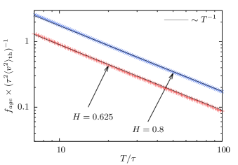
The $1/T$-scaling of the ageing contribution $f_{\mathrm{age}}$ is demonstrated in comparison with simulations results in Fig. 3. For $T\to\infty$ only the stationary term of $\langle\overline{\delta^{2}(\Delta)}\rangle$ remains, and in that limit we find the ergodic behavior

$$\left<\overline{\delta^{2}(\Delta)}\right> = \lim_{t\to\infty}\left<\left[y(t+\Delta)-y(t)\right]^{2}\right>$$ (26)

$$= \left<y^{2}(\Delta)\right>,$$

under the condition that the initial velocity is thermalized, $v_{0}^{2}=\langle v^{2}\rangle_{\mathrm{th}}$, consistent with the results of Ref. deng .

Figure 3: Measurement time $T$ dependence of the free FLE, confirming the proportionality to $1/T$. $f_{\mathrm{age}}$ was calculated by subtracting the theoretical results for $f_{\mathrm{st}}$ (20) from the simulated values for the time averaged MSD. The simulations were run with $h=0.01$ (see Appendix A), $v_{0}^{2}=100\langle v^{2}\rangle_{\mathrm{th}}$, $\Delta/\tau=0.5$, and $t_{a}=0$, and were averaged over 1,000 trajectories.

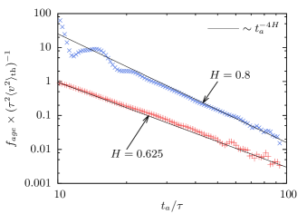
Figure 4: Ageing time dependence of the free FLE motion, recovering the proportionality to $t_{a}^{-4H}$. Parameters: $h=0.01$ (See Appendix A), $\Delta/\tau=0.5$, and $T/\tau=5$, so that the data are in the limit $t_{a}\gg T\gg\Delta$. For $H=0.625$, the initial velocity is $v_{0}^{2}=4\times 10^{4}\langle v^{2}\rangle_{\mathrm{th}}$ and the number of trajectories is 10,000. For $H=0.8$, the initial velocity is $v_{0}^{2}=25\times 10^{4}\langle v^{2}\rangle_{\mathrm{th}}$ and the number of trajectories is $10^{5}$. The simulated values for $H=0.8$ were multiplied by a constant factor of 10 for visual convenience.

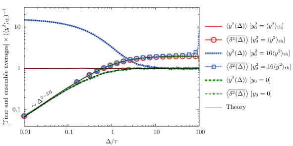
Figure 5: Ensemble averaged and time averaged MSDs for the overdamped FLE motion in a confining, external harmonic potential for $H=0.625$. The simulations were performed with the parameter values $t_{a}=0$, $T/\tau=100$, and $h=0.01$ (see Appendix A), and averaged over $10^{4}$ trajectories. The theoretical behavior is provided by Eqs. (31) and (38). We observe excellent agreement between theory and simulation. In accordance with Ref. jeon1 , the time averages approach twice the value of the ensemble averages.

What happens when the process is strongly aged? In the associated limit of $t_{a}\gg\Delta$ and $t_{a}\gg\gamma^{-1/(2H)}$ as well as $T\gg\Delta$ we obtain

$$f_{\mathrm{age}}=\frac{\left(v_{0}^{2}-\langle v^{2}\rangle_{\mathrm{th}}\right)\Delta^{2}}{(1-4H)\gamma^{2}\Gamma^{2}(1-2H)}\frac{(T+t_{a})^{1-4H}-t_{a}^{1-4H}}{T}.$$ (27)

If additionally $t_{a}\gg T$, we thus find the scaling

$$f_{\mathrm{age}}\sim\frac{\left(v_{0}^{2}-\langle v^{2}\rangle_{\mathrm{th}}\right)\Delta^{2}}{\gamma^{2}\Gamma^{2}(1-2H)}t_{a}^{-4H}.$$ (28)

This asymptotic dependence on the ageing time $t_{a}$ is illustrated in Fig. 4. Above results show that the relaxation of the ageing dependence becomes slower when $H$ approaches the Brownian value $H=1/2$.

Remarkably, the first order correction for highly aged systems is quadratic in the lag time $\Delta$. Hence, the coefficient for the ballistic regime in Eq. (20) could potentially be over- or underestimated if it is gained from aged particle trajectories.

IV Confined fractional Langevin equation motion and ageing behavior

We now turn to the FLE (6) in the presence of a confining, external harmonic potential and analyze the dynamics in terms of the ensemble and time averaged MSDs. In particular, we find the remarkable result that the ageing behavior is different from the free FLE motion.

IV.1 Ensemble averaged moments

In the underdamped case [i.e., keeping the inertial term on the left hand side of Eq. (6)], the second moment of the position can be written in the form (compare Appendix B)

$$\langle y^{2}(t)\rangle = \langle y^{2}\rangle_{\mathrm{th}}+\left(y_{0}^{2}-\langle y^{2}\rangle_{\mathrm{th}}\right)A^{2}(t)$$ (29)

$$+\left(v_{0}^{2}-\langle v^{2}\rangle_{\mathrm{th}}\right)B^{2}(t)+2y_{0}v_{0}A(t)B(t)$$

where $\langle y^{2}\rangle_{\mathrm{th}}=k_{B}\mathcal{T}/\lambda$ is the thermal value of the position coordinate, and $A(t)$ and $B(t)$ are defined via their Laplace transforms ($s$ denoting the Laplace variable) through

$$A(s) =\frac{\displaystyle\gamma s^{1-2H}+ms}{\displaystyle ms^{2}+\gamma s^{2-2H}+\lambda}$$ (30a)

$$B(s) =\frac{\displaystyle m}{\displaystyle ms^{2}+\gamma s^{2-2H}+\lambda}.$$ (30b)

In the overdamped case, which was discussed in Ref. kou , we obtain the simpler result

$$\langle y^{2}(t)\rangle=\langle y^{2}\rangle_{\mathrm{th}}+\left(y_{0}^{2}-\langle y^{2}\rangle_{\mathrm{th}}\right)E_{2-2H}^{2}\left(-\frac{\lambda}{\gamma}t^{2-2H}\right)$$ (31)

with $\gamma=\overline{\gamma}\Gamma(2H-1)$. Here $E_{\alpha}=E_{\alpha,1}$ is the regular Mittag-Leffler function. At short times we observe the leading order behavior

$$\langle y^{2}(t)\rangle\sim y_{0}^{2}-\frac{2\lambda\left(y_{0}^{2}-\langle y^{2}\rangle_{\mathrm{th}}\right)}{\gamma\Gamma(3-2H)}t^{2-2H}.$$ (32)

That is, starting from the initial value $y_{0}^{2}$ we have a decay or increase of $\langle y^{2}(t)\rangle$ depending on the sign of $y_{0}^{2}-\langle y^{2}\rangle_{\mathrm{th}}$. Asymptotically the second moment exhibits the power-law convergence

$$\langle y^{2}(t)\rangle\sim\langle y^{2}\rangle_{\mathrm{th}}+\left(y_{0}^{2}-\langle y^{2}\rangle_{\mathrm{th}}\right)\frac{\gamma^{2}}{\lambda^{2}}\frac{t^{4H-4}}{\Gamma^{2}(2H-1)}$$ (33)

to the thermal value $\langle y^{2}\rangle_{\mathrm{th}}=k_{B}\mathcal{T}/\lambda$. The approach to this thermal value is from above when $y_{0}^{2}>\langle y^{2}\rangle_{\mathrm{th}}$ and from below in the opposite case. This relaxation occurs on the intrinsic time scale $\tau=(\gamma/\lambda)^{1/(2-2H)}$. The above behavior is shown in Fig. 5. We note that in terms of dimensionless variables Eq. (29) has two free parameters: the rescaled initial velocity and the initial position. In the overdamped case only the initial position is relevant, see also the full solutions, Eqs. (70b) and (70c).

The first moment of the confined FLE motion is given by the relaxation pattern

$$\langle y(t)\rangle=A(t)y_{0}+B(t)v_{0}$$ (34)

for the full solution and, in the overdamped case, by the Mittag-Leffler form

$$\langle y(t)\rangle=y_{0}E_{2-2H}\left(-\frac{\lambda}{\gamma}t^{2-2H}\right)$$ (35)

with the asymptotic behavior

$$\langle y(t)\rangle\sim\frac{y_{0}\gamma}{\gamma\Gamma(2H-1)}t^{2H-2}.$$ (36)

IV.2 Time averaged mean squared displacement and ageing

The full solution for the time averaged MSD $\langle\overline{\delta^{2}(\Delta)}\rangle$ is additive as in Eq. (19) with the following two contributions. The stationary term reads

$$f_{\mathrm{st}}=2\langle y^{2}\rangle_{\mathrm{th}}(1-A(\Delta))$$ (37)

in the underdamped case and

$$f_{\mathrm{st}}=2\langle y^{2}\rangle_{\mathrm{th}}\left[1-E_{2-2H}\left(-\frac{\lambda}{\gamma}\Delta^{2-2H}\right)\right]$$ (38)

in the overdamped case. The latter turns over from the subdiffusive short lag time growth

$$f_{\mathrm{st}}\sim 2\langle y^{2}\rangle_{\mathrm{th}}\frac{\lambda}{\gamma}\frac{\Delta^{2-2H}}{\Gamma(3-2H)}$$ (39)

to the asymptotic long-$\Delta$ approach

$$f_{\mathrm{st}}\sim 2\langle y^{2}\rangle_{\mathrm{th}}\left[1-\frac{\gamma}{\lambda}\frac{\Delta^{2H-2}}{\Gamma(2H-1)}\right]$$ (40)

to twice the thermal value $\langle y^{2}\rangle_{\mathrm{th}}$. This factor of two stems from the very definition of the time averaged MSD (1), compare Eq. (18). jeon1 .

The ageing term becomes

$$f_{\mathrm{age}} = \frac{y_{0}^{2}-\langle y^{2}\rangle_{\mathrm{th}}}{T-\Delta}\int\limits_{t_{a}}^{t_{a}+T-\Delta}\Big{(}A(t+\Delta)-A(t)\Big{)}^{2}dt$$ (41)

$$+\frac{v_{0}^{2}-\langle v^{2}\rangle_{\mathrm{th}}}{T-\Delta}\int\limits_{t_{a}}^{t_{a}+T-\Delta}\Big{(}B(t+\Delta)-B(t)\Big{)}^{2}dt$$

$$+\frac{2y_{0}v_{0}}{T-\Delta}\int\limits_{t_{a}}^{t_{a}+T-\Delta}\Big{(}A(t+\Delta)-A(t)\Big{)}$$

$$\hskip 68.28644pt\times\Big{(}B(t+\Delta)-B(t)\Big{)}dt,$$

which can be used for numerical evaluation. In the overdamped case, this expression simplifies to

$$f_{\mathrm{age}} = \frac{y_{0}^{2}-\langle y^{2}\rangle_{\mathrm{th}}}{T-\Delta}\int\limits_{t_{a}}^{t_{a}+T-\Delta}\left[E_{2-2H}\left(-\frac{\lambda}{\gamma}(t+\Delta)^{2-2H}\right)\right.$$ (42)

$$\hskip 68.28644pt\left.-E_{2-2H}\left(-\frac{\lambda}{\gamma}t^{2-2H}\right)\right]^{2}dt$$

For $t\gg\Delta$ the integrand in the above expression decays like

$$\Big{[}\ldots\Big{]}^{2} \sim \frac{\lambda^{2}}{\gamma^{2}}\Delta^{2}t^{2-4H}E_{2-2H,2-2H}^{2}\left(-\frac{\lambda}{\gamma}t^{2-2H}\right)$$ (43)

$$\sim \frac{\gamma^{2}}{\lambda^{2}\Gamma^{2}(2-2H)}\Delta^{2}t^{4H-6},$$

where the second approximation holds when, in addition, $t\gg\tau$. As the exponent $4H-6$ ranges in the interval between $-2$ and $-4$ the integral converges and approaches the finite value $\daleth^{\prime}_{\infty}(\Delta,t_{a})$, which increases with $t_{a}$. For $T\gg\Delta,\tau,t_{a}$ we thus find

$$f_{\mathrm{age}}\sim\left(y_{0}^{2}-\langle y^{2}\rangle_{\mathrm{th}}\right)\frac{\daleth^{\prime}_{\infty}(\Delta,t_{a})}{T}.$$ (44)

This $1/T$ dependence on the process time $T$ is in good agreement with our simulations, as demonstrated in Fig. 6.

Figure 6: Measurement time $T$ dependence of the overdamped confined FLE process showing the predicted $T^{-1}$ decay. $f_{\mathrm{age}}$ was obtained by subtracting the theoretical value of $f_{\mathrm{st}}$ from the time averaged MSD. The simulation were performed for $y_{0}^{2}=16\langle y^{2}\rangle_{\mathrm{th}}$, $h=0.01$ (see Appendix A), $\Delta/\tau=0.3$, and $t_{a}=0$, and were averaged over $10^{4}$ trajectories.

In the ageing limit $t_{a}\gg\Delta$, $t_{a}\gg\tau$, and $T\gg\Delta$ we find the asymptotic behavior

$$f_{\mathrm{age}}\sim\frac{(y_{0}^{2}-\langle y^{2}\rangle_{\mathrm{th}})\gamma^{2}}{(4H-5)\lambda^{2}\Gamma^{2}(2-2H)}\Delta^{2}\frac{(T+t_{a})^{4H-5}-t_{a}^{4H-5}}{T}.$$ (45)

If we assume strong ageing in the sense $t_{a}\gg T$, we arrive at the scaling behavior

$$f_{\mathrm{age}}\sim\frac{(y_{0}^{2}-\langle y^{2}\rangle_{\mathrm{th}})\gamma^{2}}{\lambda^{2}\Gamma^{2}(2-2H)}\Delta^{2}t_{a}^{4H-6}.$$ (46)

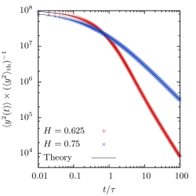
This prediction is confirmed in Fig. 7. Note the difference to the $t_{a}$-scaling (28) of the free FLE motion. Remarkably, the ageing terms for over- and underdamped FLE under confinement coincide in the considered limits.

Figure 7: Left: ageing dependence on $t_{a}$ of the overdamped confined FLE process. The simulations used $y_{0}^{2}=10^{8}\langle y^{2}\rangle_{\mathrm{th}}$ and $h=0.01$ (see Appendix A), and the values are averaged over $10^{4}$ trajectories. We chose $\Delta/\tau=0.3$ and $T/\tau=0.4$ to guarantee the limit $t_{a}\gg\Delta,T$. In order to validate that the linearization in the simulation scheme is accurate for this particular $h$ and the comparatively high starting kinetic energies, the mean squared position is plotted on the right side and compared to the theoretical result (31), observing excellent agreement.

V Fractional Brownian motion

We now turn to FBM, in which the fractional Gaussian noise is external. Therefore, when we consider the ensemble averaged MSD of free FBM,

$$\langle x^{2}(t)\rangle=2D_{H}t^{2H},$$ (47)

we see that antipersistent noise with $0<H<1/2$ corresponds to subdiffusion, in contrast to FLE motion, where the noise is counterweighted by the friction kernel. Here, we calculate the dynamic quantities for confined FBM described by Eq. (8). This derivation is analogous to Ref. jeon1 .

V.1 Ensemble averaged moments

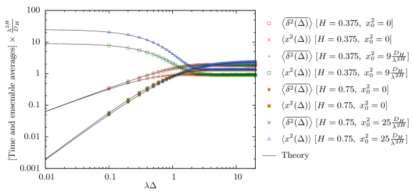
Figure 8: Time and ensemble averaged MSDs, Eqs. (55) and (48) for confined FBM with the indicated parameters. We observe excellent agreement between theory and simulation. For a fixed Hurst parameter, the time averaged MSD approaches twice the stationary value $\langle x^{2}\rangle_{\mathrm{th}}$. The stationary values depend on the Hurst parameter $H$, see Ref. oleksii . The short time behavior depends on the initial value $x_{0}$. All simulations were run with $h=0.1$ (see Appendix A), $T/\tau=300$, and $t_{a}=0$, and represent averages over $10^{5}$ trajectories.

As this process does not fulfill Kubo’s fluctuation dissipation theorem, it does not have a solution that starts in equilibrium. If one extends the solution of Ref. jeon1 to non-zero initial conditions one obtains the second moments listed in Appendix B. The ensemble averaged MSD yields,

$$\langle x^{2}(t)\rangle = x_{0}^{2}e^{-2\lambda t}+\frac{D_{H}}{\lambda^{2H}}\gamma(2H+1,\lambda t)+2D_{H}e^{-\lambda t}t^{2H}$$ (48)

$$-\frac{\lambda D_{H}}{2H+1}e^{-2\lambda t}t^{2H+1}M(2H+1,2H+2,\lambda t).$$

Here, $\gamma$ is the lower incomplete $\gamma$-function, and $M$ denotes the Kummer function abramowitz . FBM in an harmonic external potential has an intrinsic time scale of $\tau=1/\lambda$, see Fig. 8. Rescaling of the dynamic equation for the confined FBM reveals that the only free parameter of this equation is the initial position.

At short times we obtain the behavior

$$\langle x^{2}(t)\rangle\sim x_{0}^{2}-2\lambda x_{0}^{2}t+2D_{H}t^{2H}.$$ (49)

For the case $H<1/2$ the fractional term dominates, for $H>1/2$ the linear term dominates. Counterintuitively, the process exhibits overshooting, i.e. local maxima in the MSD, for the subdiffusive case $H<1/2$ (not shown). In the limit $\lambda=0$ we recover the ensemble averaged MSD (47) of free FBM. With the asymptotic expansions

$$M(2H+1,2H+2,z)\sim\frac{2H+1}{z}e^{z}$$ (50)

and

$$\gamma(2H+1,z)\sim\Gamma(2H+1)-z^{2H}e^{-z}$$ (51)

for the Kummer and incomplete $\gamma$-functions, respectively, in the limit $t\gg\tau$ we find

$$\langle x^{2}(t)\rangle \sim \frac{D_{H}\Gamma(2H+1)}{\lambda^{2H}}+x_{0}^{2}e^{-2\lambda t}$$ (52)

$$-\frac{2}{\lambda^{2}}2H(2H-1)D_{H}t^{2H-2}e^{-\lambda t}.$$

Thus, after an exponential relaxation with characteristic decay time $1/\lambda$ the system reaches the stationary value

$$\langle x^{2}\rangle_{\mathrm{st}}=D_{H}\Gamma(2H+1)/\lambda^{2H}.$$ (53)

As the Kubo condition is missing for this process, the stationary value explicitly depends on the Hurst parameter $H$, thus demonstrating the non-equilibrium character. The activation as function of $H$ of the stationary value $\langle x^{2}\rangle_{\mathrm{st}}$ was demonstrated by simulations in Ref. oleksii . For the first moment we find the exponential decay

$$\langle x(t)\rangle=x_{0}e^{-\lambda t}.$$ (54)

V.2 Time averaged mean squared displacement and ageing

From the explicit result for the time averaged MSD $\langle\overline{\delta^{2}(\Delta)}\rangle$ in Eq. (71) we see that also for this process we obtain the additive combination (19) of a stationary and an ageing contribution. The stationary part is given by

$$f_{\mathrm{st}} = 2D_{H}\Delta^{2H}+\frac{2D_{H}}{\lambda^{2H}}\Gamma(2H+1)$$ (55)

$$-\frac{D_{H}}{\lambda^{2H}}(\Gamma(2H+1,\lambda\Delta)e^{\lambda\Delta}+\Gamma(2H+1)e^{-\lambda\Delta})$$

$$-\frac{D_{H}\lambda}{2H+1}\Delta^{2H+1}e^{-\lambda\Delta}M(2H+1;2H+2;\lambda\Delta),$$

where $\Gamma(a,z)$ is the upper incomplete $\Gamma$-function. Interestingly, as discovered in Ref. jeon1 the approach to the stationary value of the time averaged MSD is of power-law form,

$$f_{\mathrm{st}} \sim \frac{2D_{H}\Gamma(2H+1)}{\lambda^{2H}}-\frac{D_{H}}{\lambda^{2H}}\Gamma(2H+1)e^{-\lambda\Delta}$$ (56)

$$+\frac{4H(2H-1)D_{H}}{\lambda^{2}}\Delta^{2H-2},$$

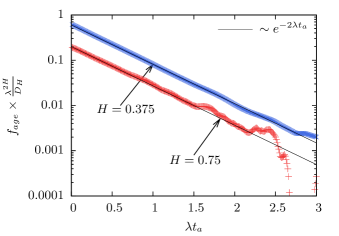
contrasting the exponentially fast relaxation of the ensemble MSD. Note again the factor of two in the stationary value due to the definition of $\langle\overline{\delta^{2}(\Delta)}\rangle$. We demonstrate in Figs. 9 and 10 that the measurement time dependence of the ageing term is indeed of the form $f_{\mathrm{age}}\simeq 1/T$, and that the ageing time dependence is of the form

$$f_{\mathrm{age}}\sim x_{0}^{2}\exp(-2\lambda t_{a}).$$ (57)

Both relations can be shown analytically.

Figure 9: Measurement time $T$ dependence for confined FBM, confirming the $1/T$ behavior. Simulation parameters: $h=0.01$ (see Appendix A), $\Delta/\tau=0.2$, and $t_{a}=0$. The results were averaged over $10^{5}$ trajectories. The simulation for $H=0.75$ started with $x_{0}^{2}=25D_{H}/\lambda^{2H}$, the one for $H=0.375$ with $x_{0}^{2}=9D_{H}/\lambda^{2H}$.

Figure 10: Ageing for confined FBM, showing the predicted exponential decay (57). Simulations used $h=0.01$ (see Appendix A) and $\Delta/\tau=0.2$, averaging over $10^{5}$ trajectories. The simulation for $H=0.75$ started with $x_{0}^{2}=25D_{H}/\lambda^{2H}$, the one for $H=0.375$ with $x_{0}^{2}=9D_{H}/\lambda^{2H}$.

VI Discussion

We studied the FLE and FBM models for anomalous diffusion which are driven by fractional Gaussian noise. From results for the ensemble averaged first and second moments, we obtained the associated time averaged MSD $\langle\overline{\delta^{2}(\Delta)}\rangle$. The exact expression for $\langle\overline{\delta^{2}(\Delta)}\rangle$ was shown to separate into two additive contributions, a stationary one and an ageing term. The ageing term vanishes at large measurement times inverse-proportionally. While solutions to regular Langevin equations with white noise as well as the confined FBM show exponential relaxation of the time averaged MSD in the ageing time, solutions to FLEs exhibit power-law relaxation and power-law ageing with a characteristic exponent between -1 and -3. Notably, the ageing exponents differ between free and confined FLE motion.

The existence of the finite stationary term of the time averaged MSD for stochastic processes driven by fractional Gaussian noise contrasts the properties of the CTRW process, for which the time averaged MSD decays to zero in the respective limits. The origin of this difference is that a CTRW particle effectively grinds to a complete halt after a sufficiently long time while a free FLE particle keeps spreading. Hence, the ageing dynamics in CTRWs and the free FLE are well distinguishable. In particular, it should be noted that free FBM, which is equivalent to overdamped free FLE motion deng does not exhibit ageing at all.

What happens when, instead of fixed initial conditions $v_{0}$, $x_{0}$, and $y_{0}$ as well as ageing times $t_{a}$ we analyze an ensemble of trajectories with distributed ageing times or initial conditions? In such cases our ageing formulas may also be useful. Consider the example of free FLE motion. Let $\langle\cdot\rangle$ denote the ensemble average for a fixed ageing time $t_{a}$ and a fixed initial condition $v_{0}$. Let $\langle\cdot\rangle_{\mathrm{dis}}$ denote the ensemble average over trajectories with distributed ageing times $t_{a}$ and initial velocities $v_{0}$, and let $P$ denote the probability for a given value of $v_{0}$ and $t_{a}$. Then we obtain

$$\left<\overline{\delta^{2}(\Delta)}\right>_{\mathrm{dis}}=\int\limits_{0}^{\infty}dt_{a}\int\limits_{-\infty}^{\infty}dv_{0}\left<\overline{\delta^{2}(\Delta;t_{a},v_{0})}\right>P(t_{a},v_{0})$$ (58)

Hence, the time averaged MSD over an ensemble of trajectories with distributed initial conditions and ageing times can be calculated by weighting our result for the time averaged MSD for fixed $t_{a}$ and $v_{0}$ with the probability for that ageing time and initial condition to occur, $P(t_{a},v_{0})$. This probability will eventually depend on the experimental setup.

Appendix A Simulation Schemes

The simulation schemes for the stochastic differential equations are based on the method originally proposed by Deng and Barkai deng and also used in Ref. jae . In order to derive the scheme, we first integrate the dynamic equations (3), (6), and (8) over time. This leads to

$$mv(t)=mv_{0}-\frac{\overline{\gamma}}{2H-1}\int\limits_{0}^{t}(t-\tau)^{2H-1}v(\tau)d\tau+\eta B_{H}(t)$$ (59)

for the free FLE,

$$\lambda\int\limits_{0}^{t}y(\tau)d\tau = -\overline{\gamma}\int\limits_{0}^{t}(t-\tau)^{2H-2}y(\tau)d\tau$$ (60)

$$+\frac{\overline{\gamma}y_{0}}{2H-1}t^{2H-1}+\eta B_{H}(t)$$

for the overdamped confined FLE, and

$$x(t)=x_{0}-\lambda\int\limits_{0}^{t}x(\tau)d\tau+B_{H}(t).$$ (61)

for confined FBM. These integrals are interpreted trajectory-wise, in analogy to Refs. mandelbrot ; gripenberg ; kou . We then rescale these equations according to $y\to y/\sqrt{k_{B}\mathcal{T}/(m\gamma^{1/(2H)})}$ (free FLE motion), $y\to y/\sqrt{k_{B}\mathcal{T}/\lambda}$ (confined FLE motion) and $x\to x/\sqrt{D_{H}/\lambda^{2H}}$ (confined FBM). The time is rescaled through $t\to t/\tau$, where $\tau$ is the intrinsic time scale of each process. FBM is rescaled by $B_{H}\to(\tau)^{-H}B_{H}$. Dividing the interval $[0,t]$ into $n+1$ intervals of even length $h$, we linearize the fractional derivatives using the results from Diethelm et al. diethelm

$$\int\limits_{0}^{t_{n+1}}(t_{n+1}-\tau)^{\alpha-1}f(\tau)d\tau\approx\frac{h^{\alpha}}{\alpha(\alpha+1)}\sum_{j=0}^{n+1}a_{j,n+1}f(t_{j})$$ (62)

where

$$a_{j,n+1}=\left\{\begin{array}[]{ll}n^{\alpha+1}-(n-\alpha)(n+1)^{\alpha},&j=0\\[5.69046pt] (n-j+2)^{\alpha+1}+(n-j)^{\alpha+1}-2(n-j+1)^{\alpha+1},&1\leq j\leq n\\[5.69046pt] 1,&j=n+1.\end{array}\right.$$ (63)

One can then solve for the $v(t_{n+1})$, $y(t_{n+1})$, and $x(t_{n+1})$. This leads in the case of the free FLE to

$$v(t_{n+1})=\frac{\Gamma(2H+2)}{C}v_{0}-\frac{h^{2H}}{C}\sum_{j=0}^{n}a_{j,n+1}v(t_{j})+\frac{\Gamma(2H+2)}{C\sqrt{\Gamma(2H+1)D_{H}}}B_{H}(t_{n+1})$$ (64)

with $C=\Gamma(2H+2)+h^{2H}$ and

$$a_{j,n+1}=\left\{\begin{array}[]{ll}n^{2H+1}-(n-2H)(n+1)^{2H},&j=0\\[5.69046pt] (n-j+2)^{2H+1}+(n-j)^{2H+1}-2(n-j+1)^{2H+1},&1\leq j\leq n\\[5.69046pt] 1&j=n+1\end{array}\right..$$ (65)

The velocities obtained by this scheme can then be integrated by the trapezoidal rule to obtain the particle position. For the overdamped FLE-$\lambda$ we get

$$y(t_{n+1})=-\sum_{j=0}^{n}d_{n+1,j}y(t_{j})+\frac{2y_{0}}{\frac{1}{H}+\Gamma(2H)h^{2-2H}}(n+1)^{2H-1}+\frac{2}{\sqrt{D_{H}\Gamma(2H+1)}\left(h+\frac{2h^{2H-1}}{\Gamma(2H+1)}\right)}B_{H}(t_{n+1})$$ (66)

with

$$d_{n+1,j}=\left\{\begin{array}[]{ll}\frac{1}{1+\frac{2h^{2H-2}}{\Gamma(2H+1)}}+\frac{2}{2+\Gamma(2H+1)h^{2-2H}}\left[n^{2H}-(n+1-2H)(n+1)^{2H-1}\right],&j=0\\[17.07182pt] \frac{2}{1+\frac{2h^{2H-2}}{\Gamma(2H+1)}}+\frac{2}{2+\Gamma(2H+1)h^{2-2H}}\left[(n-j+2)^{2H}+(n-j)^{2H}-2(n-j+1)^{2H}\right],&1\leq j\leq n\end{array}\right.$$ (67)

and, finally, in the case of confined FBM one obtains

$$x(t_{n+1})=\frac{2-h}{2+h}x(t_{n})+\frac{2}{(2+h)\sqrt{D_{H}}}(B_{H}(t_{n+1})-B_{H}(t_{n})).$$ (68)

Hence, we derived expressions for the particle positions or velocities at the time point $t_{n+1}$ depending on all prior positions or velocities. These expressions can be used to obtain trajectories of the corresponding stochastic processes. To simulate FBM, the implementation provided in Ref. dieker was used. It is based on a method originally developed by Hosking hosking . It should be noted that all the proposed algorithms have time complexity of order $n^{2}$.

Appendix B Solutions to the stochastic differential equations

To analytically solve equations equations (3), (6), and (8) we formally derive their solutions in Laplace space, treating the noise as a well-behaved function of time analogous to Deng and Barkai deng . Averaging and considering that $\langle\xi(s)\rangle=0$ holds for the Laplace transform of fractional Gaussian noise (2) allows us to identify the first moments (15), (34), (35), and (54). We then multiply each formal solution at two different points in Laplace space. The average of these products gives us the double Laplace transform of the second moments. To obtain explicit expressions, we use the double Laplace transform of fractional Gaussian noise ($\tau$ and $s$ being the Laplace variables)

$$\langle\xi(s)\xi(\tau)\rangle = D_{H}\Gamma(2H+1)\frac{s^{1-2H}+\tau^{1-2H}}{s+\tau}.$$ (69)

The second moments follow as

$$\langle y(t_{1})y(t_{2})\rangle = \frac{k_{B}\mathcal{T}}{m}\Big{\{}t_{1}^{2}E_{2H,3}(-\gamma t_{1}^{2H})+t_{2}^{2}E_{2H,3}(-\gamma t_{2}^{2H})-(t_{1}-t_{2})^{2}E_{2H,3}(-\gamma|t_{1}-t_{2}|^{2H})\Big{\}}$$ (70a)

$$+\left(v_{0}^{2}-\frac{k_{B}\mathcal{T}}{m}\right)t_{1}t_{2}E_{2H,2}(-\gamma t_{1}^{2H})E_{2H,2}(-\gamma t_{2}^{2H})$$

for free FLE motion,

$$\langle y(t_{1})y(t_{2})\rangle = \frac{k_{B}\mathcal{T}}{\lambda}A(|t_{2}-t_{1}|)+\left(y_{0}^{2}-\frac{k_{B}\mathcal{T}}{\lambda}\right)A(t_{1})A(t_{2})+\left(v_{0}^{2}-\frac{k_{B}\mathcal{T}}{m}\right)B(t_{1})B(t_{2})$$ (70b)

$$+y_{0}v_{0}(A(t_{1})B(t_{2})+A(t_{2})B(t_{1}))$$

for confined FLE motion [compare Eqs. (30)],

$$\langle y(t_{1})y(t_{2})\rangle=\frac{k_{B}\mathcal{T}}{\lambda}E_{2-2H}(-\frac{\lambda}{\gamma}|t_{2}-t_{1}|^{2-2H})+\left(y_{0}^{2}-\frac{k_{B}\mathcal{T}}{\lambda}\right)E_{2-2H}(-\frac{\lambda}{\gamma}t_{1}^{2-2H})E_{2-2H}(-\frac{\lambda}{\gamma}t_{2}^{2-2H})$$ (70c)

for overdamped confined FLE motion (note that the definitions of $$\gamma$$ differ for confined and free FLE motion), and

$$\langle x(t_{1})x(t_{2})\rangle = D_{H}\{e^{-\lambda t_{1}}t_{2}^{2H}+e^{-\lambda t_{2}}t_{1}^{2H}-|t_{1}-t_{2}|^{2H}\}+\frac{D_{H}}{2\lambda^{2H}}\{e^{-\lambda|t_{2}-t_{1}|}\gamma(2H+1,\lambda t_{1})+e^{\lambda|t_{2}-t_{1}|}\gamma(2H+1,\lambda t_{2})\}$$ (70d)

$$-\frac{D_{H}}{2\lambda^{2H}}e^{\lambda|t_{2}-t_{1}|}\gamma(2H+1,\lambda|t_{2}-t_{1}|)-\frac{\lambda D_{H}}{2(2H+1)}e^{-\lambda(t_{2}+t_{1})}t_{1}^{2H+1}M(2H+1;2H+2;\lambda t_{1})$$

$$-\frac{\lambda D_{H}}{2(2H+1)}e^{-\lambda(t_{2}+t_{1})}t_{2}^{2H+1}M(2H+1;2H+2;\lambda t_{2})$$

$$+\frac{\lambda D_{H}}{2(2H+1)}|t_{2}-t_{1}|^{2H+1}e^{-\lambda|t_{2}-t_{1}|}M(2H+1;2H+2;\lambda|t_{2}-t_{1}|)+x_{0}^{2}e^{-\lambda(t_{1}+t_{2})},~{}(t_{2}>t_{1}).$$

for confined FBM.

Taken together, the first moments (15), (34), (35), and (54) and the second moments (70a) to (70d) compose the full solutions of the stochastic differential equations (3), (6), and (8) vankampen . These solutions provide fundamental insight into the behavior of the underlying processes. They allow one to interpret the short and long time correlations, capture the complete dynamics of the equilibration, and provide the basis to calculate other valuable quantities, such as velocity correlations or the time averaged MSDs.

Appendix C Time averaged MSD for confined FBM

For confined FBM the time averaged MSD takes on the complex form

$$\left<\overline{\delta^{2}(\Delta)}\right>=2D_{H}\Delta^{2H}+\frac{D_{H}}{\lambda^{2H}}e^{\lambda\Delta}\gamma(2H+1,\lambda\Delta)-\frac{D_{H}\lambda}{2H+1}\Delta^{2H+1}e^{-\lambda\Delta}M(2H+1;2H+2;\lambda\Delta)$$ (71)

$$+\frac{x_{0}^{2}}{2\lambda(T-\Delta)}e^{-2\lambda t_{a}}\big{(}1-e^{-2\lambda(T-\Delta)}\big{)}\left\{1+e^{-\lambda\Delta}\left(e^{-\lambda\Delta}-2\right)\right\}$$

$$+(1-e^{-\lambda\Delta})\frac{D_{H}}{(T-\Delta)}\Big{\{}(t_{a}+T-\Delta)^{2H+1}e^{-\lambda(t_{a}+T-\Delta)}-t_{a}^{2H+1}e^{-\lambda t_{a}}\Big{\}}$$

$$+(1-e^{\lambda\Delta})\frac{D_{H}}{(T-\Delta)}\Big{\{}(t_{a}+T)^{2H+1}e^{-\lambda(t_{a}+T)}-(t_{a}+\Delta)^{2H+1}e^{-\lambda(t_{a}+\Delta)}\Big{\}}$$

$$+(1-e^{-\lambda\Delta})\frac{D_{H}}{2(2H+1)(T-\Delta)}\Big{\{}(t_{a}+T-\Delta)^{2H+1}e^{-2\lambda(t_{a}+T-\Delta)}M(2H+1;2H+2,\lambda(t_{a}+T-\Delta))$$

$$\hskip 142.26378pt-t_{a}^{2H+1}e^{-2\lambda t_{a}}M(2H+1;2H+2,\lambda t_{a})\Big{\}}$$

$$+(1-e^{\lambda\Delta})\frac{D_{H}}{2(2H+1)(T-\Delta)}\Big{\{}(t_{a}+T)^{2H+1}e^{-2\lambda(t_{a}+T)}M(2H+1;2H+2,\lambda(t_{a}+T))$$

$$\hskip 142.26378pt-(t_{a}+\Delta)^{2H+1}e^{-2\lambda(t_{a}+\Delta)}M(2H+1;2H+2,\lambda(t_{a}+\Delta))\Big{\}}$$

$$+(1-e^{-\lambda\Delta})\frac{D_{H}}{\lambda^{2H}(T-\Delta)}\Bigg{\{}\gamma(2H+1,\lambda(t_{a}+T-\Delta))\left(t_{a}+T-\Delta-\frac{4H-1}{2\lambda}\right)-\gamma(2H+1,\lambda t_{a})\left(t_{a}-\frac{4H-1}{2\lambda}\right)\Bigg{\}}$$

$$+(1-e^{\lambda\Delta})\frac{D_{H}}{\lambda^{2H}(T-\Delta)}\Bigg{\{}\gamma(2H+1,\lambda(t_{a}+T))\left(t_{a}+T-\frac{4H-1}{2\lambda}\right)-\gamma(2H+1,\lambda(t_{a}+\Delta))\left(t_{a}+\Delta-\frac{4H-1}{2\lambda}\right)\Bigg{\}}.$$

References

• (1) E. Barkai, Y. Garini, and R. Metzler, Phys. Today 65(8), 29 (2012).
• (2) I. M. Sokolov, Soft Matter 8, 9043 (2012).
• (3) J. H. P. Schulz, E. Barkai, and R. Metzler, Phys. Rev. Lett. 110, 020602 (2013).
• (4) Y. He, S. Burov, R. Metzler, and E. Barkai, Phys. Rev. Lett. 101, 058101 (2008).
• (5) S. Burov, J.-H. Jeon, R. Metzler, and E. Barkai, Phys. Chem. Chem. Phys. 13, 1800 (2011).
• (6) E. W. Montroll and G. H. Weiss, J. Math. Phys. 6, 167 (1965); H. Scher and E. W. Montroll, Phys. Rev. B 12, 2455 (1975).
• (7) J.-P. Bouchaud, J. Phys. I (Paris) 2, 1705 (1992); G. Bel and E. Barkai, Phys. Rev. Lett. 94, 240602 (2005); A. Rebenshtok and E. Barkai, ibid. 99, 210601 (2007).
• (8) A. Lubelski, I. M. Sokolov, and J. Klafter, Phys. Rev. Lett. 100, 250602 (2008).
• (9) Defined in terms of the stationary distribution Pst(x)=limtP(x,t)subscript𝑃st𝑥subscript𝑡𝑃𝑥𝑡P_{\mathrm{st}}(x)=\lim_{t\to\infty}P(x,t) as x2th=x2Pst(x)𝑑xsubscriptdelimited-⟨⟩superscript𝑥2thsuperscript𝑥2subscript𝑃st𝑥differential-d𝑥\langle x^{2}\rangle_{\mathrm{th}}=\int x^{2}P_{\mathrm{st}}(x)dx.
• (10) S. Burov, R. Metzler, and E. Barkai, Proc. Natl. Acad. Sci. USA 107, 13228 (2010).
• (11) T. Neusius, I. M. Sokolov, and J. C. Smith, Phys. Rev. E 80, 011109 (2009).
• (12) J.-H. Jeon, V. Tejedor, S. Burov, E. Barkai, C. Selhuber-Unkel, K. Berg-Sørensen, L. Oddershede, and R. Metzler, Phys. Rev. Lett. 106, 048103 (2011).
• (13) A. V. Weigel, B. Simon, M. M. Tamkun, and D. Krapf, Proc. Nat. Acad. Sci. USA 108, 6438 (2011).
• (14) S. M. A. Tabei, S. Burov, H. Y. Kim, A. Kuznetsov, T. Huynh, J. Jureller, L. H. Philipson, A. R. Dinner, and N. F. Scherer, Proc. Natl. Acad. Sci. USA 110, 4911 (2013).
• (15) M. Magdziarz, R. Metzler, W. Szczotka, and P. Zebrowski, Phys. Rev. E 85, 051103 (2012); V. Tejedor and R. Metzler, J. Phys. A 43, 082002 (2010).
• (16) M. A. Lomholt, L. Lizana, R. Metzler, and T. Ambjörnsson, Phys. Rev. Lett. 110, 208301 (2013).
• (17) A. G. Cherstvy, A. V. Chechkin, and R. Metzler, E-print arXiv:1303.5533.
• (18) G. Zumofen and J. Klafter, Physica D 69, 436 (1993); D. Froemberg and E. Barkai, Phys. Rev. E 87, 030104(R) (2013); A. Godec and R. Metzler, Phys. Rev. Lett. 110, 020603 (2013).
• (19) E. Barkai and Y.-C. Cheng, J. Chem. Phys. 118, 6167 (2003); E. Barkai, Phys. Rev. Lett. 90, 104101 (2003).
• (20) W. Deng and E. Barkai, Phys. Rev. E 79, 011112 (2009).
• (21) J.-H. Jeon and R. Metzler, Phys. Rev. E 81, 021103 (2010).
• (22) J.-H. Jeon and R. Metzler, Phys. Rev. E 85, 021147 (2012).
• (23) The additional factor of 2 arises from the definition of the time averaged MSD, compare Eq. (18).
• (24) F. Höfling and T. Franosch, Rep. Prog. Phys. 76, 046602 (2013).
• (25) I. Goychuk, Phys. Rev. E 80, 046125 (2009); Adv. Chem. Phys. 150, 187 (2012).
• (26) J. Szymanski and M. Weiss, Phys. Rev. Lett. 103, 038102 (2009).
• (27) L. P. Sanders and T. Ambjörnsson, J. Chem. Phys. 136, 175103 (2012); L. Lizana, T. Ambjörnsson, A. Taloni, E. Barkai, and M. A. Lomholt, Phys. Rev. E 81, 051118 (2010).
• (28) I. Bronstein, Y. Israel, E. Kepten, S. Mai, Y. Shav-Tal, E. Barkai, and Y. Garini, Phys. Rev. Lett. 103, 018102 (2009); K. Burnecki, E. Kepten, J. Janczura, I. Bronshtein, Y. Garini, and A. Weron, Biophys. J. 103, 1839 (2012).
• (29) S. C. Weber, A. J. Spakowitz, and J. A. Theriot, Phys. Rev. Lett. 104, 238102 (2010).
• (30) J.-H. Jeon, H. Martinez-Seara Monne, M. Javanainen, and R. Metzler, Phys. Rev. Lett. 109, 188103 (2012); G. R. Kneller, K. Baczynski, and M. Pasenkiewicz-Gierula, J. Chem. Phys. 135, 141105 (2011).
• (31) J.-H. Jeon, N. Leijnse, L. Oddershede, and R. Metzler, New J. Phys. 15, 045011 (2013).
• (32) R. Kubo, Rep. Prog. Phys. 29, 255 (1966).
• (33) B. B. Mandelbrot and J. W. van Ness, SIAM Rev. 10, 422 (1968)
• (34) G. Gripenberg and I. Norros, J. Appl. Prob. 33, 400 (1996).
• (35) E. Lutz, Phys. Rev. E 64, 051106 (2001).
• (36) S. C. Kou, Ann. Appl. Statist. 2, 501 (2008).
• (37) W. Min, G. Luo, B. J. Cherayil, S. C. Kou, and X. S. Xie, Phys. Rev. Lett. 94, 198302 (2005).
• (38) R. Kupferman, J. Stat. Phys. 114, 291 (2004).
• (39) A. N. Kolmogorov, Dokl. Acad. Sci. USSR 26, 115 (1940).
• (40) N. N. Pottier, Physica A 317, 371 (2003).
• (41) A. Weron and M. Magdziarz, EPL 86, 60010 (2009).
• (42) Bateman Manuscript Project, edited by H. Bateman and A. Erdélyi, Higher Transcendental Functions (McGraw Hill, New York, 1955).
• (43) P. Siegle, I. Goychuk, P. Talkner, and P. Hänggi, Phys. Rev. E 81, 011136 (2010).
• (44) S. Burov and E. Barkai, Phys. Rev. Lett. 100, 070601 (2008); Phys. Rev. E 78, 031112 (2008).
• (45) M. Abramowitz and I. A. Stegun, Handbook of Mathematical Functions (Dover, New York, 1972).
• (46) O. Yu. Sliusarenko, V. Yu. Gonchar, A. V. Chechkin, I. M. Sokolov, and R. Metzler, Phys. Rev. E 81, 041119 (2010).
• (47) K. Diethelm, N. J. Ford, and A. D. Freed, Nonlin. Dynamics 29, 3 (2002).
• (48) T. Dieker, Simulation of Fractional Brownian Motion. MSc thesis, Vrije Universiteit Amsterdam, 2004.
• (49) J. R. M. Hosking, Water Res. Res. 20, 1898 (1984).
• (50) N. G. Van Kampen, Stochastic Processes in Physics and Chemistry (North-Holland Personal Library, Elsevier, 2007)