The energy cascade in grid-generated non-equilibrium decaying turbulence
Abstract
We investigate non-equilibrium turbulence where the non-dimensionalised dissipation coefficient scales as with ( and are global/inlet and local Reynolds numbers respectively) by measuring the downstream evolution of the scale-by-scale energy transfer, dissipation, advection, production and transport in the lee of a square-mesh grid and compare with a region of equilibrium turbulence (i.e. where ). These are the main terms of the inhomogeneous, anisotropic version of the von Kármán-Howarth-Monin equation. It is shown in the grid-generated turbulence studied here that, even in the presence of non-negligible turbulence production and transport, production and transport are large-scale phenomena that do not contribute to the scale-by-scale balance for scales smaller than about a third of the integral-length scale, , and therefore do not affect the energy transfer to the small-scales. In both the non-equilibrium and the equilibrium decay regions, the peak of the scale-by-scale energy transfer scales as ( is the variance of the longitudinal fluctuating velocity). In the non-equilibrium case this scaling implies an imbalance between the energy transfer to the small scales and the dissipation. This imbalance is reflected on the small-scale advection which becomes larger in proportion to the maximum energy transfer as the turbulence decays whereas it stays proportionally constant in the further downstream equilibrium region where even though is lower.
1 Introduction
Recent work on fractal and regular grid-generated decaying turbulence showed that there are two distinct turbulence decay regions demarcated by two different behaviours of the kinetic energy dissipation per unit volume, , at high Reynolds numbers (see (see Valente and Vassilicos, 2012, and references therein). A non-equilibrium region closer to the grid where (with for the highest Reynolds number data), the local Reynolds number is high and the energy spectrum has a power law shape over a wide range of wavenubers with exponent close to ; and an equilibrium region further downstream where the Reynolds number has dropped but ( and are, respectively, the root-mean-square of the fluctuating velocity and an integral length-scale; and with being the inlet velocity, an inlet mesh size and the kinematic viscosity). This dichotomy of dissipation behaviours, and in particular the new non-equilibrium dissipation scalings, have been found with different measurement techniques and by different research groups (see e.g. Mazellier and Vassilicos, 2010; Gomes-Fernandes et al., 2012; Discetti et al., 2013; Nagata et al., 2013).
In this paper we attempt to flesh out the meaning and some of the properties of non-equilibrium turbulence and what distinguishes it from equilibrium turbulence where . In particular we want to investigate the connection between the non-equilibrium dissipation behaviour and the behaviour of the inertial energy cascade flux, ( in dimensionless terms). We do this on the basis of two-point two-component measurements which allow the estimation of nearly all terms in the inhomogeneous and anisotropic form of the von Kármán-Howarth-Monin equation (see e.g. Danaila et al., 2012). These terms represent turbulent dissipation and scale-by-scale transport, production, advection, energy transfer and viscous diffusion.
We chose to carry out this study in the lee of two regular grids, RG60 and RG115 (see Valente and Vassilicos 2012), for three reasons: (i) the new non-equilibrium dissipation law is most clearly defined in the lee of our regular grids; (ii) the usual equilibrium law is accessible in our wind tunnels only with RG60; and (iii) the same test section region can be used to study non-equilibrium turbulence with RG115 and equilibrium turbulence with RG60 (see §3).
1.1 Balance between energy cascade and dissipation (Kolmogorov’s law)
In a seminal contribution, Kolmogorov (1941c) arrived to an exact expression (i.e. without adjustable constants) relating the third-order structure function () and the dissipation () within the inertial-range. The starting point for the derivation is the von Kármán-Howarth equation Kármán and Howarth (1938) simplified using the framework put forward in his earlier work Kolmogorov (1941a). The expression, , is commonly known as Kolmogorov’s law due to the pre-factor appearing in the equation which follows from the hypothesis of local isotropy ( is the component of the velocity difference parallel to the separation vector and ). Note that one can relax the local isotropy constraint by averaging the third-order structure function over all solid angles and arrive to a more general “-type law” (see Nie and Tanveer, 1999). Since the third-order structure function is readily interpreted as a scale-by-scale (non-linear) energy flux, we refer to general “-type laws” as balance, where denotes the energy transfer in the inertial range ( in Kolmogorov’s -law). This balance and the related -type laws represent the essence of the Richardson-Kolmogorov cascade.
Its importance can hardly be overstated since it serves as a basis of many theories and models of turbulence. This is readily identified whenever the dynamical role of the inertial range is characterised by a single scalar quantity, i.e. (including Kolmogorov’s earlier work). Richardson’s pair diffusion law as well as theories of acceleration-, pressure-, passive and active scalar-field characteristics in the inertial range Monin and Yaglom (1975) are all examples of the implicit use of the dissipation as a measure of the instantaneous energy transfer across the inertial range and permitting a phenomenological theory to be constructed. Other related examples of the use of the balance, with some modifications, can be found in theories of polymer drag reduction (see e.g. de Gennes, 1990) and magnetohydrodynamics (see e.g. Biskamp, 2003).
For homogeneous stationary turbulence the balance can be derived rigorously (assuming finiteness of the dissipation for vanishing viscosity or a related theoretical limit, see Frisch 1995 and Nie and Tanveer, 1999) and has received substantial experimental and numerical support (see e.g. Antonia and Burattini, 2006). However, the merit of Kolmogorov’s work is the formulation of a theory for “the case of an arbitrary turbulent flow with sufficiently large Reynolds number” Kolmogorov (1941a) by introducing hypotheses of local homogeneity, local isotropy and local stationarity. (Note that by local stationarity we are referring to Kolmogorov’s idea that “within short time intervals [the small scale fluctuations] can naturally be regarded as being stationary, even when the flow as a whole is non-stationary”, Kolmogorov, 1941a – see also George, 2013 for a critique of this concept.) So far, in the case of temporally or spatially evolving turbulent flows the support of the balance is still meagre, arguably because the current laboratory and numerical experiments do not reach a sufficiently large Reynolds number for the onset of an inertial range ( according to Antonia and Burattini, 2006). Still, in the above mentioned literature there is a latent expectation that a balance will hold at extremely high Reynolds numbers and the departures are broadly denoted as ‘finite Reynolds number’ (FRN) effects Qian (1999); Moisy et al. (1999); Lundgren (2002, 2003); Gagne et al. (2004); Antonia and Burattini (2006); Tchoufag et al. (2012).
In contrast with the above viewpoint, one can find literature (typically pertaining to turbulence modelling) questioning the validity of the instantaneous balance between energy transfer and dissipation in non-stationary and in spatially evolving flows Schiestel (1987); Lumley (1992); Yoshizawa (1994); Rubinstein and Bos (2009) and advocating the necessity to account for the transfer time of kinetic energy from large to small scales Lumley (1992); Schiestel (1987). In fact, there is no local nor instantaneous balance between energy transfer and dissipation even in statistically stationary and homogeneous turbulence as pointed out by Kraichnan (1974) and subsequently evidenced in direct numerical simulations by Borue and Orszag (1998). However, this balance does nevertheless hold on average in statistically stationary and homogeneous turbulence if the Reynolds number is high enough but it does not in time-evolving (e.g. decaying) or spatially-developing turbulence where the transfer time of kinetic energy from large to small scales, i.e. the time-lag, therefore becomes critically important in the description of the turbulence cascade Schiestel (1987); Lumley (1992); Yoshizawa (1994); Borue and Orszag (1998); Bos et al. (2007); Rubinstein and Bos (2009); Wan et al. (2010).
The time-lag and non-equilibrium theories of Schiestel (1987); Lumley (1992); Yoshizawa (1994); Bos et al. (2007) (among others) can, in principle, be applied throughout the decay region of grid-generated turbulence and therefore over both the first part of the decay region where with and the second, further downstream and lower part, where . These theories, at least as they currently stand, can therefore not explain the new dissipation law and have not predicted it. In fact, some forms of these theories (see Bos et al., 2007) predict for decaying turbulence but with a higher constant value of than for forced statistically stationary turbulence. The increased constant value of is a consequence of the cascade time-lag.
We therefore distinguish between non-equilibrium decaying turbulence where and the time-lag non-equilibrium turbulence of Schiestel (1987); Lumley (1992); Yoshizawa (1994); Bos et al. (2007). This does not mean that there is no cascade time-lag in non-equilibrium decaying turbulence where , it simply means that this time-lag is not sufficient by itself to explain this new type of non-equilibrium. The far downstream relatively lower Reynolds number grid-generated turbulence which we refer to as equilibrium turbulence and where may in fact be no more than a time-lag non-equilibrium turbulence as in Schiestel (1987); Lumley (1992); Yoshizawa (1994); Bos et al. (2007). It is important to keep in mind the different meanings of the terms equilibrium and non-equilibrium according to context to avoid confusion. We now proceed with the inhomogeneous and anisotropic form of the von Kármán-Howarth-Monin equation (see Danaila et al., 2012) which forms the basis of the present study.
1.2 Scale-by-scale energy transfer budget equation
A scale-by-scale energy transfer budget similar to the von Kármán-Howarth-Monin equation (see (22.15) in Monin and Yaglom, 1975), but extended to inhomogeneous turbulent flows, can be derived directly from the Navier-Stokes (see e.g. Deissler, 1961; Marati et al., 2004; Danaila et al., 2012, and references therein).
The starting point is the incompressible Navier-Stokes decomposed into mean and fluctuating components at two distinct locations and ( is the centroid of the two points and their distance),
| (1) |
together with the continuity equations (). In the present notation , , , , and .
The main steps in the derivation are to (i) subtract the two equations above and denote the velocity differences as , and , (ii) multiply the resulting expression by , (iii) ensemble average over an infinite number of realisations (denoted by overbars; in practice ergodicity is used on the basis of the time stationarity at a given point in our spatially evolving flows and time averages are performed) and (iv) change the coordinate system from (, ) to (, ). The resulting equation reads,
| (2) | ||||
where (with summation over the index ). Equation (2) is essentially an inhomogeneous von Kármán-Howarth-Monin equation with additional terms to account for the inhomogeneity of the turbulent flow field. Each of the terms can be interpreted as follows.
-
1.
results from the time dependence that can have in certain unsteady flows.
-
2.
represents an advection contribution to the change of .
-
3.
represents a contribution which relates to nonlinear transfer of energy from the orientation point on a spherical shell of radius centred at to (a) concentric shells of larger radii (effectively to smaller radii since this term is typically negative) and (b) to other orientations within the same spherical shell. Notice that is the divergence with respect to of the flux and that owing to Gauss’s theorem, , i.e. the net contribution of integrated over the sphere is equal to the total radial flux over the spherical shell . If the turbulence is homogeneous the radial flux is zero in the limit and is indeed, unequivocally, a transfer term. Also note that (using a spherical coordinate system for ) the integrals of the polar, , and azimuthal, , contributions to the divergence over the solid angle are identically zero, , thus indicating a role of in redistributing energy within a spherical shell.
-
4.
represents a contribution which relates to linear transfer of energy by mean velocity gradients from the orientation point on a spherical shell of radius centred at to concentric shells of larger radii. The motivation for this interpretation is analogous to that given for , where the turbulent flux is now (see also Deissler, 1961, 1981, where the physical interpretation of this term is given in wavenumber space).
-
5.
represents a contribution which relates to turbulent production. It is easiest to identify as a production term by writing it in (, ) coordinates, i.e. , and recognising that the first two terms on the right-hand side are the usual production terms of the single-point turbulent kinetic energy transport equation evaluated at and , respectively.
-
6.
represents scale-by-scale turbulent transport from the orientation point on a spherical shell of radius centred at to an adjacent shell (centred at ) with the same radius and at the same orientation. Notice that is the divergence with respect to of the flux and thus, making use of Gauss’s theorem, it follows that the net contribution of integrated (with respect to for each ) over a volume is equal to the total flux over the bounding surface of . This motivates the physical interpretation of this term as a scale-by-scale turbulent transport.
-
7.
represents viscous diffusion around the orientation point on a spherical shell of radius centred at (note that ).
-
8.
represents scale-by-scale transport via viscous diffusion around the orientation point on a spherical shell of radius centred at . This can be seen as a transport term following the same reasoning as that made for by noticing that can be written as a divergence of the viscous flux .
-
9.
represents the sum of twice the turbulent kinetic energy dissipation at the two locations, i.e. with , where and .
For large enough , (2) reduces to four times the average of two single-point turbulent kinetic energy transport equations, one evaluated at and the other at (see Marati et al., 2004). Recall that the dependence on the orientation can be removed by averaging the terms over spherical shells of radius , in the spirit of Nie and Tanveer (1999). The spherical shell averaged terms are denoted by removing the superscript asterisk.
1.3 Outline
This paper is organised as follows. In §2 the details of the experimental apparatus are presented together with all the necessary a priori checks to ensure the quality of the collected data. In §3 we specify how each of the terms in (2) is estimated from the data and discuss the downstream variation in the anisotropy of the two-point second- and third-order structure functions. In §4 we discuss the role of turbulence production and transport on the other terms in (2). In §5 we discuss the scaling of the scale-by-scale energy transfer, advection and viscous diffusion as the flow decays for both the non-equilibrium and the equilibrium dissipation regions and summarize the main findings in §6.
2 Experimental setup
2.1 Measurement apparatus
The experiments are performed in a 0.46 m x 0.46 m x 3.5 m blow-down wind tunnel at the Department of Aeronautics in Imperial College London (for further details see Valente and Vassilicos, 2011, 2012).
The measurement apparatus to compute estimates of the terms in (2) (except the pressure transport term) consists of two X-probes (aligned with the xy plane to measure the longitudinal and vertical velocity components, and for the mean and , for the fluctuating components) mounted on a traverse mechanism controlling the vertical distance between the probes and their individual pitch angle for in-situ calibration. (Note that, in the orthonormal coordinate system used, is aligned with the mean flow and & are perpendicular and parallel to the floor, respectively.) Data are acquired in the lee of two regular grids, RG115 and RG60, sketched in figure 1 and described in the caption of the figure.
This apparatus was previously used to measure two transverse velocity correlation functions in Valente and Vassilicos (2014) (henceforth referred to as I) where a detailed description of the traverse and measurement system can be found together with an assessment of the measurement resolution and mutual interference between the two X-probes. For convenience we recall that one of the vertical traverse systems displaces the two probes symmetrically about their centroid (defined as the geometrical midpoint between the X-probes’ centres) whereas the second vertical traverse system displaces the centroid keeping the separation between the probes fixed. For short probe separations the distance between the X-probes is optically measured with an external camera which is used to set the reference separation as well as to ensure high position accuracy. The minimum vertical separation between the probes is mm (probe resolution ) whereas the maximum separation in the measurements is mm (). In total separations are measured ( , mm). It was found that the overall precision of the prescribed vertical separation between the X-probes was typically m (i.e. over the three degrees of freedom: vertical symmetric displacement and pitching of the two individual probes used for calibration).
2.2 Data acquisition and statistical convergence
The in-built signal conditioners of the anemometer are set to analogically filter at kHz and to offset and amplify the signal V and , respectively. The four analogue anemometer signals are sampled at 62.5kHz with a National Instruments NI-6229 (USB) with a resolution of 16-bit over a range of V. The turbulent velocity signals are acquired for min corresponding to integral-time scales. The data acquisition, wind tunnel speed and traverse motors control are performed with MATLABTM.
Perhaps the most demanding statistic of interest here, in terms of statistical convergence, is the triple structure function . To quantify its statistical uncertainty, we assign 95% confidence intervals to the measurements (; see Benedict and Gould 1996). The sampling variance () is estimated as
| (3) |
where is the number of independent samples. (Note that is non-central statistical moment, hence equation 4 of Benedict and Gould (1996), which is derived for central moments, has additional uncertainty terms which are not applicable, see Kendall and Stuart (1958) for further details.)
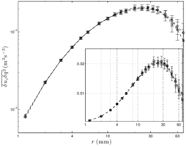
The repeatability of the measurement of was also assessed in a precursory experiment by repeating the same measurement twice (data acquired at the lee of RG60 for the centroid at mm). Comparing the repeatability (a somewhat more stringent test) with the estimated uncertainty (figure 2a), we notice that the confidence intervals are excessively large. This could indicate that the number of independent samples, , based on the integral-time scale, is underestimated. Indeed, splitting the data into integral-time scale sized blocks and extracting a single sample of , leads to estimates of with significantly more scatter, indicating that uncorrelated samples were lost. Instead of using the standard integral time-scale, we can define alternative de-correlation time-scales by taking the autocorrelation of at two times with varying lags and then integrating the resulting correlation functions. This methodology provides a tailored integral time-scale representative of the de-correlation length associated with at each . Assuming that twice this tailored integral time-scale is the characteristic lag between independent samples of we get new estimates of , and consequently new confidence intervals, which are shown in figure 2b. Note that, experiments performed with Particle Imaging Velocimetry obtain reasonable estimates of (see e.g. Lamriben et al., 2011; Danaila et al., 2012) even though the number of independent samples is .
The error bars of the spherically averaged divergence of (figures 7-12) include the confidence intervals plus the error due to the uncertainty of the vertical separation between the X-probe m (see §2.1). The two uncertainties are stacked with a standard propagation of error formula applied to the central differences scheme.
3 Description of the experimental results
The data are acquired with , the midpoint between the two X-probes, along the centreline () at five downstream locations between mm and mm ( and ). For two downstream locations of the centroid, mm and mm, additional datasets off-centreline at mm and are acquired so that derivatives of the statistics with respect to can be computed, particularly those needed to estimate , see (2). The choice of 6mm as the distance to evaluate the -derivative is based on the single-point data in the lee of RG115-turbulence used in I to estimate the lateral triple-correlation transport (i.e. ). Based on those data it is found that the spanwise derivative is well approximated by up to spacings of mm. Too small introduce unnecessary uncertainty to the estimates.
Recall that the X-probes are symmetrically traversed in the y-direction with respect to a fixed , thus enabling the measurement of the statistical correlations as a function of , and that the dependence on is recovered using Taylor’s hypothesis. On the other hand, the traverse mechanism does not allow displacements in the z-direction and the measurements are restricted to the vertical xy-plane at and thus and .
The downstream range of the measurements corresponds to for RG60 and for RG115, a stark difference in the streamwise range relative to owing to the geometrical differences between the grids (see figure 1). In effect, the measurement range for the RG115 corresponds to a nonclassical energy dissipation region whereas for the RG60 it corresponds to a classical one (see Valente and Vassilicos 2012), thus allowing their direct comparison. Recall that the ranges, as well as the straddled Kolmogorov microscales , are comparable for both grids at the chosen measurement locations. Hence the same set up can be used in both experiments without penalising resolution ( versus and versus for RG60- and RG115-generated turbulence, respectively).
Note that the Taylor microscale is calculated as and the Kolmogorov microscale as . The dissipation rate is estimated as (see discussion in §5 of I).
| Location | |||||
|---|---|---|---|---|---|
| Location | |||||
|---|---|---|---|---|---|
3.1 Estimation of the terms in the inhomogeneous Kármán-Howarth-Monin equation
We now describe how the terms appearing in the inhomogeneous Kármán-Howarth-Monin equation (2) are estimated from the present two-component, two-dimensional data using the statistical characteristics of the flow and some additional assumptions.
From the spatially-varying two-component turbulent signals, acquired simultaneously at the transverse separations, the second- and third-order structure functions (, , , , , ) and the mixed structure functions (, , , , ) are computed for all . (Note that are just the transverse separations (mm) and where is the spatial sampling frequency by virtue of Taylor’s hypothesis and are 23 integers chosen to yield approximately the same separation magnitudes as those in the transverse direction.)
The structure functions are then bi-linearly interpolated onto a spherical coordinate system such that is aligned with and with (see figure 3). The grid points in the new coordinate system are located at the interceptions between the 23 circumferences of radius and equally spaced radial lines between the polar angles . After the interpolation, the data is smoothed with a weighted average between each data point at and its neighbours (the total weight of the neighbouring points amounts to ).
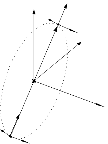
The greatest limitation of the present measurements is lacking the data for the third velocity component, . Lamriben et al. (2011) faced the same limitation in their PIV data which they negotiated by considering the two-component surrogates of the structure functions, which may be sufficient to make qualitative inferences. However, the aim here is to obtain quantitative estimates of the terms in (2). This is achieved by assuming inter-component axisymmetry of the velocity-difference statistics relative to the -axis. In other words, it is assumed that the statistics of the two velocity-difference components perpendicular to ( and , see figure 3) are approximately equal. For the second-order structure function this assumption leads to . Similarly, for the third-order structure functions, and . Note that this assumption is weaker than complete isotropy as it allows for dependence on the orientation . Nevertheless, there is no presently available data to substantiate this assumption and therefore its validity requires further investigation. Even so, it has been verified against all the present data that the added component (i.e. the factor 2 in the equalities two sentences above) does not change the qualitative behaviour of the structure functions, only their magnitude.
Using the processed data, each of the terms in (2), except the pressure transport, is estimated at the measurement plane as follows. Note that the numerical derivatives, both first and second order are computed using a three-point, non-equally spaced central differences scheme Singh and Bhadauria (2009). For equally spaced derivatives this algorithm returns the usual standard central differences scheme.
-
•
since grid-generated turbulence is stationary in the Eulerian frame.
-
•
since the mean flow is approximately parallel, and consequently, the advection in the y- and z-directions is negligible. The streamwise derivatives are actually computed as using the three-point central differences scheme referenced above. Consequently, we use three datasets at different to compute the advection at each for all (recall that there are a total of five datasets with , , , and mm, respectively). Even though the various are coarsely spaced, it has been verified against the present data that the decay of for every can be reasonably approximated with a power-law whose virtual origin coincides with the location of the grid (just as a check of the formula used to compute streamwise derivatives). Also, the longitudinal gradients of the mean velocity are small and therefore we make use of to calculate .
-
•
, i.e. the divergence is computed in the spherical coordinate system and the azimuthal component is assumed to be negligible owing to the axisymmetry of the turbulence statistics with respect to the centreline (see discussion at the end of this subsection). Future work will be required to assess this assumption.
-
•
see Appendix A.
-
•
since and due to the expected symmetry of the mean flow relative to the plane which is parallel to the tunnel’s vertical walls, includes the centreline and cuts the tunnel longitudinally in half. Also note that the symmetry of the mean flow relative to the centreline (leading to , ) has been used to simplify as and as . The transverse gradient is taken from a -order polynomial fit to the mean velocity data at each and the longitudinal gradient is computed as described in the previous item.
-
•
. The transverse derivative ( owing to the symmetry of the turbulence statistics to rotations because of the grid’s geometry) is only computed where the additional off-centreline measurements are acquired. The transverse derivative is simply taken as the difference between centreline and off-centreline data divided by their distance. The derivative with respect to is computed using the various datasets with different . However, this can only be considered as a rough approximation since the various are coarsely spaced. Nevertheless, the longitudinal turbulent transport is typically a small fraction of the lateral transport as was checked against the present two-point data as well as against the single-point transport data presented in §3 of I. The pressure transport, , data cannot be directly estimated with the present apparatus. However, there is no a priori reason to consider it negligible and therefore it is retained in (2) as an unknown. Nevertheless, the contribution from can be inferred indirectly from the deviations of the measured terms’ balance via (2).
-
•
, i.e. only the radial component of the Laplacian is computed. Note that the integrals of the polar, , and azimuthal, , components of the Laplacian over a spherical shell are identically zero, and therefore these terms represent the viscous diffusion across the different orientations . Only spherical shell averages (effectively circumferential averages) are discussed below and therefore the polar and azimuthal components are not computed.
-
•
, see Appendix A.
-
•
, i.e. the centreline energy dissipation estimate is used as a surrogate for the average of the actual dissipation at and (see §5 in I where the different dissipation estimates are discussed). Note that with the present data it is only possible to estimate the dissipation rate along the centerline. Nevertheless, the spanwise profiles of the (less suitable) surrogate indicate that the departures from the centreline value are within , see figure 4d in I.
Of particular importance to the subsequent discussions are the circumferential averages of the terms in (2) in order to remove the dependence on orientation () of the turbulence statistics. The circumferential averages are expected to be good approximations to the averages over spherical shells considering the statistical axisymmetry of the turbulence with respect to the centreline. (Recall that for most of the present data , and therefore , lies along the centreline. However, for the two datasets acquired off-centreline at mm one may expect the validity of this assumption to be more doubtful.) The circumferential averages are obtained by integration with respect to the polar angle as , where the integrand is any one of the measured terms in (2) (note that only one quarter of the domain is used due to the reflection symmetry of the structure functions around the and axes, the former due to stationarity and the latter by construction). The wind tunnel measurements of Nagata et al. (2013) for the decay region in the lee of FSGs and the numerical data of Laizet and Vassilicos (2011) for both FSGs and a RG gives substantial support to this assumption and therefore the circumferential averages are interpreted as spherical shell averages throughout this paper. The spherical shell averaged terms are denoted by removing the superscript asterisk.
3.2 Anisotropy of energy transfer
The anisotropy of the structure functions and is qualitatively investigated from their dependence on . (For notational simplicity and due to the assumed axisymmetry, is not explicitly used as an argument henceforth.) Note that in the present context anisotropy refers to the dependence of the terms in (2) on the orientation (see also Lamriben et al., 2011; Danaila et al., 2012) and not to the kinematic relation between the components of the structure functions parallel and perpendicular to (e.g. versus and versus ), except when clearly indicated. The latter anisotropy considerations are complementary to the first but pertain, for example, to the distribution of kinetic energy between the three orthogonal components and the inter-component energy transfer via pressure fluctuations (see e.g. Sjögren 1997, Sjögren and Johansson, 1998, and references therein).
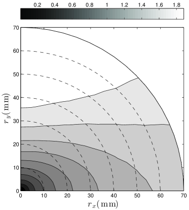
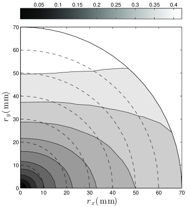
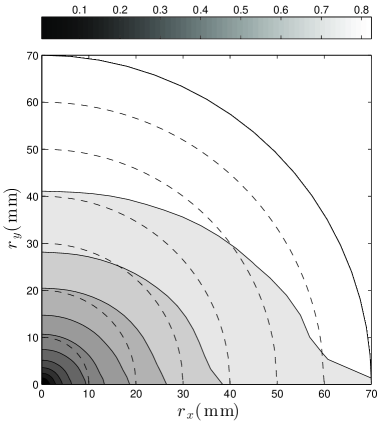
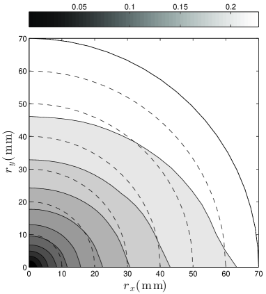
The second-order structure functions are presented in figures 4a-d for the furthermost upstream and downstream measurement locations and for turbulence generated by both RG115 and RG60. Comparing the upstream data (figures 4a,c) with the downstream data (figures 4b,d) for both grids there seems to be a tendency for the contours to become increasingly circular as the turbulence decays, i.e. for the energy distribution to become increasingly isotropic. Furthermore, comparing the RG115 with the RG60 data (figures 4a,b and 4c,d, respectively) it can be seen that the RG115 data, which are acquired closer to the grid in terms of multiples, is less isotropic. Both these observations corroborate a tendency for the kinetic energy to become uniformly distributed over spherical shells for larger . Nevertheless, for all cases the small scales seem to remain anisotropic by velocity derivative measures (see §5 and tables 4 and 5 of I).
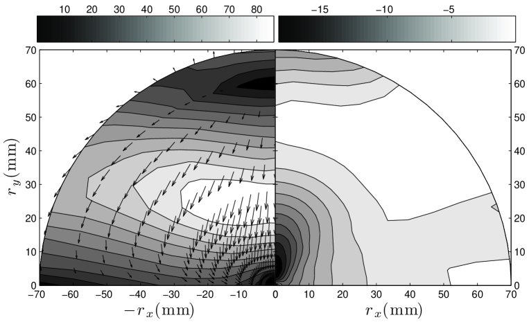
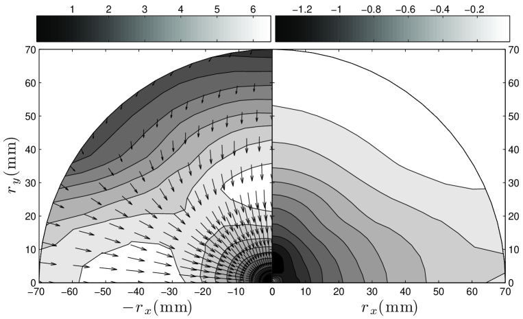
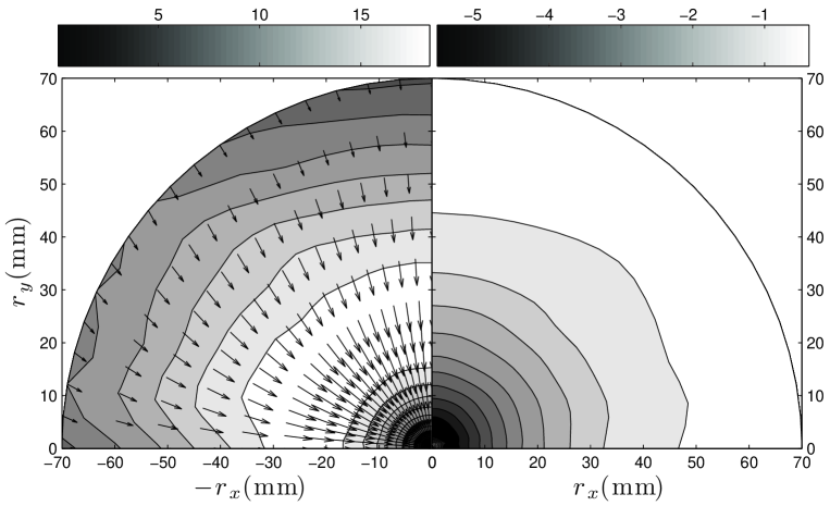
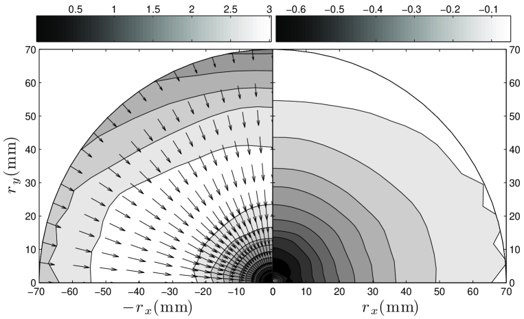
Turning to the third-order structure function vectors , a similar tendency to isotropy is observed (figures 5a,c and 6a,c). The third-order structure function vectors, which for the RG115 data at are nearly aligned with the tangential direction (figure 5a), progressively align with the radial direction and for the RG60 data at (figure 6c) they are indeed nearly so. Note that the divergence of (i.e. ) has a radial and a polar contributions (the azimuthal contribution is taken to be zero due to the assumed axisymmetry). As discussed in §1.2, the radial contribution (which we plot in figures 5b,d and 6b,d) relates to the interscale energy transfer, whereas the polar contribution accounts for the redistribution of energy within a spherical shell. The above mentioned tendency to isotropy as the flow decays is very likely linked to the redistribution of energy via .
4 The role of turbulence production and transport
The effect of transport and production in the single-point kinetic energy balance was investigated in I where it was found that, for the assessed region of the RG115-generated turbulence, both contributions are non-negligible by comparison with the energy dissipation. This region of the RG115-generated turbulence was also compared with an equivalent region of turbulence generated by FSGs and considerable differences were found in the downstream evolution (and transverse profiles) of transport and production relative to the dissipation. Nevertheless, the two different turbulent flows were found to have the same non-classical dissipation behaviour and, consequently, the differences in the production and transport reinforced the view that this non-classical behaviour is present irrespective of the details of the inhomogeneity of the turbulent flow. Indeed, the turbulent transport and production are expected to be large-scale phenomena that play no direct role in the scale-by-scale energy transfer mechanisms, even at these Reynolds numbers (). Here, we present data which allow a precise quantification of the effect of production and transport on the scale-by-scale energy budget (2).
One may average (2) over spherical shells to eliminate the dependence of each term on the orientation yielding the average contribution of each scale to the balance. Retaining all terms except for the linear transfer of energy caused by mean velocity gradients and the scale-by-scale transport by viscous diffusion which were shown to be negligible (see Appendix A), the spherical averaged scale-by-scale energy balance reads,
| (4) |
where the represents the measured component of turbulent transport and represents the unknown contribution from the pressure transport.
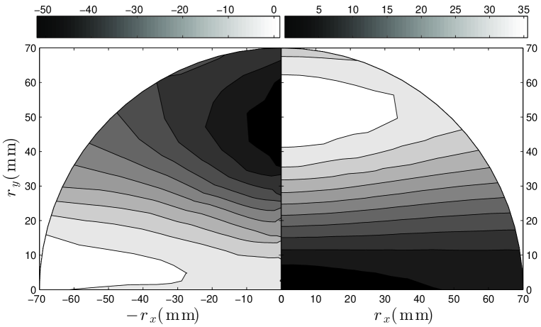
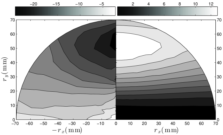
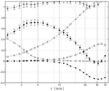
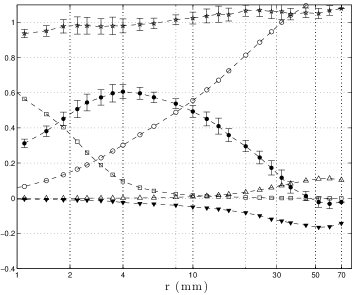
Turning to the data, the iso-contour maps of the transport and production terms normalised by the dissipation, , indicate that most of the transport and production occur at mm and (figures 7a,c and 7b,d). At smaller values of both and are less than about of . Note that the production for large is much smaller for than for because tends to zero at the centreline and the remaining production term, , is small by comparison. Similarly, the transport for large and is also smaller because the lateral transport overwhelms the longitudinal transport.
The spherical averaged contribution of these terms to the balance (4) are plotted together with the spherical shell averaged advection, energy transfer and viscous diffusion in figures 8a,b. Note that the dissipation estimates are compensated for the resolution of the sensor, see §2.2.1 in I. The finite resolution of the sensor also biases since . A rough compensation for this bias is applied by multiplying with the ratio between the corrected and the measured .)
The radial distributions of the advection, energy transfer and viscous diffusion are similar to those found in the literature for data at comparable Reynolds numbers (see e.g. Antonia and Burattini, 2006). From the data it is clear that our turbulent transport and production terms are significant for scales of the order of the integral-length scale but become negligible at scales smaller than and therefore cannot tamper with the scale-by-scale energy transfer around its maximum ( for the present data). This provides quantitative evidence that the influence of the turbulence production and transport on the energy transfer mechanisms is negligible.
Note that in figures 8a,b the balance of the measured terms is also presented. By virtue of (4), the scale-by-scale advection, energy transfer, production, transport and viscous diffusion should balance the dissipation plus the unknown contribution from scale-by-scale pressure transport, . Even though is not accounted for, it can be seen that there is a reasonable balance between the measured terms, at least within the expected uncertainty of the data. Note that the error bars added to the balance (, see figures 8a,b) underestimate the overall uncertainty of the data since they do not take into account uncertainties associated with the measurements of the advection, transport and production terms and possible departures from the assumptions used to compute the terms in (2), see §3.1.
5 Advection, energy transfer and dissipation scalings
We now investigate how the stark differences in the way the energy dissipation scales in the two decay regions identified in Valente and Vassilicos (2012) downstream of a turbulence-generating grid relate to the advection, energy transfer and viscous diffusion during decay (the remaining terms in (4) are negligible at small enough values of as shown in figure 8).
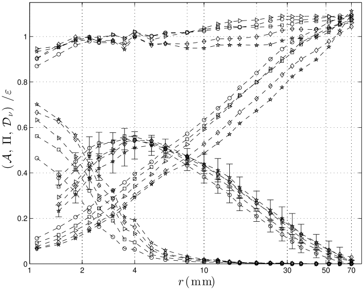
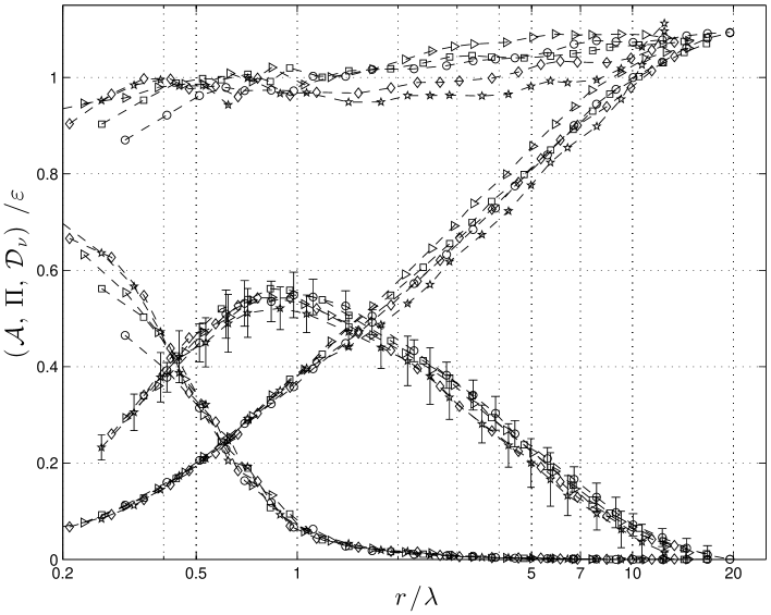
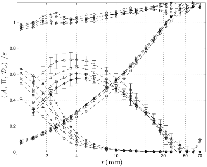
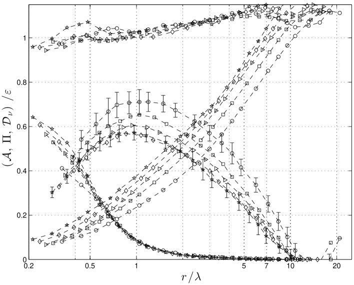
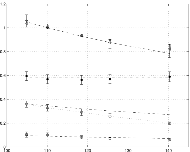
Starting with the RG60 data, the evolution in the further downstream decay region between and of the scale-by-scale viscous diffusion, energy transport and advection normalised by the dissipation are shown in figure 9a. As the turbulence decays these terms seem to move to the right reflecting the increase in the turbulent scales. Normalising the abscissae by seems to account for much of the spread (figure 9b). The scaling of the abscissae is, however, secondary to the main discussion here which pertains to the relative magnitude of the advection, the energy transfer, the viscous diffusion and the dissipation. Note that the viscous diffusion is very small compared to the dissipation at scales for both our RG60 data (see figure 9b) and our RG115 data (figure 10b), in agreement with a mathematical proof of this fact which we give in Appendix B. Of particular importance in figure 9b is the observation that the maximum absolute value of the energy transfer is roughly a constant fraction of the dissipation throughout the downstream extent of the data corresponding to a range of local Reynolds numbers between 100 and 80 ( with the peak located at , see figure 9b).
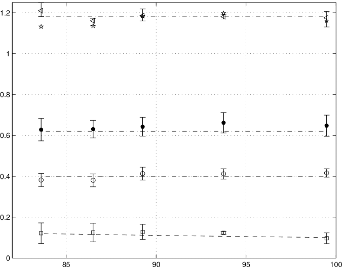
In fact, taking the numerical values of and the numerical values of the advection at the separation where and normalising the data with it is clear from figure 12a that (where , and is the usual longitudinal integral length-scale - for further details refer to I). The viscous diffusion term, is smaller than any of the other terms at this moderate ( of the dissipation) and it is difficult to discern whether is constant or decreases with increasing as one might expect.
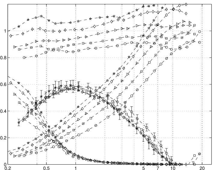
Turning to the RG115 data presented in figure 10a two outstanding differences in the downstream evolution of these quantities can be registered: (i) the peak value of the energy transfer does not scale with the dissipation and (ii) the curves representing the advection term are moving from right to left, in the opposite direction than was the case for the RG60 data (figure 9a). Normalising the abscissae with takes into account most of the spread in the viscous diffusion term but now augments the spread of the advection term (see figure 10b and compare with figure 9b). (Note that for the RG115 data in this region, as shown in Valente and Vassilicos (2012), hence the normalisation of the abscissae with would yield an identical horizontal collapse as that presented in figure 10b). Concerning the scaling of the ordinates, it should be noted that, if instead of one chooses to normalise the ordinates by (figure 11) the vertical spread of the energy transfer data is much reduced, but the spread of the advection is further augmented (as is the spread of the viscous diffusion term, since in the limit this term is equal to the dissipation and, as shown in Valente and Vassilicos (2012), does not scale with in this region).
The procedure of normalising , , and with is repeated and the data are plotted in figure 12b against . Even though the dissipation follows in this region it is clear that the behaviour of is strikingly different. In fact, is approximately constant and with the same numerical value () as the one that we find for the RG60 data in the further downstream region (in multiples of ) where is approximately constant. Note also that the normalised advection term grows faster than with decreasing and therefore adapts to cover most of the growing difference between the constant and the increasing as the flow decays and decreases. The viscous diffusion term is also small for the present data, similar to what is found for the RG60 data.
5.1 Discussion
The present work is concerned with the validity of the energy transfer/dissipation balance over a range of length-scales , i.e.
| (5) |
where instead of using (local) isotropy, is averaged over spherical shells Nie and Tanveer (1999). Note that we have approximated our flow as being locally homogeneous to remove the dependence of the right-hand-side on the separation . We do so based on our RG115 data where is located at mm, cf. figure 10a, corresponding to ; for such close locations no appreciable changes in the dissipation rate can be observed, see figure 4d in I. Finally, note also that in physical space is equal to its wavenumber space counterpart, see appendix C.
It is clear from the outset that the Reynolds numbers of the present data are insufficiently high to allow verification of (5) over a range of length-scales . What the present data do allow us to report for the first time, however, is that (see McComb et al., 2010) both in far downstream equilibrium turbulence where and in non-equilibrium turbulence where and is higher (see figure 12a,b). In this non-equilibrium region our data also demonstrate the growing importance of the small-scale advection with increasing streamwise distance from the grid. This increasing importance is directly linked to the growing imbalance between and (see figure 12b and recall that decreases with increasing streamwise distance in the decay region downstream of the turbulence-generating grid). Note also that the increasing imbalance varies too steeply with compared to the FRN effects discussed by Qian (1999); Moisy et al. (1999); Lundgren (2002, 2003); Gagne et al. (2004); Antonia and Burattini (2006); Tchoufag et al. (2012). In fact, for the Reynolds number range straddled in the present experiments the expected effect of the FRN should be constant throughout the decay as is the case for the equilibrium data in the lee of RG60.
Even though the constancy of is usually expected as a high Reynolds number asymptotic, the equilibrium constancy appears at distances much further downstream in our experiments where the local Reynolds number has in fact further decayed (though, clearly, not enough for not to be constant as a result of the local Reynolds number being too low). The constancy of in this far downstream equilibrium region appears in our RG60 experiments with a rate of change of the local Reynolds number which is enough for to vary in proportion to in the non-equilibrium region (see and compare figures 12a and 12b). Note the high value of the constant in the RG60 equilibrium decay region experiment (figure 12a), high by comparison to values of this constant recorded for forced statistically stationary turbulence and in agreement with time-lag non-equilibrium arguments Bos et al. (2007). What we call the far downstream equilibrium decay region may in fact be a time-lag non-equilibrium region in the terms of Bos et al. (2007). Note that this is a region where there is a ”balance” between the scalings of and (i.e. they both scale as ) whereas such a scaling balance is absent in what we term the non-equilibrium decay region.
6 Conclusion
An experimental investigation of the downstream evolution of the scale-by-scale energy transfer budget for both equilibrium () and non-equilibrium () regular grid-generated decaying turbulence is presented.
We have shown that the turbulent production and transport are large-scale effects which are negligible at length-scales smaller than even though our Reynolds numbers are moderate ( is an integral length-scale taken, here, to be the longitudinal integral length-scale ). Hence, production and transport do not influence the maximum energy transfer to smaller-scales.
The maximum energy transfer rate scales as both in the turbulence decay region which we term non-equilibrium region and in the further downstream turbulence decay region which we term equilibrium region. The non-equilibrium region takes its name from the fact that does not scale as in that region, thus indicating a severe scaling imbalance. In what we term the equilibrium region, and scale in the same way. The imbalance between and in the non-equilibrium region drives the small-scale advection which is non-negligible and increases in proportion to the maximum energy transfer as the turbulence decays. Further downstream where the turbulence decay enters its equilibrium region, the small-scale advection remains about constant in proportion to the maximum energy transfer, presumably until the dissipation loses its high Reynolds number scaling because the local Reynolds number has decayed too much. However, we were not able to access such a very far downstream region in our experiments.
Finally, it should be stressed that the best defined power-law energy spectra with exponents closest to in the grid-generated decaying turbulence have been recorded in the non-equilibrium region Valente and Vassilicos (2012) where, irrespective of the fact that is the Kolmogorov exponent, the lack of balance even in scaling terms between interscale transfer and dissipation indicates a clear non-Richardson-Kolmogorov cascade (see Mazellier and Vassilicos, 2010
and Valente and Vassilicos, 2011).
It is important to know that non-equilibrium cascades such as the ones in the lee of various
grid-generated turbulent flows can follow well-defined scaling laws such as the one for dissipation studied in detail in I and the one for interscale energy transfer established here.
We are grateful to Prof. Arne Johansson (KTH) for the discussion concerning the experimental apparatus. P.C.V would like to thank Anthony R. Oxlade for the help in the digital imaging system setup and Ian Pardew and Roland Hutchins (aero workshop) for the manufacture of the apparatus. P.C.V. acknowledges the financial support from Fundação para a Ciência e a Tecnologia (grant SFRH/BD/61223/2009, cofinanced by POPH/FSE).
Appendix A Estimates of and
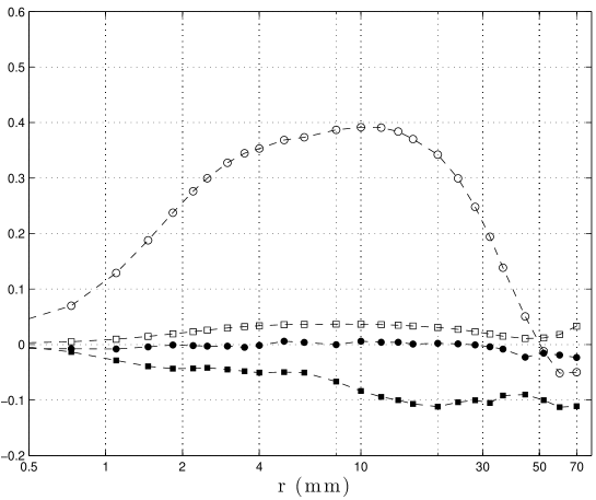
The energy transfer due to mean velocity gradients, , and the transport via viscous diffusion, , are shown to be negligible compared to the other terms in (2). These terms are computed from the acquired data as described in §3.1. As shown in figure 13 the term averaged over spherical shells represents less than of the dissipation at and further downstream, , it decreases to less than . The transport via viscous diffusion averaged over spherical shells, is also negligible and represents less than for both downstream locations, and (see figure 13).
Appendix B A kinematic upper bound for the scale-by-scale viscous diffusion
Under very plausible assumptions on the functional form of
(the second-order structure function averaged over all directions where is the solid angle) we show that the spherical averaged viscous diffusion term appearing in (2) has an upper bound of the form
| (6) |
where is the sum of twice the turbulent kinetic energy at the two locations, and .
This inequality is useful in determining upper ranges of where is negligible by comparison to some other term in (2). Considering, for example, the dissipation term in (2), this inequality can be used to show that if then . In other words, the spherical averaged viscous term is neglible compared to in the upper range of scales where . Clearly is close to a fraction of the Taylor microscale , in fact close to , where turbulent kinetic energy gradients and turbulent dissipation gradients are small and this is indeed the case in the flow regions where the results reported in §5 are observed. One of these results is that is small compared to for (see figures 10b and 11b), a result which can therefore be considered to be a simple kinematic consequence of the inequality established in this Appendix. This conclusion and (6) in general are generalisations in physical space of similar results previously obtained in Fourier space for homogeneous turbulence by a very different method Laizet et al. (2013).
We now proceed by proving the inequalities (6).
We start by writing the Laplacian of in spherical coordinates,
and noting that
Taylor expanding about implies that for small enough values of . At large enough values of , ; more accurately,
We assume (i) that is a monotonically increasing function in with continuous first- and second-order derivatives with respect to ; (ii) that it has only one inflection point at , i.e. only at ; and (iii) that is concave in the range . The monotonicity assumption directly implies that which deals with the second inequality in (6).
The existence of an inflection point is consistent with the commonly observed functional form of where for small r followed by a smooth transition to a power-law of the type with ( for Kolmogorov’s inertial range). The inflection point resides at a value of between these two power laws. The absence of another inflection point agrees with the monotonically increasing passage from the power law to a constant (independent of ).
The assumption that is concave in the range and then monotonically decreasing at is enough to establish that
| (7) |
This can be seen as a geometrical inequality relating the area of the triangle of base and height with the area underneath for . By a similar geometric reasoning for ,
| (8) |
which combined with (7) leads to
| (9) |
Appendix C Equality of in physical and wavenumber space
We note that the maximum nonlinear energy transfer in physical space, , is equal to its wavenumber space counterpart, (, where is the spherical averaged non-linear spectral transfer term, see e.g. Frisch 1995). This can be seen from (6.17) of Frisch (1995), noting that and that (using the book’s notation and defining and ). For a inhomogeneous turbulent flow, care must be taken in guaranteeing existence of the Fourier transform Deissler (1961, 1981).
Contrastingly, it is not straightforward to establish a simple relationship between or and a wavenumber space counterpart, see discussion in §IV of Tchoufag et al. (2012).
References
- Antonia and Burattini (2006) R. A. Antonia and P. Burattini. Approach to the 4/5 law in homogeneous isotropic turbulence. J. Fluid Mech., 550:175–184, 2006.
- Benedict and Gould (1996) L. H. Benedict and R. D. Gould. Towards better uncertainty estimates for turbulent statistics. Exp. Fluids, 22:129–136, 1996.
- Biskamp (2003) D. Biskamp. Magnetohydrodynamic Turbulence. Cambridge University Press, 2003.
- Borue and Orszag (1998) V Borue and S. A. Orszag. Local energy flux and subgrid-scale statistics in three-dimensional turbulence. J. Fluid Mech., 366(1 – 31), 1998.
- Bos et al. (2007) W. J. T. Bos, L. Shao, and J.-P. Bertoglio. Spectral imbalance and the normalized dissipation rate of turbulence. Phys. Fluids, 19(045101), 2007.
- Danaila et al. (2012) L. Danaila, J. F. Krawczynski, F Thiesset, and B. Renou. Yaglom-like equation in axisymmetric anisotropic turbulence. Physica D, 241(3):216–223, 2012.
- de Gennes (1990) P. G. de Gennes. Introduction to polymer dynamics. Cambridge University Press, 1990.
- Deissler (1961) R. G. Deissler. Effects of inhomogeneity and of shear flow in weak turbulent fields. Phys. Fluids, 4(1187), 1961.
- Deissler (1981) R. G. Deissler. Spectral energy transfer for inhomogeneous turbulence. Phys. Fluids, 24(1911), 1981.
- Discetti et al. (2013) S. Discetti, I. B. Ziskin, T. Astarita, R. J. Adrian, and K. P. Prestridge. PIV measurements of anisotropy and inhomogeneity in decaying fractal generated turbulence. Fluid Dyn. Res., Accepted for publication, 2013.
- Frisch (1995) U. Frisch. Turbulence: The Legacy of AN Kolmogorov. Cambridge University Press, Cambridge, 1995.
- Gagne et al. (2004) Y. Gagne, B. Castaing, C. Baudet, and Y. Malecot. Reynolds dependence of third-order structure functions. Phys. Fluids, 16(2):482, 2004.
- George (2013) W. K. George. Reconsidering the ‘Local Equilibrium’ hypothesis for small scale turbulence. Proceedings Marseille (to appear), 2013.
- Gomes-Fernandes et al. (2012) R. Gomes-Fernandes, B. Ganapathisubramani, and J. C. Vassilicos. Particle image velocimetry study of fractal-generated turbulence. J. Fluid Mech., 711:306–336, 2012.
- Kármán and Howarth (1938) T. Kármán and L. Howarth. On the statistical theory of isotropic turbulence. Proc. Roy. Soc. A, 164(917):192–215, 1938.
- Kendall and Stuart (1958) M. G. Kendall and A. Stuart. The advanced theory of statistics, volume 1. Charles Griffin & Co Limited, London, 1958.
- Kolmogorov (1941a) A. N. Kolmogorov. The local structure of turbulence in incompressible viscous fluid for very large reynolds numbers. Dokl. Akad. Nauk. SSSR, 30(4), 1941a. (Reprinted in 1991, Proc. R. Soc. Lond., Vol. 434, pp. 9-13).
- Kolmogorov (1941c) A. N. Kolmogorov. Dissipation of energy in the locally isotropic turbulence. Dokl. Akad. Nauk. SSSR, 32(1), 1941c. (Reprinted in 1991, paper 47 in Selected Works of A.N. Kolmogorov, Vol. I: Mathematics and Mechanics).
- Kraichnan (1974) R. Kraichnan. On Kolmogorov’s inertial-range theories. J. Fluid Mech., 62(2):305 – 330, 1974.
- Laizet and Vassilicos (2011) S. Laizet and J. C. Vassilicos. DNS of fractal-generated turbulence. Flow Turb. Combust., pages 87:673–705, 2011.
- Laizet et al. (2013) S. Laizet, J. C. Vassilicos, and C. Cambon. Interscale energy transfer in decaying turbulence and vorticity-strain dynamics in grid-generated turbulence. Fluid Dyn. Res. (to appear October 2013), 2013.
- Lamriben et al. (2011) C. Lamriben, P.-P. Cortet, and F. Moisy. Direct measurements of anisotropic energy transfers in a rotating turbulence experiment. Phys. Rev. Lett., 107(024503), 2011.
- Lumley (1992) J. L. Lumley. Some comments on turbulence. Phys. Fluids A, 4(2):203–211, 1992.
- Lundgren (2002) T. S. Lundgren. Kolmogorov two-thirds law by matched asymptotic expansion. Phys. Fluids, 14(2), 2002.
- Lundgren (2003) T. S. Lundgren. Kolmogorov turbulence by matched asymptotic expansion. Phys. Fluids, 15(4), 2003.
- Marati et al. (2004) N. Marati, C. M. Casciola, and R. Piva. Energy cascade and spatial fluxes in wall turbulence. J. Fluid Mech., 521:191–215, 2004.
- Mazellier and Vassilicos (2010) N. Mazellier and J. C. Vassilicos. Turbulence without Richardson-Kolmogorov cascade. Phys. Fluids, 22:075101, 2010.
- McComb et al. (2010) W. D. McComb, A. Berera, M. Salewski, and S. Yoffe. Taylor’s (1935) dissipation surrogate reinterpreted. Phys. Fluids, 22(061704), 2010.
- Moisy et al. (1999) F. Moisy, P. Tabeling, and H. Wilaime. Kolmogorov equation in a fully developed turbulence experiment. Phys. Rev. E, 82(20):3994, 1999.
- Monin and Yaglom (1975) A.S. Monin and A.M. Yaglom. Statistical Fluid Mechanics, volume Vol. 2. MIT Press, 1975.
- Nagata et al. (2013) K. Nagata, Y. Sakai, T. Inaba, H. Suzuki, O. Terashima, and H. Suzuki. Turbulence structure and turbulence kinetic energy transport in multiscale/fractal-generated turbulence. Phys. Fluids, 25(065102), 2013.
- Nie and Tanveer (1999) Q. Nie and S. Tanveer. A note on third-order structure functions in turbulence. Proc. R. Soc. Lond. A, 455:1615–1635, 1999.
- Qian (1999) J. Qian. Slow decay of the finite reynolds number effect of turbulence. Phys. Rev. E, 60(3), 1999.
- Rubinstein and Bos (2009) R. Rubinstein and W. J. T. Bos. On the unsteady behavior of turbulence models. Phys. Fluids, 21(041701), 2009.
- Schiestel (1987) R. Schiestel. Multiple-time-scale modeling of turbulent flows in one point closures. Phys. Fluids, 30(722), 1987.
- Singh and Bhadauria (2009) A. K. Singh and B. S. Bhadauria. Finite difference formulae for unequal sub-intervals using Lagrange’s interpolation formula. Int. J. Math. Anal., 3(17), 2009.
- Sjögren (1997) T. Sjögren. Development and Validation of Turbulence Models Through Experiment and Computation. PhD thesis, Royal Institute of Technology (K.T.H.), 1997.
- Sjögren and Johansson (1998) T. Sjögren and A. V. Johansson. Measurement and modelling of homogeneous axisymmetric turbulence. J. Fluid Mech., 374:59–90, 1998.
- Tchoufag et al. (2012) J. Tchoufag, P. Sagaut, and C. Cambon. Spectral approach to finite Reynolds number effects on Kolmogorov’s 4/5 law in isotropic turbulence. Phys. Fluids, 24(015107), 2012.
- Valente and Vassilicos (2011) P. C. Valente and J. C. Vassilicos. The decay of turbulence generated by a class of multi-scale grids. J. Fluid Mech., 687:300–340, 2011.
- Valente and Vassilicos (2012) P. C. Valente and J. C. Vassilicos. Universal dissipation scaling for nonequilibrium turbulence. Phys. Rev. Lett., 108(214503), 2012.
- Valente and Vassilicos (2014) P. C. Valente and J. C. Vassilicos. The nonequilibrium region of grid-generated turbulence. J. Fluid Mech. (in press), 2014.
- Wan et al. (2010) M. Wan, Z. Xiao, C. Meneveau, G. L. Eyink, and S. Chen. Dissipation-energy flux correlations as evidence for the lagrangian energy cascade in turbulence. Phys. Fluids, 22(061702), 2010.
- Yoshizawa (1994) A. Yoshizawa. Nonequilibrium effect of the turbulent-energy-production process on the inertial-range spectrum. Phys. Rev. E, 49(5), 1994.