Kernel Adaptive Metropolis-Hastings
Abstract
A Kernel Adaptive Metropolis-Hastings algorithm is introduced, for the purpose of sampling from a target distribution with strongly nonlinear support. The algorithm embeds the trajectory of the Markov chain into a reproducing kernel Hilbert space (RKHS), such that the feature space covariance of the samples informs the choice of proposal. The procedure is computationally efficient and straightforward to implement, since the RKHS moves can be integrated out analytically: our proposal distribution in the original space is a normal distribution whose mean and covariance depend on where the current sample lies in the support of the target distribution, and adapts to its local covariance structure. Furthermore, the procedure requires neither gradients nor any other higher order information about the target, making it particularly attractive for contexts such as Pseudo-Marginal MCMC. Kernel Adaptive Metropolis-Hastings outperforms competing fixed and adaptive samplers on multivariate, highly nonlinear target distributions, arising in both real-world and synthetic examples.
1 Introduction
The choice of the proposal distribution is known to be crucial for the design of Metropolis-Hastings algorithms, and methods for adapting the proposal distribution to increase the sampler’s efficiency based on the history of the Markov chain have been widely studied. These methods often aim to learn the covariance structure of the target distribution, and adapt the proposal accordingly. Adaptive MCMC samplers were first studied by Haario et al. (1999, 2001), where the authors propose to update the proposal distribution along the sampling process. Based on the chain history, they estimate the covariance of the target distribution and construct a Gaussian proposal centered at the current chain state, with a particular choice of the scaling factor from Gelman et al. (1996). More sophisticated schemes are presented by Andrieu & Thoms (2008), e.g., adaptive scaling, component-wise scaling, and principal component updates.
While these strategies are beneficial for distributions that show high anisotropy (e.g., by ensuring the proposal uses the right scaling in all principal directions), they may still suffer from low acceptance probability and slow mixing when the target distributions are strongly nonlinear, and the directions of large variance depend on the current location of the sampler in the support. In the present work, we develop an adaptive Metropolis-Hastings algorithm in which samples are mapped to a reproducing kernel Hilbert space, and the proposal distribution is chosen according to the covariance in this feature space (Schölkopf et al., 1998; Smola et al., 2001). Unlike earlier adaptive approaches, the resulting proposal distributions are locally adaptive in input space, and oriented towards nearby regions of high density, rather than simply matching the global covariance structure of the distribution. Our approach combines a move in the feature space with a stochastic step towards the nearest input space point, where the feature space move can be analytically integrated out. Thus, the implementation of the procedure is straightforward: the proposal is simply a multivariate Gaussian in the input space, with location-dependent covariance which is informed by the feature space representation of the target. Furthermore, the resulting Metropolis-Hastings sampler only requires the ability to evaluate the unnormalized density of the target (or its unbiased estimate, as in Pseudo-Marginal MCMC of Andrieu & Roberts, 2009), and no gradient evaluation is needed, making it applicable to situations where more sophisticated schemes based on Hamiltonian Monte Carlo (HMC) or Metropolis Adjusted Langevin Algorithms (MALA) (Roberts & Stramer, 2003; Girolami & Calderhead, 2011) cannot be applied.
We begin our presentation in Section 2, with a brief overview of existing adaptive Metropolis approaches; we also review covariance operators in the RKHS. Based on these operators, we describe a sampling strategy for Gaussian measures in the RKHS in Section 3, and introduce a cost function for constructing proposal distributions. In Section 4, we outline our main algorithm, termed Kernel Adaptive Metropolis-Hastings (MCMC Kameleon). We provide experimental comparisons with other fixed and adaptive samplers in Section 5, where we show superior performance in the context of Pseudo-Marginal MCMC for Bayesian classification, and on synthetic target distributions with highly nonlinear shape.
2 Background
Adaptive Metropolis Algorithms.
Let be the domain of interest, and denote the unnormalized target density on by . Additionally, let denote an estimate of the covariance matrix of the target density based on the chain history . The original adaptive Metropolis at the current state of the chain state uses the proposal
| (1) |
where is a fixed scaling factor from Gelman et al. (1996). This choice of scaling factor was shown to be optimal (in terms of efficiency measures) for the usual Metropolis algorithm. While this optimality result does not hold for Adaptive Metropolis, it can nevertheless be used as a heuristic. Alternatively, the scale can also be adapted at each step as in Andrieu & Thoms (2008, Algorithm 4) to obtain the acceptance rate from Gelman et al. (1996), .
RKHS Embeddings and Covariance Operators.
According to the Moore-Aronszajn theorem (Berlinet & Thomas-Agnan, 2004, p. 19), for every symmetric, positive definite function (kernel) , there is an associated reproducing kernel Hilbert space of real-valued functions on with reproducing kernel . The map , is called the canonical feature map of . This feature map or embedding of a single point can be extended to that of a probability measure on : its kernel embedding is an element , given by (Berlinet & Thomas-Agnan, 2004; Fukumizu et al., 2004; Smola et al., 2007). If a measurable kernel is bounded, it is straightforward to show using the Riesz representation theorem that the mean embedding exists for all probability measures on . For many interesting bounded kernels , including the Gaussian, Laplacian and inverse multi-quadratics, the kernel embedding is injective. Such kernels are said to be characteristic (Sriperumbudur et al., 2010, 2011), since each distribution is uniquely characterized by its embedding (in the same way that every probability distribution has a unique characteristic function). The kernel embedding is the representer of expectations of smooth functions w.r.t. , i.e., , . Given samples , the embedding of the empirical measure is .
Next, the covariance operator for a probability measure is given by (Baker, 1973; Fukumizu et al., 2004), where for the tensor product is defined as . The covariance operator has the property that , .
Our approach is based on the idea that the nonlinear support of a target density may be learned using Kernel Principal Component Analysis (Kernel PCA) (Schölkopf et al., 1998; Smola et al., 2001), this being linear PCA on the empirical covariance operator in the RKHS, , computed on the sample defined above. The empirical covariance operator behaves as expected: applying the tensor product definition gives . By analogy with algorithms which use linear PCA directions to inform M-H proposals (Andrieu & Thoms, 2008, Algorithm 8), nonlinear PCA directions can be encoded in the proposal construction, as described in Appendix C. Alternatively, one can focus on a Gaussian measure on the RKHS determined by the empirical covariance operator rather than extracting its eigendirections, which is the approach we pursue in this contribution. This generalizes the proposal (1), which considers the Gaussian measure induced by the empirical covariance matrix on the original space.
3 Sampling in RKHS
We next describe the proposal distribution at iteration of the MCMC chain. We will assume that a subset of the chain history, denoted , , is available. Our proposal is constructed by first considering the samples in the RKHS associated to the empirical covariance operator, and then performing a gradient descent step on a cost function associated with those samples.
Gaussian Measure of the Covariance Operator.
We will work with the Gaussian measure on the RKHS with mean and covariance , where is the subset of the chain history. While there is no analogue of a Lebesgue measure in an infinite dimensional RKHS, it is instructive (albeit with some abuse of notation) to denote this measure in the “density form” . As is a finite-rank operator, this measure is supported only on a finite-dimensional affine space , where is the subspace spanned by the canonical features of . It can be shown that a sample from this measure has the form where is isotropic. Indeed, to see that has the correct covariance structure, note that:
Due to the equivalence in the RKHS between a Gaussian measure and a Gaussian Process (GP) (Berlinet & Thomas-Agnan, 2004, Ch. 4), we can think of the RKHS samples as trajectories of the GP with mean and covariance function
The covariance function of this GP is therefore the kernel convolved with itself with respect to the empirical measure associated to the samples , and draws from this GP therefore lie in a smaller RKHS; see Saitoh (1997, p. 21) for details.
Obtaining Target Samples through Gradient Descent.
We have seen how to obtain the RKHS sample from the Gaussian measure in the RKHS. This sample does not in general have a corresponding pre-image in the original domain ; i.e., there is no point such that . If there were such a point, then we could use it as a proposal in the original domain. Therefore, we are ideally looking for a point whose canonical feature map is close to in the RKHS norm. We consider the optimization problem
In general, this is a non-convex minimization problem, and may be difficult to solve (Bakir et al., 2003). Rather than solving it for every new vector of coefficients , which would lead to an excessive computational burden for every proposal made, we simply make a single descent step along the gradient of the cost function,
| (2) |
i.e., the proposed new point is
where is a gradient step size parameter and is an additional isotropic ’exploration’ term after the gradient step. It will be useful to split the scaled gradient at into two terms as , where ,
| (3) |
is a matrix, and is the centering matrix.
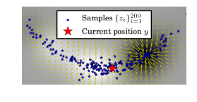
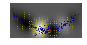
Figure 1 plots and its gradients for several samples of -coefficients, in the case where the underlying -samples are from the two-dimensional nonlinear Banana target distribution of Haario et al. (1999). It can be seen that may have multiple local minima, and that it varies most along the high-density regions of the Banana distribution.
4 MCMC Kameleon Algorithm
MCMC Kameleon
Input: unnormalized target , subsample size , scaling parameters adaptation probabilities , kernel ,
4.1 Proposal Distribution
We now have a recipe to construct a proposal that is able to adapt to the local covariance structure for the current chain state . This proposal depends on a subset of the chain history , and is denoted by . While we will later simplify this proposal by integrating out the moves in the RKHS, it is instructive to think of the proposal generating process as:
-
1.
Sample ( normal of RKHS coefficients).
-
•
This represents an RKHS sample which is the goal of the cost function .
-
•
-
2.
Move along the gradient of :
-
•
This gives a proposal ( normal in the original space).
-
•
Our first step in the derivation of the explicit proposal density is to show that as long as is a differentiable positive definite kernel, the term vanishes.
Proposition 1.
Let be a differentiable positive definite kernel. Then .
Since , the gradient step size always appears together with , so we merge and the scale of the -coefficients into a single scale parameter, and set henceforth. Furthermore, since both and are multivariate Gaussian densities, the proposal density can be computed analytically. We therefore get the following closed form expression for the proposal distribution.
Proposition 2.
.
Proofs of the above Propositions are given in Appendix A.
With the derived proposal distribution, we proceed with the standard Metropolis-Hastings accept/reject scheme, where the proposed sample is accepted with probability
| (4) |
giving rise to the MCMC Kameleon Algorithm. Note that each and could be replaced by their unbiased estimates without impacting the invariant distribution (Andrieu & Roberts, 2009).
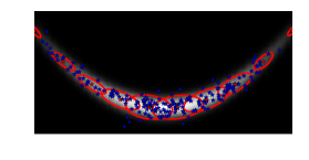
The constructed family of proposals encodes local structure of the target distribution, which is learned based on the subsample . Figure 2 depicts the regions that contain 95% of the mass of the proposal distribution at various states for a fixed subsample , where the Banana target is used (details in Section 5). More examples of proposal contours can be found in Appendix B.
4.2 Properties of the Algorithm
The update schedule and convergence.
MCMC Kameleon requires a subsample at each iteration of the algorithm, and the proposal distribution is updated each time a new subsample is obtained. It is well known that a chain which keeps adapting the proposal distribution need not converge to the correct target (Andrieu & Thoms, 2008). To guarantee convergence, we introduce adaptation probabilities , such that and , and at iteration we update the subsample with probability . As adaptations occur with decreasing probability, Theorem 1 of Roberts & Rosenthal (2007) implies that the resulting algorithm is ergodic and converges to the correct target. Another straightforward way to guarantee convergence is to fix the set after a “burn-in” phase; i.e., to stop adapting Roberts & Rosenthal (2007, Proposition 2). In this case, a “burn-in” phase is used to get a rough sketch of the shape of the distribution: the initial samples need not come from a converged or even valid MCMC chain, and it suffices to have a scheme with good exploratory properties, e.g., Welling & Teh (2011). In MCMC Kameleon, the term allows exploration in the initial iterations of the chain (while the subsample is still not informative about the structure of the target) and provides regularization of the proposal covariance in cases where it might become ill-conditioned. Intuitively, a good approach to setting is to slowly decrease it with each adaptation, such that the learned covariance progressively dominates the proposal.
Symmetry of the proposal.
In Haario et al. (2001), the proposal distribution is asymptotically symmetric due to the vanishing adaptation property. Therefore, the authors compute the standard Metropolis acceptance probability. In our case, the proposal distribution is a Gaussian with mean at the current state of the chain and covariance , where depends both on the current state and a random subsample of the chain history . This proposal distribution is never symmetric (as covariance of the proposal always depends on the current state of the chain), and therefore we use the Metropolis-Hastings acceptance probability to reflect this.
Relationship to MALA and Manifold MALA.
The Metropolis Adjusted Langevin Algorithm (MALA) algorithm uses information about the gradient of the log-target density at the current chain state to construct a proposed point for the Metropolis step. Our approach does not require that the log-target density gradient be available or computable. Kernel gradients in the matrix are easily obtained for commonly used kernels, including the Gaussian kernel (see section 4.3), for which the computational complexity is equal to evaluating the kernel itself. Moreover, while standard MALA simply shifts the mean of the proposal distribution along the gradient and then adds an isotropic exploration term, our proposal is centered at the current state, and it is the covariance structure of the proposal distribution that coerces the proposed points to belong to the high-density regions of the target. It would be straightforward to modify our approach to include a drift term along the gradient of the log-density, should such information be available, but it is unclear whether this would provide additional performance gains. Further work is required to elucidate possible connections between our approach and the use of a preconditioning matrix (Roberts & Stramer, 2003) in the MALA proposal; i.e., where the exploration term is scaled with appropriate metric tensor information, as in Riemannian manifold MALA (Girolami & Calderhead, 2011).
4.3 Examples of Covariance Structure for Standard Kernels
The proposal distributions in MCMC Kameleon are dependant on the choice of the kernel . To gain intuition regarding their covariance structure, we give two examples below.
Linear kernel.
In the case of a linear kernel , we obtain , so the proposal is given by ; thus, the proposal simply uses the scaled empirical covariance just like standard Adaptive Metropolis (Haario et al., 1999), with an additional isotropic exploration component, and depends on only through the mean.
Gaussian kernel.
In the case of a Gaussian kernel , since , we obtain
Consider how this encodes the covariance structure of the target distribution:
| (5) | |||||
As the first two terms dominate, the previous points which are close to the current state (for which is large) have larger weights, and thus they have more influence in determining the covariance of the proposal at .
Matérn kernel.
In the Matérn family of kernels , where is the modified Bessel function of the second kind, we obtain a form of the covariance structure very similar to that of the Gaussain kernel. In this case, , so the only difference (apart from the scalings) to (5) is that the weights are now determined by a “rougher” kernel of the same family.
5 Experiments
In the experiments, we compare the following samplers: (SM) Standard Metropolis with the isotropic proposal and scaling , (AM-FS) Adaptive Metropolis with a learned covariance matrix and fixed scaling , (AM-LS) Adaptive Metropolis with a learned covariance matrix and scaling learned to bring the acceptance rate close to as described in Andrieu & Thoms (2008, Algorithm 4), and (KAMH-LS) MCMC Kameleon with the scaling learned in the same fashion ( was fixed to 0.2), and which also stops adapting the proposal after the burn-in of the chain (in all experiments, we use a random subsample of size , and a Gaussian kernel with bandwidth selected according to the median heuristic). We consider the following nonlinear targets: (1) the posterior distribution of Gaussian Process (GP) classification hyperparameters (Filippone & Girolami, 2014) on the UCI glass dataset, and (2) the synthetic banana-shaped distribution of Haario et al. (1999) and a flower-shaped disribution concentrated on a circle with a periodic perturbation.
5.1 Pseudo-Marginal MCMC for GP Classification
Moderately twisted 8-dimensional target; iterations: 40000, burn-in: 20000

Strongly twisted 8-dimensional target; iterations: 80000, burn-in: 40000

8-dimensional target; iterations: 120000, burn-in: 60000

In the first experiment, we illustrate usefulness of the MCMC Kameleon sampler in the context of Bayesian classification with GPs (Williams & Barber, 1998). Consider the joint distribution of latent variables , labels (with covariate matrix ), and hyperparameters , given by
where , with modeling the covariance between latent variables evaluated at the input covariates: and . We restrict our attention to the binary logistic classifier; i.e., the likelihood is given by where . We pursue a fully Bayesian treatment, and estimate the posterior of the hyperparameters . As observed by Murray & Adams (2012), a Gibbs sampler on , which samples from and in turn, is problematic, as is extremely sharp, drastically limiting the amount that any Markov chain can update . On the other hand, if we directly consider the marginal posterior of the hyperparameters, a much less peaked distribution can be obtained. However, the marginal likelihood is intractable for non-Gaussian likelihoods , so it is not possible to analytically integrate out the latent variables. Recently developed pseudo-marginal MCMC methods (Andrieu & Roberts, 2009) enable exact inference on this problem (Filippone & Girolami, 2014), by replacing with an unbiased estimate
| (6) |
where are importance samples. In Filippone & Girolami (2014), the importance distribution is chosen as the Laplacian or as the Expectation Propagation (EP) approximation of , leading to state-of-the-art results.
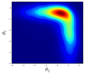
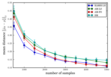
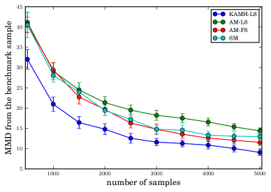
We consider the UCI Glass dataset (Bache & Lichman, 2013), where classification of window against non-window glass is sought. Due to the heterogeneous structure of each of the classes (i.e., non-window glass consists of containers, tableware and headlamps), there is no single consistent set of lengthscales determining the decision boundary, so one expects the posterior of the covariance bandwidths to have a complicated (nonlinear) shape. This is illustrated by the plot of the posterior projections to the dimensions 2 and 7 (out of 9) in Figure 3. Since the ground truth for the hyperparameter posterior is not available, we initially ran 30 Standard Metropolis chains for 500,000 iterations (with a 100,000 burn-in), kept every 1000-th sample in each of the chains, and combined them. The resulting samples were used as a benchmark, to evaluate the performance of shorter single-chain runs of SM, AM-FS, AM-LS and KAMH-LS. Each of these algorithms was run for 100,000 iterations (with a 20,000 burnin) and every 20-th sample was kept. Two metrics were used in evaluating the performance of the four samplers, relative to the large-scale benchmark. First, the distance was computed between the mean estimated from each of the four sampler outputs, and the mean on the benchmark sample (Fig. 4, left), as a function of sample size. Second, the MMD (Borgwardt et al., 2006; Gretton et al., 2007) was computed between each sampler output and the benchmark sample, using the polynomial kernel ; i.e., the comparison was made in terms of all mixed moments of order up to 3 (Fig. 4, right). The figures indicate that KAMH-LS approximates the benchmark sample better than the competing approaches, where the effect is especially pronounced in the high order moments, indicating that KAMH-LS thoroughly explores the distribution support in a relatively small number of samples.
We emphasise that, as for any pseudo-marginal MCMC scheme, neither the likelihood itself, nor any higher-order information about the marginal posterior target , are available. This makes HMC or MALA based approaches such as (Roberts & Stramer, 2003; Girolami & Calderhead, 2011) unsuitable for this problem, so it is very difficult to deal with strongly nonlinear posterior targets. In contrast, as indicated in this example, the MCMC Kameleon scheme is able to effectively sample from such nonlinear targets, and outperforms the vanilla Metropolis methods, which are the only competing choices in the pseudo-marginal context.
In addition, since the bulk of the cost for pseudo-marginal MCMC is in importance sampling in order to obtain the acceptance ratio, the additional cost imposed by KAMH-LS is negligible. Indeed, we observed that there is an increase of only 2-3% in terms of effective computation time in comparison to all other samplers, for the chosen size of the chain history subsample ().
5.2 Synthetic examples
Banana target.
In Haario et al. (1999), the following family of nonlinear target distributions is considered. Let be a multivariate normal in dimensions, with , which undergoes the transformation , where , and for . We will write . It is clear that , and that
Flower target.
The second target distribution we consider is the -dimensional flower target , with
This distribution concentrates around the -circle with a periodic perturbation (with amplitude and frequency ) in the first two dimensions.
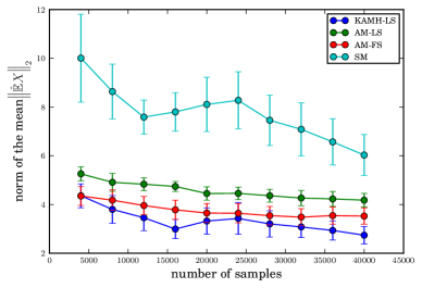
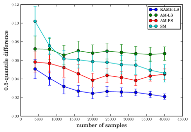
In these examples, exact quantile regions of the targets can be computed analytically, so we can directly assess performance without the need to estimate distribution distances on the basis of samples (i.e., by estimating MMD to the benchmark sample). We compute the following measures of performance (similarly as in Haario et al. (1999); Andrieu & Thoms (2008)) based on the chain after burn-in: average acceptance rate, norm of the empirical mean (the true mean is by construction zero for all targets), and the deviation of the empirical quantiles from the true quantiles. We consider 8-dimensional target distributions: the moderately twisted banana target (Figure 5, top) and the strongly twisted banana target (Figure 5, middle) and flower target (Figure 5, bottom).
The results show that MCMC Kameleon is superior to the competing samplers. Since the covariance of the proposal adapts to the local structure of the target at the current chain state, as illustrated in Figure 2, MCMC Kameleon does not suffer from wrongly scaled proposal distributions. The result is a significantly improved quantile performance in comparison to all competing samplers, as well as a comparable or superior norm of the empirical mean. SM has a significantly larger norm of the empirical mean, due to its purely random walk behavior (e.g., the chain tends to get stuck in one part of the space, and is not able to traverse both tails of the banana target equally well). AM with fixed scale has a low acceptance rate (indicating that the scaling of the proposal is too large), and even though the norm of the empirical mean is much closer to the true value, quantile performance of the chain is poor. Even if the estimated covariance matrix closely resembles the true global covariance matrix of the target, using it to construct proposal distributions at every state of the chain may not be the best choice. For example, AM correctly captures scalings along individual dimensions for the flower target (the norm of its empirical mean is close to its true value of zero) but fails to capture local dependence structure. The flower target, due to its symmetry, has an isotropic covariance in the first two dimensions – even though they are highly dependent. This leads to a mismatch in the scale of the covariance and the scale of the target, which concentrates on a thin band in the joint space. AM-LS has the “correct” acceptance rate, but the quantile performance is even worse, as the scaling now becomes too small to traverse high-density regions of the target.
6 Conclusions
We have constructed a simple, versatile, adaptive, gradient-free MCMC sampler that constructs a family of proposal distributions based on the sample history of the chain. These proposal distributions automatically conform to the local covariance structure of the target distribution at the current chain state. In experiments, the sampler outperforms existing approaches on nonlinear target distributions, both by exploring the entire support of these distributions, and by returning accurate empirical quantiles, indicating faster mixing. Possible extensions include incorporating additional parametric information about the target densities, and exploring the tradeoff between the degree of sub-sampling of the chain history and convergence of the sampler.
Software.
Python implementation of MCMC Kameleon is available at https://github.com/karlnapf/kameleon-mcmc.
Acknowledgments.
D.S., H.S., M.L.G. and A.G. acknowledge support of the Gatsby Charitable Foundation. We thank Mark Girolami for insightful discussions and the anonymous reviewers for useful comments.
References
- Andrieu & Roberts (2009) Andrieu, C. and Roberts, G.O. The pseudo-marginal approach for efficient Monte Carlo computations. Ann. Statist., 37(2):697–725, 2009.
- Andrieu & Thoms (2008) Andrieu, C. and Thoms, J. A tutorial on adaptive MCMC. Statistics and Computing, 18(4):343–373, 2008.
- Bache & Lichman (2013) Bache, K. and Lichman, M. UCI Machine Learning Repository, 2013. URL http://archive.ics.uci.edu/ml.
- Baker (1973) Baker, C. Joint measures and cross-covariance operators. Transactions of the American Mathematical Society, 186:273–289, 1973.
- Bakir et al. (2003) Bakir, G., Weston, J., and Schölkopf, B. Learning to find pre-images. In Advances in Neural Information Processing Systems 16. MIT Press, 2003.
- Berlinet & Thomas-Agnan (2004) Berlinet, A. and Thomas-Agnan, C. Reproducing Kernel Hilbert Spaces in Probability and Statistics. Kluwer, 2004.
- Borgwardt et al. (2006) Borgwardt, K. M., Gretton, A., Rasch, M. J., Kriegel, H.-P., Schölkopf, B., and Smola, A. J. Integrating structured biological data by kernel maximum mean discrepancy. Bioinformatics (ISMB), 22(14):e49–e57, 2006.
- Filippone & Girolami (2014) Filippone, M. and Girolami, M. Pseudo-marginal Bayesian inference for Gaussian Processes. IEEE Transactions on Pattern Analysis and Machine Intelligence, 2014. doi: TPAMI.2014.2316530.
- Fukumizu et al. (2004) Fukumizu, K., Bach, F. R., and Jordan, M. I. Dimensionality reduction for supervised learning with reproducing kernel Hilbert spaces. J. Mach. Learn. Res., 5:73–99, 2004.
- Gelman et al. (1996) Gelman, A., Roberts, G. O., and Gilks, W. R. Efficient Metropolis jumping rules. In Bayesian statistics, 5 (Alicante, 1994), Oxford Sci. Publ., pp. 599–607. 1996.
- Girolami & Calderhead (2011) Girolami, M. and Calderhead, B. Riemann manifold Langevin and Hamiltonian Monte Carlo methods. Journal of the Royal Statistical Society: Series B, 73(2):123–214, 2011.
- Gretton et al. (2007) Gretton, A., Borgwardt, K., Rasch, M., Schölkopf, B., and Smola, A. A kernel method for the two-sample problem. In Advances in Neural Information Processing Systems 19, pp. 513–520, 2007.
- Haario et al. (1999) Haario, H., Saksman, E., and Tamminen, J. Adaptive Proposal Distribution for Random Walk Metropolis Algorithm. Comput. Stat., 14(3):375–395, 1999.
- Haario et al. (2001) Haario, H., Saksman, E., and Tamminen, J. An adaptive Metropolis algorithm. Bernoulli, 7(2):223–242, 2001.
- Murray & Adams (2012) Murray, I. and Adams, R.P. Slice sampling covariance hyperparameters of latent Gaussian models. In Advances in Neural Information Processing Systems 23. 2012.
- Roberts & Rosenthal (2007) Roberts, G.O. and Rosenthal, J.S. Coupling and ergodicity of adaptive Markov chain Monte Carlo algorithms. J. Appl. Probab., 44(2):458–475, 03 2007.
- Roberts & Stramer (2003) Roberts, G.O. and Stramer, O. Langevin diffusions and Metropolis-Hastings algorithms. Methodol. Comput. Appl. Probab., 4:337–358, 2003.
- Saitoh (1997) Saitoh, S. Integral transforms, reproducing kernels, and their applications. Pitman Research Notes in Mathematics 369, Longman Scientific & Techn., 1997.
- Schölkopf et al. (1998) Schölkopf, B., Smola, A. J., and Müller, K.-R. Nonlinear component analysis as a kernel eigenvalue problem. Neural Comput., 10:1299–1319, 1998.
- Smola et al. (2007) Smola, A., Gretton, A., Song, L., and Schölkopf, B. A Hilbert space embedding for distributions. In Proceedings of the Conference on Algorithmic Learning Theory (ALT), pp. 13–31. Springer, 2007.
- Smola et al. (2001) Smola, A. J., Mika, S., Schölkopf, B., and Williamson, R. C. Regularized principal manifolds. J. Mach. Learn. Res., 1:179–209, 2001.
- Sriperumbudur et al. (2010) Sriperumbudur, B., Gretton, A., Fukumizu, K., Lanckriet, G., and Schölkopf, B. Hilbert space embeddings and metrics on probability measures. J. Mach. Learn. Res., 11:1517–1561, 2010.
- Sriperumbudur et al. (2011) Sriperumbudur, B., Fukumizu, K., and Lanckriet, G. Universality, characteristic kernels and RKHS embedding of measures. J. Mach. Learn. Res., 12:2389–2410, 2011.
- Steinwart & Christmann (2008) Steinwart, I. and Christmann, A. Support Vector Machines. Springer, 2008.
- Welling & Teh (2011) Welling, M. and Teh, Y.W. Bayesian learning via stochastic gradient Langevin dynamics. In Proc. of the 28th International Conference on Machine Learning (ICML), pp. 681–688, 2011.
- Williams & Barber (1998) Williams, C.K.I. and Barber, D. Bayesian classification with Gaussian processes. IEEE Transactions on Pattern Analysis and Machine Intelligence, 20(12):1342–1351, 1998.
Appendix A Proofs
Proposition 1.
Let be a differentiable positive definite kernel. Then .
Proof.
Since is a positive definite kernel there exists a Hilbert space and a feature map such that . Consider first the map , defined by . We write , where , We can obtain from the Fréchet derivative of at , which to each associates a bounded linear operator from to (Steinwart & Christmann, 2008, Definition A.5.14). By the chain rule for
Fréchet derivatives (Steinwart & Christmann, 2008, Lemma A.5.15(b)), the value of at some is
where , and . The derivative of the feature map exists whenever is a differentiable function (Steinwart & Christmann, 2008, Section 4.3). It is readily shown that , so that
Next, we consider the map , i.e., where . Since is a linear scalar function on , . Again, by the chain rule:
and thus , for all , and we obtain equality of operators. Since Fréchet derivatives can also be written as inner products with the gradients, , , which proves the claim. ∎
Proposition 2.
.
Proof.
We start with
Now, we set
and application of the standard Gaussian integral
leads to
This is just a -dimensional Gaussian density where both the mean and covariance will, in general, depend on . Let us consider the exponent
where . We can simplify the covariance using the Woodbury identity to obtain:
Therefore, the proposal density is . ∎
Appendix B Further details on synthetic experiments
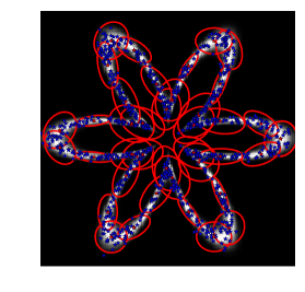
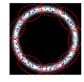
Proposal contours for the Flower target.
The -dimensional flower target is given by
This distribution concentrates around the -circle with a periodic perturbation (with amplitude and frequency ) in the first two dimensions. For , we obtain a band around the -circle, which we term the ring target. Figure 6 gives the contour plots of the MCMC Kameleon proposal distributions on two instances of the flower target.
Convergence statistics for the Banana target.
Figure 7 illustrates how the norm of the mean and quantile deviation (shown for -quantile) for the strongly twisted Banana target decrease as a function of the number of iterations. This shows that the trends observed in the main text persist along the evolution of the whole chain.
Appendix C Principal Components Proposals
An alternative approach to the standard adaptive Metropolis, discussed in Andrieu & Thoms (2008, Algorithm 8), is to extract principal eigenvalue-eigenvector pairs from the estimated covariance matrix and use the proposal that takes form of a mixture of one-dimensional random walks along the principal eigendirections
| (7) |
In other words, given the current chain state , the -th principal eigendirection is chosen with probability (choice is suggested), and the proposed point is
| (8) |
with . Note that each eigendirection may have a different scaling factor in addition to the scaling with the eigenvalue.
We can consider an analogous version of the update (8) performed in the RKHS
| (9) |
with principal eigenvalue-eigenfunction pairs . It is readily shown that the eigenfunctions lie in the subspace induced by , and that the coefficients vectors are proportional to the eigenvector of the centered kernel matrix , with normalization chosen so that (so that the eigenfunctions have the unit RKHS norm). Therefore, the update (9) has form
where . But are themselves the (unit norm) eigenvectors of as . Therefore, the appropriate scaling with eigenvalues is already included in the -coefficients, just like in the MCMC Kameleon, where the -coefficients are isotropic.
Now, we can construct the MCMC PCA-Kameleon by simply substituting -coefficients with , where is the selected eigendirection, and is the scaling factor associated to the -th eigendirection. We have the following steps:
-
1.
Perform eigendecomposition of to obtain the eigenvectors
-
2.
Draw
-
3.
-
4.
( normal in the original space)
Similarly as before, we can simplify the proposal by integrating out the scale of the moves in the RKHS.
Proposition 3.
.
Proof.
We start with
By substituting
we integrate out to obtain:
where . We can simplify the covariance using the Woodbury identity to obtain:
The claim follows after summing over the choice of the eigendirection (w.p. ).∎