Constraints on neutrino density and velocity isocurvature modes from WMAP-9 data
Abstract
We use WMAP 9-year and other CMB data to constrain cosmological models where the primordial perturbations have both an adiabatic and a (possibly correlated) neutrino density (NDI), neutrino velocity (NVI), or cold dark matter density (CDI) isocurvature component. For NDI and CDI we use both a phenomenological approach, where primordial perturbations are parametrized in terms of amplitudes at two scales, and a slow-roll two-field inflation approach, where slow-roll parameters are used as primary parameters. For NVI we use only the phenomenological approach, since it is difficult to imagine a connection with inflation. We find that in the NDI and NVI cases larger isocurvature fractions are allowed than in the corresponding models with CDI. For uncorrelated perturbations, the upper limit to the primordial NDI (NVI) fraction is 24% (20%) at and 28% (16%) at . For maximally correlated (anticorrelated) perturbations, the upper limit to the NDI fraction is 3.0% (0.9%). The nonadiabatic contribution to the CMB temperature variance can be as large as 10% (–13%) for the NDI (NVI) modes. Bayesian model comparison favors pure adiabatic initial mode over the mixed primordial adiabatic and NDI, NVI, or CDI perturbations. At best, the betting odds for a mixed model (uncorrelated NDI) are 1:3.4 compared to the pure adiabatic model. For the phenomenological generally correlated mixed models the odds are about 1:100, whereas the slow-roll approach leads to 1:13 (NDI) and 1:51 (CDI).
pacs:
98.70.Vc, 98.80.CqI Introduction
Cosmological models with cold dark matter isocurvature perturbations (CDI) were extensively studied in light of Wilkinson Microwave Anisotropy Probe (WMAP) seven-year data in Valiviita et al. (2012) both in a phenomenological and multi-field inflationary set-ups. Now we test within a similar framework what information the nine-year WMAP (WMAP-9) data Bennett et al. (2012); Larson et al. (2011) and other, smaller scale, cosmic microwave background (CMB) data Reichardt et al. (2009); Brown et al. (2009) give on possible deviations from adiabaticity, focusing on the less studied neutrino density (NDI) and velocity (NVI) isocurvature modes. For completeness we also update the analysis of the CDI mode. Recently, the CDI, NDI, and NVI modes were discussed in Ade et al. (2013a) in light of the Planck data, but only using a phenomenological approach and without simultaneously allowing for the possible tensor perturbation component.
Along with the adiabatic mode, the baryon density isocurvature (BDI), CDI, NDI and NVI modes are the only regular primordial scalar perturbation modes Bucher et al. (2000), others are either decaying modes or singular. The BDI and CDI modes are indistinguishable at the linear level in the CMB (see however Grin et al. (2013, 2011)) and the results for the CDI mode can easily be interpreted as constraints on the total matter density isocurvature.
We define the different perturbation modes using the five perturbation quantities: 1) the curvature perturbation in the comoving gauge, , 2) the cold dark matter entropy perturbation
| (1) |
3) the baryon entropy perturbation
| (2) |
4) the neutrino entropy perturbation
| (3) |
and 5) the relative neutrino heat flux Lewis (2011)
| (4) |
where the are density contrasts of the different energy components, the are velocity perturbation potentials, and stands for radiation, i.e., photons () and neutrinos (). The pure perturbation modes correspond to 4 of these 5 quantities vanishing initially (in the limit where conformal time ).
Thus in the adiabatic (or pure CDI, BDI, NDI, NVI) mode, initially only (or , , , ) .111Note that sometimes, for example in Langlois and van Tent (2012), these modes are defined in terms of , , , and instead, which leads to a different definition of the NDI mode, since if , then and can vanish initially, but in the limit . On the other hand, if , then and can vanish initially, but in the limit . The neutrino perturbation quantities are related by and , where is the neutrino energy density fraction. CAMB uses the definitions with respect to the total radiation, i.e., and Lewis (2011).
There is so far no evidence for a CDI, NDI, nor NVI perturbation component, and CMB temperature anisotropy observations require them to be subdominant compared to the adiabatic component Enqvist et al. (2000, 2002); Beltran et al. (2005a, b); Keskitalo et al. (2007); Trotta (2007); Seljak et al. (2006); Lewis (2006); Bean et al. (2006); Kawasaki and Sekiguchi (2008); Beltran (2008); Sollom et al. (2009); Valiviita and Giannantonio (2009); Castro et al. (2009); Li et al. (2011); Ade et al. (2013a).
We assume a power-law power spectrum for the primordial curvature and isocurvature perturbations and for their correlation. We also allow for tensor perturbations, which are a natural prediction of inflationary models. However, we allow only one isocurvature mode at a time, since the more general cases, where we have a mixture of several isocurvature modes in addition to the adiabatic and tensor modes, are quite intractable with the present data. In addition to the generally correlated perturbations, we study special cases with no correlation or with 100% correlation. Assuming spatially flat geometry of the Universe, we perform full parameter scans of this mixed (adiabatic and isocurvature) model, as well as the standard adiabatic CDM model. We present posterior probability densities of the standard cosmological parameters and the extra isocurvature parameters and report the Bayesian evidences for the models. These evidences give the betting odds for the pure adiabatic model against the various mixed (isocurvature) models.
We use two different approaches: 1) A phenomenological approach, where we make no reference to the origin of the primordial perturbations and just determine or constrain their amplitudes from the data, allowing the spectra of the adiabatic, isocurvature, and correlation components to be independent. 2) For the CDI and NDI modes, we also use a slow-roll two-field inflation approach, where we assume the perturbations were generated by quantum fluctuations during two-field inflation, and the spectral indices are determined by the slow-roll parameters at the time the cosmological scales exited the horizon during inflation. This approach forces the spectra to be nearly scale invariant, since we assume the magnitude of the slow roll parameters to be small.
The first approach is good for detecting non-adiabatic features in the data. If these were found, then a further investigation would be motivated. If not, then we can set an upper limit to the non-adiabaticity of the data. The second approach may give answers to questions directly related to inflation and inflationary potential.
We use the same notation as in Valiviita et al. (2012). A summary of the symbols can be found in Table I of Valiviita et al. (2012). In Sec. II we introduce our model and its phenomenological and inflationary parametrizations. In Sec. III we review two scenarios for generating the NDI mode. In Sec. IV we describe the data and sampling method. Secs. V and VI are devoted to the results. We summarize the main findings in Sec. VII and discuss why WMAP-9 leads to tighter constraints than the recent Planck data.
II The model
We assume that the primordial perturbation, here presented in Fourier space, is a superposition of the adiabatic mode (characterized by the comoving curvature perturbation ) and an isocurvature mode characterized by , where is either , , or . The power spectrum and its components are defined by the expectation value
| (5) |
Following Peiris et al. (2003); Valiviita and Muhonen (2003); Kurki-Suonio et al. (2005); Keskitalo et al. (2007); Kawasaki and Sekiguchi (2008); Valiviita and Giannantonio (2009) we divide into an uncorrelated part (“ar”) and a part fully correlated with (“as”), and assume power-law forms for the power spectra:
| (6) |
where
| (7) |
Since the spectral indices and are assumed constant (i.e. do not depend on ), the effective single adiabatic spectral index will depend on the scale (i.e., has running), in particular, if and differ a lot Valiviita and Muhonen (2003).
For the isocurvature and correlation we have
| (8) | |||||
| (9) |
where
| (10) |
We denote the values of power spectra at scale by , , and . In the following we choose three reference (i.e., pivot) scales
| (11) |
We further define the total primordial perturbation power
| (12) |
the primordial isocurvature fraction
| (13) |
and the ratio of the correlated adiabatic component to the total adiabatic power
| (14) |
so that
| (15) |
On the last line we defined the relative amplitude of the primordial correlation between the adiabatic and isocurvature perturbations, .
The total CMB temperature angular power spectrum can be written as
| (16) |
where the represent the different contributions to the angular power spectrum that would result from a corresponding primordial spectrum with unit amplitude at the pivot scale (see Kurki-Suonio et al. (2005)). comes from the primordial tensor perturbations.
The total non-adiabatic contribution to the CMB temperature variance,
| (17) | |||||
is our pivot-scale free measure of the non-adiabaticity.
Our sign convention for and is such that for NDI and NVI a positive primordial correlation leads to a positive contribution to the final spectrum, i.e., a positive primordial (or ) gives . In the case of CDI this is true in the Sachs-Wolfe region (at low multipoles), but at higher multipoles keeps changing its sign as a function of , although the primordial correlation does not change its sign as a function of in our model.
II.1 Phenomenological parametrization
The above model has six independent scalar perturbation parameters. In the amplitude parametrization we assign uniform priors to the following primary parameters:
| (18) |
As we assume power law spectra, the sign of correlation can not be a function of . Therefore the sign of has to be the same as that of . The background is described by the usual CDM background parameters, i.e., the physical baryon density, the physical CDM density, the sound horizon angle at last scattering , and the optical depth:
| (19) |
In addition, we include in the analysis the primordial tensor perturbations with a power law power spectrum
| (20) |
Their amplitude has been traditionally parametrized by the tensor-to-scalar ratio . In principle, in the phenomenological treatment the tensor perturbations would add two extra parameters, and the tensor spectral index . However, as no tensor nor isocurvature perturbations have been detected so far, allowing to be a free parameter would give us too many poorly constraint parameters to make this study feasible. As the focus of this paper are the isocurvature perturbations, we assume even in the phenomenological approach the first inflationary consistency relation which fixes , see, e.g., Lidsey et al. (1997); Bartolo et al. (2001a); Wands et al. (2002); Cortes and Liddle (2006); Kawasaki and Sekiguchi (2008). Therefore the tensor perturbations add only one extra free parameter while the tensor spectral index is a derived parameter given by the consistency relation . We impose also the second consistency relation Cortes et al. (2007); Cortes and Liddle (2006), which gives the running .
Assigning a uniform prior for and and using the first inflationary consistency relation, as described above, would lead to an unphysical prior on . Namely, the tensor spectral index would receive huge negative values whenever was near to one. This is against the very motivation of using the consistency relation, which was to force the tensor spectrum to follow the typical inflationary prediction of near scale invariance, . In addition, the large scale (low multipole) CMB data will not allow for such a huge tensor contribution. Hence, the use of the first consistency relation would artificially exclude any models where was near to one. (We will demonstrate this later in the end of Sec. V.1.) In order to avoid these problems, we will not parametrize the tensor power by , but instead by
| (21) |
for which we assign a uniform prior between and . When connecting the model to inflation, is the ratio of tensor to curvature perturbations generated at horizon exit, to the leading order in slow-roll parameters. So it reflects directly the inflationary physics, and hence a uniform prior on it is physically motivated. On the other hand, is a parameter directly related to observables. With our new definition the first consistency relation reads
| (22) |
which leads to a uniform prior on the derived parameter between and without being affected by the correlation parameter .
Furthermore, our new parametrization has an advantage when studying the fully (anti)correlated models, . In these special cases there is no tensor contribution. So, we can turn off tensors in CAMB and set the tensor parameters to constant values, and . However, in the “old parametrization” we cannot recover these special cases from the general case by taking the limit and , since this would correspond to . In the new parametrization the tensorless limit gives naturally and . So, although we do the special cases as separate MultiNest runs, we can also see the behavior of the posterior in the limit from our generally correlated runs.
II.2 Inflationary slow-roll parametrization
In the inflationary slow-roll approach we assume that during inflation there exists at least two “active” fields. The field space can be locally rotated so that the perturbations can be described by an adiabatic component, which is a perturbation in the direction of the background trajectory , and an “isocurvature” component which is a perturbation in the perpendicular direction . Now we can define four slow-roll parameters that are calculated from the inflationary potential at the time the interesting scale exits the horizon as follows:
| (23) |
From the slow-roll parameters we can determine the spectral indices and the tensor-to-scalar ratio at horizon exit, :
| (24) |
where the primordial correlation angle is defined by
| (25) |
with . The relations (24) are valid to first order in slow-roll parameters, see Byrnes and Wands (2006); Bartolo et al. (2001a); Wands et al. (2002); van Tent (2004); Peterson and Tegmark (2011) and note that, e.g., in Byrnes & Wands Byrnes and Wands (2006) stands for a scale-invariant spectrum whereas we have added the conventional 1 (except for tensors) and we use a different sign convention for and thus also for .
In the the slow-roll approach we have the same background parameters as in the phenomenological approach, Eq. (19), but the perturbations are parametrized by the four slow-roll parameters (three whose prior is uniform from to and with the prior range from to ), and . Note that unlike in the fully numerical treatments, see e.g. Norena et al. (2012), we can only allow small magnitudes for the slow-roll parameters, so that Eq. (24) is accurate enough. Our choice of prior ranges should guarantee that the second order corrections to are less than .
III Mechanisms that may produce neutrino isocurvature
There are various mechanisms that can produce (correlated) isocurvature and adiabatic perturbations, see, e.g., Refs. Choi et al. (2009); Hamazaki (2008); Di Marco et al. (2007); Lalak et al. (2007); Choi et al. (2007); Byrnes and Wands (2006); Rigopoulos et al. (2007); Bassett et al. (2006); Hattori and Yamamoto (2005); Di Marco and Finelli (2005); Parkinson et al. (2005); Gruzinov (2004); Bartolo et al. (2004); Vernizzi (2004); Lee and Fang (2004); van Tent (2004); Mazumdar and Postma (2003); Malik et al. (2003); Di Marco et al. (2003); Ashcroft et al. (2004); Bernardeau and Uzan (2002); Wands et al. (2002); Tsujikawa and Bassett (2002); Starobinsky et al. (2001); Bartolo et al. (2001a); Groot Nibbelink and van Tent (2002); Bartolo et al. (2001b); Hwang and Noh (2002, 2000); Gordon et al. (2001); Taylor and Berera (2000); Finelli and Brandenberger (2000); Liddle and Mazumdar (2000); Bassett et al. (2000); Pierpaoli et al. (1999); Langlois (1999); Felder et al. (1999); Perrotta and Baccigalupi (1999); Chiba et al. (1998); Nakamura and Stewart (1996); Polarski and Starobinsky (1994). The common ingredient of these models is that at least one extra degree of freedom is needed in addition to the one degree of freedom provided by the single-field slow-roll inflation, which can give rise to only the adiabatic mode. Multi-field inflationary models and curvaton/spectator field models are natural candidates for generating primordial CDI or NDI perturbations. In Valiviita et al. (2012) we reviewed several such scenarios focusing on the CDI case. Here we will provide examples of stimulating the NDI mode.
It has been suggested Lyth et al. (2003) (see also Gordon and Malik (2004); Kawasaki et al. (2012); Di Valentino et al. (2012)) that NDI might be generated from inhomogeneous lepton asymmetry in the context of the curvaton scenario. In the curvaton scenario the light curvaton field remains subdominant during inflation but may become important once the inflaton has decayed into radiation. This happens because once the Hubble parameter becomes smaller than the mass of the curvaton, the curvaton starts oscillating and behaves like dust and thus loses energy slower than the radiation fluid. This causes the perturbations in the curvaton to be transferred to the curvature perturbation,
| (26) |
where is evaluated at the time of curvaton decay. If the lepton number is generated before curvaton decay the NDI perturbation is
| (27) |
where is the neutrino asymmetry parameter.222The non-zero chemical potential of neutrinos affects the effective number of neutrino species by (28) Assuming the standard and the Big Bang nucleosynthesis (BBN) constraint , we find that the corrected number would be . Even as large as 0.2, would lead to quite a small correction, . Anyway, we checked that our NDI runs (see Sec. VI.2) led to virtually identical results with and . So, we can safely perform the analysis with the standard . Perturbations are fully anticorrelated and the isocurvature fraction is
| (29) |
BBN constrains Orito et al. (2002), which implies , too small to be observed.
If the lepton number is created directly from curvaton decay, however, the neutrino isocurvature perturbation is Lyth et al. (2003)
| (30) |
and the perturbations are fully correlated with isocurvature fraction
| (31) |
Now the isocurvature fraction can be significant if the curvaton decays sufficiently early. However, non-Gaussianity in the curvaton scenario is
| (32) |
which implies from the latest Planck 2 constraint Ade et al. (2013b). Eq. (31) gives largest when is the largest possible. Hence, saturating with the BBN constraint, the above result for leads to .
The NVI mode is more difficult to motivate theoretically because it would have to be generated after neutrino decoupling, and there are no proposed theoretical models to date. Thus we study the NVI mode only in the phenomenological set-up.
IV Data and sampling method
We employ the CMB temperature and polarization anisotropy data: WMAP-9 data Bennett et al. (2012), the Arcminute Cosmology Bolometer Array Receiver (ACBAR) data Reichardt et al. (2009), and QUEST at DASI (QUaD) data Brown et al. (2009) (QUEST stands for Q and U Extragalactic Survey Telescope, and DASI for Degree Angular Scale Interferometer). The additional CMB dataset are the same as in Valiviita et al. (2012) to make the comparison clear and in order to see whether there are significant differences between WMAP-7 and WMAP-9.
We sample the parameter space using the MultiNest nested sampling package Feroz et al. (2009); Mul , see also Skilling (2004); Mukherjee et al. (2006); Shaw et al. (2007); Feroz and Hobson (2008). It is easy to interface with CAMB/CosmoMC codes Lewis et al. (2000); Lewis and Bridle (2002) that we have modified to handle arbitrarily correlated mixtures of adiabatic and isocurvature perturbations.
V Results for the generally correlated mixed adiabatic and isocurvature models
In this section we let in the amplitude parametrization or and in the slow-roll parametrization to be free parameters, thus allowing for a general scale-dependent correlation amplitude between the adiabatic and one isocurvature mode (either CDI, NDI or NVI). These models have four extra parameters compared to the “standard” adiabatic CDM model.
V.1 Phenomenological approach — Amplitude parametrization for CDI, NDI and NVI
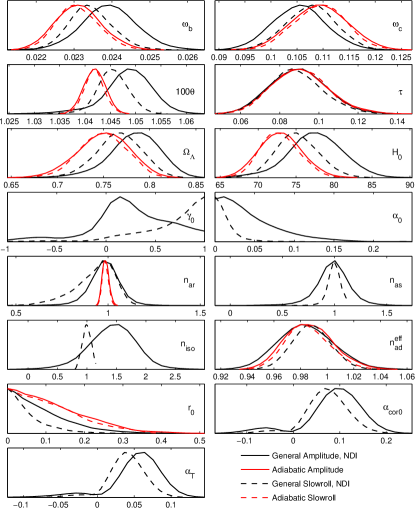
The marginalized 1-d posterior probability density functions (pdf) in the mixed adiabatic and isocurvature models (NDI, NVI, CDI) are compared to the pure adiabatic model in Fig. 1 (primary parameters) and Fig. 2 (selected derived parameters). In Appendix A we tabulate 68% or 95% confidence level (C.L.) intervals for selected parameters and the Bayesian evidence (see the third column of tables 1, 2 and 3 for the generally correlated mixed models).
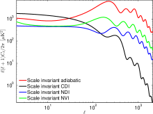
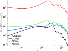
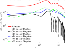
For the NDI and CDI modes a positive correlation333Recall our sign convention presented after Eq. (17). with the curvature perturbations is preferred by the data, whereas in case of the NVI mode, a negative correlation is preferred. This can be explained by the temperature angular power spectra of Fig. 3. In the left panel we plot the angular power spectra resulting from pure isocurvature or pure adiabatic scale-invariant primordial perturbations with the same background parameters. The CDI and NDI modes produce an acoustic peak that is to the right of the first acoustic peak of the adiabatic case, whereas the NVI mode leads to a peak that is slightly to the left. For a long time it has been known that in the CDI case the WMAP data prefer minimizing the CDI contribution everywhere Kurki-Suonio et al. (2005); Keskitalo et al. (2007); Valiviita and Giannantonio (2009); Valiviita et al. (2012). Since there is damping of the CDI mode compared to the adiabatic mode (see again the left panel of Fig. 3), the overall minimization of the isocurvature contribution is achieved by a relatively large . With WMAP-9 and other CMB data used in this paper, the median of the posterior pdf for CDI is (Fig. 2 and Table 3).
In the middle (right) panel of Fig. 3 we show a typical well-fitting adiabatic model and the isocurvature (non-adiabatic, i.e., isocurvature correlation) contributions of the well-fitting mixed adiabatic and isocurvature models. For these plots we used the median values of the 1-d pdf of each parameter. So, these curves are “representative” of the curves in the good-fit region. Compared to the correlation contribution, the actual isocurvature contribution is negligible. Therefore we focus on the right panel. For the CDI mode, as well as for the NDI mode, the correlation component would push the first acoustic peak toward the right compared to the pure adiabatic case, which fits the data very well. To push the peak back toward the left (in order to fit the data) we need in these models a larger sound horizon angle, see the solid black (NDI) and dashed black (CDI) pdfs for in Fig. 1. As explained, e.g., in Kurki-Suonio et al. (2005); Keskitalo et al. (2007); Valiviita and Giannantonio (2009); Valiviita et al. (2012) this leads to a larger Hubble parameter , a larger , and a smaller than in the pure adiabatic model, since we are studying models with a flat spatial geometry ().
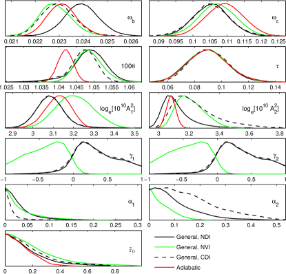
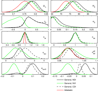
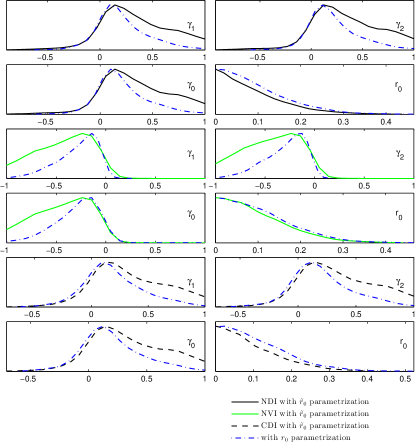
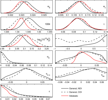
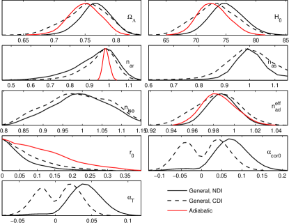
The phase of the NVI mode is very different from the NDI and CDI. Positively correlated NVI would tend to add power to the left side of the first adiabatic acoustic peak and to reduce the relative power on the right side of the peak. In the mixed model this would move the first acoustic peak to the left compared to the pure adiabatic model. However, a negative NVI correlation works in the opposite way, and hence leads to a very similar effect as the positive correlation in the NDI and CDI cases. Then the pdfs of the primary background parameters , , and (Fig. 1), as well as the derived parameters and (Fig. 2) are very similar in all the mixed models, whereas the pdfs of for the mixed NVI model are rough mirror images of those of the mixed NDI and CDI models.
The constraints on the primordial isocurvature fraction are tightest for the CDI on large scales (see in Fig. 1) and weakest on small scales (see ). This is reflected in the derived parameter in Fig. 2. Indeed, assuming that the data do not like any isocurvature contribution, the preferred order of the values of could have been guessed by seeing the left panel of Fig. 3. Nearly scale-invariant spectrum is preferred in the NVI case, since this type of NVI mode leads to roughly constant fractional isocurvature contribution over the whole range of acoustic peaks.
The primordial correlation amplitude describes best the primordial deviation from pure adiabaticity, unless the correlation parameter is (nearly) zero. We find at Mpc-1 a constraint for NDI, for NVI, and for CDI at 95% C.L. For the primordial isocurvature fraction the corresponding numbers are 0.14 (NDI), 0.10 (NVI), and 0.10 (CDI). The CMB data do not show any preference for the mixed models: all the posterior pdfs of the primordial isocurvature fraction peak at zero or very near to zero. The improvement of the of the best-fitting models compared to the adiabatic model does not exceed the number of extra parameters introduced by the isocurvature modes.
From Fig. 2 we see that a larger nonadiabatic contribution to the CMB temperature variance is allowed by the data in the case of the neutrino isocurvature modes than for the CDI mode. This is because the contribution from the neutrino modes is not as much off-phase from the adiabatic contribution (and the data agrees well with this adiabatic placement of the acoustic peaks), see Fig. 3. Another contributor to this result is that in the CDI case the correlation component keeps changing its sign as a function of multipole, whereas in the neutrino isocurvature cases has the same sign as the primordial correlation over the whole multipole range. Thus, in the CDI case, there are some cancellations in the summation over in Eq. (17). This may lead to a smaller non-adiabatic contribution to the total CMB temperature variance than to the individual multipoles in the CDI case. The 95% C.L. constraints are (NDI), (NVI), and (CDI). The apparent missing of the adiabatic case from the 95% C.L. interval of the NVI case is due to the very similar acoustic peak structures of the NVI and adiabatic modes. Thus the NVI mode is the most difficult to distinguish from the adiabatic one. However, as written above, the pdf of the primordial isocurvature fraction peaks at zero even in the NVI case.
Now we comment on the Bayesian evidences reported on the last lines of Tables 1, 2 and 3. The adiabatic model is favored. It has , whereas the mixed models (with general correlation) all have …. So the betting odds in favor of the pure adiabatic model against the mixed models are roughly .
Finally, in Fig. 4 we show the effect of our new parametrization on the posterior pdfs of and (which in the parametrization is a derived parameter). The constraints of are not much affected, but as we expected, in parametrization the values of are constrained by the data, not by the unphysical prior of the derived parameter (tensor spectral index). As a result our new constraints on are weaker than those presented in Valiviita et al. (2012) for the CDI case with WMAP-7 or those presented in Kawasaki and Sekiguchi (2008) for NDI, NVI, and CDI cases with WMAP-3 data. Naturally, the posterior pdfs of other parameters than or are also affected to some extent. For example, we obtain slightly tighter constraints on the isocurvature fraction in the new parametrization (since larger correlation fractions are allowed and hence a fixed leads to a larger non-adiabatic modification).
V.2 Two-field inflation approach — Slow-roll parametrization for NDI and CDI
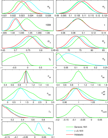
Fig. 5 shows marginalized 1-d posterior pdfs of the primary parameters in the slow-roll parametrization, and Fig. 6 the selected derived parameters. The medians of the pdfs and 68% or 95% C.L. intervals are provided in Appendix A in Tables 4 and 5 for the mixed NDI and CDI models. (As discussed earlier, the NVI mode is hard to think of as resulting from inflationary physics, hence we do not include it in our slow-roll analysis.)
The most significant difference from the previous subsection is that the slow-roll parametrization forces the power spectra, in particular the isocurvature and correlation spectra, to be nearly scale-invariant, see Eq. (24). In the CDI case the difference is most dramatic, since the phenomenological approach led to the median . For NDI the difference is smaller, since it gave the median . For NVI the slow-roll and phenomenological () approaches would be almost identical. In the slow-roll parametrization the CDI and NDI modes can significantly modify only the low- part of the spectrum, see the left panel of Fig. 3. We find tighter constraints than in the phenomenological approach: now , (NDI), and , (CDI).
A comparison of the posterior pdfs in amplitude and slow-roll parametrization for the NDI case is shown in Fig. 7. (A similar comparison for the CDI case can be found in Valiviita et al. (2012) with WMAP-7 data, or with WMAP-9 by comparing Figs. 1 and 2 to 5 and 6.) In both the NDI and CDI cases, the preferred values of most of the parameters in slow roll parametrization are between preferred values of the pure adiabatic case and the amplitude parametrization. The reason is that the near scale-invariance of the primordial isocurvature spectrum prevents any significant non-adiabatic contribution to the acoustic peak structure, thus leaving the high- part of angular power spectrum virtually “adiabatic”.
The data prefer positive correlation between the NDI and adiabatic mode, as happened also in the phenomenological case. The nearly scale-invariant NDI mode is able to modify the first acoustic peak almost in the same way as in the amplitude parametrization (with ) if the correlation fraction is large enough, compare the left and right panels of Fig. 3. Thus, in the slow-roll parametrization much larger correlation fractions are favored; the pdf of peaks at one — at the full correlation. The situation is very different for the CDI mode, see in Fig. 5. While positive correlation was clearly preferred in the amplitude parametrization (due to the effects on the first acoustic peak), now any correlation fraction between and is allowed. As the only effect of the correlated CDI in the slow-roll parametrization is to add or reduce some power at low-, which is dominated by cosmic variance, the data are insensitive to the sign of correlation. Thus, for example, the parameters and just reflect the uncertainty caused by the cosmic variance, and their pdf is almost symmetric about zero.
In particular in the NDI case, the tensor-to-scalar ratio, , is constrained tighter in the slow-roll parametrization, since the positive correlation adds power at low-. Thus there is less room for the tensor contribution which would also add power at low-.
Of the four slow-roll parameters only is well constrained in all studied cases, while the three are unconstrained or very poorly constrained, except in the adiabatic case. The constraint on does not come only from the tensor contribution. From the first line of Eq. (24) it is obvious that if was near to the upper bound of our chosen prior range, this would lead to too red-tilted adiabatic spectrum, which cannot be compensated by the blue-tilted isocurvature spectrum at high-, since the third line of Eq. (24) gives .
In the slow-roll parametrization the adiabatic model has , whereas the mixed models (with general correlation) have (NDI) and (CDI). So the betting odds in favor of the adiabatic model are 13 : 1 against NDI, and 51 : 1 against CDI. In particular, the mixed NDI case is not overwhelmingly disfavored by the Bayesian model comparison when the slow-roll approach is adopted.
VI Special cases
Now we study uncorrelated () and maximally correlated () or anticorrelated () cases. The uncorrelated model has only two extra parameters compared to the “standard” adiabatic CDM model. In the maximally correlated cases, in the amplitude parametrization, we make an extra assumption that the adiabatic and isocurvature spectra have the same shape, which further reduces the number of parameters by one, leading to only one extra parameter. In the slow-roll parametrization the same shape of spectra follows directly from the second and third lines of Eq. (24).
VI.1 Uncorrelated case for NDI, NVI, and CDI
In the uncorrelated case the spectrum is absent, so we have only nine independent parameters: the four background parameters
| (33) |
and five perturbation parameters
| (34) |
where
| (35) |
The primary perturbation parameters in the amplitude parametrization are
| (36) |
and in the slow-roll parametrization
| (37) |
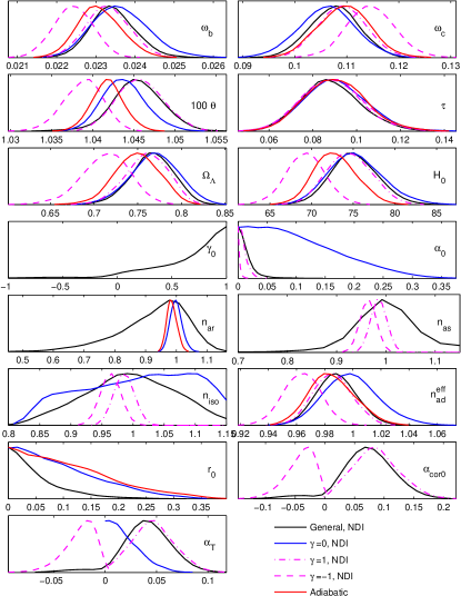
The marginalized 1-d posterior pdfs are indicated in Fig. 8 by solid blue curves for NDI and in Fig. 9 by solid cyan curves for NVI in the amplitude parametrization, and in Figs. 10 and 11 by solid blue curves for NDI in the slow-roll parametrization. (Again, we drop the NVI case from the slow-roll analysis as it is hard to motivate.) To allow for an easy comparison, we also plot the generally correlated and adiabatic cases presented in the previous section. Numerical results for the case are reported in the fourth columns of Tables 1 – 5.
On all scales in all cases the allowed primordial isocurvature fraction () is much larger in the uncorrelated case than in the generally correlated case or in the maximally correlated cases (studied in the next subsection). In the other models the main non-adiabatic effect comes from the correlation (whose amplitude is somewhere between the adiabatic and isocurvature contributions), but in the uncorrelated case the only disturbance to the adiabatic spectrum comes from the isocurvature itself. Thus rather large primordial fractions can be accommodated by the CMB data. However, since the isocurvature component is more off-phase from the adiabatic one than the correlation component, the allowed non-adiabatic contribution, , to the observed CMB temperature variance is smaller in all uncorrelated cases than in the general cases.
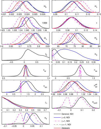
In the uncorrelated NDI and CDI cases the slow-roll parameters and are constrained equally well as in the adiabatic case, whereas remains unconstrained. A small isocurvature contribution at low- is allowed by the data (in particular due to cosmic variance) and the value of does not matter as long as the spectrum is nearly scale invariant (as it is due to our chosen priors of the slow-roll parameters). Since is simply 16 times , we find a tight constraint on the tensor-to-scalar ratio. Indeed, we find both in the uncorrelated NDI and CDI cases, while the pure adiabatic case leads to at 95% C.L. The tightening of the constraint on when allowing for the uncorrelated isocurvature component is natural, since adding power at low- eats room from the tensor contribution.
The betting odds in favor of the adiabatic model are 3.4, 16, 5.2, 3.5, and 16 : 1 when compared to the NDI (ampl. par.), NVI (ampl. par.), CDI (ampl. par.), NDI (slow-roll), CDI (slow-roll), respectively. Indeed, out of all models studied in this paper, the uncorrelated mixed NDI model in amplitude parametrization turns out to be least disfavored compared to the adiabatic model in terms of Bayesian model comparison.
VI.2 Maximally (anti)correlated NDI or CDI
In the fully correlated cases the spectrum is absent, and, following Valiviita et al. (2012), we assume there are no tensor perturbations. Moreover, according to Eq. (24), the two-field slow-roll inflation gives
| (38) |
No matter what is, these models lead to zero tensor contribution. Thus we can only constrain the combination , not and individually. Unlike in Valiviita et al. (2012), we assume also in the amplitude parametrization in order to make comparison to slow-roll results more straightforward and to have the same number of parameters in both parametrizations, which affects the Bayesian model comparison results.
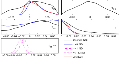
Therefore, we have only seven independent parameters: background parameters
| (39) |
and three perturbation parameters
| (40) |
Since (and the “ar” component is missing), the primordial isocurvature fraction is scale independent, .
The primary perturbation parameters in the amplitude parametrization are
| (41) |
and in the slow-roll parametrization
| (42) |
The marginalized 1-d posterior pdfs of the NDI case are indicated by the dashed magenta (, 100% anticorrelation) and dot-dashed magenta (, 100% correlation) curves in Fig. 8 for the amplitude parametrization, and in Figs. 10 and 11 for the slow-roll parametrization. The numerical values are tabulated in the fifth and sixth columns of Tables 1 (NDI) and 3 (CDI) in the amplitude parametrization, and in Tables 4 (NDI) and 5 (CDI) in the slow-roll parametrization. Note that we do not study the mixed NVI model with maximal (anti)correlation, since it is hard to think any physical mechanism that would lead to a correlation between NVI and adiabatic perturbations, since they may originate from very different epoch of the evolution of the universe.
In the amplitude parametrization, we obtain very tightly constrained isocurvature fraction for both the NDI and CDI cases, . The C.L. limits for NDI are and for and , respectively. Since the data force the adiabatic spectrum to be nearly scale invariant, and , we would expect very little difference to the slow-roll case, and indeed we find in the slow-roll parametrization very similar results, and for and , respectively. The reason for these tight constraints is that in the maximally correlated cases a fixed value of leads to much larger non-adiabatic contribution than in the partially correlated cases. As we would expect, in the cases where the maximal correlation has the same sign that was preferred in the general case, the constraints on and are very similar between the maximally correlated and generally correlated models.
The only “slow-roll parameter” of the maximally correlated cases, the combination , is well constrained.
The Bayesian evidences for the maximally correlated models are in all cases worse than for the uncorrelated models where we found the best evidences compared to the adiabatic model.
VII Discussion
We constrained the primordial fraction of all regular isocurvature modes, one at a time (matter density, neutrino density, and neutrino velocity isocurvature), as well as the non-adiabatic contribution to the observed CMB temperature variance. As the matter density (or CDI) mode has been extensively studied previously, our focus was on the neutrino isocurvature modes (NDI, NVI), but we also updated the constraints on CDI. Since primordial tensor perturbations are produced in typical inflationary models, we included tensor perturbations throughout the analysis.
In the phenomenological approach the power law spectra of the curvature and isocurvature mode, and the correlation between them, had independent amplitudes and tilts. This added four independent perturbation parameters to the standard adiabatic flat CDM scenario. If any clear non-adiabatic features were present in the CMB data used (WMAP-9, ACBAR, and QUaD), this approach should have found them. Neither frequentist nor Bayesian methods indicated any preference for any of the isocurvature modes: the CMB data set tight upper bounds on non-adiabatic contribution to the observed temperature variance.
Using Bayesian evidences calculated by MultiNest we established the betting odds for the models studied. For the generally correlated mixture of the adiabatic and one isocurvature mode (either NDI, NVI, or CDI) compared to the pure adiabatic primordial perturbation mode we found the odds to be as small as 1 : 100. However, in the special cases where we imposed restrictions to the correlation component, the betting odds were higher. In particular, for an uncorrelated mixed NDI model (which had two non-adiabatic extra parameters) the betting odds were 1 : 3.4 compared to the pure adiabatic model.
In the phenomenological set-up, with generally correlated mixed adiabatic and isocurvature perturbations, the tensor perturbations have been included at least in two different previous publications, in Kawasaki and Sekiguchi (2008) for NDI, NVI, and CDI, and in Valiviita et al. (2012) for CDI. In both of these, the first inflationary consistency relation was used in order to reduce the number of extra parameters. Namely, the tensor spectral index was determined from the consistency relation, , where was the tensor-to-scalar ratio (the ratio of tensor and total curvature perturbation power at the primordial time) and the correlation fraction. In both Kawasaki and Sekiguchi (2008) and Valiviita et al. (2012), assigning uniform priors on and (or ) led to “tight” constraints on . This was due to an unphysical prior of : whenever was near to one, the tensor spectral index was very negative. The huge tensor contribution thus induced was disfavored by the low- data. However, the original idea behind using the consistency relation was to obtain physically motivated (near to zero) values for as predicted by generic inflationary models, not huge negative values. In this paper we, for the first time, addressed these problems. We introduced the tensor-to-scalar ratio at horizon exit during inflation, . This is related to the above definition by . The inflationary consistency relation (derived to first order in slow-roll parameters) now read , and this led to a uniform prior on between and zero, avoiding unphysical values, and most importantly avoiding the interference of the use of consistency relation with the constraints on . The difference between the “old” and new approaches was presented in Fig. 4.
We studied the matter and neutrino density modes also in the two-field slow-roll inflation context, where we assumed uniform priors on the four first order slow-roll parameters (, , , ) and assumed their magnitude to be small, i.e., less than , so that the slow-roll approximation was accurate enough. The main difference to the phenomenological approach came from the fact that the choice of prior ranges of the slow-roll parameters restricted all the primordial spectra to be nearly scale invariant. (In the phenomenological approach the data favored blue tilted isocurvature spectra with spectral indices for NDI or for CDI, which in the slow-roll approach were excluded by the prior.)
In all those slow-roll cases, where tensor perturbations were produced, the posterior probability density of was much narrower than its prior. In the models with generally correlated primordial adiabatic and CDI or NDI mode, the constraint on was weaker than in the pure adiabatic model, but in the models with uncorrelated adiabatic and CDI or NDI mode the constraint on was tighter since the only possible effect (on the temperature angular power) of the nearly scale-invariant uncorrelated isocurvature component is to add power to the low multipoles, where also the tensor contribution would add power. Unlike , all three parameters were weakly constrained or unconstrained: since our slow-roll approach led to almost scale-invariant isocurvature and correlation spectra, the “non-adiabatic” modifications to appeared only in the low- region which is cosmic variance dominated and hence insensitive to the small tilts of the isocurvature and correlation components.
In Sec. III, assuming a curvaton-type model with inhomogeneous lepton asymmetry, and taking into account the big bang nucleosynthesis constraint on the neutrino asymmetry and the Planck constraint on non-Gaussianity (and converting this to a constraint of the curvaton inertia fraction at its decay time), we derived an upper limit for the primordial isocurvature fraction, , within this specific maximally correlated neutrino density isocurvature model. The direct constraint from the CMB, (see Sec. VI.2 for the constraints on NDI case in the amplitude parametrization), is weaker by a factor six.
In the recent literature, the CDI modes have been extensively contrasted against observations, but the observational constraints on neutrino isocurvature have been studied less, although theoretical work and future forecasts can be found in many publications, see e.g. Bucher et al. (2002, 2001); Kasanda et al. (2012); Zunckel et al. (2011); Langlois and van Tent (2012).
The most recent constraints on the phenomenological mixed CDI, NDI, and NVI models come from the Planck temperature anisotropy data, see Ade et al. (2013a). Perhaps surprisingly, the Planck constraints are weaker than what we find here with WMAP-9, ACBAR and QUaD. The Planck (our) upper bounds on the primordial isocurvature fraction on large scales, (in Ade et al. (2013a) called ), are 0.075 (0.045) for CDI, 0.27 (0.10) for NDI, and 0.18 (0.12) for NVI. The Planck parameter corresponds to our . The upper bounds on this are 0.39 (0.38) for CDI, 0.27 (0.27) for NDI, and 0.14 (0.13) for NVI. Finally, the 95% C.L. intervals for the non-adiabatic contribution to the observed CMB temperature variance (which is in Ade et al. (2013a)) are … (…) for CDI, … (…) for NDI, and … (…) for NVI.
The reason for such an unexpected difference between WMAP-9 and Planck is that the Planck data seem to prefer a negative correlation due to a relatively low power at low multipoles … compared to the higher multipoles. The adiabatic CDM model fits the acoustic peak structure of the Planck data with high precision, but even the best-fitting adiabatic model leads to more power at low- than seen in the data. This leads to a “demand” of some power-reducing mechanism at low-; a negatively correlated isocurvature can provide such an effect. This explains why the Planck constraints are weaker than the WMAP-9 constraints in particular at large scales (i.e., on ) and why Planck prefers negative correlation for all three cases (CDI, NDI, NVI), whereas WMAP-9 prefers a positive correlation in the CDI and NDI cases and a negative correlation in the NVI case (since with WMAP-9 the main non-adiabatic effects come from the first acoustic peak region).
Another crucial difference between WMAP-9 and Planck is that the Planck data prefer smaller and , and constrain the background parameters much tighter, thus leaving less freedom to play with their values. The WMAP-9 data preferred very large and in the phenomenological mixed models in order to compensate the shift of the first acoustic peak to right caused by the non-adiabatic component.
Some of the differences between Planck and our WMAP-9 results may come from the different parametrizations and assumptions. In Ade et al. (2013a) the curvature (i.e. adiabatic) spectrum was described by one power law, the isocurvature by one, and the correlation by one power law, which had a kink either at the low- or at the high- region to keep . Instead, we assumed two power-law components for the curvature perturbation, of which the other was fully correlated with the isocurvature power spectrum. This led our curvature spectrum to “auto-adjust” (run) in such a way that the above-mentioned mathematically necessary condition was always automatically satisfied without introducing kinks to any of the spectra. Moreover, we used the relative amplitudes and and logarithm of the “total” amplitudes as primary parameters, but in Ade et al. (2013a) the actual amplitudes of the three power spectra at two scales were primary parameters. We included also tensor perturbations in the analysis while in Ade et al. (2013a) the isocurvature analysis was done without tensor perturbations. However, based on Valiviita et al. (2012) we do not expect this to cause major differences.
In Valiviita et al. (2012) we studied the CDI mode in a similar set-up as NDI, NVI, and CDI here. We have checked the consistency of our new CDI results against the old ones. The differences can be traced to the following three points: different parametrization for the tensor-to-scalar ratio (in the phenomenological approach), different data, i.e., WMAP-9 versus WMAP-7, and an updated recombination code RECFAST in CAMB.
Acknowledgements.
This work was supported by the Academy of Finland grant 257989. This work was granted access to the HPC resources of CSC made available within the Distributed European Computing Initiative by the PRACE-2IP, receiving funding from the European Community’s Seventh Framework Programme (FP7/2007-2013) under grant agreement RI-283493. We thank the CSC - Scientific Computing Ltd (Finland) for computational resources. MS was supported by the Magnus Ehrnrooth Foundation, and SR by the Väisälä Foundation.References
- Valiviita et al. (2012) J. Valiviita, M. Savelainen, M. Talvitie, H. Kurki-Suonio, and S. Rusak, Astrophys.J. 753, 151 (2012), arXiv:1202.2852 [astro-ph.CO] .
- Bennett et al. (2012) C. Bennett et al. (WMAP Collaboration), (2012), arXiv:1212.5225 [astro-ph.CO] .
- Larson et al. (2011) D. Larson, J. Dunkley, G. Hinshaw, E. Komatsu, M. Nolta, et al., Astrophys.J.Suppl. 192, 16 (2011), arXiv:1001.4635 [astro-ph.CO] .
- Reichardt et al. (2009) C. L. Reichardt et al., Astrophys. J. 694, 1200 (2009), arXiv:0801.1491 [astro-ph] .
- Brown et al. (2009) M. Brown et al. (QUaD collaboration), Astrophys.J. 705, 978 (2009), arXiv:0906.1003 [astro-ph.CO] .
- Ade et al. (2013a) P. Ade et al. (Planck Collaboration), (2013a), arXiv:1303.5082 [astro-ph.CO] .
- Bucher et al. (2000) M. Bucher, K. Moodley, and N. Turok, Phys. Rev. D62, 083508 (2000), arXiv:astro-ph/9904231 .
- Grin et al. (2013) D. Grin, D. Hanson, G. Holder, O. Doré, and M. Kamionkowski, (2013), arXiv:1306.4319 [astro-ph.CO] .
- Grin et al. (2011) D. Grin, O. Doré, and M. Kamionkowski, Phys.Rev. D84, 123003 (2011), arXiv:1107.5047 [astro-ph.CO] .
-
Lewis (2011)
A. Lewis, “Camb notes,”
(2011),
http://cosmologist.info/notes/CAMB.pdf. - Langlois and van Tent (2012) D. Langlois and B. van Tent, JCAP 1207, 040 (2012), arXiv:1204.5042 [astro-ph.CO] .
- Enqvist et al. (2000) K. Enqvist, H. Kurki-Suonio, and J. Valiviita, Phys. Rev. D62, 103003 (2000), arXiv:astro-ph/0006429 .
- Enqvist et al. (2002) K. Enqvist, H. Kurki-Suonio, and J. Valiviita, Phys. Rev. D65, 043002 (2002), arXiv:astro-ph/0108422 .
- Beltran et al. (2005a) M. Beltran, J. Garcia-Bellido, J. Lesgourgues, A. R. Liddle, and A. Slosar, Phys. Rev. D71, 063532 (2005a), arXiv:astro-ph/0501477 .
- Beltran et al. (2005b) M. Beltran, J. Garcia-Bellido, J. Lesgourgues, and M. Viel, Phys. Rev. D72, 103515 (2005b), arXiv:astro-ph/0509209 .
- Keskitalo et al. (2007) R. Keskitalo, H. Kurki-Suonio, V. Muhonen, and J. Valiviita, JCAP 0709, 008 (2007), arXiv:astro-ph/0611917 .
- Trotta (2007) R. Trotta, Mon. Not. Roy. Astron. Soc. Lett. 375, L26 (2007), arXiv:astro-ph/0608116 .
- Seljak et al. (2006) U. Seljak, A. Slosar, and P. McDonald, JCAP 0610, 014 (2006), arXiv:astro-ph/0604335 .
- Lewis (2006) A. Lewis, (2006), arXiv:astro-ph/0603753 .
- Bean et al. (2006) R. Bean, J. Dunkley, and E. Pierpaoli, Phys. Rev. D74, 063503 (2006), arXiv:astro-ph/0606685 .
- Kawasaki and Sekiguchi (2008) M. Kawasaki and T. Sekiguchi, Prog. Theor. Phys. 120, 995 (2008), arXiv:0705.2853 [astro-ph] .
- Beltran (2008) M. Beltran, Phys. Rev. D78, 023530 (2008), arXiv:0804.1097 [astro-ph] .
- Sollom et al. (2009) I. Sollom, A. Challinor, and M. P. Hobson, Phys. Rev. D79, 123521 (2009), arXiv:0903.5257 [astro-ph.CO] .
- Valiviita and Giannantonio (2009) J. Valiviita and T. Giannantonio, Phys.Rev. D80, 123516 (2009), arXiv:0909.5190 [astro-ph.CO] .
- Castro et al. (2009) P. Castro et al. (QUaD collaboration), Astrophys.J. 701, 857 (2009), arXiv:0901.0810 [astro-ph.CO] .
- Li et al. (2011) H. Li, J. Liu, J.-Q. Xia, and Y.-F. Cai, Phys.Rev. D83, 123517 (2011), arXiv:1012.2511 [astro-ph.CO] .
- Peiris et al. (2003) H. Peiris et al. (WMAP Collaboration), Astrophys.J.Suppl. 148, 213 (2003), arXiv:astro-ph/0302225 [astro-ph] .
- Valiviita and Muhonen (2003) J. Valiviita and V. Muhonen, Phys. Rev. Lett. 91, 131302 (2003), arXiv:astro-ph/0304175 .
- Kurki-Suonio et al. (2005) H. Kurki-Suonio, V. Muhonen, and J. Valiviita, Phys. Rev. D71, 063005 (2005), arXiv:astro-ph/0412439 .
- Lidsey et al. (1997) J. E. Lidsey, A. R. Liddle, E. W. Kolb, E. J. Copeland, T. Barreiro, et al., Rev.Mod.Phys. 69, 373 (1997), arXiv:astro-ph/9508078 [astro-ph] .
- Bartolo et al. (2001a) N. Bartolo, S. Matarrese, and A. Riotto, Phys. Rev. D64, 123504 (2001a), arXiv:astro-ph/0107502 .
- Wands et al. (2002) D. Wands, N. Bartolo, S. Matarrese, and A. Riotto, Phys. Rev. D66, 043520 (2002), arXiv:astro-ph/0205253 .
- Cortes and Liddle (2006) M. Cortes and A. R. Liddle, Phys. Rev. D73, 083523 (2006), arXiv:astro-ph/0603016 .
- Cortes et al. (2007) M. Cortes, A. R. Liddle, and P. Mukherjee, Phys. Rev. D75, 083520 (2007), arXiv:astro-ph/0702170 .
- Byrnes and Wands (2006) C. T. Byrnes and D. Wands, Phys. Rev. D74, 043529 (2006), arXiv:astro-ph/0605679 .
- van Tent (2004) B. van Tent, Class.Quant.Grav. 21, 349 (2004), arXiv:astro-ph/0307048 [astro-ph] .
- Peterson and Tegmark (2011) C. M. Peterson and M. Tegmark, Phys.Rev. D83, 023522 (2011), arXiv:1005.4056 [astro-ph.CO] .
- Norena et al. (2012) J. Norena, C. Wagner, L. Verde, H. V. Peiris, and R. Easther, Phys.Rev. D86, 023505 (2012), arXiv:1202.0304 [astro-ph.CO] .
- Choi et al. (2009) K.-Y. Choi, J.-O. Gong, and D. Jeong, JCAP 0902, 032 (2009), arXiv:0810.2299 [hep-ph] .
- Hamazaki (2008) T. Hamazaki, Nucl. Phys. B791, 20 (2008), arXiv:0711.2954 [astro-ph] .
- Di Marco et al. (2007) F. Di Marco, F. Finelli, and A. Gruppuso, Phys. Rev. D76, 043530 (2007), arXiv:0705.2185 [astro-ph] .
- Lalak et al. (2007) Z. Lalak, D. Langlois, S. Pokorski, and K. Turzynski, JCAP 0707, 014 (2007), arXiv:0704.0212 [hep-th] .
- Choi et al. (2007) K.-Y. Choi, L. M. H. Hall, and C. van de Bruck, JCAP 0702, 029 (2007), arXiv:astro-ph/0701247 .
- Rigopoulos et al. (2007) G. I. Rigopoulos, E. P. S. Shellard, and B. J. W. van Tent, Phys. Rev. D76, 083512 (2007), arXiv:astro-ph/0511041 .
- Bassett et al. (2006) B. A. Bassett, S. Tsujikawa, and D. Wands, Rev. Mod. Phys. 78, 537 (2006), arXiv:astro-ph/0507632 .
- Hattori and Yamamoto (2005) T. Hattori and K. Yamamoto, JCAP 0507, 005 (2005), arXiv:astro-ph/0506373 .
- Di Marco and Finelli (2005) F. Di Marco and F. Finelli, Phys. Rev. D71, 123502 (2005), arXiv:astro-ph/0505198 .
- Parkinson et al. (2005) D. Parkinson, S. Tsujikawa, B. A. Bassett, and L. Amendola, Phys. Rev. D71, 063524 (2005), arXiv:astro-ph/0409071 .
- Gruzinov (2004) A. Gruzinov, (2004), arXiv:astro-ph/0401407 .
- Bartolo et al. (2004) N. Bartolo, P. S. Corasaniti, A. R. Liddle, and M. Malquarti, Phys. Rev. D70, 043532 (2004), arXiv:astro-ph/0311503 .
- Vernizzi (2004) F. Vernizzi, Phys. Rev. D69, 083526 (2004), arXiv:astro-ph/0311167 .
- Lee and Fang (2004) W. Lee and L.-Z. Fang, Phys. Rev. D69, 023514 (2004), arXiv:astro-ph/0310856 .
- Mazumdar and Postma (2003) A. Mazumdar and M. Postma, Phys. Lett. B573, 5 (2003), arXiv:astro-ph/0306509 .
- Malik et al. (2003) K. A. Malik, D. Wands, and C. Ungarelli, Phys. Rev. D67, 063516 (2003), arXiv:astro-ph/0211602 .
- Di Marco et al. (2003) F. Di Marco, F. Finelli, and R. Brandenberger, Phys. Rev. D67, 063512 (2003), arXiv:astro-ph/0211276 .
- Ashcroft et al. (2004) P. R. Ashcroft, C. van de Bruck, and A. C. Davis, Phys. Rev. D69, 083516 (2004), arXiv:astro-ph/0210597 .
- Bernardeau and Uzan (2002) F. Bernardeau and J.-P. Uzan, Phys. Rev. D66, 103506 (2002), arXiv:hep-ph/0207295 .
- Tsujikawa and Bassett (2002) S. Tsujikawa and B. A. Bassett, Phys. Lett. B536, 9 (2002), arXiv:astro-ph/0204031 .
- Starobinsky et al. (2001) A. A. Starobinsky, S. Tsujikawa, and J. Yokoyama, Nucl. Phys. B610, 383 (2001), arXiv:astro-ph/0107555 .
- Groot Nibbelink and van Tent (2002) S. Groot Nibbelink and B. J. W. van Tent, Class. Quant. Grav. 19, 613 (2002), arXiv:hep-ph/0107272 .
- Bartolo et al. (2001b) N. Bartolo, S. Matarrese, and A. Riotto, Phys. Rev. D64, 083514 (2001b), arXiv:astro-ph/0106022 .
- Hwang and Noh (2002) J.-c. Hwang and H. Noh, Class. Quant. Grav. 19, 527 (2002), arXiv:astro-ph/0103244 .
- Hwang and Noh (2000) J.-c. Hwang and H. Noh, Phys. Lett. B495, 277 (2000), arXiv:astro-ph/0009268 .
- Gordon et al. (2001) C. Gordon, D. Wands, B. A. Bassett, and R. Maartens, Phys. Rev. D63, 023506 (2001), arXiv:astro-ph/0009131 .
- Taylor and Berera (2000) A. N. Taylor and A. Berera, Phys. Rev. D62, 083517 (2000), arXiv:astro-ph/0006077 .
- Finelli and Brandenberger (2000) F. Finelli and R. H. Brandenberger, Phys. Rev. D62, 083502 (2000), arXiv:hep-ph/0003172 .
- Liddle and Mazumdar (2000) A. R. Liddle and A. Mazumdar, Phys. Rev. D61, 123507 (2000), arXiv:astro-ph/9912349 .
- Bassett et al. (2000) B. A. Bassett, C. Gordon, R. Maartens, and D. I. Kaiser, Phys. Rev. D61, 061302 (2000), arXiv:hep-ph/9909482 .
- Pierpaoli et al. (1999) E. Pierpaoli, J. Garcia-Bellido, and S. Borgani, JHEP 10, 015 (1999), arXiv:hep-ph/9909420 .
- Langlois (1999) D. Langlois, Phys. Rev. D59, 123512 (1999), arXiv:astro-ph/9906080 .
- Felder et al. (1999) G. N. Felder, L. Kofman, and A. D. Linde, Phys. Rev. D60, 103505 (1999), arXiv:hep-ph/9903350 .
- Perrotta and Baccigalupi (1999) F. Perrotta and C. Baccigalupi, Phys. Rev. D59, 123508 (1999), arXiv:astro-ph/9811156 .
- Chiba et al. (1998) T. Chiba, N. Sugiyama, and J. Yokoyama, Nucl. Phys. B530, 304 (1998), arXiv:gr-qc/9708030 .
- Nakamura and Stewart (1996) T. T. Nakamura and E. D. Stewart, Phys. Lett. B381, 413 (1996), arXiv:astro-ph/9604103 .
- Polarski and Starobinsky (1994) D. Polarski and A. A. Starobinsky, Phys. Rev. D50, 6123 (1994), arXiv:astro-ph/9404061 .
- Lyth et al. (2003) D. H. Lyth, C. Ungarelli, and D. Wands, Phys. Rev. D67, 023503 (2003), arXiv:astro-ph/0208055 .
- Gordon and Malik (2004) C. Gordon and K. A. Malik, Phys. Rev. D69, 063508 (2004), arXiv:astro-ph/0311102 .
- Kawasaki et al. (2012) M. Kawasaki, K. Miyamoto, K. Nakayama, and T. Sekiguchi, JCAP 1202, 022 (2012), arXiv:1107.4962 [astro-ph.CO] .
- Di Valentino et al. (2012) E. Di Valentino, M. Lattanzi, G. Mangano, A. Melchiorri, and P. Serpico, Phys.Rev. D85, 043511 (2012), arXiv:1111.3810 [astro-ph.CO] .
- Orito et al. (2002) M. Orito, T. Kajino, G. Mathews, and Y. Wang, Phys.Rev. D65, 123504 (2002), arXiv:astro-ph/0203352 [astro-ph] .
- Ade et al. (2013b) P. Ade et al. (Planck Collaboration), (2013b), arXiv:1303.5084 [astro-ph.CO] .
- Feroz et al. (2009) F. Feroz, M. Hobson, and M. Bridges, Mon.Not.Roy.Astron.Soc. 398, 1601 (2009), arXiv:0809.3437 [astro-ph] .
- (83) http://ccpforge.cse.rl.ac.uk/gf/project/multinest/.
- Skilling (2004) J. Skilling, AIP conference proceedings of the 24th international workshop on Bayesian inference and maximum entropy methods in science and engineering (2004).
- Mukherjee et al. (2006) P. Mukherjee, D. Parkinson, and A. R. Liddle, Astrophys. J. 638, L51 (2006), arXiv:astro-ph/0508461 .
- Shaw et al. (2007) R. Shaw, M. Bridges, and M. P. Hobson, Mon. Not. Roy. Astron. Soc. 378, 1365 (2007), arXiv:astro-ph/0701867 .
- Feroz and Hobson (2008) F. Feroz and M. Hobson, Mon.Not.Roy.Astron.Soc. 384, 449 (2008), arXiv:0704.3704 [astro-ph] .
- Lewis et al. (2000) A. Lewis, A. Challinor, and A. Lasenby, Astrophys. J. 538, 473 (2000), astro-ph/9911177 .
- Lewis and Bridle (2002) A. Lewis and S. Bridle, Phys. Rev. D66, 103511 (2002), astro-ph/0205436 .
- Bucher et al. (2002) M. Bucher, K. Moodley, and N. Turok, Phys. Rev. D66, 023528 (2002), arXiv:astro-ph/0007360 .
- Bucher et al. (2001) M. Bucher, K. Moodley, and N. Turok, Phys. Rev. Lett. 87, 191301 (2001), arXiv:astro-ph/0012141 .
- Kasanda et al. (2012) S. M. Kasanda, C. Zunckel, K. Moodley, B. Bassett, and P. Okouma, JCAP 1207, 021 (2012), arXiv:1111.2572 [astro-ph.CO] .
- Zunckel et al. (2011) C. Zunckel, P. Okouma, S. Kasanda, K. Moodley, and B. Bassett, Phys.Lett. B696, 433 (2011), arXiv:1006.4687 [astro-ph.CO] .
Appendix A Tables
| Parameter | C.L | Mixed NDI, general corr. | Mixed NDI, | Mixed NDI, | Mixed NDI, | Adiabatic |
| 68% | 0.0239 (0.0233, 0.0246) | 0.0239 (0.0232, 0.0247) | 0.0233 (0.0227, 0.0238) | 0.0224 (0.0219, 0.0229) | 0.0231 (0.0225, 0.0237) | |
| 68% | 0.1054 (0.1004, 0.1104) | 0.1049 (0.0995, 0.1102) | 0.1094 (0.1048, 0.1140) | 0.1145 (0.1102, 0.1191) | 0.1093 (0.1040, 0.1146) | |
| 68% | 1.0488 (1.0447, 1.0526) | 1.0452 (1.0425, 1.0482) | 1.0457 (1.0428, 1.0486) | 1.0389 (1.0364, 1.0411) | 1.0419 (1.0398, 1.0440) | |
| 68% | 0.0896 (0.0753, 0.1035) | 0.0911 (0.0776, 0.1065) | 0.0872 (0.0746, 0.1011) | 0.0884 (0.0756, 0.1023) | 0.0899 (0.0757, 0.1045) | |
| 68% | 0.7852 (0.7586, 0.8090) | 0.7800 (0.7525, 0.8070) | 0.7602 (0.7346, 0.7835) | 0.7147 (0.6865, 0.7388) | 0.7508 (0.7221, 0.7769) | |
| 68% | 77.56 (74.31, 81.01) | 76.49 (73.35, 80.16) | 74.35 (71.69, 77.11) | 69.28 (67.02, 71.47) | 72.95 (70.27, 75.69) | |
| 68% | 3.0713 (3.0260, 3.1323) | 3.2032 (3.1360, 3.2840) | 3.0717 (3.0342, 3.1120) | 3.1649 (3.1300, 3.2067) | 3.1038 (3.0641, 3.1422) | |
| 68% | 0.9835 (0.9640, 1.0042) | 0.9997 (0.9811, 1.0204) | 0.9850 (0.9718, 0.9992) | 0.9638 (0.9509, 0.9769) | 0.9859 (0.9685, 1.0041) | |
| 95% | -0.1137 | |||||
| 95% | -0.0894 | |||||
| 95% | 0.0980 | 0.2421 | 0.0303 | 0.0093 | ||
| 95% | 0.2713 | 0.4003 | 0.0303 | 0.0093 | ||
| 95% | 0.4751 | 0.2866 | 0.3334 | |||
| 95% | -0.1004 | |||||
| 95% | 0.1414 | 0.2816 | 0.0303 | 0.0093 | ||
| 95% | 0.9846 (0.8025, 1.1361) | 0.9997 (0.9651, 1.0427) | 0.9859 (0.9545, 1.0236) | |||
| 95% | 0.9837 (0.6240, 1.2896) | 0.9850 (0.9593, 1.0116) | 0.9638 (0.9377, 0.9889) | |||
| 95% | 1.4508 (0.5678, 2.1718) | 1.2465 (0.6096, 1.8885) | 0.9850 (0.9593, 1.0116) | 0.9638 (0.9377, 0.9889) | ||
| 95% | 0.2414 | 0.2866 | 0.3334 | |||
| 95% | 0.0961 (-0.0824, 0.1808) | 0.0846 (0.0184, 0.1713) | -0.0389 (-0.0960, -0.0067) | |||
| 95% | 0.0580 (-0.0486, 0.1028) | 0.0531 | 0.0462 (0.0104, 0.0916) | -0.0230 (-0.0593, -0.0039) | ||
| 3905.78 | 3902.38 | 3902.73 | 3905.35 | 3901.17 | ||
| 4.6 | 1.2 | 1.6 | 4.2 | 0 | ||
| 100 | 3.4 | 4.8 | 65 | 1 |
| Parameter | C.L | Mixed NVI, general corr. | NVI, | Adiabatic |
| 68% | 0.0228 (0.0222, 0.0235) | 0.0238 (0.0231, 0.0245) | 0.0231 (0.0225, 0.0237) | |
| 68% | 0.1071 (0.1020, 0.1122) | 0.1075 (0.1024, 0.1126) | 0.1093 (0.1040, 0.1146) | |
| 68% | 1.0484 (1.0451, 1.0521) | 1.0412 (1.0390, 1.0433) | 1.0419 (1.0398, 1.0440) | |
| 68% | 0.0898 (0.0760, 0.1040) | 0.0893 (0.0765, 0.1041) | 0.0899 (0.0757, 0.1045) | |
| 68% | 0.7744 (0.7482, 0.7984) | 0.7596 (0.7326, 0.7840) | 0.7508 (0.7221, 0.7769) | |
| 68% | 75.89 (73.05, 78.85) | 73.87 (71.33, 76.70) | 72.95 (70.27, 75.69) | |
| 68% | 3.1895 (3.1399, 3.2402) | 3.1462 (3.1005, 3.1930) | 3.1038 (3.0641, 3.1422) | |
| 68% | 0.9948 (0.9680, 1.0265) | 0.9958 (0.9777, 1.0171) | 0.9859 (0.9685, 1.0041) | |
| 95% | -0.0588 | |||
| 95% | -0.0604 | |||
| 95% | 0.1245 | 0.1961 | ||
| 95% | 0.1349 | 0.1976 | ||
| 95% | 0.6213 | 0.3088 | 0.3334 | |
| 95% | -0.0637 | |||
| 95% | 0.0997 | 0.1617 | ||
| 95% | 0.9935 (0.7785, 1.1985) | 0.9958 (0.9607, 1.0390) | 0.9859 (0.9545, 1.0236) | |
| 95% | 1.0009 (0.7213, 1.3083) | |||
| 95% | 1.1454 (0.0329, 2.4865) | 1.0528 (0.4302, 1.7779) | ||
| 95% | 0.2489 | 0.3088 | 0.3334 | |
| 95% | -0.0907 (-0.1636, -0.0333) | |||
| 95% | -0.0635 (-0.1267, -0.0091) | 0.0576 | ||
| 3905.57 | 3903.96 | 3901.17 | ||
| 4.4 | 2.8 | 0 | ||
| 81 | 16 | 1 |
| Parameter | C.L | Mixed CDI, general corr. | Mixed CDI, | Mixed CDI, | Mixed CDI, | Adiabatic |
| 68% | 0.0229 (0.0223, 0.0236) | 0.0237 (0.0230, 0.0244) | 0.0230 (0.0225, 0.0235) | 0.0225 (0.0221, 0.0230) | 0.0231 (0.0225, 0.0237) | |
| 68% | 0.1052 (0.1002, 0.1105) | 0.1062 (0.1007, 0.1113) | 0.1079 (0.1030, 0.1126) | 0.1162 (0.1113, 0.1212) | 0.1093 (0.1040, 0.1146) | |
| 68% | 1.0472 (1.0435, 1.0505) | 1.0436 (1.0415, 1.0459) | 1.0438 (1.0415, 1.0462) | 1.0391 (1.0370, 1.0412) | 1.0419 (1.0398, 1.0440) | |
| 68% | 0.0906 (0.0772, 0.1046) | 0.0922 (0.0790, 0.1067) | 0.0866 (0.0741, 0.1007) | 0.0903 (0.0764, 0.1046) | 0.0899 (0.0757, 0.1045) | |
| 68% | 0.7798 (0.7526, 0.8029) | 0.7700 (0.7430, 0.7976) | 0.7611 (0.7366, 0.7849) | 0.7076 (0.6768, 0.7342) | 0.7508 (0.7221, 0.7769) | |
| 68% | 76.24 (73.26, 79.26) | 75.16 (72.40, 78.60) | 74.02 (71.59, 76.67) | 68.85 (66.59, 71.17) | 72.95 (70.27, 75.69) | |
| 68% | 3.0931 (3.0540, 3.1404) | 3.1725 (3.1211, 3.2281) | 3.0859 (3.0498, 3.1223) | 3.1689 (3.1316, 3.2074) | 3.1038 (3.0641, 3.1422) | |
| 68% | 0.9961 (0.9788, 1.0149) | 1.0030 (0.9839, 1.0261) | 0.9902 (0.9751, 1.0064) | 0.9575 (0.9430, 0.9712) | 0.9859 (0.9685, 1.0041) | |
| 95% | -0.1275 | |||||
| 95% | -0.1042 | |||||
| 95% | 0.0454 | 0.1114 | 0.0148 | 0.0073 | ||
| 95% | 0.3815 | 0.5012 | 0.0148 | 0.0073 | ||
| 95% | 0.5238 | 0.2925 | 0.3334 | |||
| 95% | -0.1126 | |||||
| 95% | 0.0955 | 0.2110 | 0.0148 | 0.0073 | ||
| 95% | 0.9964 (0.8057, 1.1627) | 1.0030 (0.9673, 1.0506) | 0.9859 (0.9545, 1.0236) | |||
| 95% | 0.9995 (0.6086, 1.3376) | 0.9902 (0.9611, 1.0218) | 0.9575 (0.9284, 0.9845) | |||
| 95% | 2.0523 (0.8075, 3.3592) | 1.7338 (0.9795, 2.7873) | 0.9902 (0.9611, 1.0218) | 0.9575 (0.9284, 0.9845) | ||
| 95% | 0.2571 | 0.2925 | 0.3334 | |||
| 95% | 0.0747 (-0.0770, 0.1499) | 0.0531 (0.0100, 0.1206) | -0.0368 (-0.0852, -0.0063) | |||
| 95% | 0.0209 (-0.0295, 0.0467) | 0.0358 | 0.0272 (0.0055, 0.0582) | -0.0214 (-0.0532, -0.0035) | ||
| 3905.93 | 3902.82 | 3904.71 | 3905.49 | 3901.17 | ||
| 4.8 | 1.7 | 3.5 | 4.3 | 0 | ||
| 117 | 5.2 | 34 | 75 | 1 |
| Parameter | C.L. | Mixed NDI, gen. corr. | Mixed NDI, | Mixed NDI, | Mixed NDI, | Adiabatic |
| 68% | 0.0234 (0.0229, 0.0240) | 0.0236 (0.0229, 0.0243) | 0.0233 (0.0228, 0.0239) | 0.0224 (0.0219, 0.0229) | 0.0231 (0.0226, 0.0236) | |
| 68% | 0.1077 (0.1030, 0.1122) | 0.1064 (0.1010, 0.1114) | 0.1092 (0.1046, 0.1136) | 0.1145 (0.1102, 0.1190) | 0.1095 (0.1045, 0.1142) | |
| 68% | 1.0454 (1.0428, 1.0484) | 1.0437 (1.0413, 1.0464) | 1.0457 (1.0431, 1.0486) | 1.0390 (1.0365, 1.0411) | 1.0418 (1.0400, 1.0437) | |
| 68% | 0.0876 (0.0752, 0.1014) | 0.0901 (0.0768, 0.1041) | 0.0884 (0.0749, 0.1014) | 0.0891 (0.0755, 0.1025) | 0.0899 (0.0763, 0.1034) | |
| 68% | 3.0686 (3.0312, 3.1081) | 3.1739 (3.1167, 3.2499) | 3.0710 (3.0355, 3.1098) | 3.1663 (3.1307, 3.2057) | 3.1059 (3.0690, 3.1409) | |
| 68% | 0.7669 (0.7427, 0.7905) | 0.7699 (0.7427, 0.7966) | 0.7611 (0.7364, 0.7847) | 0.7151 (0.6865, 0.7397) | 0.7495 (0.7238, 0.7750) | |
| 68% | 75.02 (72.46, 77.89) | 75.13 (72.19, 78.48) | 74.47 (71.84, 77.26) | 69.33 (67.06, 71.53) | 72.75 (70.40, 75.36) | |
| 68% | 0.9879 (0.9742, 1.0026) | 0.9982 (0.9805, 1.0178) | 0.9853 (0.9720, 0.9990) | 0.9639 (0.9509, 0.9766) | 0.9843 (0.9697, 1.0021) | |
| 95% | -0.3178 | |||||
| 95% | 0.0568 | 0.2482 | 0.0280 | 0.0104 | ||
| 95% | p.r. | 0.0146 (-0.0129, 0.0641) | 0.0102 (-0.0175, 0.0637) | |||
| 95% | p.r. | |||||
| 95% | p.r. | p.r. | ||||
| 95% | 0.0570 | 0.0152 | 0.0193 | |||
| 95% | -0.0073 (-0.0202, 0.0061) | -0.0180 (-0.0311, -0.0056) | ||||
| 95% | 0.9486 (0.6564, 1.0805) | 0.9982 (0.9649, 1.0400) | 0.9843 (0.9561, 1.0183) | |||
| 95% | 0.9981 (0.8459, 1.1719) | 0.9853 (0.9595, 1.0122) | 0.9639 (0.9378, 0.9888) | |||
| 95% | 0.9957 (0.8548, 1.1206) | 1.0129 (0.8475, 1.1325) | 0.9853 (0.9595, 1.0122) | 0.9639 (0.9378, 0.9888) | ||
| 95% | 0.1909 | 0.2439 | 0.3083 | |||
| 95% | 0.0729 (-0.0424, 0.1535) | 0.0848 (0.0194, 0.1649) | -0.0378 (-0.1015, -0.0061) | |||
| 95% | 0.0405 (-0.0222, 0.0840) | 0.0503 | 0.0463 (0.0110, 0.0881) | -0.0222 (-0.0623, -0.0035) | ||
| 3901.52 | 3900.19 | 3901.09 | 3903.60 | 3898.94 | ||
| 2.6 | 1.3 | 2.2 | 4.7 | 0 | ||
| 13 | 3.5 | 8.6 | 106 | 1 |
| Parameter | C.L. | Mixed CDI, gen. corr. | Mixed CDI, | Mixed CDI, | Mixed CDI, | Adiabatic |
| 68% | 0.0231 (0.0226, 0.0236) | 0.0234 (0.0228, 0.0241) | 0.0230 (0.0225, 0.0235) | 0.0225 (0.0220, 0.0230) | 0.0231 (0.0226, 0.0236) | |
| 68% | 0.1088 (0.1029, 0.1150) | 0.1068 (0.1018, 0.1119) | 0.1077 (0.1029, 0.1129) | 0.1164 (0.1113, 0.1215) | 0.1095 (0.1045, 0.1142) | |
| 68% | 1.0421 (1.0390, 1.0452) | 1.0426 (1.0405, 1.0447) | 1.0440 (1.0417, 1.0464) | 1.0390 (1.0368, 1.0413) | 1.0418 (1.0400, 1.0437) | |
| 68% | 0.0894 (0.0763, 0.1030) | 0.0894 (0.0757, 0.1037) | 0.0862 (0.0733, 0.1003) | 0.0904 (0.0757, 0.1059) | 0.0899 (0.0763, 0.1034) | |
| 68% | 3.1042 (3.0558, 3.1660) | 3.1207 (3.0812, 3.1595) | 3.0836 (3.0469, 3.1227) | 3.1706 (3.1333, 3.2105) | 3.1059 (3.0690, 3.1409) | |
| 68% | 0.7539 (0.7162, 0.7851) | 0.7650 (0.7379, 0.7896) | 0.7620 (0.7360, 0.7858) | 0.7062 (0.6725, 0.7356) | 0.7495 (0.7238, 0.7750) | |
| 68% | 73.15 (69.62, 76.75) | 74.43 (71.72, 77.31) | 74.09 (71.62, 76.91) | 68.78 (66.23, 71.27) | 72.75 (70.40, 75.36) | |
| 68% | 0.9848 (0.9623, 1.0042) | 0.9973 (0.9796, 1.0168) | 0.9905 (0.9757, 1.0071) | 0.9565 (0.9412, 0.9716) | 0.9843 (0.9697, 1.0021) | |
| 95% | p.r. | |||||
| 95% | 0.0298 | 0.1171 | 0.0125 | 0.0064 | ||
| 95% | p.r. | 0.0154 (-0.0134, 0.0628) | 0.0102 (-0.0175, 0.0637) | |||
| 95% | p.r. | |||||
| 95% | p.r. | p.r. | ||||
| 95% | 0.0378 | 0.0157 | 0.0193 | |||
| 95% | -0.0048 (-0.0193, 0.0113 ) | -0.2176 (-0.0369, -0.0068) | ||||
| 95% | 0.9657 (0.7220, 1.0712) | 0.9973 (0.9636, 1.0370) | 0.9843 (0.9561, 1.0183) | |||
| 95% | 0.9938 (0.6802, 1.1844) | 0.9905 (0.9613, 1.0226) | 0.9565 (0.9263, 0.9863) | |||
| 95% | 0.9889 (0.8459, 1.1219) | 1.0199 (0.8481, 1.1355) | 0.9905 (0.9613, 1.0226) | 0.9565 (0.9263, 0.9863) | ||
| 95% | 0.2033 | 0.2516 | 0.3083 | |||
| 95% | 0.0167 (-0.0836, 0.1004) | 0.0542 (0.0113, 0.1249) | -0.0379 (-0.0871, -0.0076) | |||
| 95% | 0.0093 (-0.0448, 0.0497) | 0.0404 | 0.3607 (0.0083, 0.0541) | -0.0219 (-0.0550, -0.0043) | ||
| 3902.87 | 3901.74 | 3902.40 | 3903.86 | 3898.94 | ||
| 51 | 16 | 33 | 137 | 1 |