Metrics for multi-detector template placement in searches for short-duration nonprecessing inspiral gravitational-wave signals

Abstract

Using the family of multi-detector $\mathcal{F}$-statistic metrics for short duration, nonprecessing inspiral signals, we derive a marginalized metric that is directly applicable to the problem of generating template banks for coincident and coherent multi-detector searches for gravitational-waves. This metric is compared to other average metrics, such as that proposed for the case of searches associated with continuous signals from rotating neutron stars. We show how the four-dimensional metric can be separated into two two-dimensional metrics associated with the sky and mass parameter subspaces, allowing the creation of separate template banks for these subspaces. Finally, we present an algorithm for computing the mass space metric associated with both coincident and coherent multi-detector targeted or all-sky searches for short duration, nonprecessing inspiral gravitational-wave signals.

I Introduction

Advanced versions of the broadband gravitational-wave (GW) detectors, such as LIGO Harry (2010), GEO Willke et al. (2006); Grote and the LIGO Scientific Collaboration (2010), KAGRA Somiya (2012), and Virgo The Virgo Collaboration (2009), are currently being built and installed. Once the detectors start operating and reach their design sensitivity, they are expected to be sensitive to detect GW signals from tens of binary neutron star (BNS) systems per year Abadie et al. (2010) with $\sim$10% localized to better than 5 $\textrm{deg}^{2}$ Aasi et al. (2013).

In order to search GW data from a network of detectors for these signals, banks of filters, called “template banks”, are used to matched-filter the data. Each filter is constructed using the signal waveform associated with a specific choice of signal parameters. There exists a variety of methods that choose which points in parameter space should be used to generate the filters of a template bank Owen (1996); Cokelaer (2007); Prix (2007); Harry et al. (2009); Messenger et al. (2009); Manca and Vallisneri (2010), however the most common method involves computing a metric on the parameter space. This metric describes the fractional loss of signal strength as a function of the mismatch between the parameters of a template waveform and the parameters of an observed signal Sathyaprakash and Dhurandhar (1991); Owen (1996). Previous works have reported the calculation of metrics that can be used for template bank construction for single detector analyses Owen (1996); Owen and Sathyaprakash (1999); Brown et al. (2012); Keppel et al. (2013), however only families of metrics have been reported for network analyses Pai et al. (2001); Keppel (2012).

Combining the results from a network of detectors can be done in multiple ways. One approach is to analyze data from different detectors separately, generating single-detector “triggers” associated with peak values and times of a single detector’s signal-to-noise ratio (SNR) time series, before looking for coincident triggers between multiple detectors Brown (2005); Babak et al. (2013). If different template banks are used to analyze data from different detectors, triggers from different detectors associated with different points in parameter space will need to be somehow combined. This combination can increase the false-alarm probability associated with a fixed sensitivity, which motivates using the same template bank to analyze all detectors in a particular network. Another approach is to combine data from multiple detectors in a coherent manner Bose et al. (1999, 2000); Pai et al. (2001); Finn (2001); Cutler and Schutz (2005); Harry and Fairhurst (2011), producing triggers associated with the detector network.

In this work, we present an algorithm for how the $\mathcal{F}$-statistic metric family Keppel (2012) can be marginalized over physical parameters in order to obtain a metric that can be used for template bank construction for multiple-detector analyses. This paper is organized as follows. In Section II, we present the parameters that describe short-duration, nonprecessing inspiral GW signals and how they can be grouped. In Section III, we recall the construction of the $\mathcal{F}$-statistic and its metric. In Section IV, we discuss possible averaging procedures one could use in order to obtain a metric that is independent of the amplitude parameters. This is necessary in order to construct template banks covering the parameter space that must be searched in a templated manner. In Section V, we show how the four-dimensional metric on the mass and sky parameter space can be separated into a two-dimensional metric for the mass subspace and a two-dimensional metric for the sky subspace. Section V.1 describes the construction of a sky-parameter independent metric for the mass subspace, which is shown to be valid for both coherent and coincident network analyses. Section V.2 describes the construction of a metric for the sky subspace. The major differences between a previously derived average metric Prix (2007) and the marginalized metric presented here are shown to be associated with the network response power to the subdominant polarization.

II Parameters

The parameters characterizing non-spinning short-duration inspiral signals can be grouped into several disjoint sets. Intrinsic parameters are those parameters that affect the phase evolution and overall structure of the waveform. For binaries where the component objects’ spins can be neglected, these are the mass parameters $\{\eta,\mathcal{M}_{c}\}$, where $\eta:=m_{1}m_{2}/(m_{1}+m_{2})^{2}$ is the symmetric mass ratio, $\mathcal{M}_{c}:=(m_{1}+m_{2})\eta^{3/5}$ is the chirp mass, and $m_{1}$ and $m_{2}$ are the component masses of the objects in the binary. Extrinsic parameters are those which affect the amplitude, time of arrival, or phase of the signal seen by GW detectors. These are given by $\{\mathcal{D},\phi_{0},\psi,\iota,\alpha,\delta,t_{c}\}$, where $\mathcal{D}$ is the distance to the source (the extrinsic amplitude is related to the distance by $h_{0}\propto 1/\mathcal{D}$), $\phi_{0}$ is the phase offset for the waveform, $\psi$ is the polarization angle between the source and detector frames, $\iota$ is the inclination angle between the line of sight and the orbital angular momentum vector, $\alpha$ is the right ascension, $\delta$ is the declination, and $t_{c}$ is the time of coalescence at the geocenter.

The extrinsic parameters $\{\mathcal{D},\phi_{0},\psi,\iota\}$ are seen to only affect the amplitude and phase offset of the signal based on how they enter the signal model, which will be explained more completely in Sect. III. As discussed in Keppel (2012), and references therein, the maximum likelihood estimate of these parameters can be measured analytically through the construction of the $\mathcal{F}$-statistic. In addition, the coalescence time $t_{c}$ can be found efficiently through the use of the Fast Fourier Transform used to perform the matched-filtering in constructing the individual detector SNR time series.

The remaining parameters, two extrinsic parameters associated with the sky coordinates $\{\alpha,\delta\}$ and two intrinsic mass parameters, must be searched with an explicit loop over different templates.

III Preliminaries

Recalling from Keppel (2012), we model a GW signal from short-duration nonprecessing inspiralling compact objects seen by detector $Y$ using linear combinations of four detector-dependent polarization-weighted basis waveforms,

$$s^{Y}=\sum_{\mu}\mathcal{A}^{\mu}h_{\mu}^{Y},$$ (1)

where $\{\mathcal{A}^{\mu}\}$ are the amplitude parameters, which are given in Appendix A, and $\{h_{\mu}^{Y}\}$ are explicitly given in Appendix B. From this model of the signal, the maximum likelihood ratio estimate of the signal can be found using the $\mathcal{F}$-statistic Cutler and Schutz (2005),

$$\mathcal{F}:=\ln\Lambda({\boldsymbol{x}};{\boldsymbol{s}}_{\rm ML})=\frac{1}{2}x_{\mu}\mathcal{M}^{\mu\nu}x_{\nu}.$$ (2)

In this expression, the quantity $x_{\mu}:=({\boldsymbol{x}}|{\boldsymbol{h}}_{\mu})$ is a vector inner product of detector data $x^{Y}$ with waveform $h_{\mu}^{Y}$. The matrix component $\mathcal{M}^{\mu\nu}$ is the $\mu,\nu$ component of the inverse of $\mathcal{M}_{\mu\nu}$, where $\mathcal{M}_{\mu\nu}:=({\boldsymbol{h}}_{\mu}|{\boldsymbol{h}}_{\nu})$. In these quantities, the vector inner product is defined to be $({\boldsymbol{a}}|{\boldsymbol{b}}):=\sum_{Y}(a^{Y}|b^{Y})$ and the inner product between two waveforms associated with detector $Y$ is defined as

$$(x^{Y}|y^{Y}):=4\Re\int\frac{\tilde{x}^{Y}(f)\tilde{y}^{Y*}(f)}{S^{Y}(f)}df,$$ (3)

with the operator $\Re$ extracting the real part of its argument and $S^{Y}(f)$ representing the one-sided power spectral density (PSD) of the noise in detector $Y$. To be explicit, $\mathcal{M}_{\mu\nu}$ contains the plus-polarization network response power, $A:=({\boldsymbol{h}}_{1}|{\boldsymbol{h}}_{1})$, the cross-polarization network response power, $B:=({\boldsymbol{h}}_{2}|{\boldsymbol{h}}_{2})$, and the mixed-polarization network response power, $C:=({\boldsymbol{h}}_{1}|{\boldsymbol{h}}_{2})$. It takes the form

$$\mathcal{M}^{\mu\nu}=\left(\begin{array}[]{cccc}A&C&0&0\\ C&B&0&0\\ 0&0&A&C\\ 0&0&C&B\end{array}\right)_{\mu\nu}.$$ (4)

The inverse matrix $\mathcal{M}^{\mu\nu}$ then takes the form

$$\mathcal{M}^{\mu\nu}=\frac{1}{D}\left(\begin{array}[]{cccc}B&-C&0&0\\ -C&A&0&0\\ 0&0&B&-C\\ 0&0&-C&A\end{array}\right)^{\mu\nu}$$ (5)

with

$$D:=AB-C^{2}.$$ (6)

It has previously been shown that the normalized projected Fisher matrix can be used as a metric for the $\mathcal{F}$-statistic associated with short-duration nonprecessing inspiral signals. For short-duration nonprecessing inspiral signals, this metric is of the form

$$g^{\mathcal{F}}_{ij}=\frac{\mathcal{A}^{\alpha}\mathcal{G}_{\alpha\beta ij}\mathcal{A}^{\beta}}{\mathcal{A}^{\alpha}\mathcal{M}_{\alpha\beta}\mathcal{A}^{\beta}}.$$ (7)

where the projected Fisher matrix $\mathcal{G}_{\mu\nu ij}$ has the following components,

$$\mathcal{G}_{\mu\nu ij}=\left(\begin{array}[]{cccc}m^{1}_{ij}&m^{3}_{ij}&0&m^{4}_{ij}\\ m^{3}_{ij}&m^{2}_{ij}&-m^{4}_{ij}&0\\ 0&-m^{4}_{ij}&m^{1}_{ij}&m^{3}_{ij}\\ m^{4}_{ij}&0&m^{3}_{ij}&m^{2}_{ij}\end{array}\right)_{\mu\nu},$$ (8)

with the Greek indices referring to the enumerated amplitude parameters and the Latin indices referring to the extrinsic parameters $\{\alpha,\delta,t_{c}\}$ as well as the intrinsic parameters. The formulae for these mismatch components $m^{k}_{ij}$ can be found in Section V of Keppel (2012). It is useful to note that the mismatch components are independent of the amplitude parameters.

From (7), it is apparent that although the amplitude parameters have been projected out of the Fisher matrix, the $\mathcal{F}$-statistic metric is still dependent on the amplitude parameters. It is for this reason that (7) is said to represent a family of metrics.

IV Average Metrics

In this section, we outline two different approaches toward obtaining an “average” metric that is independent of the amplitude parameters. The first method is based on finding the extrema of the possible mismatches, while the second is based on marginalization over the physical parameters that comprise the amplitude parameters.

IV.1 Extrema-based average metric

The average metric that has previously been derived for the $\mathcal{F}$-statistic is based on the midpoint of the range of possible mismatches, which we shall call the extrema-averaged metric. In Ref. Prix (2007) it was shown how the extrema of possible mismatch for arbitrary values of the amplitude parameters can be obtained. Explicitly, for a metric of the form in (7), the extrema $\widehat{m}_{\mathcal{F}}$ can be found as the eigenvalues of $\mathcal{M}^{\mu\alpha}\mathcal{G}_{\alpha\nu}\Delta\lambda^{i}\Delta\lambda^{j}$. The two independent eigenvalues of this matrix are given by

$$\widehat{m}_{\mathcal{F}}^{\mathrm{max}|\mathrm{min}}=\overline{m}_{\mathcal{F}}\pm\sqrt{\overline{m}_{\mathcal{F}}^{2}-\widetilde{m}^{2}},$$ (9)

where the average value $\overline{m}_{\mathcal{F}}$ is given by

$$\overline{m}_{\mathcal{F}}=(2D)^{-1}(Bm^{1}+Am^{2}-2Cm^{3}),$$ (10)

and the spread $\widetilde{m}^{2}$ is given by

$$\widetilde{m}^{2}=D^{-1}(m^{1}m^{2}-m^{3}m^{3}-m^{4}m^{4}).$$ (11)

For simplicity in the above equations, we have used $m^{k}:=m^{k}_{ij}\Delta\lambda^{i}\Delta\lambda^{j}$. Based on the definition of the average mismatch in (10), the average metric can be constructed from the mismatch components as

$$\overline{g}^{\mathcal{F}}_{ij}=(2D)^{-1}(Bm^{1}_{ij}+Am^{2}_{ij}-2Cm^{3}_{ij}).$$ (12)

This formulation of the average metric is also useful when one wants a metric that has been maximized over the amplitude parameters, as is suggested in Pai et al. (2001). Since $\overline{g}^{\mathcal{F}}_{ij}$ is the average of the minimum and maximum possible mismatches, the maximum possible mismatch will be bounded by $2\overline{g}^{\mathcal{F}}_{ij}$ Prix (2007).

IV.2 Marginalization-based average metric

An alternative approach to computing an average metric is to marginalize the metric over the extrinsic parameters that comprise the amplitude parameters (i.e., the polarization angle, inclination angle, phase angle, and distance). To do this, we will need to know the probability distribution functions associated with those parameters.

The polarization and phase angles can vary between $0$ and $2\pi$ and physically have no preferred value. Thus uniform distributions in those variables are the correct distributions. Recalling that the inclination angle is the angle between the orbital angular momentum vector of the source and the line of sight, which can take on values between $0$ and $\pi$, we find that this variable is distributed uniformly on a sphere. Thus, the correct distribution for this variable is uniform in the cosine of the angle. Finally, as sources are assumed to be uniformly distributed in space, we expect to see relatively more signals further away with a distribution proportional to the square of the distance. To summarize, the physical distributions for variables that enter the amplitude parameters are

$$P(\psi) \propto 1,$$ (13)

$$P(\phi_{0}) \propto 1,$$ (14)

$$P(\iota) \propto\sin\iota,$$ (15)

$$P(\mathcal{D}) \propto\mathcal{D}^{2}.$$ (16)

Let us start the averaging procedure by examining how the distance enters into the metric in (7). From (4) and (8), we see that $\mathcal{M}$ and $\mathcal{G}_{ij}$ are independent of the amplitude parameters. Since the extrinsic amplitude, and thus the distance, enters the polarization amplitudes of (36) in a uniform manner, it can be pulled out of the amplitude parameters, (35), that appear in the metric. Due to equal powers of amplitude parameters in the numerator and denominator of the metric, we come to the conclusion that the metric is actually independent of the distance. Marginalizing the metric over the distance then becomes the simple problem of integrating $P(\mathcal{D})$ over $\mathcal{D}$ where we need to decide the proper choice for the upper bound $\mathcal{D}_{\mathrm{max}}$,

$$\langle g^{\mathcal{F}}_{ij}\rangle_{\mathcal{D}}\propto\int_{0}^{\mathcal{D}_{\mathrm{max}}}g^{\mathcal{F}}_{ij}P(\mathcal{D})\,\mathrm{d}\mathcal{D}=\frac{g^{\mathcal{F}}_{ij}}{3}\mathcal{D}_{\mathrm{max}}^{3}.$$ (17)

The result of this is a weight that will be useful in further marginalization over other variables.

At a fixed value of the coherent SNR $\rho_{*}$, we will be able to see out to a distance given by $\mathcal{D}_{*}=\sqrt{(s|s)}/\rho_{*}=\sqrt{\mathcal{A}^{\alpha}\mathcal{M}_{\alpha\beta}\mathcal{A}^{\beta}}/\rho_{*}$. This represents the density of sources a network of detectors would be sensitive to for a given solid angle on the sky, $\mathrm{d}\Omega$, with $\rho\geq\rho_{*}$. This is the distance we will use as the upper cutoff for the distance marginalization and it is evidently dependent on $\iota$ and $\psi$.

Marginalizing over the other extrinsic parameters that make up the amplitude parameters leaves us with

$$\langle g^{\mathcal{F}}_{ij}\rangle_{\mathcal{D},\psi,\phi_{0},\iota}\propto \int_{0}^{2\pi}\int_{0}^{2\pi}\int_{0}^{\pi}\frac{g^{\mathcal{F}}_{ij}}{3}\left(\frac{\sqrt{\mathcal{A}^{\alpha}\mathcal{M}_{\alpha\beta}\mathcal{A}^{\beta}}}{\rho_{*}}\right)^{3}$$

$$\quad P(\phi_{0})P(\psi)P(\iota)\,\mathrm{d}\psi\,\mathrm{d}\phi_{0}\,\mathrm{d}\iota$$

$$\propto \frac{1}{3\rho_{*}^{3}}\int_{0}^{2\pi}\int_{0}^{2\pi}\int_{0}^{\pi}\sin\iota$$

$$\quad\mathcal{A}^{\alpha}\mathcal{G}_{\alpha\beta ij}\mathcal{A}^{\beta}\sqrt{\mathcal{A}^{\delta}\mathcal{M}_{\delta\gamma}\mathcal{A}^{\gamma}}\,\mathrm{d}\psi\,\mathrm{d}\phi_{0}\,\mathrm{d}\iota.$$ (18)

In order to fix the multiplicative factor so that the probability distributions are normalized, we compute

$$N:= \int_{0}^{\mathcal{D}_{\mathrm{max}}}\int_{0}^{2\pi}\int_{0}^{2\pi}\int_{0}^{\pi}P(\mathcal{D})P(\phi_{0})P(\psi)P(\iota)$$

$$\quad\,\mathrm{d}\mathcal{D}\,\mathrm{d}\psi\,\mathrm{d}\phi_{0}\,\mathrm{d}\iota$$

$$= \frac{1}{3\rho_{*}^{3}}\int_{0}^{2\pi}\int_{0}^{2\pi}\int_{0}^{\pi}\sin\iota\left(\mathcal{A}^{\alpha}\mathcal{M}_{\alpha\beta}\mathcal{A}^{\beta}\right)^{3/2}\,\mathrm{d}\psi\,\mathrm{d}\phi_{0}\,\mathrm{d}\iota.$$ (19)

Unfortunately this is are far as we can take the analytic treatment of the marginalization process. Instead, let us consider a more convenient, though less optimal, choice for the distance distribution. If we assume $P(\mathcal{D})\propto\mathcal{D}$, (17) then becomes

$$\langle g^{\mathcal{F}}_{ij}\rangle_{\mathcal{D}} \propto\int_{0}^{\mathcal{D}_{\mathrm{max}}}g^{\mathcal{F}}_{ij}P(\mathcal{D})\,\mathrm{d}\mathcal{D}$$

$$\propto\frac{1}{2\rho_{*}^{2}}\mathcal{A}^{\alpha}\mathcal{G}_{\alpha\beta ij}\mathcal{A}^{\beta}.$$ (20)

Continuing with marginalizing the other variables, and remembering $\mathcal{G}_{\mu\nu ij}$ is independent of the amplitude parameters, (IV.2) becomes

$$\langle g^{\mathcal{F}}_{ij}\rangle_{\mathcal{D},\psi,\phi_{0},\iota}\propto\\ \frac{1}{2\rho_{*}^{2}}\mathcal{G}_{\alpha\beta ij}\int_{0}^{2\pi}\int_{0}^{2\pi}\int_{0}^{\pi}\mathcal{A}^{\alpha}\mathcal{A}^{\beta}\sin\iota\,\mathrm{d}\psi\,\mathrm{d}\phi_{0}\,\mathrm{d}\iota.$$ (21)

In a similar manner, the normalization constant becomes

$$N=\frac{1}{2\rho_{*}^{2}}\mathcal{M}_{\alpha\beta}\int_{0}^{2\pi}\int_{0}^{2\pi}\int_{0}^{\pi}\mathcal{A}^{\alpha}\mathcal{A}^{\beta}\sin\iota\,\mathrm{d}\psi\,\mathrm{d}\phi_{0}\,\mathrm{d}\iota.$$ (22)

To complete the computation of both (21) and (22), all that is needed are the integrals over products of amplitude parameters, which we compute explicitly in Appendix C. The only non-zero integrated amplitude parameter combinations are associated with the diagonal elements of $\mathcal{M}_{\mu\nu}$ and $\mathcal{G}_{\mu\nu ij}$. In addition, the coefficients coming from those integrals (50) are identical. This leads to the result that the approximate marginalized metric of (21) is

$$\langle g^{\mathcal{F}}_{ij}\rangle_{\mathcal{D},\psi,\phi_{0},\iota}=\frac{m^{1}_{ij}+m^{2}_{ij}}{A+B}.$$ (23)

In the remainder of this document, unless otherwise noted, this is what we mean when we refer to the marginalized metric.

It should be noted that this expression for the marginalized metric holds for both the situation where signals are assumed to come from a randomly oriented distribution of binaries (e.g., all-sky searches) and the situation where the signals are assumed to come from binaries whose orbital plane is perpendicular to the line of sight (e.g., searches targeting signals from short gamma-ray burst (GRB) progenitors).

V Separation of Mass and Sky Dimensions

In this section we look at the correlations that are present in the metric between the mass and sky parameters. In general, these correlations are small, an example of which can be seen in Tables 1 and 2. Therefore, the four-dimensional mass-sky metric can be approximately separated into two two-dimensional metrics covering the sky parameter space and the mass parameter space separately. This implies that template banks can be constructed separately for each of these subspaces. This is a desirable property because it allows the computation of the coherent SNR to take place in two stages Pai et al. (2001). First, the single-detector data can be match-filtered to produce single-detector SNR time series for each mass template, an operation that involves convolving the template waveform with the data, weighted by the detector’s inverse PSD. These time series can then be appropriately shifted, weighted, and combined in order to form the coherent SNR for many different sky positions. See Pai et al. (2001) and Dal Canton and Keppel for a more details accounting of the computational costs of performing coherent searches.

	$\alpha$	$\delta$	$\mathcal{M}_{c}$	$\eta$
$\alpha$	$1$	$-0.868$	$-0.0104$	$-0.0826$
$\delta$	$-0.868$	$1$	$0.0148$	$0.0775$
$\mathcal{M}_{c}$	$-0.0104$	$0.0148$	$1$	$-0.873$
$\eta$	$-0.0826$	$0.0775$	$-0.873$	$1$

Table 1: Here we show the correlations between the sky and mass dimensions of the metric associated with the HLV network for randomly chosen values of the sky-position and physical parameters that enter the amplitude parameters: $\alpha=2.98$, $\delta=0.617$, $\cos\iota=-0.166$, $\psi=-1.58$, $\phi_{0}=-0.967$.

	$\alpha$	$\delta$	$\mathcal{M}_{c}$	$\eta$
$\alpha$	$1$	$0.443$	$0.0203$	$0.0657$
$\delta$	$0.443$	$1$	$0.0172$	$0.0597$
$\mathcal{M}_{c}$	$0.0203$	$0.0172$	$1$	$0.864$
$\eta$	$0.0657$	$0.0597$	$0.864$	$1$

Table 2: Here we show the average absolute value correlations between the sky and mass dimensions of the metric associated with the HLV network. The average is computed by marginalizing these correlations over the physical parameters that enter the amplitude parameters and the sky-location parameters. The cross-correlations between the mass and sky parameter subspaces are about an order of magnitude smaller than the cross-correlations within those subspaces.

V.1 Mass metric

Once the marginalized metric is split between the mass and sky parameter subspaces, we see that this mass metric is still dependent on the sky-location parameters. One way to address this would be to marginalize this metric over the physical distributions associated with the sky-location parameters. Unfortunately, this will result in integrals that cannot be computed analytically.

An alternative approach obtained by looking at the coherent SNR marginalized over the angle parameters that enter the amplitude parameters and the sky-location parameters. When the parameters of the filter waveform match those of the signal, the coherent SNR is given by

$$\rho^{2}=\mathcal{A}^{\alpha}\mathcal{M}_{\alpha\beta}\mathcal{A}^{\beta}.$$ (24)

Marginalizing this over the angle parameters will result in an integral similar to that of the normalization constant of (22), leading to

$$\langle\rho^{2}\rangle_{\psi,\phi_{0},\iota}=\frac{2h_{0}^{2}}{5}\sum_{Y}\left(F_{+}^{Y}F_{+}^{Y}+F_{\times}^{Y}F_{\times}^{Y}\right)(h^{Y}|h^{Y}),$$ (25)

where $h^{Y}$ can be either the cosine or the sine waveform. Let us look at how the sky-location parameters enter these quantities. The detector responses are each functions of the sky-location parameters. In general, the waveforms $h^{Y}$ are also dependent on the sky-location parameters through a time offset. However, in the combination $(h^{Y}|h^{Y})$ this dependence disappears. Marginalizing this combination of detector responses over the sky-location parameters results in

$$\left\langle F_{+}^{Y}F_{+}^{Y}+F_{\times}^{Y}F_{\times}^{Y}\right\rangle_{\alpha,\delta}=\frac{2}{5}.$$ (26)

This implies that after marginalizing over the sky-location parameters, (25) will be given by

$$\langle\rho^{2}\rangle_{\phi,\psi,\cos\iota,\alpha,\delta}=\frac{4h_{0}^{2}}{25}\sum_{Y}(h^{Y}|h^{Y}).$$ (27)

The sum over detectors of $(h^{Y}|h^{Y})$ can be represented by a single inner product associated with a virtual detector whose PSD is chosen to be that of the harmonic sum of the original detectors’ PSDs.

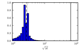
Since marginalizing the coherent SNR results in the creation of a single virtual detector, this motivates the construction of an average mass metric using this virtual detector’s harmonic sum PSD. In Fig. 1, we compare this virtual detector’s mass metric to a numerically-marginalized metric (i.e., the metric of (IV.2)) projected down to the mass subspace. We find excellent agreement between these two metrics.

Figure 1: We show 3% mismatch ellipses associated with different mass metrics for a single point in the mass parameter space. The many transparent ellipses come from different choices of the sky location, polarization, and inclination angle, each chosen randomly with the appropriate distribution. The dashed ellipse shows the metric numerically-marginalized using a $P(\mathcal{D})=\mathcal{D}^{2}$ distribution, and projected down to the mass subspace. The dotted ellipse shows the single-detector mass metric obtained by using the harmonic sum PSD.

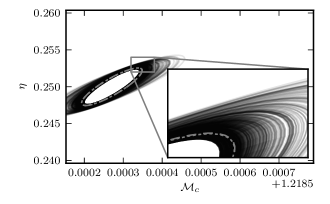
It is interesting to note that the coherent SNR is numerically equal to the sum of squares of the SNRs that are obtained from the detectors individually Harry and Fairhurst (2011), which is how the network SNR is computed for coincident searches. Because of this, we propose that when a single template bank is desired for use in coincident searches, either the mass metric (or inner products) used in the template placement algorithm be computed with the harmonic sum PSD.

It should be noted that when one is constructing a mass metric for a single set of sky parameters, this introduces Dirac delta-functions, $\delta(\alpha-\alpha_{0})$ and $\delta(\delta-\delta_{0})$, into the marginalization integrals of the detector responses. This leads us to use a weighted harmonic sum PSD for the virtual detector’s PSD, where the weighting for detector $Y$ is $\left(F^{Y}_{+}(\alpha_{0},\delta_{0})\right)^{2}+\left(F^{Y}_{\times}(\alpha_{0},\delta_{0})\right)^{2}$.

V.2 Sky metric

Just as we would like to create a sky-location-independent metric for the mass subspace, we would like to create a mass-parameter-independent metric for the sky-location subspace. From Fairhurst (2009); Wen and Chen (2010); Fairhurst (2011, 2012), it has been found that the sky localization accuracy associated with a network of GW detectors is dependent on the signal-weighted bandwidth of the detectors and the physical separation of the detectors.

For short-duration, nonprecessing inspiral signals expanded to Newtonian order in the amplitude, the power of the signal is given by $|h|^{2}\propto f^{-7/3}$, which is independent of the mass of the source objects. The relevant part of the waveform that does depend on the mass of the source objects is the upper frequency cutoff associated with the termination of the waveform, which is inversely proportional to the total mass of the binary. This implies that the signals with the lowest total masses will have the largest signal-weighted bandwidth, and thus the best sky-localization accuracy. Because of this, we propose to construct a single sky-space template bank for the particular mass space given by the computing the marginalized metric from the lowest total mass binary.

Figure 2: We show the metric density as a function of the sky parameters for the marginalized metric where the mass subspace has been projected out. This metric was computed for the HLV network of advanced GW detectors.

Figure 3: We show the metric density as a function of the sky parameters for the extrema-averaged metric where the mass subspace has been projected out. This metric was computed for the HLV network of advanced GW detectors.

Figure 4: We show $D$, (6), for the HLV network of GW detectors. The patterns of small $D$ seen here overlap with the patterns of large metric density in Fig. 3. This is due to the fact that $D$ is in the denominator of the extrema-averaged metric.

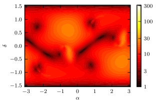
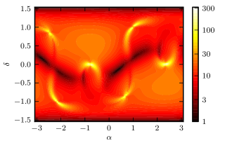
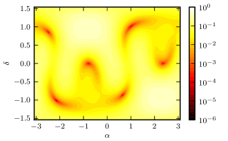
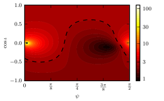
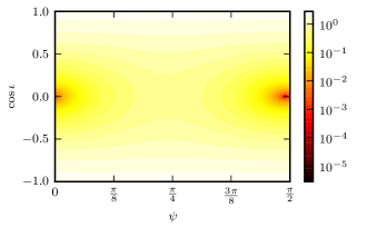
In Fig. 2 we show the variation of the marginalized sky metric density associated with the HLV network of detectors as a function of the source sky position, assuming the aLIGO The LIGO Scientific Collaboration (2009) and Adv. Virgo The Virgo Scientific Collaboration (2010) PSDs and a signal from a BNS system with $m_{1}=m_{2}=1.4M_{\odot}$. This should be compared with Fig. 3, which shows the extrema-averaged sky metric density. We see that there is more variation (and higher metric densities) associated with this metric than with the marginalized metric. To understand this, let us look at the form of (12), and in particular concentrate on the term in the denominator, recalling that $D$ is given by (6). Figure 4 shows how $D$ varies as a function of sky location. We see that points for which $D$ becomes near singular exhibit the largest metric densities of Fig. 3.

A qualitative understanding of why this occurs can be obtained by studying the network response in a different coordinate system. In particular, if we introduce an additional polarization angle between the geocentric frame and the radiation frame, we find that choosing a particular value for this angle can maximize the network response to one polarization, typically chosen to be the new plus polarization. This is called the transformation to the dominant polarization frame Klimenko et al. (2005, 2006); Sutton et al. (2010); Harry and Fairhurst (2011); Bose et al. (2011). In particular, the detector polarization responses for detector $Y$ are transformed as

$$F_{+}^{\mathrm{DP},Y}=F_{+}^{Y}\cos 2\chi^{\mathrm{DP}}+F_{\times}^{Y}\sin 2\chi^{\mathrm{DP}},$$ (28)

$$F_{\times}^{\mathrm{DP},Y}=-F_{+}^{Y}\sin 2\chi^{\mathrm{DP}}+F_{\times}^{Y}\cos 2\chi^{\mathrm{DP}},$$ (29)

where

$$\tan 4\chi^{\mathrm{DP}}=\frac{2C}{A-B}.$$ (30)

This choice of angle causes $C^{\mathrm{DP}}=0$, which diagonalizes the maximum likelihood ratio matrix $\mathcal{M}$. The network response power of the two different polarizations in this frame is found to be

$$A^{\mathrm{DP}}=\frac{1}{2}\left(A+B+\sqrt{\left(A+B\right)^{2}-4D}\right),$$ (31)

$$B^{\mathrm{DP}}=\frac{1}{2}\left(A+B-\sqrt{\left(A+B\right)^{2}-4D}\right),$$ (32)

which yields a total network response power of $A+B$. When $4D\ll(A+B)^{2}$, these approximate to

$$A^{\mathrm{DP}}\approx A+B-\frac{D}{A+B},$$ (33)

$$B^{\mathrm{DP}}\approx\frac{D}{A+B},$$ (34)

Thus we see that $D/(A+B)$ can be understood to be the network response power of the subdominant polarization. This implies that the extrema-averaged metric is dominated by locations where the network is sensitive to essentially only one polarization.

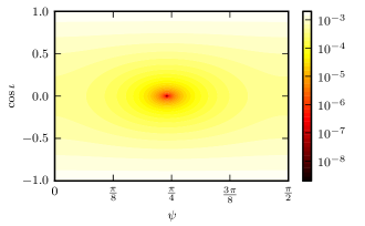
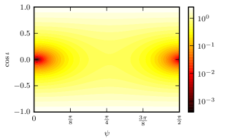
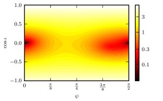
This is further investigated in Fig. 5 where we look at the amplitude parameter dependent metric density for a sky direction where $D$ is almost singular. We find that the amplitude parameter dependent metric density is largest for combinations of amplitude parameters that produce the smallest coherent SNRs associated with the dominant polarization. As expected, the coherent SNR weighting associated with the marginalized metric overwhelms these regions of large metric density.

Figure 5: 5 shows the amplitude dependent metric density, $\sqrt{|g|}$, associated with the sky parameters for a sky location where $D$ is near singular as a function of $\cos\iota$ and $\psi$. The solid (dashed) contour shows the density of the extrema-averaged (marginalized) metric. 5 shows a normalized histogram of $\sqrt{|g|}$. The vertical solid and dashed lines again show the density of the extrema-averaged metric and marginalized metric, respectively. In addition, the vertical dotted line shows the average value of $\sqrt{|g|}$. 5, 5, and 5 shows the coherent SNR associated with the dominant polarization, subdominant polarization, and their sum, respectively, as a function of $\cos\iota$ and $\psi$. It is observed that the regions where $\sqrt{|g|}$ is large, the coherent SNR associated with the dominant polarization is small. 5 shows that for the density of the $\rho^{2}$-weighted metric (i.e., the integrand of the marginalized metric), the coherent SNR weighting overwhelm the regions of large $\sqrt{|g|}$.

VI Conclusion

We have derived a marginalized metric that can be used for template placement associated with coherent searches for short-duration nonprecessing inspiral GW signals in data from a network of GW detectors. The marginalized metric emphasizes combinations of parameters that are more detectable than previously proposed average metrics. This will help to focus computational resources on regions of the extrinsic parameter space from which GWs are more likely to be detected. In addition, we have shown how the marginalized metric can be effectively separated into two two-dimensional metrics associated with the sky and mass subspaces, respectively.

The marginalized metric is shown to take the same form when performing searches for signals from randomly oriented systems (associated with “all-sky” searches) and signals from (anti-)aligned systems (associated with searches targeting GWs from the progenitors of short GRBs).

The metric for the mass subspace is found to be well approximated by a single-detector metric that is based on the harmonic sum of the PSDs of detectors in the network. This metric is equally valid for coincidence-based searches and coherent searches.

The metric for the sky subspace is found based on using the largest bandwidth signal from the parameter space. The marginalized sky metric is compared to the extrema-averaged sky metric. High density regions of the sky associated with the extrema-averaged sky metric are found to be associated with locations where the network response to the subdominant polarization is nearly singular and the network response to the dominant polarization is small. This involved computing the network response to the dominant and subdominant polarizations in terms of $\mathcal{F}$-statistic quantities. Indeed, for an example sky location, combinations of the inclination angle and polarization angle that contribute to the high density of the extrema-averaged sky metric are shown to have a small contribution to the marginalized sky metric.

These results will be useful in constructing template banks for either coincident or coherent searches for short-duration, nonprecessing inspiral signals in GW data from the second generation GW detectors.

Appendix A Amplitude Parameters

The detector independent amplitude parameters associated with our model for short-duration, nonprecessing inspiral GW signals are given as

$$\mathcal{A}^{1} :=\;\;\;\mathscr{A}_{+}\cos{\phi_{0}}\cos{2\psi}-\mathscr{A}_{\times}\sin{\phi_{0}}\sin{2\psi},$$ (35)

$$\mathcal{A}^{2} :=\;\;\;\mathscr{A}_{+}\cos{\phi_{0}}\sin{2\psi}+\mathscr{A}_{\times}\sin{\phi_{0}}\cos{2\psi},$$

$$\mathcal{A}^{3} :=-\mathscr{A}_{+}\sin{\phi_{0}}\cos{2\psi}-\mathscr{A}_{\times}\cos{\phi_{0}}\sin{2\psi},$$

$$\mathcal{A}^{4} :=-\mathscr{A}_{+}\sin{\phi_{0}}\sin{2\psi}+\mathscr{A}_{\times}\cos{\phi_{0}}\cos{2\psi},$$

where the polarization amplitudes $\mathscr{A}_{+}$ and $\mathscr{A}_{\times}$ are given by

$$\mathscr{A}_{+}:=\frac{h_{0}}{2}(1+\cos^{2}{\iota}),\;\mathscr{A}_{\times}:=h_{0}\cos{\iota}.$$ (36)

Appendix B Basis Waveforms

The four detector-dependent polarization-weighted basis waveforms $\{h_{\mu}^{Y}(t)\}$ are defined to be

$$h_{1}^{Y}(t) :=F_{+}^{Y}(t-t^{Y})h_{c}(t-t^{Y}),$$ (37)

$$h_{2}^{Y}(t) :=F_{\times}^{Y}(t-t^{Y})h_{c}(t-t^{Y}),$$

$$h_{3}^{Y}(t) :=F_{+}^{Y}(t-t^{Y})h_{s}(t-t^{Y}),$$

$$h_{4}^{Y}(t) :=F_{\times}^{Y}(t-t^{Y})h_{s}(t-t^{Y}),$$

where $F_{+}^{Y}$ and $F_{\times}^{Y}$ are the responses of detector $Y$ to the plus and cross polarization waveforms, respectively. For signals that satisfy the long wavelength limit approximation Rakhmanov et al. (2008), these can be defined as the double contraction of two tensors Prix (2012),

$$F_{+}^{Y}(t):=\epsilon_{+}^{ij}d^{Y}_{ij}(t),\;F_{\times}^{Y}(t):=\epsilon_{\times}^{ij}d^{Y}_{ij}(t),$$ (38)

where $d^{Y}_{ij}(t)$ is the detector response tensor and $\{\epsilon_{+,\times}^{ij}\}$ are the polarization-independent basis tensors of the radiation frame. For an interferometric detector, the detector response tensor is given by

$$d^{Y}_{ij}(t)=\frac{1}{2}\left\{\hat{l}^{Y}_{1}(t)\otimes\hat{l}^{Y}_{1}(t)-\hat{l}^{Y}_{2}(t)\otimes\hat{l}^{Y}_{2}(t)\right\}_{ij},$$ (39)

where $\hat{l}^{Y}_{1}$ $(\hat{l}^{Y}_{2})$ is the unit vector pointing along interferometer $Y$’s first (second) arm away from the interferometer’s vertex. As defined in Keppel (2012); Prix (2012), the polarization-independent basis tensors can be built from the basis vectors of the radiation frame $\{\hat{\xi},\hat{\eta},-\hat{n}\}$, where $-\hat{n}$ is the direction of propagation, and $\{\hat{\xi},\hat{\eta}\}$ are basis vectors in the wave-plane (i.e., the plane perpendicular to direction of propagation). The basis vectors $\hat{\xi}$ and $\hat{\eta}$ can be defined with respect to $\hat{n}$ as

$$\hat{\xi}:=\frac{\hat{n}\times\hat{z}}{\left\lvert\hat{n}\times\hat{z}\right\rvert},\;\hat{\eta}:=\hat{\xi}\times\hat{n}.$$ (40)

In a fixed reference frame centered at the geocenter, where

$$\hat{n}=(\cos{\delta}\cos{\alpha},\cos{\delta}\sin{\alpha},\sin{\delta}),$$ (41)

the wave-plane basis vectors are

$$\hat{\xi}=(\sin{\alpha},-\cos{\alpha},0),$$ (42)

$$\hat{\eta}=(-\sin{\delta}\cos{\alpha},-\sin{\delta}\sin{\alpha},\cos{\delta}).$$ (43)

Using these conventions, the polarization-independent basis tensors are given as

$$\epsilon^{ij}_{+} :=\left\{\hat{\xi}\otimes\hat{\xi}-\hat{\eta}\otimes\hat{\eta}\right\}^{ij},$$ (44)

$$\epsilon^{ij}_{\times} :=\left\{\hat{\xi}\otimes\hat{\eta}+\hat{\eta}\otimes\hat{\xi}\right\}^{ij}.$$

Appendix C Amplitude Parameter Integrals

Here we compute integrals of products of the amplitude parameters over the physical parameters that compose them. Since these amplitude parameters are used in conjunction with either $\mathcal{M}_{\mu\nu}$ or $\mathcal{G}_{\mu\nu ij}$ summed over the free indices, and since $\mathcal{M}_{\mu\nu}$ and $\mathcal{G}_{\mu\nu ij}$ have the same symmetries, we make use of those symmetries to compute only the necessary combinations of products of the amplitude parameters. Those combinations are

$$(\mathcal{A}^{1}\mathcal{A}^{1}+\mathcal{A}^{3}\mathcal{A}^{3}) =\mathscr{A}_{+}^{2}\cos^{2}(2\psi)+\mathscr{A}_{\times}^{2}\sin^{2}(2\psi),$$ (45)

$$(\mathcal{A}^{2}\mathcal{A}^{2}+\mathcal{A}^{4}\mathcal{A}^{4}) =\mathscr{A}_{+}^{2}\sin^{2}(2\psi)+\mathscr{A}_{\times}^{2}\cos^{2}(2\psi),$$ (46)

$$(\mathcal{A}^{1}\mathcal{A}^{2}+\mathcal{A}^{3}\mathcal{A}^{4}) =(\mathscr{A}_{+}^{2}-\mathscr{A}_{\times}^{2})\cos(2\psi)\sin(2\psi),$$ (47)

$$(\mathcal{A}^{1}\mathcal{A}^{4}-\mathcal{A}^{2}\mathcal{A}^{3}) =\mathscr{A}_{+}\mathscr{A}_{\times}.$$ (48)

We are interested in integrals of these quantities of the form

$$\int_{0}^{2\pi}\int_{0}^{2\pi}\int_{0}^{\pi}(\cdot)\sin\iota\,\mathrm{d}\phi_{0}\,\mathrm{d}\psi\,\mathrm{d}\iota,$$ (49)

where $(\cdot)$ refer to one of the combinations of amplitude parameters in (45). Performing these integrals for each of the combinations of amplitude parameters above, we find that the only nonzero combinations are

$$\int_{0}^{2\pi}\int_{0}^{2\pi}\int_{0}^{\pi}(\mathcal{A}^{1}\mathcal{A}^{1}+\mathcal{A}^{3}\mathcal{A}^{3})\sin\iota\,\mathrm{d}\phi_{0}\,\mathrm{d}\psi\,\mathrm{d}\iota=\\ \int_{0}^{2\pi}\int_{0}^{2\pi}\int_{0}^{\pi}(\mathcal{A}^{2}\mathcal{A}^{2}+\mathcal{A}^{4}\mathcal{A}^{4})\sin\iota\,\mathrm{d}\phi_{0}\,\mathrm{d}\psi\,\mathrm{d}\iota=\frac{8\pi^{2}h_{0}^{2}}{5}.$$ (50)

If we assume the orbital angular momentum vector is parallel to the line of site, as is the case for when we are searching for signals associated with GRBs, we obtain

$$\int_{0}^{2\pi}\int_{0}^{2\pi}(\mathcal{A}^{1}\mathcal{A}^{1}+\mathcal{A}^{3}\mathcal{A}^{3})|_{\iota=\iota_{0}}\,\mathrm{d}\phi_{0}\,\mathrm{d}\psi =$$

$$\int_{0}^{2\pi}\int_{0}^{2\pi}(\mathcal{A}^{2}\mathcal{A}^{2}+\mathcal{A}^{4}\mathcal{A}^{4})|_{\iota=\iota_{0}}\,\mathrm{d}\phi_{0}\,\mathrm{d}\psi =4\pi^{2}h_{0}^{2},$$ (51)

$$\int_{0}^{2\pi}\int_{0}^{2\pi}(\mathcal{A}^{1}\mathcal{A}^{4}-\mathcal{A}^{2}\mathcal{A}^{3})|_{\iota=\iota_{0}}\,\mathrm{d}\phi_{0}\,\mathrm{d}\psi =\pm 4\pi^{2}h_{0}^{2},$$ (52)

where the $\pm$ in the third term is associated with inclination angles of $\iota_{0}=\{0,\pi\}$. We assume is it equally likely that when we observe a GRB, the orbital angular momentum is pointing towards us or away from us, thus the last term above will average to zero. Since the same average combinations of the amplitude parameters are non-zero as in the unknown inclination angle case and the same average values for the combinations of marginalized parameters will be found in the numerator and denominator of the marginalized metric, the metric used for searching for GW signals associated with GRBs is the same as in the unknown inclination angle case.

References

- Harry (2010) G. M. Harry (LIGO Scientific Collaboration), Class.Quant.Grav. 27, 084006 (2010).
- Willke et al. (2006) B. Willke, P. Ajith, B. Allen, P. Aufmuth, C. Aulbert, et al., Class.Quant.Grav. 23, S207 (2006).
- Grote and the LIGO Scientific Collaboration (2010) H. Grote and the LIGO Scientific Collaboration, Class. Quant. Grav. 27, 084003 (2010).
- Somiya (2012) K. Somiya (KAGRA Collaboration), Class.Quant.Grav. 29, 124007 (2012).
- The Virgo Collaboration (2009) The Virgo Collaboration, Advanced Virgo Baseline Design, Tech. Rep. VIR–027A–09 (2009).
- Abadie et al. (2010) J. Abadie et al. (LIGO Scientific Collaboration, Virgo Collaboration), Class.Quant.Grav. 27, 173001 (2010), arXiv:1003.2480 [astro-ph.HE] .
- Aasi et al. (2013) J. Aasi et al. (LIGO Scientific Collaboration, Virgo Collaboration), (2013), arXiv:1304.0670 [gr-qc] .
- Owen (1996) B. J. Owen, Phys.Rev. D53, 6749 (1996), arXiv:gr-qc/9511032 [gr-qc] .
- Cokelaer (2007) T. Cokelaer, Phys. Rev. D 76, 102004 (2007).
- Prix (2007) R. Prix, Classical and Quantum Gravity 24, S481 (2007).
- Harry et al. (2009) I. W. Harry, B. Allen, and B. S. Sathyaprakash, Phys. Rev. D 80, 104014 (2009).
- Messenger et al. (2009) C. Messenger, R. Prix, and M. A. Papa, Phys. Rev. D 79, 104017 (2009).
- Manca and Vallisneri (2010) G. M. Manca and M. Vallisneri, Phys. Rev. D 81, 024004 (2010).
- Sathyaprakash and Dhurandhar (1991) B. Sathyaprakash and S. Dhurandhar, Phys. Rev. D 44, 3819 (1991).
- Owen and Sathyaprakash (1999) B. J. Owen and B. Sathyaprakash, Phys.Rev. D60, 022002 (1999), arXiv:gr-qc/9808076 [gr-qc] .
- Brown et al. (2012) D. A. Brown, I. Harry, A. Lundgren, and A. H. Nitz, Phys.Rev. D86, 084017 (2012), arXiv:1207.6406 [gr-qc] .
- Keppel et al. (2013) D. Keppel, A. P. Lundgren, B. J. Owen, and H. Zhu, (2013), arXiv:1305.5381 [gr-qc] .
- Pai et al. (2001) A. Pai, S. Dhurandhar, and S. Bose, Phys.Rev. D64, 042004 (2001), arXiv:gr-qc/0009078 [gr-qc] .
- Keppel (2012) D. Keppel, Phys.Rev. D86, 123010 (2012), arXiv:1208.2340 [gr-qc] .
- Brown (2005) D. A. Brown (LIGO Collaboration), Class.Quant.Grav. 22, S1097 (2005), arXiv:gr-qc/0505102 [gr-qc] .
- Babak et al. (2013) S. Babak, R. Biswas, P. Brady, D. Brown, K. Cannon, et al., Phys.Rev. D87, 024033 (2013), arXiv:1208.3491 [gr-qc] .
- Bose et al. (1999) S. Bose, S. V. Dhurandhar, and A. Pai, Pramana 53, 1125 (1999), arXiv:gr-qc/9906064 [gr-qc] .
- Bose et al. (2000) S. Bose, A. Pai, and S. Dhurandhar, International Journal of Modern Physics D 9, 325 (2000), arXiv:gr-qc/0002010 .
- Finn (2001) L. S. Finn, Phys. Rev. D 63, 102001 (2001), arXiv:gr-qc/0010033 .
- Cutler and Schutz (2005) C. Cutler and B. F. Schutz, Phys. Rev. D 72, 063006 (2005), arXiv:gr-qc/0504011 .
- Harry and Fairhurst (2011) I. W. Harry and S. Fairhurst, Phys. Rev. D 83, 084002 (2011), arXiv:1012.4939 [gr-qc] .
- Prix (2007) R. Prix, Phys. Rev. D 75, 023004 (2007), arXiv:gr-qc/0606088 .
- (28) T. Dal Canton and D. Keppel, “Sensitivity of coincident and coherent inspiral searches at fixed computing cost,” In preparation.
- Fairhurst (2009) S. Fairhurst, New J. Phys. 11, 123006 (2009), arXiv:0908.2356 [gr-qc] .
- Wen and Chen (2010) L. Wen and Y. Chen, Phys.Rev. D81, 082001 (2010), arXiv:1003.2504 [astro-ph.CO] .
- Fairhurst (2011) S. Fairhurst, Class. Quant. Grav. 28, 105021 (2011), arXiv:1010.6192 [gr-qc] .
- Fairhurst (2012) S. Fairhurst, (2012), arXiv:1205.6611 [gr-qc] .
- The LIGO Scientific Collaboration (2009) The LIGO Scientific Collaboration, “Advanced LIGO anticipated sensitivity curves,” (2009).
- The Virgo Scientific Collaboration (2010) The Virgo Scientific Collaboration, “Advanced Virgo psd,” (2010).
- Klimenko et al. (2005) S. Klimenko, S. Mohanty, M. Rakhmanov, and G. Mitselmakher, Phys.Rev. D72, 122002 (2005), arXiv:gr-qc/0508068 [gr-qc] .
- Klimenko et al. (2006) S. Klimenko, S. Mohanty, M. Rakhmanov, and G. Mitselmakher, Journal of Physics: Conference Series 32, 12 (2006).
- Sutton et al. (2010) P. J. Sutton, G. Jones, S. Chatterji, P. M. Kalmus, I. Leonor, et al., New J.Phys. 12, 053034 (2010), arXiv:0908.3665 [gr-qc] .
- Bose et al. (2011) S. Bose, T. Dayanga, S. Ghosh, and D. Talukder, Class.Quant.Grav. 28, 134009 (2011), arXiv:1104.2650 [astro-ph.IM] .
- Rakhmanov et al. (2008) M. Rakhmanov, J. D. Romano, and J. T. Whelan, Classical and Quantum Gravity 25, 184017 (2008), arXiv:0808.3805 [gr-qc] .
- Prix (2012) R. Prix, The F-statistic and its implementation in ComputeFStatistic_v2, Tech. Rep. T0900149-v4 (LIGO Scientific Collaboration, 2012).