Granular systems Nonequilibrium gas dynamics Fluctuation phenomena, random processes, noise, and Brownian motion

High Energy Tail of the Velocity Distribution of Driven Inelastic Maxwell Gases

Abstract

A model of homogeneously driven dissipative system, consisting of a collection of $N$ particles that are characterized by only their velocities, is considered. Adopting a discrete time dynamics, at each time step, a pair of velocities is randomly selected. They undergo inelastic collision with probability $p$. With probability $(1-p)$, energy of the system is changed by changing the velocities of both the particles independently according to $v\rightarrow-r_{w}v+\eta$, where $\eta$ is a Gaussian noise drawn independently for each particle as well as at each time steps. For the case $r_{w}=-1$, although the energy of the system seems to saturate (indicating a steady state) after time steps of $O(N)$, it grows linearly with time after time steps of $O(N^{2})$, indicating the absence of a eventual steady state. For $-1<r_{w}\leq 1$, the system reaches a steady state, where the average energy per particle and the correlation of velocities are obtained exactly. In the thermodynamic limit of large $N$, an exact equation is obtained for the moment generating function. In the limit of nearly elastic collisions and weak energy injection, the velocity distribution is shown to be a Gaussian. Otherwise, for $|r_{w}|<1$, the high-energy tail of the velocity distribution is Gaussian, with a different variance, while for $r_{w}=+1$ the velocity distribution has an exponential tail.

As we observe in everyday life, for example when we drop a marble ball on the floor or play billiard, granular matter dissipates energy through inelastic collisions. A box of marbles needs to be shaken continuously in order to observe movement of the constituents in the system. If the supply of energy from the outside is stopped, such systems comes to the rest in a short time. When the input of energy to the system (“heating”) compensates the energy loss due to collisions (with walls as well as with other particles), one expects an inelastic “gas” to reach a nonequilibrium steady-state. It is tempting to define an “effective temperature” by the average kinetic energy per particle. A natural question is whether the steady-state velocity distribution is Maxwell-Boltzmann or something else.

In this letter we consider a much studied model of driven inelastic granular gases, namely the inelastic Maxwell model. We first point out a subtle effect that has been overlooked in earlier studies — that collisions with walls are necessary for attaining a steady state. We obtain an exact evolution equation for the velocity covariance [eq. (5)] which has an explicit solution. We also obtain several other results in the thermodynamic limit, including an exact equation for the moment generating function [eq. (10)], exact recursion relations for all moments [eq. (High Energy Tail of the Velocity Distribution of Driven Inelastic Maxwell Gases)] and determination of the high-energy tails of the velocity distribution [eq. (16)].

The steady state velocity distributions measured in experiments show deviation from the Maxwellian statistics as well as approach to Gaussian distribution, depending on the experimental conditions [1, 2, 3, 4, 5, 6]. Based on the kinetic theory, an analysis by van Noije and Ernst [7] for a uniformly heated inelastic hard sphere gas, predicts a non-Maxwellian tail $P(v)\sim\exp(-A|v|^{\alpha})$ with $\alpha=3/2$, of the velocity distribution. Barrat et al. [8] find $\alpha=3$ in the limit of vanishing inelasticity (see also [9]). On the other hand, the numerical study of a two-dimensional driven inelastic gas [10] shows a wide range of $\alpha$ ($\alpha<2$) depending on the various system parameters, instead of a universal value. A one-dimensional model of granular system consisting of Brownian particles subject to inelastic mutual collisions, shows a crossover from Gaussian to non-Gaussian distribution, as the ratio of the Brownian relaxation time to the mean collision time is increased [11]. A model of a driven dissipative system was studied in [12] where the energy moments could be computed exactly.

Figure 1: (Color Online) (a) Simulation results for the evolution of the energy per particle $\mathrm{e}(n)$ (red circles) and the velocity correlation $\Sigma(n)$ (orange squares) of $N=5000$ particles system driven by adding uncorrelated white noise ($r_{w}=-1$), for $p=1/2$ and $\epsilon=1/4$. Analytical results are shown by (black) solid and (blue) dashed lines respectively. The $pseudo$ steady state value is shown by the (magenta) dotted line. (b) Simulation results for $\mathrm{e}(n)$ (red circles) and $\Sigma(n)$ (orange squares) with $N=1000$, $p=1/2$ and $\epsilon=1/4$, for $\delta=1$ case. (c) Simulation (red circles) as well as analytical (black solid line) results for $\mathrm{e}(n)$ for $N=5000$, with the dynamics given by eq. (2), with $p=1/2$, $\epsilon=1/4$, and $r_{w}=+1$. The steady state value is shown by the (magenta) dotted line. (d) Simulation (red circles) as well as analytical (black solid line) results for $\mathrm{e}(n)$ for $N=5000$, with the dynamics given by eq. (2), with $p=1/2$, $\epsilon=1/4$, and $r_{w}=1/2$. The steady-state value is shown by the (magenta) dotted line.

Kinetic theory approach to homogeneous granular gases involves setting up the Boltzmann equation for the single-particle velocity distribution, under the molecular chaos hypothesis, which replaces the two-particles velocity distribution function by the product of two single-particle probability density functions (PDFs) $P(v_{1},v_{2})=P(v_{1})P(v_{2})$. For hard spheres, the collision rate is proportional to $|v_{1}-v_{2}|^{\delta}$ with $\delta=1$. In the absence of external driving it has been shown that the velocity distribution has an exponential tail $P(v)\sim\exp({-|v|/v_{0}(t)})$ where $v_{0}(t)$ is the time-dependent thermal speed [13]. In the driven case, uniform heating is modeled by adding a diffusive term $D\partial_{v}^{2}P(v)$ to the Boltzmann equation. Ben-Naim and Krapivsky introduced a simpler model, called inelastic Maxwell model [14], where the collision rate is independent of the velocities of the colliding particles, i.e., $\delta=0$. In this model, an exponential tail $P(v)\sim\exp(-A|v|)$ for the velocity distribution has been obtained [15, 16, 17], while in the limit of vanishing inelasticity, the distribution becomes Gaussian [18].

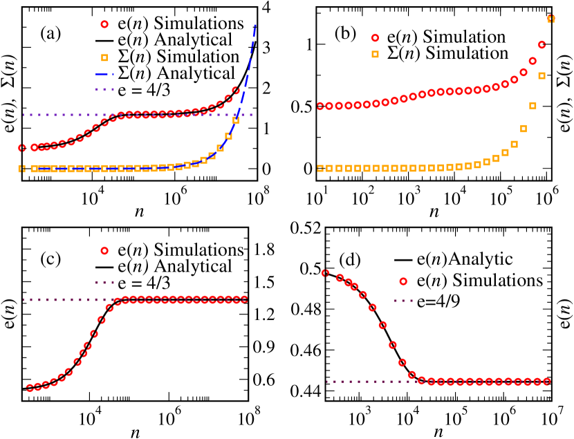
The inelastic Maxwell model is perhaps the simplest model of granular gases. The modeling of velocity change due to an external forcing (heating) by the uncorrelated white noise, $dv_{j}/dt=\eta_{j}(t)$, (which corresponds to the diffusion term in the Boltzmann equation) injects energy, on average, to the system. However, as it turns out, this energy input cannot be balanced by the energy dissipation due to inelastic collisions, and eventually, the average energy of the system increases linearly with time and hence there is no steady state [see fig. 1(a)]. This is true even for $\delta>0$, as seen from fig. 1(b). This is because the inter-particle collision conserves total momentum while the driving noise causes the total momentum to perform a random walk — hence the average energy of the system grows linearly with time. One usually justifies this model of heating by moving to the center of mass velocity frame [19, 14]. However, it is not the experimental situation and hence is unsatisfactory. In fact, as we show below, the external driving is better modeled by a Ornstein-Uhlenbeck process, if one assumes that the external forcing is due to collisions with a wall with a random velocity. While, similar forcing mechanism has been considered earlier for inelastic gases [11, 21, 17, 20], the form of the high-energy tail has not been obtained. In this letter, we obtain several exact results, including the high-energy tail of the velocity distribution.

Here for simplicity, we consider the dynamics in discrete time steps. It is straightforward to obtain the continuum version by taking appropriate limits [22]. Following Ref. [14], ignoring the spatial structure, we consider a collection of $N$ identical particles that are characterized by their velocities $v_{i}$, where $i=1,2,\dotsc,N$. The initial velocities are chosen independently from a Gaussian distribution. At each time step, two particles are chosen at random, and with probability $p$ they undergo inelastic collision and with probability $1-p$ they are subjected to independent external forcing. The two-body inelastic collisions change the velocities of the selected pair from $(v_{i},v_{j})$ to $(v_{i}^{\prime},v_{j}^{\prime})$ according to

$$\begin{split}v^{\prime}_{i}=\epsilon v_{i}+(1-\epsilon)v_{j},\\ v^{\prime}_{j}=(1-\epsilon)v_{i}+\epsilon v_{j}.\end{split}$$ (1)

Here $\epsilon=(1-r)/2$, with $r$ being the coefficient of restitution defined by $(v^{\prime}_{i}-v^{\prime}_{j})=-r(v_{i}-v_{j})$. The elastic collision corresponds to $r=1$. Although $r=0$ corresponds to the completely inelastic case, in this model the particles do not stick to each other and merely possess the same velocity after collision. Therefore, collision conserves both the number of particles and total momentum ($v_{i}^{\prime}+v_{j}^{\prime}=v_{i}+v_{j}$). In fact, as a model of a dissipative system, we can take $\epsilon\in(0,1)$.

$$\begin{split}&X_{n}=\left[\begin{array}[]{>{\displaystyle}c}\mathrm{e}(n)\\ \Sigma(n)\end{array}\right],~{}\qquad C=\left[\begin{array}[]{>{\displaystyle}c}(1-p)\frac{\sigma^{2}}{N}\\ 0\end{array}\right],\quad\text{and}\\[8.53581pt] &R=\left[\begin{array}[]{>{\displaystyle}c>{\displaystyle}c}1-\frac{\left[4p\epsilon(1-\epsilon)+2(1-p)(1-r^{2}_{w})\right]}{N}&\frac{2p\epsilon(1-\epsilon)}{N}{}\\ \hfil\\ \frac{8p\epsilon(1-\epsilon)}{N(N-1)}&1-\frac{\left[4p\epsilon(1-\epsilon)-2(1-p)(1+r_{w})^{2}+4(N-1)(1-p)(1+r_{w})\right]}{N(N-1)}\end{array}\right]\end{split}$$ (6)

$${\rm e} =\frac{(\sigma^{2}/2)\left[2\epsilon(1-\epsilon)+\gamma(1-r_{w}^{2})+2(N-2)\gamma(1+r_{w})\right]}{4\epsilon(1-\epsilon)(1-r_{w}^{2})+\gamma(1-r_{w}^{2})^{2}+(N-2)(1+r_{w})[4\epsilon(1-\epsilon)+2\gamma(1-r_{w}^{2})]}~{},$$ (7)

$$\Sigma =\frac{2\sigma^{2}\epsilon(1-\epsilon)}{4\epsilon(1-\epsilon)(1-r_{w}^{2})+\gamma(1-r_{w}^{2})^{2}+(N-2)(1+r_{w})[4\epsilon(1-\epsilon)+2\gamma(1-r_{w}^{2})]}~{}.$$ (8)

As in Ref. [14], we first apply the external forcing by adding uncorrelated white noises to the velocities ($v^{\prime}=v+\eta$) of the selected pair independently. In this case, starting from an initial state of uncorrelated velocities, we find that [22] for large $N$, after time steps of $O(N)$ the system reaches a steady-state-like state where the average energy per particle saturates to a fixed value [fig. 1(a)]. Although, correlation between velocities builds up over time through collisions, it is $O(1/N)$ in this pseudo steady state and therefore remains negligible. Consequently, the molecular chaos hypothesis, $P(v_{i},v_{j})=P(v_{i})P(v_{j})$, is justified in the pseudo steady state. However, eventually after time steps of $O(N^{2})$, the correlation between velocities no longer remains negligible — both the correlation and the average energy per particle grow linearly with time [fig. 1(a)]. Therefore, the system no longer has a true steady state.

If one assumes that the external forcing is due to collision of a particle with a vibrating wall, then the post-collision velocity $v^{\prime}$ of a particle is related to its pre-collision velocity $v$ and the velocity of the wall $V_{w}$ as $v^{\prime}=-r_{w}v+(1+r_{w})V_{w},$ where $r_{w}$ is the coefficient of restitution for the particle-wall collision and the velocity of the wall is assumed to be unchanged in the collision. Since, the velocity of the wall is random, we denote the term $(1+r_{w})V_{w}$ by a random variable $\eta$ to get $v^{\prime}=-r_{w}v+\eta.$ In an appropriate limit this becomes equivalent to an Ornstein-Uhlenbeck process in continuous time. We will see that this leads to a steady state for $-1<r_{w}\leq 1$.

The dynamics $(v_{i},v_{j})\rightarrow(v^{\prime}_{i},v^{\prime}_{i})$ at each time step, for the pair selected at random, is given by

$$\begin{split}v^{\prime}_{i}&=\chi\bigl{[}\epsilon v_{i}+(1-\epsilon)v_{j}\bigr{]}+(1-\chi)\bigl{[}-r_{w}v_{i}+\eta_{i}\bigr{]},\\ v^{\prime}_{j}&=\chi\bigl{[}\epsilon v_{j}+(1-\epsilon)v_{i}\bigr{]}+(1-\chi)\bigl{[}-r_{w}v_{j}+\eta_{j}\bigr{]},\end{split}$$ (2)

where $\chi$ is a random number which takes values either $1$ or $0$ with probability $p$ and $1-p$ respectively, independently at each step. The noises $\{\eta\}$ at different time steps are drawn independently from a Gaussian distribution with zero mean and variance $\langle\eta_{i}\eta_{j}\rangle=\sigma^{2}\delta_{ij}$.

Let $v_{i}(n)$ be the velocity of the $i-{\rm th}$ particle at the $n-{\rm th}$ time step. The average energy per particle of the system and the velocity correlation between any two particles, at the $n-{\rm th}$ time step are defined as

$${\rm e}(n) =\frac{1}{2N}\;\sum^{N}_{i=1}\;\langle v^{2}_{i}(n)\rangle~{},$$ (3)

$$\text{and}~{}~{}\Sigma(n) =\frac{1}{N(N-1)}\;\sum_{i\neq j}\;\langle v_{i}(n)v_{j}(n)\rangle~{},$$ (4)

respectively. It turns out that they satisfy the following exact recursion relation:

$$X_{n}=RX_{n-1}+C,$$ (5)

where $X_{n}$, $R$, and $C$ are given by

$$see~{}eq.(\ref{wide1})~{}above$$

Equation (5) has the exact solution $X_{n}=R^{n}X_{0}+\sum^{n-1}_{l=0}\;R^{l}C$, with the initial conditions $X_{0}=[\mathrm{e}_{0},0]^{T}$. The two eigenvalues of $R$ can be evaluated explicitly. For $r_{w}=-1$, the eigenvalues are $1$ and $1-p(1-r^{2})/(N-1)$. The unit eigenvalue leads to an eventual linear increase of $X_{n}$. For $r_{w}\neq-1$, both eigenvalues have absolute values less than unity, and hence in the $n\rightarrow\infty$ limit, $X_{n}\rightarrow X_{\infty}$, independent of $n$, as seen in fig. 1(c) and fig. 1(d). Thus, the system reaches a steady state. The energy and correlations in the steady state are given exactly by

$$see~{}~{}eqs.~{}\eqref{wide2a}~{}and~{}\eqref{wide2b}~{}above$$

respectively, where $\gamma=(1-p)/p$, is the ratio of the injection to the collision rate. In the large $N$ limit we get

$$\mathrm{e}=\frac{\gamma\sigma^{2}}{4\epsilon(1-\epsilon)+2\gamma(1-r_{w}^{2})}+O(N^{-1})$$ (9)

and $\Sigma=O(N^{-1})$. Therefore, in the steady state, in the thermodynamic limit $N\to\infty$, the correlations between the velocities vanish. In this limit, it is easy to show that, the moment generating function $Z(\lambda)=\langle\exp(-\lambda v)\rangle$ of the steady-state velocities satisfies the equation

$$Z(\lambda)=pZ(\epsilon\lambda)Z([1-\epsilon]\lambda)+(1-p)Z(r_{w}\lambda)f(\lambda),$$ (10)

where $f(\lambda)=\exp(\lambda^{2}\sigma^{2}/2)$ and we have used the fact that $Z(-\lambda)=Z(\lambda)$ for even distribution. Note that $Z(\lambda)=1+\mathrm{e}\lambda^{2}+\dotsb$ as $\lambda\rightarrow 0$.

In the near-elastic and weak energy injection limit: $\epsilon\rightarrow 0$, $r_{w}=(1-\theta)\rightarrow 1$, $\sigma\rightarrow 0$, while keeping $\sigma^{2}/\epsilon$ and $\theta/\epsilon$ fixed, using the Taylor expansion in eq. (10) we get

$$\frac{dZ}{d\lambda}=\lambda\Delta^{2}Z(\lambda),~{}~{}\text{where}~{}\Delta^{2}=\frac{\gamma\sigma^{2}/\epsilon}{2\bigl{[}1+\gamma\theta/\epsilon\bigr{]}}.$$ (11)

Note from eq. (9) that $\langle v^{2}\rangle\rightarrow\Delta^{2}$ in this limit. Evidently, the solution of eq. (11) is $Z(\lambda)=\exp(\lambda^{2}\Delta^{2}/2)$, which implies the Gaussian velocity distribution

$$P(v)=\frac{1}{\sqrt{2\pi\Delta^{2}}}\exp\left(-\frac{v^{2}}{2\Delta^{2}}\right).$$ (12)

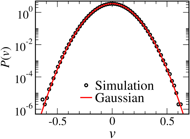
Figure 2 shows a comparison of this result with numerical simulation.

Figure 2: Simulation (black circles) and analytical (red solid line) results for steady state velocity distribution in the near-elastic and weak energy injection limit for $N=100$ with $p=0.5$, $\epsilon=0.005$, $r_{w}=0.99$, and $\sigma=0.02$.

In general, we are not able to find the exact solution of eq. (10). For the case $r_{w}=+1$, we have

$$Z(\lambda)=\bigl{[}1-(1-p)~{}f(\lambda)\bigr{]}^{-1}\,p\,Z(\epsilon\lambda)Z([1-\epsilon]\lambda)~{},$$ (13)

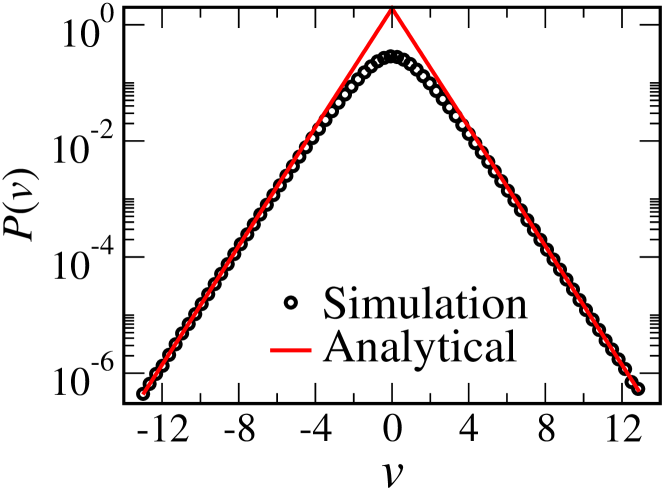
which can be solved by iteration [22]. The tail of the velocity distribution is determined by the pole closest to the origin $\lambda_{0}=\pm\sqrt{-2\ln(1-p)}/\sigma$, which comes from the factor $[1-(1-p)~{}f(\lambda)]^{-1}$ in eq. (13). This gives rise to exponential tails $P(v)\sim A(\epsilon)\exp(-|\lambda_{0}||v|)$, where the prefactor $A(\epsilon)$ is known explicitly. A comparison with the numerical simulation gives very good agreement as shown in fig. 3. We note that eq. (10) is symmetric for $r_{w}\leftrightarrow-r_{w}$. However this equation has been derived under the assumption of a steady state. Therefore for the case $r_{w}=-1$, it is valid only in the pseudo-steady state in which case one indeed finds an exponential tail [14, 15, 16, 17].

Figure 3: Simulation (black circles) and analytical (red solid line) results for steady state velocity distribution for $r_{w}=+1$. The other parameters are $N=100$, $p=0.5$, $\epsilon=1/4$, and $\sigma=1$.

For $|r_{w}|<1$ it is difficult to obtain the tails accurately from direct numerical simulations, as it would require large number of realizations. Equation (10) can be numerically solved and then inverted numerically to obtain $P(v)$. It is convenient to use the characteristic function $Z_{c}(k)=Z(ik)$. For the special case $\epsilon=1/2$ and $r_{w}=1/2$, eq. (10) has a simpler form

$$Z_{c}(k)=pZ_{c}^{2}(k/2)+(1-p)Z_{c}(k/2)\exp(-k^{2}\sigma^{2}/2).$$ (14)

This is useful, as to compute $Z_{c}$ for any $k$ one only requires its value at $k/2$. This “linear structure”, as opposed to the “tree” in the general case, is useful to efficiently compute $Z_{c}(k)$ numerically while using the initial condition $Z_{c}(k)=1-\mathrm{e}k^{2}$ for $k\ll 1$. Finally, numerically computing the inverse Fourier transform of $Z_{c}(k)$ gives the velocity distribution. This is compared with simulation results in fig. 4(c). From the numerical evaluation, we observe the tail $P(v)\sim\exp(-A\mid v\mid^{\alpha})$, with $\alpha$ gradually increasing (but $<2$) as we go towards higher and higher the velocities.

Figure 4: (Colors Online) (a) $\mu(\lambda)$ for $\epsilon=1/2$, and $r_{w}=1/2$ for three different $p$. These curves asymptotically approach the function $(2/3)\lambda^{2}$, shown by the (green) dashed line. (b) The first and second derivatives of $\mu(\lambda)$ and their asymptotic values (green solid line and cyan dashed line respectively). The same symbols and colors are used for the same $p$ values for both $\mu^{\prime}(\lambda)$ and $\mu^{\prime\prime}(\lambda)$. (c) The velocity distribution for the dynamics eq. (2) for $p=1/2$, $\epsilon=1/2$ and $r_{w}=1/2$ from simulation (black “+”) compared with results calculated from the exact inverse Fourier transform of $Z_{c}(k)$ (red solid line) as well as from the saddle point approximation (green dashed line), given by eq. (17).

For $\alpha>1$, the function $Z(\lambda)$ is analytic. If $Z(\lambda)$ is known, then the large deviation tail of the velocity distribution can be obtained by the saddle point approximation

$$P(v)\approx\frac{\exp\bigl{[}\mu(\lambda^{*})+\lambda^{*}v\bigr{]}}{\sqrt{2\pi|\mu^{\prime\prime}(\lambda^{*})|}}~{},$$ (15)

where $\mu(\lambda)=\ln Z(\lambda)$ and the saddle point $\lambda^{*}(v)$ is implicitly given by the equation $\mu^{\prime}(\lambda^{*})=-v$. A careful saddle-point analysis [22] shows that the first term on the right hand side of eq. (10) becomes negligible compared to the left hand side, for $\lambda$ near $\lambda^{*}(v)$ for large $v$. The remaining terms in eq. (10) gives the Gaussian distribution

$$P(v)\approx\sqrt{\frac{1-r_{w}^{2}}{2\pi\sigma^{2}}}\,\exp\left[-\frac{v^{2}}{2\sigma^{2}}(1-r_{w}^{2})\right].$$ (16)

Therefore, the high-energy tail is governed, not by the inelastic collisions amongst the particles, but by the collisions of the particles with the “wall”.

To verify the above result, we numerically compute $Z(\lambda)$ from eq. (10) for $\epsilon=1/2$, $r_{w}=1/2$, and $\sigma=1$, for which $b=2/3$. It is clear from fig. 4(a) that $\mu(\lambda)\sim b\lambda^{2}$ for large $\lambda$. From $\mu(\lambda)$, we also numerically compute $\mu^{\prime}(\lambda)$ and $\mu^{\prime\prime}(\lambda)$ [fig. 4(b)]. Now, each value of $\lambda$ corresponds to a velocity $v=-\mu^{\prime}(\lambda)$, whose PDF, under the saddle point approximation, is numerically obtained using

$$P(v=-\mu^{\prime}(\lambda))\approx\frac{1}{\sqrt{2\pi\mu^{\prime\prime}(\lambda)}}\exp\bigl{[}\mu(\lambda)-\lambda\mu^{\prime}(\lambda)\bigr{]}.$$ (17)

Figure 4(c) compares this with the simulation result as well as with the distribution obtained from the exact numerical inverse Fourier transform of $Z_{c}(k)$.

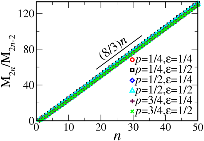
Computing the moments assuming eq. (16) for all $v$, one gets $\langle v^{2n}\rangle=(\sigma^{2}/2)^{n}(1-r_{w}^{2})^{-n}(2n)!/n!$. Certainly this results cannot be valid for small $n$ , e.g., compare the $n=1$ case with $2\mathrm{e}$ form eq. (9). However, for large $n$ one expects this result to agree with the exact result. To compare with the exact result, it is useful to look at the ratio between two successive even moments, $\langle v^{2n}\rangle/\langle v^{2n-2}\rangle\sim 2\sigma^{2}(1-r_{w}^{2})^{-1}n$ for large $n$. We find that the even moments $M_{2n}=\langle v^{2n}\rangle$ satisfies the exact recursion relation

$$\Bigl{[}1-\epsilon^{2n}-(1-\epsilon)^{2n}+\gamma\bigl{(}1-r_{w}^{2n}\bigr{)}\Bigr{]}\,M_{2n}=$$

$$\sum_{m=1}^{n-1}\binom{2n}{2m}\epsilon^{2m}(1-\epsilon)^{2n-2m}M_{2m}M_{2n-2m}$$

$$+\gamma\sum_{m=0}^{n-1}\binom{2n}{2m}r_{w}^{2m}M_{2m}\frac{(2n-2m)!}{(n-m)!}\left(\frac{\sigma^{2}}{2}\right)^{n-m},$$ (18)

with $M_{0}=1$. Using this we compute the moments recursively. Figure 5 confirms that $M_{2n}/M_{2n-2}\rightarrow 2\sigma^{2}(1-r_{w}^{2})^{-1}n$ for large $n$.

Figure 5: The ratios of successive even moments $M_{2n}/M_{2n-2}$ calculated from eq. (High Energy Tail of the Velocity Distribution of Driven Inelastic Maxwell Gases) for $r_{w}=1/2$ and $\sigma=1$.

Interestingly, eq. (10) has an exact solution, when the external noise is drawn from the Cauchy distribution, i.e., $f(ik)=\exp(-a|k|)$. In this case, it can be proved that $Z_{c}(k)=Z(ik)=\exp(-b|k|)$ with $b=a/(1-r_{w})$, which implies the Cauchy law

$$P(v)=\frac{1}{\pi b[1+(v/b)^{2}]}.$$ (19)

Note that this result is independent of the rate parameter $\gamma$ and the coefficient of restitution of the inter-particle collisions. It only depends on the coefficient of restitution $r_{w}$ for the wall-particle collision and the noise parameter $a$.

In conclusion, in this letter we have shown that it is possible to write exact recursion relation for the time evolution of the second moment and velocity correlation together for the driven inelastic Maxwell model. This enables us to obtain the form of the high-energy tails and all moments (recursively) of the velocity distribution in the steady state in the thermodynamic limit. We emphasize that we do not require any approximations to break the BBGKY hierarchy, as has been assumed in earlier work [20] but is unnecessary — the equations close once we also consider correlations [22]. Our results are also valid in the continuum time dynamics.