Investigating the effect of precession on searches for neutron-star–black-hole binaries with Advanced LIGO
Abstract
The first direct detection of neutron-star–black-hole binaries will likely be made with gravitational-wave observatories. Advanced LIGO and Advanced Virgo will be able to observe neutron-star–black-hole mergers at a maximum distance of 900 Mpc. To achieve this sensitivity, gravitational-wave searches will rely on using a bank of filter waveforms that accurately model the expected gravitational-wave signal. The emitted signal will depend on the masses of the black hole and the neutron star and also the angular momentum of both components. The angular momentum of the black hole is expected to be comparable to the orbital angular momentum when the system is emitting gravitational waves in Advanced LIGO’s and Advanced Virgo’s sensitive band. This angular momentum will affect the dynamics of the inspiralling system and alter the phase evolution of the emitted gravitational-wave signal. In addition, if the black hole’s angular momentum is not aligned with the orbital angular momentum it will cause the orbital plane of the system to precess. In this work we demonstrate that if the effect of the black hole’s angular momentum is neglected in the waveform models used in gravitational-wave searches, the detection rate of neutron-star–black-hole systems with isotropic spin distributions would be reduced by in comparison to a hypothetical perfect search at a fixed signal-to-noise ratio threshold. The error in this measurement is due to uncertainty in the post-Newtonian approximations that are used to model the gravitational-wave signal of neutron-star–black-hole inspiralling binaries. We describe a new method for creating a bank of filter waveforms where the black hole has nonzero angular momentum that is aligned with the orbital angular momentum. With this bank we find that the detection rate of neutron-star–black-hole systems would be reduced by . Systems that will not be detected are ones where the precession of the orbital plane causes the gravitational-wave signal to match poorly with nonprecessing filter waveforms. We identify the regions of parameter space where such systems occur and suggest methods for searching for highly precessing neutron-star–black-hole binaries.
I Introduction
The Advanced Laser Interferometer Gravitational Wave Observatory (aLIGO) will begin observing the gravitational-wave sky in 2015 Aasi et al. (2013). When aLIGO reaches design sensitivity, it will be sensitive to a volume of the universe 1000 times greater than the first-generation LIGO detectors Harry et al. (2010). The French-Italian Advanced Virgo (AdV) detector will begin observations shortly after aLIGO, forming a worldwide network of gravitational-wave observatories Aasi et al. (2013); Acernese et al. (2009, ). One of the most interesting sources for aLIGO and AdV is the inspiral and merger of neutron-star–black-hole (NSBH) binaries. It has been argued that Cyg X-3 is a possible NSBH progenitor Belczynski et al. (2013); however, NSBH binaries have not been observed by radio or other electromagnetic observations. The first direct detection of a NSBH binary will likely be made with aLIGO and AdV. Population-synthesis models of binary evolution predict that aLIGO should see 0.2–300 NSBH binaries per year Abadie et al. (2010a). Direct detection of the gravitational waves from NSBH binaries would confirm their existence and allow us to explore the astrophysics behind the formation and evolution of these systems.
The gravitational waves radiated by NSBH binaries are expected to be significantly affected by the black hole’s angular momentum (spin), which is expected to be comparable to the orbital angular momentum of the binary Cutler et al. (1993); Apostolatos et al. (1994); Kidder et al. (1993); Kidder (1995). Spin-orbit coupling changes the gravitational waveform of the binary’s inspiral and merger and can cause the orbital plane of the binary to precess Apostolatos et al. (1994). Coupling between the black-hole spin and the neutron-star spin Kidder (1995), the quadrupole-monopole interaction due to the spheroidal deformation of spinning black holes and neutron stars Poisson (1998) and the “self-spin” interaction Mikoczi et al. (2005) will also affect the gravitational waveform emitted during a NSBH binary inspiral. The resulting changes in the waveform observed by aLIGO carry a great deal of information about the dynamics of the binary. However, optimal searches of aLIGO data must incorporate this dynamics into their waveform models to avoid a reduction in sensitivity and hence the rate of detected events. Variation between the available waveform models, and with nature’s waveforms, will also cause a reduction in sensitivity, we investigate this issue in a companion work Nitz et al. (2013).
Gravitational-wave searches for the merger of two compact objects rely on matched filtering against compact binary merger gravitational waveform models Wainstein and Zubakov (1962, 1968); Allen et al. (2012). Compact binary mergers in quasicircular orbit are described by 15 parameters: the masses, spin magnitude, spin orientations, source orientation, sky location, distance and time and phase of coalescence Peters and Mathews (1963); Thorne (1987). Matched-filter searches must be capable of detecting binary mergers regardless of the parameters of the system. For nonprecessing systems and restricting to the dominant gravitational-wave mode, the extrinsic parameters–source orientation, sky location, distance and coalescence phase–only affect the overall phase and amplitude of the observed gravitational-wave system. Therefore, it is possible to analytically maximize over these extrinsic parameters Allen et al. (2012).
Changing the masses and spin magnitudes of a nonprecessing system will change the intrinsic phase evolution of the system. To be able to detect NSBH systems within the desired parameter range a set of waveforms or “template bank” must be constructed Sathyaprakash and Dhurandhar (1991); Poisson and Will (1995); Owen (1996); Owen and Sathyaprakash (1999); Babak et al. (2006); Balasubramanian et al. (1996); Cokelaer (2007). These waveforms should span the desired range of mass and spins. The standard practice is to construct a bank of waveforms such that any waveform within the parameter space of interest would be recovered with at least 97% of the optimal signal-to-noise ratio (SNR) by at least one waveform in the template bank Babak et al. (2006, 2013) . However, the geometrical placement algorithms employed in the most recent searches for compact binary coalescences in LIGO and Virgo data are only applicable for compact binary systems whose components have no angular momentum–non-spinning systems Abbott et al. (2009a, b); Abadie et al. (2010b, 2012). Stochastic placement algorithms Babak (2008); Harry et al. (2009); Manca and Vallisneri (2010); Ajith et al. (2012) are capable of placing banks of waveforms where the spin of the black hole is aligned with the orbital angular momentum (aligned-spin NSBH) Ajith et al. (2012). However, these algorithms are known to need more templates to cover a parameter space when compared to geometric algorithms Harry et al. (2009). In Brown et al. (2012a) we developed a new geometrical placement algorithm that could place template banks of aligned-spin binary neutron star (BNS) signals. In this work we expand that method to be able to place template banks of aligned-spin NSBH signals.
When precessing systems are considered as template waveforms, the matched-filter search becomes more complex. In this case the extrinsic parameters no longer enter as overall phase and amplitude shifts in the waveform Apostolatos et al. (1994). Previous work has been conducted to explore the affect of precession on gravitational-wave searches and to develop methods to detect precessing systems Apostolatos (1996); Buonanno et al. (2003); Grandclement et al. (2003); Grandclement and Kalogera (2003); Grandclement et al. (2004); Pan et al. (2004); Buonanno et al. (2004, 2005); Abbott et al. (2008); Van Den Broeck et al. (2009); Fazi (2009); Harry and Fairhurst (2011); Ajith et al. (2012); Brown et al. (2012b); Lundgren and O’Shaughnessy (2013). However, these searches, when applied to initial LIGO and Virgo data, have not shown an increase in efficiency with respect to nonprecessing searches Van Den Broeck et al. (2009). This is because the filtering codes allow for increased, and unphysical, freedom when maximizing over extrinsic parameters and because no suitable method to distinguish gravitational-wave signals from non-Gaussian instrumental noise has been developed for these searches. Therefore, searches for NSBH binaries in data from LIGO and Virgo’s most recent science runs ignored spin effects and used quasicircular templates to search for NSBH binaries Abbott et al. (2009a, b); Abadie et al. (2010b, 2012).
The majority of previous work considered the initial LIGO detectors. aLIGO will have a substantially different noise curve than initial LIGO Aasi et al. (2013). Conclusions drawn using the initial LIGO sensitivity curve may not hold when considering aLIGO. A previous study considering aLIGO sensitivity curves has suggested that it may be possible to detect generic, precessing NSBH binaries using aligned-spin waveforms Ajith et al. (2012). However, other studies have suggested that precession may significantly change the gravitational waveform seen by aLIGO, requiring templates that explicitly capture this effect Brown et al. (2012b).
In this paper, we first investigate the effect of ignoring spin on optimal (matched-filter) searches for NSBH binaries with aLIGO. We demonstrate that the quasicircular templates used in initial LIGO will reduce the detection rate by for NSBH systems with masses uniformly distributed between , an isotropic black-hole spin distribution and spin magnitude uniformly distributed between 0 and 1. Over a wider range of uniformly distributed masses, , we find that the detection rate would be reduced by . In both cases this loss in detection rate is compared against a template bank where every signal is matched exactly by the bank of filters. The loss in event rate is greatest for NSBH binaries with large black-hole spins and large mass ratios. The range quoted in both measurements is due to uncertainty in the waveform models used to simulate NSBH gravitational-wave signals. These values also strongly depend on the signal distributions that we selected. If nature does not provide a uniform distribution of masses and an isotropic distribution of masses then these averaged values will change. To account for this, we explore the ability to recover NSBH signals as a function of their spins and masses in Sec. VIII.
We expand upon the method we introduced in Brown et al. (2012a) and construct a bank of templates for aligned-spin NSBH binaries. We demonstrate that this template bank is effectual for recovering the population of aligned-spin NSBH systems that it is designed to detect. We assess the ability of an aligned-spin template bank to detect a population of generic NSBH binaries where the black-hole spin is not constrained to be parallel to the orbital angular momentum. We find using the aligned-spin bank will reduce the detection rate by compared to using a bank where every signal matches exactly with one of the filter waveforms when searching for NSBH waveforms with masses . When restricting the mass range to we find that the detection rate is reduced by . We find that there are regions of the NSBH signal parameter space where precession effects cause a significant reduction in signal-to-noise ratio. These regions are those where the black hole’s angular momentum is large in comparison to the orbital angular momentum. We suggest possible methods for constructing searches that recover these systems. By considering several NSBH waveform models, we demonstrate that our results are robust against possible errors in the post-Newtonian phasing for NSBH binaries.
There has been a great deal of recent work focused on numerically modeling the merger of a black hole and a neutron star Duez (2010); Shibata and Taniguchi (2011); Pannarale (2012); Lackey et al. (2013); Foucart et al. (2013). However, there is not currently any widely available waveform model that includes both the full evolution of a NSBH coalescence and includes precessional effects over the full parameter space that we consider. Therefore, in this work we have restricted ourselves to considering post-Newtonian, inspiral-only signal waveforms and consider only the case of two point particles. If a full inspiral-merger-ringdown, precessing NSBH waveform model becomes available, it would be informative to compare results with that model against those presented here. However, in this work the black-hole mass is restricted to be less than . It has been demonstrated that inspiral-only template banks recover of the signal power of numerically modeled binary black-hole waveforms Brown et al. (2012c); Smith et al. (2013). It has also been demonstrated that nonspinning NSBH mergers with total mass are indistinguishable from binary black-hole mergers with the same masses Foucart et al. (2013). With these observations we expect that our results are qualitatively valid in the parameter space we study.
The layout of this work is as follows. In Sec. II we describe the set of NSBH systems that we use to assess the performance of our template banks. In Sec. III we discuss the waveform models that we use in our simulations. In Sec. IV we discuss the methods we use to test the template banks. In Sec. V we describe our new method to create banks of aligned-spin filter waveforms and use these methods in Sec. VI to create our template banks. In Sec. VII we validate our template banks against the aligned-spin signal models they are constructed to detect. In Sec. VIII we assess the performance of non-spinning template banks to search for generic NSBH signals and assess the performance of aligned-spin template banks to detect the same signals. We conclude in Sec. IX. Throughout this work we will use .
II A population of NSBH binaries
In this section, we describe our large simulated set of NSBH binaries. This is used to assess the loss in detection rate when using nonspinning and aligned-spin template banks to search for generic NSBH binaries. To construct this set we incorporate current astrophysical knowledge to choose the distribution of masses and spins. However, this astrophysical knowledge is limited due to the fact that no NSBH binaries have been directly observed. Nevertheless, both neutron stars and black holes have been observed in other binary systems, and these observations can be used to make inferences about the mass and spin distributions that might be expected in NSBH binaries. We begin by giving the distributions that we use in this work, before describing the astrophysical knowledge that motivated these choices.
We simulate 100000 NSBH binaries with parameters drawn from the following distribution. The black-hole mass is chosen uniformly between 3 and 15 solar masses; the neutron-star mass is chosen uniformly between 1 and 3 solar masses; the black-hole dimensionless spin magnitude is chosen uniformly between 0 and 1 and the neutron-star dimensionless spin magnitude is chosen uniformly between 0 and 0.05. The initial spin orientation for both bodies, the source orientation and the sky location are all chosen from an isotropic distribution.
Black holes observed in x-ray binaries can be used to estimate the BH mass distribution, though it is difficult to disentangle the individual masses and inclination angle with only electromagnetic observations Ozel et al. (2010). Using a population of low-mass x-ray binary systems with estimated masses, two separate works found that a BH mass distribution of fits the observed data well Ozel et al. (2010); Farr et al. (2011). There is evidence that there is a “mass gap” between and where BHs will not form Ozel et al. (2010); Farr et al. (2011), although this may be due to observational bias Kreidberg et al. (2012). When high-mass x-ray binary systems are considered the mass distribution increases to , although a Gaussian model is a poor fit for these systems Farr et al. (2011). Evidence exists for a stellar mass black hole with mass in the IC 10 X-1 x-ray binary Prestwich et al. (2007); Silverman and Filippenko (2008). We choose to use a uniform range of 3-15 solar masses for the black holes in our NSBH signal population. This is partly motivated by the considerations above, and partly by our concern of the validity of inspiral-only, point particle waveform models for high-mass NSBH systems. Observations of black-hole spin have found spin values that span the minimum and maximum possible values for Kerr black holes Miller et al. (2009); therefore, we use a uniform black-hole spin distribution between 0 and 1.
Observations of NSs in binary systems other than NSBH binaries can be used to estimate the NS mass distribution. Using a population of six BNS systems with well constrained masses, Ozel et al. Ozel et al. (2012) found that the NS mass distribution was well fitted by , in agreement with Kiziltan, Kottas and Thorsett’s result of Kiziltan et al. (2010). However, nonrecycled NSs in eclipsing high-mass binaries, as well as slow pulsars, are found to have a much wider mass distribution of Ozel et al. (2012). Recycled NSs are found to have a higher range of masses, , due to accretion Ozel et al. (2012). However, it is expected that the black hole would form first in the vast majority of cases, which would remove the possibility of recycling. There is also evidence for a NS with a mass as high as Freire et al. (2007), which is very close to the theoretical upper limit on a NS mass of Rhoades and Ruffini (1974). While a conservative choice, we choose to use a uniform mass distribution between 1 and 3 solar masses for the NSs in our NSBH signal population.
The magnitude of the dimensionless spin, , of a neutron star cannot be larger than 0.7 Lo and Lin (2011) as the neutron star would break apart under the rotational force. However, it is rather unlikely that NS spins will have values as large as this in NSBH systems. At birth, neutron star spins are believed to be in the range 10-140 ms, corresponding to Lorimer (2008); Mandel and O’Shaughnessy (2010). Recycled neutron stars can have larger spin values Bildsten et al. (1997); however, they are unlikely to have periods less than 1 ms Chakrabarty (2008), corresponding to a dimensionless spin of . The fastest spinning recycled neutron star observed in a BNS binary has a spin period of only 23 ms Burgay et al. (2003). As astrophysical observations seem to suggest that large neutron spins will be unlikely in NSBH binaries we choose a uniform NS spin distribution between 0 and 0.05.
III Waveform models
Matched-filter searches require an accurate model of compact binary mergers. In a companion work we investigate the agreement of different waveform families in the NSBH region of parameter space and find a considerable disagreement between waveforms produced by different waveform models, which will reduce detection efficiency Nitz et al. (2013).
In this work we wish to investigate the effects of spin, especially spin-induced precession, while understanding and mitigating any bias in our results due to the choice of waveform approximant. We therefore run all our simulations using two waveform approximants: TaylorT2 Damour et al. (2001) and TaylorT4 Buonanno et al. (2003).
Post-Newtonian (PN) waveforms, such as TaylorT2 and TaylorT4, are constructed by solving the PN equations of motion to obtain the binary orbits. It is assumed that the binary evolves adiabatically through a series of quasicircular orbits. This is a reasonable assumption as it is expected that the emission of gravitational radiation will circularize the orbits of isolated binaries Peters (1964). The equations of motion then reduce to series expansions of the center-of-mass energy and the gravitational-wave flux , which are expanded as a power series in the orbital velocity :
| (1) | ||||
| (2) |
The various coefficients (,,,) are reviewed in Arun et al. (2009); Buonanno et al. (2009). For terms involving the orbital contribution, the center-of-mass energy and gravitational-wave flux are known to 3.5PN order [ in the parentheses of (1)] Wiseman (1993); Blanchet et al. (1995a, b, 1996, 2002, 2004). For terms involving the spin of the objects, the expansions of the energy and flux are complete to 2.5PN order [ in the parenthesis of (1)] Kidder et al. (1993); Kidder (1995); Arun et al. (2009). In recent work, terms relating to the coupling between the component spins and the orbit have also been computed to 3.5PN order Blanchet et al. (2012); Bohe et al. (2013). We choose not to use these terms in this work because terms relating to the spin(1)-spin(2), quadrupole-monopole and self-spin contributions are not yet known at 3 PN order, so we restrict the spin-related terms to 2.5 PN where these terms are fully known. We do not expect these terms to change the main conclusions of the work as these additional phase evolution terms will have little effect on the precessional evolution of a system.
The orbital phase, is then obtained via the energy balance equation
| (3) |
and by
| (4) |
Here the gravitational-wave frequency is given by twice the orbital phasing frequency and is related to the orbital velocity by , where denotes the total mass of the binary.
The various approximants are constructed via different ways of obtaining the gravitational-wave phase from the equations above.
III.1 TaylorT2 and TaylorF2
The TaylorT2 approximant is constructed by first calculating
| (5) |
Here is used to indicate that is calculated by first expanding it as a Taylor series. Then orbital terms larger than 3.5PN and spin terms larger than 2.5PN are discarded. This is because terms of this order would also depend on unknown terms in the expansion of the center-of-mass energy and the gravitational-wave phase. As the gravitational-wave phase is therefore obtained according to
| (6) |
which can be integrated analytically. In the same manner can be calculated according to
| (7) |
and can then be numerically inverted to obtain and , which are used to construct the waveform.
When constructing a TaylorT2 waveform, one begins at a fiducial starting frequency, chosen to be smaller than the lowest frequency over which to perform the matched filter. In this work, we use Hz as the starting frequency. The waveform is terminated when the frequency reaches the minimum energy condition (MECO), which is the point where
| (8) |
The TaylorF2 approximant is a frequency-domain equivalent of the TaylorT2 approximant and is constructed using the stationary phase approximation Sathyaprakash and Dhurandhar (1991); Cutler and Flanagan (1994); Droz et al. (1999); Blanchet (2006). The TaylorF2 waveforms can be expressed as an analytic expression of the form
| (9) |
where denotes the Fourier transform of , the time-domain gravitational-wave strain, denotes the chirp mass, the luminosity distance to the source and describes the various orientation angles that only affect the amplitude and overall phase of the observed gravitational waveform Allen et al. (2012). The phase is given by
| (10) |
where is the coalescence time and is a constant phase offset. The terms give the various coefficients of the orbital phase, which are summarized in Arun et al. (2009); Buonanno et al. (2009). TaylorF2 waveforms are usually terminated at the frequency corresponding to the inner-most stable circular orbit (ISCO) of a nonspinning system with the given masses Allen et al. (2012).
III.2 TaylorT4 and TaylorR2F4
In contrast to the TaylorT2 approximant, the TaylorT4 approximant introduced in Buonanno et al. (2003) is formed by calculating
| (11) |
Similar to the TaylorT2 approximant, orbital terms larger than 3.5PN and spin terms larger than 2.5PN are discarded from . This is numerically solved to obtain which can then be used to obtain the gravitational-wave phase. The TaylorT4 approximant uses the same start and termination conditions as the TaylorT2 approximant.
The TaylorR2F4 approximant, introduced in Nitz et al. (2013), is a frequency-domain analytical approximation of the TaylorT4 waveform model. It is constructed in the same manner as TaylorF2; however, it uses
| (12) |
instead of Eq. (5). In this case, while is restricted as described above, is truncated to a higher order in . The additional “partial” terms that are obtained in the resulting PN expansion describe the difference between the TaylorT2 and TaylorT4 models. It has empirically been found that TaylorR2F4 matches best with TaylorT4 when is expanded to 4.5PN order or 6PN order Nitz et al. (2013). We only consider these two expansions of TaylorR2F4 in this work.
IV Method for assessing the performance of NSBH searches
In this section we describe the methods we use to assess the efficiency of template banks and the terminology that we will use in the rest of this work. The “overlap” between two waveforms and is defined as
| (13) |
where denotes the noise-weighted inner product
| (14) |
Here, denotes the one-sided power spectral density of the noise in the interferometer. In this work, we model with the aLIGO zero-detuned, high-power design sensitivity curve Harry et al. (2010) and use a lower frequency cutoff, , of 15 Hz.
As gravitational-wave searches for binary mergers analytically maximize over an overall phase and time shift, we define the “match” between two waveforms to be the overlap maximized over a phase and time shift
| (15) |
One can understand this match as the fraction of the optimal SNR that would be recovered if a template was used to search for a signal .
We define the “fitting factor” between a waveform with unknown parameters and a bank of templates to be the maximum match between and all the waveforms in the template bank Apostolatos (1995):
| (16) |
The mismatch
| (17) |
describes the fraction of SNR that is lost due to the fact that the template in the bank that best matches will not match it exactly due to the discreteness of the bank and due to any disagreement between the waveform families used to model the templates and the signals. In previous searches of LIGO and Virgo data using nonspinning template banks, the banks of signals were constructed so that the fitting factor would be greater than 0.97 for any nonspinning signal within the parameter space Babak et al. (2013). This was chosen as a balance between detection efficiency and computational cost. We also construct our aligned-spinning banks with this criterion.
For the precessing NSBH signals that we consider in this work, the fitting factor will depend on the masses, spin magnitudes, spin orientations, sky locations and orientation of the NSBH system used to produce the waveform . We only sample the fitting factor at discrete points corresponding to the distribution of systems described in Sec. II. When showing results from this set of fitting factors we often do so as a function of only two of the various parameters that the fitting factor depends on. When doing this we split the set of fitting factors into a series of bins corresponding to ranges in both of the parameters we are interested in. For each bin we then calculate an “average fitting factor” within that bin. This is done by taking the mean value of the fitting factor from all points within each bin
| (18) |
where denotes the mean average of . However, this measure can often be misleading. The aLIGO detectors have a direction-dependent and orientation-dependent sensitivity. Systems that are poorly aligned with respect to the detector may not have sufficient SNR to be detected, regardless of the fitting factor. A number of systems for which precessional effects are most prominent are ones in which the precessing orbital plane moves through points where the detector has very little sensitivity Brown et al. (2012b). To account for this we make use of the “effective fitting factor,” first defined in Buonanno et al. (2003) as
| (19) |
Here , which describes the optimal SNR of . For each bin, the cube of the effective fitting factor gives, above an arbitrary SNR threshold, the ratio between the fraction of NSBH signals that would be recovered with the discrete template bank that was used and a theoretical continuous template bank that would recover 100% of signal power for any NSBH waveform. We therefore define the “signal recovery fraction” as .
V A new algorithm for constructing template banks of aligned-spin NSBH waveforms
In Brown et al. (2012a) we proposed a method for generating a geometrically placed bank of aligned-spin systems that can be used to search for BNS systems in the advanced detector era. In this section we adapt the methods presented in that work to the case of NSBH systems and describe how to generate template banks that can recover aligned-spin NSBH waveforms. These banks are applicable for waveforms modeled using either the TaylorT2 approximant or the TaylorT4 approximant.
A bank of templates should be placed such that any putative signal within the parameter space of interest would be recovered with a loss in SNR that is always less than some predefined value, usually taken to be 3% Poisson and Will (1995); Owen (1996); Owen and Sathyaprakash (1999); Babak et al. (2006); Cokelaer (2007); Babak et al. (2013). To determine the maximum spacing between templates that meets this criterion, the parameter space metric is used. This approximates the distance between any two points that are close in the parameter space Owen (1996)
| (20) |
with the metric given by
| (21) |
Here describes the parameters of the signal, in this case the masses and the spins. This is also commonly referred to as the Fisher information matrix.
Obtaining an analytic solution for Eq. (21) is much simpler in the frequency domain and therefore frequency-domain waveform models are commonly used when placing a bank of templates Owen (1996); Owen and Sathyaprakash (1999); Babak et al. (2013). We follow that approach and consider only frequency-domain metrics here. It is important to carefully consider which coordinates to use as parameters when using this metric as an approximation to the parameter space distance. If one were to naively use the masses and spins directly as coordinates it would result in a parameter space metric with a large amount of extrinsic curvature, and Eq. (20) would only be valid for small ranges of . In previous searches for nonspinning systems, the “chirp times” were used Owen and Sathyaprakash (1999), defined as
| (22a) | ||||
| (22b) | ||||
as these are the two combinations of the masses that minimize extrinsic curvature.
When the template waveforms include spin it is difficult to identify a parameterization of the waveform for which the metric is locally flat. Instead, in Brown et al. (2012a) we constructed a metric that uses the various coefficients of the expansion of the orbital phase, given by the various terms in Eq. (10), directly as coordinates. Using these coordinates, the parameter space is globally flat. However, for the TaylorF2 metric including terms up to 3.5PN order, the parameter space is eight-dimensional. The physical subspace forms a four-dimensional manifold within this parameter space.
To deal with the increased dimensionality of the space we perform two coordinate transformations Brown et al. (2012a); Ohme et al. (2013). These two coordinate transformations map points from the coordinates into a Cartesian coordinate system where the principal directions are mapped using coordinates denoted by . Specifically, the first coordinate transformation uses the eigenvectors and eigenvalues of the metric to transform to a Cartesian coordinate system. A principal component analysis is then performed to rotate into the frame given by the principal directions of the manifold describing the physical range of masses and spins we consider within the eight-dimensional parameter space. In this Cartesian coordinate system of principal directions we can assess the effective dimension of the parameter space, i.e., the number of directions in which templates actually need to be placed in order to achieve the desired coverage. For the case of the BNS parameter space with the aLIGO power spectral density we found that many of the directions had an extremely small extent and could be neglected entirely. We found that a two-dimensional lattice could efficiently cover the entire space of aligned-spin BNS waveforms Brown et al. (2012a).
Our geometrical placement method is not specific to the BNS area of the parameter space. However, some modifications to the method were necessary when placing a template bank of NSBH waveforms. Our BNS aligned-spin template bank, as described in Brown et al. (2012a), was given in terms of the positions of the points in the eight-dimensional Euclidean parameter space . These points do not correspond directly to physical masses and spins. For this study we want to use time-domain template families and therefore we must translate the bank into physical parameters. However, if a set of values is given it will, in general, not be possible to find a set of masses and spins that give the exact values. As templates are normally placed in a two-dimensional lattice, we need only to find a physical point that has the corresponding values of and and any value of the other values that correspond to a waveform within the physically allowed manifold. For some cases where a two-dimensional lattice is not sufficient to cover the space we will also specify values of and . We attempt to find a physical solution that is sufficiently close to the desired point using a numerical solution. We generate a large set of points in the mass and spin space and map these points to the parameters. For each template we then find the closest point from our large set of physical points. We then proceed to iteratively test physical points in the vicinity to find a match of at least 0.9999 with the intended position. If the template is within the physically allowed parameter space we can generally find a physical point that has the desired match with the intended point. Templates on the boundaries of the space, might have an overlap as low as with the edge of the physical parameter space. Our method pushes such points back into the desired physical space thereby providing a slight improvement in the bank coverage. This method also provides an easy method to determine the extent of the physical space: if no physical point is found with 0.97 or higher match with the position then that point is not within the physical extent of the parameter space and no template needs to be placed there.
The downside to our brute-force numerical method is that it is currently not computationally efficient; generating a bank with this numerical technique can take hours when running on CPU cores. The cost of placing a bank using this method, however, is negligible when compared to the cost of filtering data against a bank of templates if a single bank is used to filter O(days) of data. If the bank is regenerated every hour, as in previous searches of LIGO and Virgo data Babak et al. (2013), this cost would not be negligible. We note that it should be possible to optimize our implementation to obtain a significant speed increase over what we quote above.
The TaylorF2 metric can be used to place a bank of waveforms modeled with the TaylorT2 approximant. However, we also require that our template placement algorithm place a bank of waveforms that can detect aligned-spin signals modeled using TaylorT4 with no more loss in SNR than that specified by the minimal match of the bank. This will allow us to investigate the efficiency of aligned-spin banks to search for precessing NSBH signals using two waveform models. Using two models will help to mitigate any bias in our results that arises due to the choice of waveform approximant. We investigate the distribution of fitting factors when using a template bank constructed using the TaylorF2 metric to search for aligned-spin TaylorT4 NSBH signals in Sec. VII and find that this would result in a reduction of sensitivity. We therefore make use of a metric that models the TaylorT4 waveform well. To do this we use the TaylorR2F4 waveform model. We have found that restricting the TaylorR2F4 model to terms no larger than 4.5PN and placing a bank of templates using the ensuing metric is sufficient to cover the TaylorT4 parameter space. This is a 12-dimensional metric. We then perform the same rotations as for the TaylorF2 metric to identify the directions for our TaylorR2F4 parameter space and proceed in the same manner as described above.
In contrast to BNS mergers, NSBH systems can merge in the sensitive band of the advanced detectors. Existing nonspinning template placement algorithms Poisson and Will (1995); Owen (1996); Owen and Sathyaprakash (1999); Babak et al. (2006); Cokelaer (2007) as well as our aligned-spin algorithm must use the same termination frequency when modeling waveforms across the parameter space. The standard approach is to assume that the waveforms will follow the TaylorF2, or TaylorR2F4, evolution up to the Nyquist frequency, usually 2048 Hz. For BNS systems, the merger generally occurs above 1000 Hz where the sensitivity of gravitational wave interferometers falls off and therefore little power is incurred between 1000 Hz and Nyquist. Even a BNS has an ISCO with a frequency of 730 Hz. In contrast, a NSBH system has an ISCO frequency at 240 Hz. We must therefore consider what frequency cutoff is most appropriate to use when placing a bank of NSBH waveforms.
We found that using an upper frequency cutoff that is higher than the waveform’s termination frequency results in overcoverage in the parameter space. This result is expected as the subdominant PN terms can have a significant effect in the late part of the evolution, causing systems with the same chirp masses but different spins and mass ratio to diverge faster. Therefore we use an upper frequency cutoff of 1000 Hz for all waveforms within the NSBH parameter space to generate a template bank that will cover to the desired minimal match. However, as this template bank will overcover at least the high-mass end of the parameter space we also investigate the efficiency of banks placed with smaller upper frequency cutoffs in Sec. VII.1. This choice will be an important consideration in the advanced detector era given limits on computational power for conducting NSBH searches.
VI Constructing template banks of aligned-spin NSBH waveforms with our new algorithm
| Template bank | Approximant | Waveform cutoff frequency | Number of templates in bank |
|---|---|---|---|
| Geometric nonspinning bank | TaylorF2 | 1000 Hz | 117,632 |
| Geometric nonspinning bank | TaylorR2F4 (up to 4.5PN) | 1000 Hz | 99,309 |
| Geometric aligned-spin bank | TaylorF2 | 1000 Hz | 817,460 |
| Geometric aligned-spin bank | TaylorF2 | 400 Hz | 432,537 |
| Geometric aligned-spin bank | TaylorF2 | 240 Hz | 282,090 |
| Stochastic aligned-spin bank | TaylorF2 | Dynamic | 971,105 |
| Geometric aligned-spin bank | TaylorR2F4 (up to 4.5PN) | 1000 Hz | 1,100,277 |
| Geometric aligned-spin bank | TaylorR2F4 (up to 4.5PN) | 400 Hz | 504,132 |
| Geometric aligned-spin bank | TaylorR2F4 (up to 4.5PN) | 240 Hz | 260,325 |
| Stochastic aligned-spin bank | TaylorR2F4 (up to 4.5PN) | Dynamic | 1,327,175 |
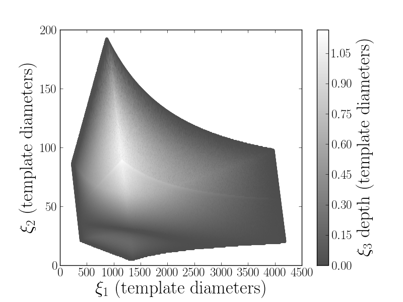
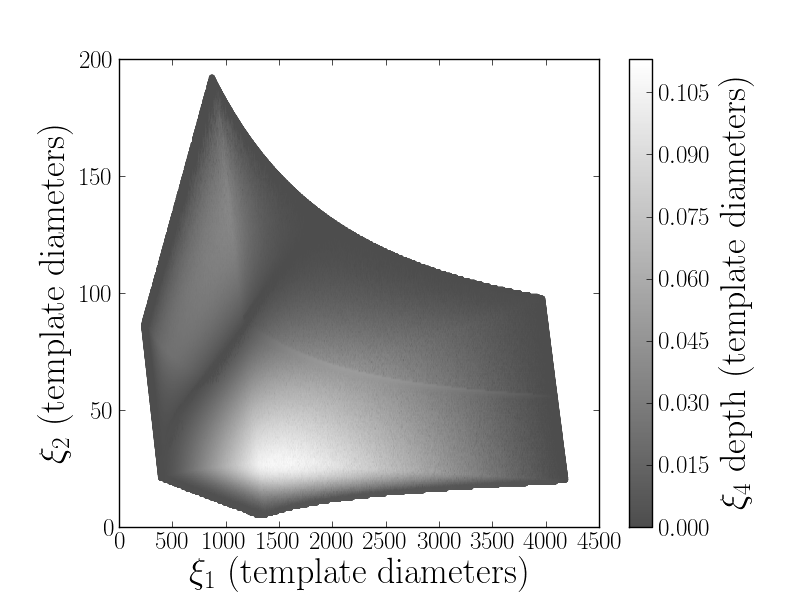
We begin by creating a template bank using the TaylorF2 parameter space metric. We first explore the space to assess the effective dimensionality and to determine whether the two-dimensional placement used to cover the BNS space in Brown et al. (2012a) is applicable to the NSBH space. We do this by creating a set of points drawn uniformly from the chosen range of NSBH masses and spins. We then transform these points into the coordinates. In Fig. 1 we show the extent of the dominant two directions ( and ). The color shows, respectively, the depth of the third direction () and the fourth direction (). The fifth and subsequent directions are, as in the BNS space, small enough to be ignored completely.
From these plots we can see that the extent of the space in all but the and directions is small in most regions. In these areas a two-dimensional lattice of template points would suffice to cover the parameter space. However, there is a small region in the center of the parameter space where the depth of the third direction is not negligible. Therefore, to cover this space we follow Brown et al. (2012a) and initially place a two-dimensional lattice in the , coordinates. Then, where necessary, templates are stacked in the direction. The density of this stacking is chosen such that the loss in match due to the depth of the third direction can never be larger than 0.01. As the two-dimensional lattice is placed to ensure that matches will not be less than 0.97 in a two-dimensional plane, and as each direction in our Euclidean parameter space is orthogonal, there are therefore regions of the parameter space where the fitting factor can be as low as 0.96. However, these regions are small and the mean fitting factor, as we will show, is still much larger than 0.97. This bank, constructed using the TaylorF2 parameter space metric, contains 801,183 templates, of which 134,807 were added by the stacking process. For ease of comparison Table 1 gives the sizes and properties of all the banks that are used in this work.
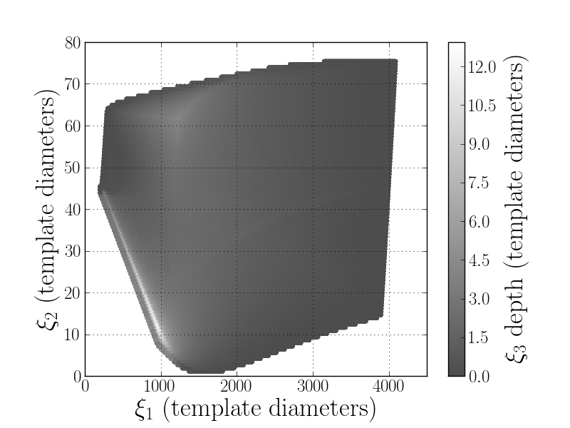
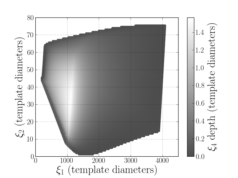
We next construct a bank of template waveforms using the TaylorR2F4 parameter space metric. We begin by exploring the parameter space to assess the effective dimensionality. In Fig. 2 we show the depths of the and directions as a function of and for the TaylorR2F4 parameter space. We immediately notice that the degeneracies present in the TaylorF2 space, which allow us to use a two-dimensional placement, are much weaker in the TaylorR2F4 parameter space. For this space there is substantial depth in the third direction. In one small region it is wider than ten template diameters. The median depth in this direction, however, is only one template diameter.
If the depth in the third direction was larger in all regions, the most efficient placement scheme would be to place a template bank in a three-dimensional lattice Conway and Sloane (1993). However, in regions where the depth of the third direction is small, the three-dimensional lattice, when flattened into the two-dimensional space, would cause an overcoverage. We therefore tried both a three-dimensional lattice placement and a two-dimensional placement, followed by stacking in the third direction as we used for the TaylorF2 bank. Additionally, unlike in the TaylorF2 space, the depth of the fourth dimension is not negligible. However, as in most places the width in that direction is small, the stacking technique can also be used to cover the depth of the fourth dimension when needed.
When we choose to employ a three-dimensional lattice we find that 1,805,036 templates are needed to cover the space, 90,463 of which were added due to stacking in the fourth direction. In contrast, when we use a hexagonal lattice followed by stacking in both the third and fourth directions we find that 1,100,277 templates are needed, of which 741,626 were added by the stacking process. It may seem surprising that the 2D hexagonal lattice requires less templates than the 3D lattice. In fact, it would still require less templates even if the depth of the third direction was large in all regions of the space. The reason for this is that the placement guarantees that all points within the three-dimensional space will have a fitting factor of at least 0.97. With the hexagonal placement followed by stacking, there are points in the space where the fitting factor can be as low as 0.96 (when the depth of the fourth dimension is significant this can be as low as 0.95). If we were to require that all points within the space must have a fitting factor of at least 0.97, our hexagonal lattice would need to be placed to a minimal match of 0.98. For comparison, we generated a three-dimensional lattice with a minimal match of 0.96; this bank contained 1,175,523 templates. The three-dimensional lattice is still less efficient than the two-dimensional lattice. This can be attributed, as described above, to the fact that the depth of the third direction is not large in all areas of the parameter space. In some areas a two-dimensional lattice, without any stacking, is sufficient to cover the parameter space. An alternative approach might be to use a three-dimensional lattice of points only in regions where it is needed and a two-dimensional lattice elsewhere; we did not investigate that here. For the simulations in the following sections, we use the hexagonal lattice with stacking as the method for placing banks of templates for the TaylorT4 approximant.
VII Results I: Validating the new template bank placement for aligned-spin systems
In this section we demonstrate that our aligned-spin template banks achieve the level of coverage they are constructed for when used to search for aligned-spin signals. We also compare our banks to banks generated using a stochastic placement algorithm Harry et al. (2009); Babak (2008); Manca and Vallisneri (2010); Ajith et al. (2012) and show that our method achieves the same level of coverage with fewer templates.
To verify the performance of our aligned-spin template banks we compute the fitting factors between the banks and a set of 100,000 aligned-spin NSBH waveforms. These waveforms are drawn from the distribution that we describe in Sec. II, except that the spins are all aligned (or antialigned) with the orbital angular momentum.
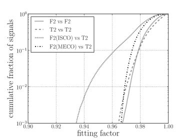
In Fig. 3 we show the results of this test using the template bank constructed with the TaylorF2 metric. We show results when both template waveforms and signals are modeled using the TaylorF2 approximant, when both are modeled using the TaylorT2 approximant and when we model the template waveforms with TaylorF2 and the signals with TaylorT2. In both cases where the same waveform model was used almost all of the fitting factors were greater than 0.97. The bank generation was successful.
The lowest matches in the TaylorF2 vs TaylorF2 results were in cases where a system with low mass ratio was recovered with a template with a high mass ratio, or vice versa. These are systems where the degeneracy between the spins and the mass ratio Baird et al. (2013) causes the phase evolution of the two systems to be very similar and therefore the match predicted by the metric is higher than 0.97. However, the system with the larger black-hole mass will terminate at a significantly lower frequency than the system with the smaller black-hole mass and some power is lost due to the difference in termination frequencies, which is not predicted by the metric.
The difference in termination conditions is also the reason why we see comparatively poorer performance when using TaylorF2 waveforms, terminated at the ISCO frequency, to search for TaylorT2 signals. The TaylorT2 signals terminate when the evolution becomes unphysical, either at the MECO or where the frequency spuriously begins to drop. In some cases, especially when the spins are large, these can correspond to rather different termination frequencies. To demonstrate this we also show the performance of searching for TaylorT2 signals with TaylorF2 waveforms, but where we terminate the TaylorF2 waveforms using the same cutoff frequency that TaylorT2 waveforms would have at the given masses and spins. This gives a much more comparable performance to the TaylorF2 vs TaylorF2 and TaylorT2 vs TaylorT2 cases.
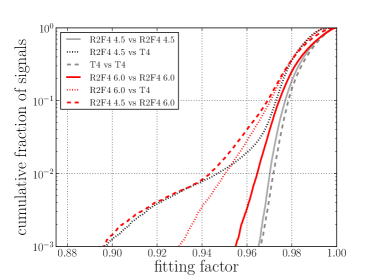
In Fig. 4 we repeat this test using the template bank constructed with the TaylorR2F4 metric, with terms restricted to 4.5PN order. We show results when the template waveforms and signals are modeled with varying approximants. We use TaylorR2F4 with terms up to 4.5PN order, TaylorR2F4 with terms up to 6PN order and TaylorT4. We can see from this figure that using TaylorR2F4 template waveforms with terms only to 4.5PN order would not be satisfactory when conducting searches for signals modeled with the TaylorT4 approximant. However, we note that when this bank is used with either TaylorT4 templates or TaylorR2F4 templates including terms up to 6PN order the coverage is much better. When TaylorT4 is used to model both the signals and the template waveforms we find that of the fitting factors are greater than 0.97. In this plot the TaylorR2F4 waveforms are terminated at the same frequency (the MECO frequency) as the TaylorT4 waveforms.
The TaylorR2F4 metric, with terms up to 4.5PN, is sufficient to place a bank of templates to cover waveforms modeled by the TaylorT4 approximant. However, when performing the matched filtering the templates must be modeled with either TaylorT4 or TaylorR2F4 with terms up to 6PN order.
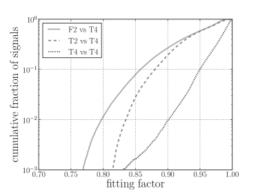
In Fig. 5 we also show the performance of a bank placed using the TaylorF2 metric to search for TaylorT4 aligned-spin signals. We assess the performance when the templates are modeled using TaylorF2, TaylorT2 and TaylorT4 approximants. Even when TaylorT4 is used to model both template waveforms and signals, of signals are recovered with fitting factors smaller than 0.95. The TaylorF2 metric does not achieve the desired coverage for TaylorT4 waveforms. In a companion work we investigate how the disagreement of different waveform families in the NSBH region of parameter space will reduce detection efficiency Nitz et al. (2013).
VII.1 Varying the upper frequency cutoff and comparison with stochastic placement algorithms
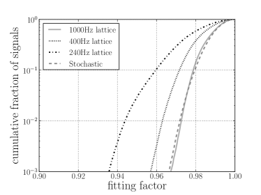
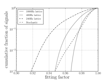
Filtering templates against data from advanced gravitational-wave detectors will require a large amount of computing power. It would therefore be desirable if we could reduce the overcoverage that is incurred in the high-mass region of the parameter space when using an upper frequency cutoff of 1000 Hz. An alternative “stochastic” placement scheme, based on randomly picking points in the space and only retaining points which are not close to points already in the bank Harry et al. (2009); Babak (2008); Manca and Vallisneri (2010), is capable of using an upper frequency cutoff that varies with mass Ajith et al. (2012). However, this method is known to pack templates more densely than a geometrical lattice Harry et al. (2009). We found that using a stochastic method to cover this NSBH space with the same covering criterion required 971,105 (1,327,175) templates when using the TaylorF2 (TaylorR2F4) metric to place the bank. In both cases this is larger than our geometric algorithm using a constant upper frequency cutoff of 1000 Hz. It is also possible to generate the geometric bank with a lower upper frequency cutoff. This will require less templates but will not reach the desired coverage in the lower-mass regions of the parameter space. In Fig. 6 we compare the efficiency of geometric banks placed using a 240, 1000 and 400 Hz upper frequency cutoff. These correspond to roughly the lowest possible ISCO frequency, the highest and an “average” system. The sizes of these banks are shown in Table 1. As expected we notice a number of systems recovered with fitting factors less than 0.97 when the upper frequency cutoff is reduced. We also compare with the performance of a stochastic placement algorithm, which uses a varying upper frequency cutoff. The performance of the stochastic bank is very comparable to the 1000 Hz bank when using the TaylorF2 metric. When using the TaylorR2F4 metric the stochastic bank, which was placed using seed points, seems to be struggling to achieve the necessary coverage in certain regions of the space. As the stochastic placement algorithm only uses a finite number of sample points, it is known that it can leave holes in the parameter space, resulting in undercoverage Harry et al. (2009).
We plan to adapt the geometric placement algorithm to allow the upper frequency cutoff to vary over the space; however, we leave this investigation for future work. We note that the minimal match and lower frequency cutoff of the bank can also be modified to reduce the number of templates and balance the computational cost Keppel (2013).
VIII Results II: Template bank performance when searching for generic NSBH signals
In this section we evaluate the efficiency of searching for generic NSBH systems using template banks of nonspinning waveforms. Template banks of nonspinning waveforms were used to search for NSBH signals in data from LIGO and Virgo’s most recent science runs Abbott et al. (2009a, b); Abadie et al. (2010b, 2012). We demonstrate that ignoring the effects of spin when conducting searches for NSBH systems in the advanced detector era will significantly decrease the rate of NSBH observations and impose a selection bias against systems with large spins and large . We then evaluate the efficiency of searching for generic NSBH systems using our new template bank of aligned-spin waveforms. We calculate the improvement gained by using our new bank when compared to a nonspinning bank.
VIII.1 Performance of nonspinning template banks when searching for generic NSBH signals
We compute fitting factors between a set of 100,000 generic, precessing NSBH signals and a bank of nonspinning template waveforms. The precessing signals are drawn from the distribution that we describe in Sec. II. To mitigate any bias that arises due to the choice of waveform approximant we run the simulation twice. First we use the TaylorT2 approximant for both signal and template waveforms and a template bank designed to obtain a fitting factor of at least 0.97 for any TaylorT2 non-spinning signal. The simulation was then repeated using the TaylorT4 approximant for both signal and template waveforms and a bank designed with the same fitting factor criterion for TaylorT4 signals. These banks were constructed using the methods described to create aligned-spin banks in section VI but with the spins set to 0.
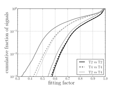
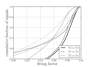
The results of this simulation can be seen in Fig. 7. From this we can calculate the mean and median values of the fitting factor over the signal distribution that we used. The mean fitting factor of the signals is 0.82 (0.84) for the TaylorT2 (TaylorT4) approximant, while the median fitting factor was 0.86 (0.88). In both cases the distributions have long tails, with some systems recovered with less than 30% of their optimal SNR. We also show results where we have modeled the templates using the TaylorT2 approximant and the signals using the TaylorT4 approximant. In this case the mean fitting factor is 0.84 and the median is 0.87. We notice that fewer signals are recovered with high fitting factors () than in the other two cases, but we notice that at lower values of fitting factor the performance is very similar to the TaylorT4 vs TaylorT4 case. The slight improvement of the TaylorT2 vs TaylorT4 case at lower fitting factors can be attributed to the fact that the TaylorT2 bank is larger than the TaylorT4 bank and therefore has more freedom to match TaylorT4-modeled spinning signals.
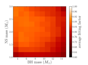
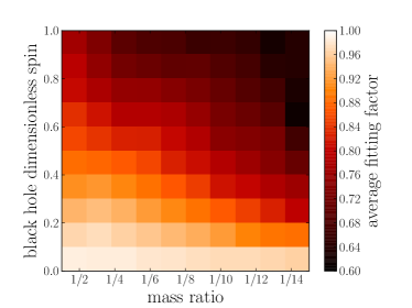
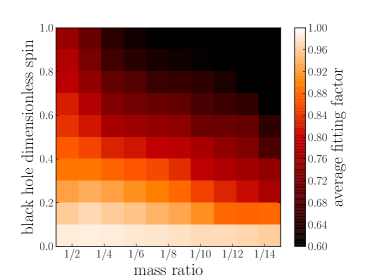
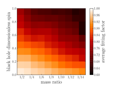
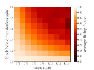
In Fig. 8, we show the mean fitting factor as a function of the intrinsic parameters of the system when both templates and signals were modeled with the TaylorT4 approximant. For comparison, in Fig. 9 we show the mean fitting factor as a function of the spin magnitude and mass ratio for the TaylorT2 vs TaylorT2 results and the TaylorT2 vs TaylorT4 results. In both cases the results are similar to the TaylorT4 vs TaylorT4 case, which indicates that the results are not suffering from a significant bias due to the choice of waveform approximant. However, we note that when using TaylorT2 as the signal model, the performance of the nonspinning banks is worse for high spin, unequal mass systems than when using TaylorT4 as the signal model.
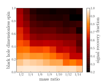
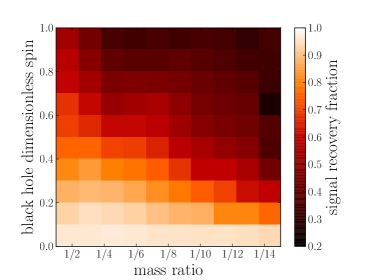
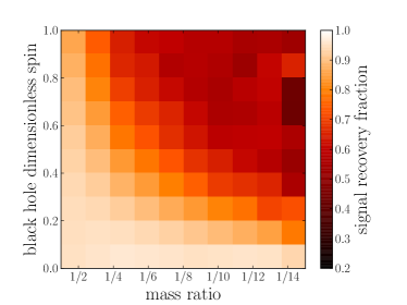
In Fig. 10 we show the signal recovery fraction as a function of the BH spin magnitude and the mass ratio. The signal recovery fraction is defined in Sec. IV. It is clear that using a nonspinning bank to search for NSBH systems will result in a considerable reduction in the NSBH detection rate. In addition, the ability to detect systems with high spin, especially systems that also have unequal masses, is especially poor. We note that these efficiencies would be improved by using nonspinning templates outside of the chosen mass ranges, for example BNS or binary black-hole template waveforms, or even templates with unphysical mass parameters Brown et al. (2012a); Baird et al. (2013).
VIII.2 Performance of aligned-spin template banks when searching for generic NSBH signals
With the template banks of aligned-spin systems described in Sec. VI, we are able to recover aligned-spin systems modeled with either the TaylorT2 or TaylorT4 approximant with fitting factors greater than 0.97 in of cases, as shown in Sec. VII. If we use these banks to search for precessing systems modeled with the same approximants, any loss in signal power, beyond that lost due to the spacing of the aligned-spin bank, is entirely due to precession. We now assess the performance of these aligned-spin banks when searching for generic, precessing NSBH signals and identify regions of the parameter space where precessional effects cause a significant loss in detection rate.
Our signal population is a set of 100,000 precessing NSBH signals. This distribution was described in Sec. II. For comparison this is the same set of signals as we used in Sec. VIII.1. As before, we will assess fitting factors using both the TaylorT2 and TaylorT4 models to mitigate any bias arising from choice of waveform model. When TaylorT2 is used as the signal model, we will use the bank of aligned-spin systems that was placed using the TaylorF2 metric and a 1000 Hz upper frequency cutoff and model the templates using the TaylorT2 approximant. When TaylorT4 is used as the signal model, we will use the bank of aligned-spin systems placed using the TaylorR2F4 metric and model the templates with TaylorT4. The placement of these banks was described in Sec. VI.
The results of these simulations can be seen in Fig. 7, where we also compare with the results obtained in Sec. VIII.1 when using nonspinning template banks. We can clearly see from Fig. 7 that the distribution of fitting factors for the case when both signals and templates were modeled with TaylorT2 agrees well with the case when both were modeled with TaylorT4. This indicates that we have disentangled precessional effects from waveform-dependent effects and our results are free of any bias due to the choice of waveform model. The mismatches seen here, beyond that caused by the discreteness of the bank, are due only to the effects of precession. In both cases we observe a median fitting factor of and a mean fitting factor of . This is a clear improvement over the nonspinning results where the mean fitting factor was 0.82 (0.84) for TaylorT2 (TaylorT4) and the median fitting factor was 0.86 (0.88).
In Fig. 7 we also show results where the template waveforms are modeled with TaylorT2 and the signals are modeled with TaylorT4. In this case the performance is worse, with a median fitting factor of and a mean fitting factor of .
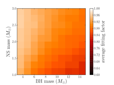
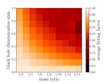
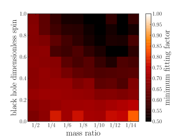
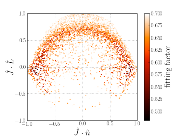
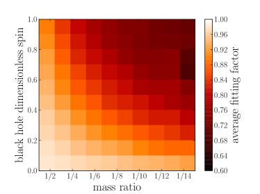
In Fig. 11 we show the mean fitting factor as a function of the intrinsic parameters for our results with the TaylorT4 waveform. We also show the minimum fitting factor and the signal recovery fraction as a function of the BH spin magnitude and mass ratio for the same results. The figure serves to highlight that there are certain systems in certain regions of the parameter space where precessional effects cause the NSBH signals to have large mismatches with a bank of aligned-spin templates. This is most prominent when and the BH spin magnitude are both large, i.e. where the black hole’s angular momentum is particularly large relative to the orbital angular momentum. We explore this further in Fig. 12 where, following the work of Brown et al. (2012b), we show the distribution of precessing systems recovered with fitting factors smaller than . This is plotted as a function of the angles between the total angular momentum, the orbital angular momentum and the line of sight to an observer. As predicted in Brown et al. (2012b), there is clearly a correlation between these angles and the systems recovered with the lowest fitting factors. To demonstrate that these results are not specific to the TaylorT4 waveform, in Fig. 13 we show the mean fitting factor as a function of the BH spin magnitude and mass ratio for our TaylorT2 vs TaylorT2 and TaylorT2 vs TaylorT4 results. The TaylorT2 results are very similar to the TaylorT4 results in Fig. 11. This again demonstrates that the choice of waveform is not affecting our statements regarding the effect precession will have on searches for NSBH signals using aligned-spin template banks. When searching for TaylorT4 signals with TaylorT2 templates we see lower fitting factors. The disagreement between these two waveform models is a significant factor that will affect searches for NSBH systems with second-generation observatories. Computing higher order terms in the Post-Newtonian (PN) expansion of the center-of-mass energy and gravitational wave flux will help to reduce this disagreement and produce waveforms that better match real gravitational-wave signals.
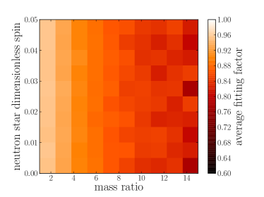
To investigate whether the spin of the neutron star has any effect on these results, in Fig. 14 we plot the average fitting factor as a function of the mass ratio and the neutron-star dimensionless spin. There is not any noticeable correlation between the average fitting factor and the neutron star’s spin. As a further test we generated a template bank of TaylorF2 waveforms, using the same parameters as the banks discussed in Sec. VI and used in this section, except the neutron-star spin was only allowed to take a value of 0. We then evaluated the fitting factor between this bank and a set of TaylorF2 NSBH waveforms using the same distribution as described in Sec. II except both spins were constrained to be aligned with the orbit and the neutron spin was either set to a value of 0.05 or -0.05. We found that 99.99% of these signals had fitting factors larger than 0.96, which is the smallest fitting factor allowed by the placement algorithm. These results indicate that as long as the NS spin is then it will be a negligible factor in searches for NSBH binaries with aLIGO and AdV.
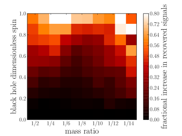
We can also compare these results to the results we obtained using a nonspinning template bank in Sec. VIII.1. In Fig. 15 we show the fractional increase in the number of recovered signals between using nonspinning and aligned-spin template banks for the TaylorT4 approximant. The fractional increase in the number of recovered signals is calculated by taking the ratio of the signal recovery fraction when using a nonspinning bank and the signal recovery fraction when using an aligned-spin bank. This figure helps to emphasize that a much greater fraction of systems with large spin would be recovered when using an aligned-spin template bank. In Table 2 we summarize the average signal recovery fractions for the aligned-spin banks and compare these numbers to the results obtained with nonspinning template banks. We remind the reader that we are comparing signal recovery at a fixed signal-to-noise ratio threshold. Signal recovery at a fixed false-alarm probability will depend on other factors, including the size of the parameter space covered by the template bank and the non-Gaussianity of the data. We discuss this further in the conclusion.
| Template | Signal | Signal recovery fraction for non-spinning bank | Signal recovery fraction for aligned-spin bank | Fractional improvement in signal recovery | |||
| approximant | approximant | Average | Average | Average | |||
| TaylorT2 | TaylorT2 | 64% | 63% | 83% | 74% | 30% | 17% |
| TaylorT4 | TaylorT4 | 69% | 67% | 82% | 73% | 19% | 9% |
| TaylorT2 | TaylorT4 | 67% | 64% | 77% | 67% | 16% | 5% |
Finally, we compare our results with previous works. In Ajith et al. (2012) the authors presented an efficiency study when using a template bank of stochastically generated aligned-spin signals. We verified that when using the stochastic algorithm we used in this work, and using the same set of parameters as the study described in Ajith et al. (2012), we generated a bank with the same number of templates. We have therefore demonstrated that our template bank algorithm requires less templates to achieve the same level of coverage as the algorithm used in Ajith et al. (2012). In that work the effective fitting factor for a NSBH system with masses given by , was estimated to be 0.95, which corresponds to a signal recovery fraction of 86%. In contrast, our results show a lower signal recovery fraction for the same masses of when the same waveform model is used to model both the template and signal. It is not clear why this discrepancy occurs; however, it may be partially explained by the fact that the authors of Ajith et al. (2012) used a lower frequency cutoff in their matched filters of 20 Hz, whereas we used 15 Hz, which is more appropriate for the predicted aLIGO zero-detuned–high-power noise curve.
In Brown et al. (2012b) the authors used a simplified model of precessing systems to predict the distribution of fitting factors for NSBH systems. These results, shown in Fig. 11 of that work, agree qualitatively with the results obtained here. We also obtain quantitative agreement by comparing our simulations of generic precessing systems with TaylorT4 as the signal and template model with the values predicted by Eq. 46b of Brown et al. (2012b). We find that 90% of the fitting factors are within of the predicted values. They also predicted the distribution of the signals that would be recovered with the lowest fitting factors as a function of the orientation of the black-hole spin and the orientation of the orbital plane with respect to the line of sight. We produce a similar distribution in Fig. 12. A further exploration of the agreement of the fitting factors with this prediction will be carried out in a future work making use of these simulations.
IX Conclusions
In this work we have explored the effect that the angular momentum of the black hole will have on searches for neutron-star black-hole binaries with aLIGO. The black hole’s angular momentum will affect the phase evolution of the emitted gravitational-wave signal, and, if the angular momentum is misaligned with the orbital plane, will cause the system to precess. We have found that if these effects are neglected in the filter waveforms used to search for NSBH binaries it will result in a loss in detection rate of when searching for NSBH systems with masses uniformly distributed in the range . When restricting the masses to we find that the loss in detection rate is . The error in these measurements is due to uncertainty in the PN waveform models used to simulate NSBH gravitational-wave signals. In a companion work we investigate how the uncertainty in waveform models used to simulate NSBH waveforms will reduce detection efficiency Nitz et al. (2013).
We have presented a new method to create a template bank of NSBH filter waveforms, where the black hole’s angular momentum is included but is restricted to be (anti)aligned with the orbit. These waveforms will include the effect that the black hole’s angular momentum has on the phase evolution of the gravitational-wave signal, but will not include any precessional effects. We have shown that this bank offers a improvement in the detection rate of neutron-star–black-hole mergers when compared to a nonspinning template bank when searching for NSBH systems with masses in the range . However, when searching for NSBH systems with masses restricted to the range we find the improvement is reduced to . Some systems are not recovered well with this new bank of filters. These systems are ones where the black-hole spin is misaligned with the orbit and the waveform is significantly modified due to precession of the orbital plane. This happens most often when and the spin magnitude are both large. In Brown et al. (2012b) the authors predict where in the parameter space to expect NSBH systems that will not be recovered well by nonprecessing template banks. These predictions were given in terms of the angles between the orbital plane, the black hole’s angular momentum and the line of sight to an observer. These predictions agree with the results that we obtain in this work. In Ajith et al. (2012) the authors claim that an aligned-spin template bank will be effectual for detecting precessing NSBH systems. In this work, we find that with an aligned-spin template bank of NSBH systems will be missed compared to an ideal search with exactly matching filter waveforms. In reality this ideal search could never be performed as it would require an infinite number of filter waveforms. Template banks are usually constructed to allow for no more than a 3% loss in SNR; therefore, we expect to lose up to of systems even if the template bank fully covers the signal parameter space. We therefore conclude that searches using precessing waveforms as templates could potentially increase the detection rate of NSBH signals, but not by more than . Performing such a search would, however, remove an observational bias against systems where precessional effects are most prevalent in the gravitational-wave signal.
These figures are also affected by the parameter distribution chosen for the NSBH systems. Here we chose a distribution that is uniform in mass, uniform in spin magnitudes, isotropic in spin orientations and isotropic in orientation parameters and sky location. We have, however, explored how the ability to detect precessing NSBH signals varies as a function of the masses and spins as seen in Figs. 11 and 12.
When searching for NSBH systems in aLIGO one has to consider the non-Gaussianity of the background noise, which we have not done in this work. A non-Gaussian noise artifact can produce SNRs that are considerably larger than those expected from Gaussian noise fluctuations. To deal with this, numerous consistency tests are used in the analyses to separate gravitational-wave signals from instrumental noise artifacts Babak et al. (2013). It is possible that the detection rate could be further reduced from the values we quote in this work if some signals fail these consistency tests and are misclassified as non-Gaussian noise transients. However, these signal consistency tests should only act to remove, or reduce the significance of, events that already have low fitting factors and therefore do not match well with the search templates. Another important consideration is that of the number of templates used in the bank. To achieve higher fitting factors will require more template waveforms, covering a larger signal space, which will allow more freedom in matching the background noise and will mean that the SNR of the loudest background triggers will increase. Therefore signals will need slightly higher SNRs to achieve the same false-alarm probability. However, a factor of 10 increase in the number of independent templates will only increase the expected SNR of the loudest background event by less than , if Gaussian noise is assumed. Therefore, while we are careful to note these considerations, we do not believe they will have a large impact on the numbers we quote above and leave a detailed investigation of such effects to future work.
In this work we have restricted ourselves to considering post-Newtonian, inspiral-only signal waveforms and consider only the case of two point particles. This was done as there is not currently any widely available waveform model that includes both the full evolution of a NSBH coalescence and includes precessional effects over the full parameter space that we consider. When such a model is available it may be that tidal forces and the merger component of the waveform may affect our conclusions. We believe that such effects will be limited as tidal effects are not expected to be important for detection of NSBH systems with aLIGO Foucart et al. (2013) and merger physics becomes increasingly important at higher masses Brown et al. (2012c); Smith et al. (2013), while we have restricted the black-hole mass to in our simulations. However it would be informative to repeat our simulations when a full NSBH waveform model including tidal and merger physics is available.
Acknowledgements
We thank Stefan Ballmer, Alessandra Buonanno, Eliu Huerta, Prayush Kumar, Richard O’Shaughnessy, B. S. Sathyaprakash, Peter Saulson, Matt West and Karl Wette for useful discussions. We also thank Frank Ohme and the anonymous referee for providing thoughtful and insightful comments on this manuscript. This work is supported by National Science Foundation awards PHY-0847611 (DAB, AHN), PHY-1205835 (AHN, IWH), PHY-0970074 (EO), PHY-0855589 (AL) and PHY11-25915 (DAB,IWH,EO,AL). DAB, IWH, AL, and EO thank the Kavli Institute for Theoretical Physics at Santa Barbara University, supported in part by NSF grant PHY-0551164, for hospitality during this work. DAB thanks the LIGO Laboratory Visitors Program, supported by NSF cooperative agreement PHY-0757058, for hospitality. DK and AL thank the Max Planck Gesellschaft for support. DAB is supported by a Cottrell Scholar award from the Research Corporation for Science Advancement. Computations used in this work were performed on the Syracuse University Gravitation and Relativity cluster, which is supported by NSF awards PHY-1040231 and PHY-1104371.
References
- Aasi et al. (2013) J. Aasi et al. (LIGO Scientific Collaboration, Virgo Collaboration), (2013), arXiv:1304.0670 [gr-qc] .
- Harry et al. (2010) G. M. Harry et al., Class. Quant. Grav. 27, 084006 (2010).
- Acernese et al. (2009) F. Acernese et al., (2009), Virgo Technical Report 0027A-09.
- (4) F. Acernese et al., “Plans for the upgrade of the gravitational wave detector virgo: Advanced virgo,” in The Twelfth Marcel Grossmann Meeting, Chap. 313, pp. 1738–1742.
- Belczynski et al. (2013) K. Belczynski, T. Bulik, I. Mandel, B. Sathyaprakash, A. A. Zdziarski, et al., Astrophys.J. 764, 96 (2013), arXiv:1209.2658 [astro-ph.HE] .
- Abadie et al. (2010a) J. Abadie et al. (LIGO Scientific Collaboration, Virgo Collaboration), Class.Quant.Grav. 27, 173001 (2010a), arXiv:1003.2480 [astro-ph.HE] .
- Cutler et al. (1993) C. Cutler, T. A. Apostolatos, L. Bildsten, L. S. Finn, E. E. Flanagan, et al., Phys.Rev.Lett. 70, 2984 (1993), arXiv:astro-ph/9208005 [astro-ph] .
- Apostolatos et al. (1994) T. A. Apostolatos, C. Cutler, G. J. Sussman, and K. S. Thorne, Phys. Rev. D49, 6274 (1994).
- Kidder et al. (1993) L. E. Kidder, C. M. Will, and A. G. Wiseman, Phys.Rev. D47, 4183 (1993), arXiv:gr-qc/9211025 [gr-qc] .
- Kidder (1995) L. E. Kidder, Phys.Rev. D52, 821 (1995), arXiv:gr-qc/9506022 [gr-qc] .
- Poisson (1998) E. Poisson, Phys.Rev. D57, 5287 (1998), arXiv:gr-qc/9709032 [gr-qc] .
- Mikoczi et al. (2005) B. Mikoczi, M. Vasuth, and L. A. Gergely, Phys.Rev. D71, 124043 (2005), arXiv:astro-ph/0504538 [astro-ph] .
- Nitz et al. (2013) A. H. Nitz, A. Lundgren, D. A. Brown, E. Ochsner, D. Keppel, et al., (2013), arXiv:1307.1757 [gr-qc] .
- Wainstein and Zubakov (1962) L. A. Wainstein and V. D. Zubakov, Extraction of Signals from Noise (Prentice-Hall, Englewood Cliffs, 1962).
- Wainstein and Zubakov (1968) L. A. Wainstein and V. D. Zubakov, Statistical Theory of Signal Detection (Permagon, London, 1968).
- Allen et al. (2012) B. Allen, W. G. Anderson, P. R. Brady, D. A. Brown, and J. D. E. Creighton, Phys.Rev. D85, 122006 (2012), arXiv:gr-qc/0509116 [gr-qc] .
- Peters and Mathews (1963) P. C. Peters and J. Mathews, Phys. Rev. 131, 435 (1963).
- Thorne (1987) K. S. Thorne, in Three hundred years of gravitation, edited by S. Hawking and W. Israel (Cambridge University Press, 1987) pp. 330–458.
- Sathyaprakash and Dhurandhar (1991) B. S. Sathyaprakash and S. V. Dhurandhar, Phys.Rev. D44, 3819 (1991).
- Poisson and Will (1995) E. Poisson and C. M. Will, Phys.Rev. D52, 848 (1995), arXiv:gr-qc/9502040 [gr-qc] .
- Owen (1996) B. J. Owen, Phys.Rev. D53, 6749 (1996), arXiv:gr-qc/9511032 [gr-qc] .
- Owen and Sathyaprakash (1999) B. J. Owen and B. S. Sathyaprakash, Phys.Rev. D60, 022002 (1999), arXiv:gr-qc/9808076 [gr-qc] .
- Babak et al. (2006) S. Babak, R. Balasubramanian, D. Churches, T. Cokelaer, and B. Sathyaprakash, Class.Quant.Grav. 23, 5477 (2006), arXiv:gr-qc/0604037 [gr-qc] .
- Balasubramanian et al. (1996) R. Balasubramanian, B. S. Sathyaprakash, and S. V. Dhurandhar, Phys.Rev. D53, 3033 (1996), arXiv:gr-qc/9508011 [gr-qc] .
- Cokelaer (2007) T. Cokelaer, Phys.Rev. D76, 102004 (2007), arXiv:0706.4437 [gr-qc] .
- Babak et al. (2013) S. Babak, R. Biswas, P. Brady, D. Brown, K. Cannon, et al., Phys.Rev. D87, 024033 (2013), arXiv:1208.3491 [gr-qc] .
- Abbott et al. (2009a) B. P. Abbott et al. (LIGO Scientific Collaboration), Phys. Rev. D79, 122001 (2009a), arXiv:0901.0302 [gr-qc] .
- Abbott et al. (2009b) B. P. Abbott et al. (LIGO Scientific Collaboration), Phys. Rev. D80, 047101 (2009b), arXiv:0905.3710 [gr-qc] .
- Abadie et al. (2010b) J. Abadie et al. (LIGO and Virgo Scientific Collaborations), Phys. Rev. D82, 102001 (2010b), arXiv:1005.4655 [gr-qc] .
- Abadie et al. (2012) J. Abadie et al., Phys.Rev. D85, 082002 (2012), arXiv:1111.7314 [gr-qc] .
- Babak (2008) S. Babak, Class. Quant. Grav. 25, 195011 (2008), arXiv:0801.4070 [gr-qc] .
- Harry et al. (2009) I. W. Harry, B. Allen, and B. S. Sathyaprakash, Phys.Rev. D80, 104014 (2009), arXiv:0908.2090 [gr-qc] .
- Manca and Vallisneri (2010) G. M. Manca and M. Vallisneri, Phys.Rev. D81, 024004 (2010), arXiv:0909.0563 [gr-qc] .
- Ajith et al. (2012) P. Ajith, N. Fotopoulos, S. Privitera, A. Neunzert, and A. Weinstein, (2012), arXiv:1210.6666 [gr-qc] .
- Brown et al. (2012a) D. A. Brown, I. Harry, A. Lundgren, and A. H. Nitz, Phys.Rev. D86, 084017 (2012a), arXiv:1207.6406 [gr-qc] .
- Apostolatos (1996) T. A. Apostolatos, Phys.Rev. D54, 2421 (1996).
- Buonanno et al. (2003) A. Buonanno, Y.-b. Chen, and M. Vallisneri, Phys.Rev. D67, 104025 (2003), arXiv:gr-qc/0211087 [gr-qc] .
- Grandclement et al. (2003) P. Grandclement, V. Kalogera, and A. Vecchio, Phys. Rev. D67, 042003 (2003), arXiv:gr-qc/0207062 .
- Grandclement and Kalogera (2003) P. Grandclement and V. Kalogera, Phys.Rev. D67, 082002 (2003), arXiv:gr-qc/0211075 [gr-qc] .
- Grandclement et al. (2004) P. Grandclement, M. Ihm, V. Kalogera, and K. Belczynski, Phys.Rev. D69, 102002 (2004), arXiv:gr-qc/0312084 [gr-qc] .
- Pan et al. (2004) Y. Pan, A. Buonanno, Y.-b. Chen, and M. Vallisneri, Phys.Rev. D69, 104017 (2004), arXiv:gr-qc/0310034 [gr-qc] .
- Buonanno et al. (2004) A. Buonanno, Y.-b. Chen, Y. Pan, and M. Vallisneri, Phys.Rev. D70, 104003 (2004), arXiv:gr-qc/0405090 [gr-qc] .
- Buonanno et al. (2005) A. Buonanno, Y. Chen, Y. Pan, H. Tagoshi, and M. Vallisneri, Phys.Rev. D72, 084027 (2005), arXiv:gr-qc/0508064 [gr-qc] .
- Abbott et al. (2008) B. Abbott et al. (LIGO Scientific Collaboration), Phys. Rev. D78, 042002 (2008), arXiv:0712.2050 [gr-qc] .
- Van Den Broeck et al. (2009) C. Van Den Broeck, D. A. Brown, T. Cokelaer, I. Harry, G. Jones, et al., Phys.Rev. D80, 024009 (2009), arXiv:0904.1715 [gr-qc] .
- Fazi (2009) D. Fazi, Development of a physical-template search for gravitational waves from spinning compact-object binaries with LIGO, Ph.D. thesis, Università di Bologna (2009).
- Harry and Fairhurst (2011) I. Harry and S. Fairhurst, Class.Quant.Grav. 28, 134008 (2011), arXiv:1101.1459 [gr-qc] .
- Brown et al. (2012b) D. A. Brown, A. Lundgren, and R. O’Shaughnessy, Phys.Rev. D86, 064020 (2012b), arXiv:1203.6060 [gr-qc] .
- Lundgren and O’Shaughnessy (2013) A. Lundgren and R. O’Shaughnessy, (2013), arXiv:1304.3332 [gr-qc] .
- Duez (2010) M. D. Duez, Class.Quant.Grav. 27, 114002 (2010), arXiv:0912.3529 [astro-ph.HE] .
- Shibata and Taniguchi (2011) M. Shibata and K. Taniguchi, Living Rev.Rel. 14, 6 (2011).
- Pannarale (2012) F. Pannarale, (2012), arXiv:1208.5869 [gr-qc] .
- Lackey et al. (2013) B. D. Lackey, K. Kyutoku, M. Shibata, P. R. Brady, and J. L. Friedman, (2013), arXiv:1303.6298 [gr-qc] .
- Foucart et al. (2013) F. Foucart, L. Buchman, M. D. Duez, M. Grudich, L. E. Kidder, et al., (2013), arXiv:1307.7685 [gr-qc] .
- Brown et al. (2012c) D. A. Brown, P. Kumar, and A. H. Nitz, (2012c), arXiv:1211.6184 [gr-qc] .
- Smith et al. (2013) R. J. E. Smith, I. Mandel, and A. Vecchio, Phys.Rev. D88, 044010 (2013), arXiv:1302.6049 [astro-ph.HE] .
- Ozel et al. (2010) F. Ozel, D. Psaltis, R. Narayan, and J. E. McClintock, Astrophys.J. 725, 1918 (2010), arXiv:1006.2834 [astro-ph.GA] .
- Farr et al. (2011) W. M. Farr, N. Sravan, A. Cantrell, L. Kreidberg, C. D. Bailyn, et al., Astrophys.J. 741, 103 (2011), arXiv:1011.1459 [astro-ph.GA] .
- Kreidberg et al. (2012) L. Kreidberg, C. D. Bailyn, W. M. Farr, and V. Kalogera, Astrophys.J. 757, 36 (2012), arXiv:1205.1805 [astro-ph.HE] .
- Prestwich et al. (2007) A. Prestwich, R. Kilgard, P. Crowther, S. Carpano, A. Pollock, et al., Astrophys.J. 669, L21 (2007), arXiv:0709.2892 [astro-ph] .
- Silverman and Filippenko (2008) J. M. Silverman and A. V. Filippenko, Astrophys.J. 678, L17 (2008), arXiv:0802.2716 [astro-ph] .
- Miller et al. (2009) J. Miller, C. Reynolds, A. Fabian, G. Miniutti, and L. Gallo, Astrophys.J. 697, 900 (2009), arXiv:0902.2840 [astro-ph.HE] .
- Ozel et al. (2012) F. Ozel, D. Psaltis, R. Narayan, and A. S. Villarreal, Astrophys.J. 757, 55 (2012), arXiv:1201.1006 [astro-ph.HE] .
- Kiziltan et al. (2010) B. Kiziltan, A. Kottas, and S. E. Thorsett, (2010), arXiv:1011.4291 [astro-ph.GA] .
- Freire et al. (2007) P. C. C. Freire, S. M. Ransom, S. Begin, I. H. Stairs, J. W. Hessels, et al., Astrophys.J. (2007), arXiv:0711.0925 [astro-ph] .
- Rhoades and Ruffini (1974) J. Rhoades, Clifford E. and R. Ruffini, Phys.Rev.Lett. 32, 324 (1974).
- Lo and Lin (2011) K.-W. Lo and L.-M. Lin, Astrophys.J. 728, 12 (2011), arXiv:1011.3563 [astro-ph.HE] .
- Lorimer (2008) D. Lorimer, Living Rev.Rel. 11, 8 (2008), arXiv:0811.0762 [astro-ph] .
- Mandel and O’Shaughnessy (2010) I. Mandel and R. O’Shaughnessy, Class.Quant.Grav. 27, 114007 (2010), arXiv:0912.1074 [astro-ph.HE] .
- Bildsten et al. (1997) L. Bildsten, D. Chakrabarty, J. Chiu, M. H. Finger, D. T. Koh, et al., Astrophys J. Supp. 113, 367 (1997), arXiv:astro-ph/9707125 [astro-ph] .
- Chakrabarty (2008) D. Chakrabarty, AIP Conference Series American Institute of Physics Conference Series, 1068, 67 (2008), arXiv:0809.4031 [astro-ph] .
- Burgay et al. (2003) M. Burgay et al., Nature 426, 531 (2003).
- Damour et al. (2001) T. Damour, B. R. Iyer, and B. S. Sathyaprakash, Phys. Rev. D63, 044023 (2001), arXiv:gr-qc/0010009 .
- Peters (1964) P. Peters, Phys.Rev. 136, B1224 (1964).
- Arun et al. (2009) K. G. Arun, A. Buonanno, G. Faye, and E. Ochsner, Phys. Rev. D79, 104023 (2009), arXiv:0810.5336 [gr-qc] .
- Buonanno et al. (2009) A. Buonanno, B. R. Iyer, E. Ochsner, Y. Pan, and B. S. Sathyaprakash, Phys. Rev. D80, 084043 (2009), arXiv:0907.0700 [gr-qc] .
- Wiseman (1993) A. G. Wiseman, Phys.Rev. D48, 4757 (1993).
- Blanchet et al. (1995a) L. Blanchet, T. Damour, and B. R. Iyer, Phys.Rev. D51, 5360 (1995a), arXiv:gr-qc/9501029 [gr-qc] .
- Blanchet et al. (1995b) L. Blanchet, T. Damour, B. R. Iyer, C. M. Will, and A. G. Wiseman, Phys.Rev.Lett. 74, 3515 (1995b), arXiv:gr-qc/9501027 [gr-qc] .
- Blanchet et al. (1996) L. Blanchet, B. R. Iyer, C. M. Will, and A. G. Wiseman, Class.Quant.Grav. 13, 575 (1996), arXiv:gr-qc/9602024 [gr-qc] .
- Blanchet et al. (2002) L. Blanchet, G. Faye, B. R. Iyer, and B. Joguet, Phys.Rev. D65, 061501 (2002), arXiv:gr-qc/0105099 [gr-qc] .
- Blanchet et al. (2004) L. Blanchet, T. Damour, G. Esposito-Farese, and B. R. Iyer, Phys.Rev.Lett. 93, 091101 (2004), arXiv:gr-qc/0406012 [gr-qc] .
- Blanchet et al. (2012) L. Blanchet, A. Buonanno, and G. Faye, (2012), arXiv:1210.0764 [gr-qc] .
- Bohe et al. (2013) A. Bohe, S. Marsat, and L. Blanchet, (2013), arXiv:1303.7412 [gr-qc] .
- Cutler and Flanagan (1994) C. Cutler and E. E. Flanagan, Phys.Rev. D49, 2658 (1994), arXiv:gr-qc/9402014 [gr-qc] .
- Droz et al. (1999) S. Droz, D. J. Knapp, E. Poisson, and B. J. Owen, Phys.Rev. D59, 124016 (1999), arXiv:gr-qc/9901076 [gr-qc] .
- Blanchet (2006) L. Blanchet, Living Rev.Rel. 9 (2006).
- Apostolatos (1995) T. A. Apostolatos, Phys.Rev. D52, 605 (1995).
- Ohme et al. (2013) F. Ohme, A. B. Nielsen, D. Keppel, and A. Lundgren, (2013), arXiv:1304.7017 [gr-qc] .
- Conway and Sloane (1993) J. Conway and N. Sloane, Sphere Packings, Lattices and Groups, 2nd ed. (Springer-Verlag, New York, 1993).
- Baird et al. (2013) E. Baird, S. Fairhurst, M. Hannam, and P. Murphy, Phys.Rev. D87, 024035 (2013), arXiv:1211.0546 [gr-qc] .
- Keppel (2013) D. Keppel, (2013), arXiv:1303.2005 [physics.data-an] .