CERN-PH-TH-2013-166 FTUAM-13-20 IFT-UAM/CSIC-13-082 RM3-TH/13-9

Investigating the near-criticality
of the Higgs boson

Dario Buttazzoa,b, Giuseppe Degrassic, Pier Paolo Giardinoa,d,
Gian F. Giudicea, Filippo Salab,e, Alberto Salviob,f, Alessandro Strumiad

(a) CERN, Theory Division, Geneva, Switzerland
(b) Scuola Normale Superiore and INFN, sezione di Pisa, Italy
(c) Dipartimento di Matematica e Fisica, Università di Roma Tre and
INFN sezione di Roma Tre, Italy
(d) Dipartimento di Fisica, Università di Pisa and INFN, sezione di Pisa, Italy
(e) Theoretical Physics Group, Lawrence Berkeley National Laboratory, Berkeley, CA, USA
(f) Departamento de Física Teórica, Universidad Autónoma de Madrid
and Instituto de Física Teórica IFT-UAM/CSIC, Madrid, Spain


Abstract

We extract from data the parameters of the Higgs potential, the top Yukawa coupling and the electroweak gauge couplings with full 2-loop NNLO precision, and we extrapolate the SM parameters up to large energies with full 3-loop NNLO RGE precision. Then we study the phase diagram of the Standard Model in terms of high-energy parameters, finding that the measured Higgs mass roughly corresponds to the minimum values of the Higgs quartic and top Yukawa and the maximum value of the gauge couplings allowed by vacuum metastability. We discuss various theoretical interpretations of the near-criticality of the Higgs mass.

1 Introduction

The discovery of the Higgs boson [1, 2] was expected to be the herald of new physics soon to be found at the TeV scale. So far, however, no signal of new physics nor any clear deviation from the SM Higgs properties have been detected at the LHC. Moreover, the Higgs mass has not provided unambiguous indications for new physics. The measured value Mh=125.15±0.24GeVsubscript𝑀plus-or-minus125.150.24GeVM_{h}=125.15\pm 0.24~{}\,{\rm GeV} [3] is a bit high for supersymmetry and a bit low for composite models, making theoretical interpretations rather uncomfortable. Neither option is unequivocally favoured, although neither option is excluded. On the other hand, Mh=125.15±0.24GeVsubscript𝑀plus-or-minus125.150.24GeVM_{h}=125.15\pm 0.24~{}\,{\rm GeV} lies well within the parameter window in which the SM can be extrapolated all the way up to the Planck mass MPlsubscript𝑀PlM_{\rm Pl}, with no problem of consistency other than remaining in the dark about naturalness. Remarkably, in the context of the SM the measured value of Mhsubscript𝑀M_{h} is special because it corresponds to a near-critical situation in which the Higgs vacuum does not reside in the configuration of minimal energy, but in a metastable state close to a phase transition [4] (for earlier considerations see [5, 6, 7, 8, 9, 10, 11, 12, 13, 14, 15, 16, 17, 18, 19, 20, 21, 22, 23, 24, 25, 26, 27]; for related studies see [28, 29, 30, 31, 32, 33, 34, 35, 36, 37, 38, 39, 40, 41, 42, 43, 44, 45, 46, 47, 48, 49, 50, 51, 52]).

We believe that near-criticality of the SM vacuum is the most important message we have learnt so far from experimental data on the Higgs boson. Near-criticality gives us a unique opportunity to obtain information about physics taking place at energy scales well beyond the reach of any collider experiment. Its consequences are so intriguing and potentially so revolutionary that they deserve accurate calculations and dedicated studies. In this paper we continue our programme of investigating the status and implications of near-criticality. We make advancements on both sides: on the computational side, we improve the calculation of the large-field extrapolation of the Higgs potential and of the critical value of Mhsubscript𝑀M_{h} for absolute stability; on the interpretation side, we explore the significance of near-criticality in terms of high-energy SM parameters.

The main new calculations presented in this paper are the results for the ms¯¯ms\overline{\mbox{\sc ms}} quartic Higgs coupling λ(μ¯)𝜆¯𝜇\lambda(\bar{\mu}), for the top Yukawa coupling yt(μ¯)subscript𝑦𝑡¯𝜇y_{t}(\bar{\mu}), for the electroweak gauge couplings at NNLO precision (two loops) in terms of physical observables: the pole masses of the Higgs (Mhsubscript𝑀M_{h}), of the top (Mtsubscript𝑀𝑡M_{t}), of the Z𝑍Z (MZsubscript𝑀𝑍M_{Z}), of the W𝑊W (MWsubscript𝑀𝑊M_{W}), the ms¯¯ms\overline{\mbox{\sc ms}} strong coupling α3(MZ)subscript𝛼3subscript𝑀𝑍\alpha_{3}(M_{Z}), and the Fermi constant Gμsubscript𝐺𝜇G_{\mu}. We improve on the study in ref. [4] where 2-loop threshold corrections to λ(μ¯)𝜆¯𝜇\lambda(\bar{\mu}) had been computed in the limit of vanishing weak gauge couplings, and 2-loop electroweak threshold corrections to yt(μ¯)subscript𝑦𝑡¯𝜇y_{t}(\bar{\mu}) had been neglected. As a byproduct of our two-loop calculation of λ(μ¯)𝜆¯𝜇\lambda(\bar{\mu}) we also obtain the ms¯¯ms\overline{\mbox{\sc ms}} quadratic Higgs coupling m2(μ¯)superscript𝑚2¯𝜇m^{2}(\bar{\mu}) at the NNLO level.

Recently, many authors have contributed towards the completion of the calculation of the renormalisation-group (RG) evolution (β𝛽\beta-functions and thresholds) of the sizeable SM couplings at NNLO precision. We summarise the present status of these calculations in table 1. Our new calculation of threshold corrections, together with the results collected in table 1, allows us to refine the determination of the critical value of Mhsubscript𝑀M_{h} that ensures absolute vacuum stability within the Standard Model (SM) up to the Planck scale. Furthermore, our precision extrapolation of the SM to high energy scales is relevant for testing any new physics scenario able of making predictions, such as unification of gauge couplings constants, or high-scale supersymmetric models that restrict or predict the quartic Higgs coupling.

The paper is organised as follows. In section 2 we outline the general strategy for the two-loop computations and describe our new results. In section 3 we present numerical results for the ms¯¯ms\overline{\mbox{\sc ms}} couplings at the weak scale. The implications of these results for Planck scale physics are discussed in sections 46. The results are summarised in the conclusions. We complemented the paper with several appendices where we collect all the known results on the RG equations and the threshold corrections that we used in our computation.

Renormalisation Group Equations
LO NLO NNLO NNNLO
1 loop 2 loop 3 loop 4 loop
g3subscript𝑔3g_{3} full [53, 54] 𝒪(α32)𝒪superscriptsubscript𝛼32{\cal O}(\alpha_{3}^{2}) [55, 56] 𝒪(α33)𝒪superscriptsubscript𝛼33{\cal O}(\alpha_{3}^{3}) [57, 58] 𝒪(α34)𝒪superscriptsubscript𝛼34{\cal O}(\alpha_{3}^{4}) [59, 60]
𝒪(α3α1,2)𝒪subscript𝛼3subscript𝛼12{\cal O}(\alpha_{3}\alpha_{1,2}) [61] 𝒪(α32αt)𝒪superscriptsubscript𝛼32subscript𝛼𝑡{\cal O}(\alpha_{3}^{2}\alpha_{t}) [62]
full [63] full [64, 65]
g1,2subscript𝑔12g_{1,2} full [53, 54] full [63] full [64, 65]
ytsubscript𝑦𝑡y_{t} full [66] 𝒪(αt2,α3αt)𝒪superscriptsubscript𝛼𝑡2subscript𝛼3subscript𝛼𝑡{\cal O}(\alpha_{t}^{2},\alpha_{3}\alpha_{t}) [67] full [68, 69]
full [70]
λ,m2𝜆superscript𝑚2\lambda,m^{2} full [66] full [71, 72] full [73, 74]
Threshold corrections at the weak scaleabsent{}^{\phantom{X^{X}}}
LO NLO NNLO NNNLO
0 loop 1 loop 2 loop 3 loop
g2subscript𝑔2g_{2} 2MW/V2subscript𝑀𝑊𝑉2M_{W}/V full [75, 76] full [This work]
gYsubscript𝑔𝑌g_{Y} 2MZ2MW2/V2superscriptsubscript𝑀𝑍2superscriptsubscript𝑀𝑊2𝑉2\sqrt{M_{Z}^{2}-M_{W}^{2}}/V full [75, 76] full [This work]
ytsubscript𝑦𝑡y_{t} 2Mt/V2subscript𝑀𝑡𝑉\sqrt{2}M_{t}/V 𝒪(α3)𝒪subscript𝛼3{\cal O}(\alpha_{3}) [77] 𝒪(α32,α3α1,2)𝒪superscriptsubscript𝛼32subscript𝛼3subscript𝛼12{\cal O}(\alpha_{3}^{2},\alpha_{3}\alpha_{1,2}) [34] 𝒪(α33)𝒪superscriptsubscript𝛼33{\cal O}(\alpha_{3}^{3}) [78, 79, 80]
𝒪(α)𝒪𝛼{\cal O}(\alpha) [82] full [This work]
λ𝜆\lambda Mh2/2V2superscriptsubscript𝑀22superscript𝑉2M_{h}^{2}/2V^{2} full [83] for g1,2=0subscript𝑔120g_{1,2}=0 [4]
full [This work]
m2superscript𝑚2m^{2} Mh2superscriptsubscript𝑀2M_{h}^{2} full [83] full [This work]
Table 1: Present status of higher-order computations included in our code. With the present paper the calculation of the SM parameters at NNLO precision is complete. Here we have defined V(2Gμ)1/2𝑉superscript2subscript𝐺𝜇12V\equiv(\sqrt{2}G_{\mu})^{-1/2} and g1=5/3gYsubscript𝑔153subscript𝑔𝑌g_{1}=\sqrt{5/3}g_{Y}.

2 Computing the ms¯¯ms\overline{\mbox{\sc ms}} parameters with two-loop accuracy

In this section we first outline the general strategy followed to determine the ms¯¯ms\overline{\mbox{\sc ms}} parameters in terms of physical observables at the two-loop level. Then, in sects. 2.1 and 2.2, we will discuss the results for the quartic and quadratic Higgs couplings, respectively, while section 2.3 is dedicated to the calculation of two-loop threshold corrections to the top Yukawa coupling.

First of all, all ms¯¯ms\overline{\mbox{\sc ms}} parameters have gauge-invariant renormalisation group equations [84] and are gauge invariant, as we now prove.111Gauge invariance of fermion pole masses has been proved in refs. [85, 86, 87] and here we generalise their proof. Let us consider a generic ms¯¯ms\overline{\mbox{\sc ms}} coupling θ𝜃\theta measuring the strength of a gauge invariant term in the Lagrangian and a generic gauge fixing parametrized by ξ𝜉\xi (for example the Rξsubscript𝑅𝜉R_{\xi} gauges). Let us first recall the definition of θ𝜃\theta in terms of the bare coupling θ0subscript𝜃0\theta_{0},

μ¯d4θ0=k=0ck(θ,ξ)(d4)k,superscript¯𝜇𝑑4subscript𝜃0superscriptsubscript𝑘0subscript𝑐𝑘𝜃𝜉superscript𝑑4𝑘\bar{\mu}^{d-4}\theta_{0}=\sum_{k=0}^{\infty}\frac{c_{k}(\theta,\xi)}{(d-4)^{k}}, (1)

where the cksubscript𝑐𝑘c_{k} are defined to be the residues at the divergence d=4𝑑4d=4. The important point is that c0=θsubscript𝑐0𝜃c_{0}=\theta, with no dependence on ξ𝜉\xi. Since θ0subscript𝜃0\theta_{0} is gauge independent, we have

0=μ¯d4dθ0dξ=dθdξ+k=11(d4)kdck(θ,ξ)dξ.0superscript¯𝜇𝑑4𝑑subscript𝜃0𝑑𝜉𝑑𝜃𝑑𝜉superscriptsubscript𝑘11superscript𝑑4𝑘𝑑subscript𝑐𝑘𝜃𝜉𝑑𝜉0=\bar{\mu}^{d-4}\frac{d\theta_{0}}{d\xi}=\frac{d\theta}{d\xi}+\sum_{k=1}^{\infty}\frac{1}{(d-4)^{k}}\frac{dc_{k}(\theta,\xi)}{d\xi}. (2)

Since this equation is valid for any d𝑑d, and θ𝜃\theta has no poles at d=4𝑑4d=4 by definition, we obtain dθ/dξ=0𝑑𝜃𝑑𝜉0d\theta/d\xi=0, that is θ𝜃\theta is gauge invariant (as well as all the residues cksubscript𝑐𝑘c_{k}).222Notice that this proof does not apply to the Higgs vev v𝑣v, because it is not the coefficient of a gauge-invariant term in the Lagrangian.


To determine the ms¯¯ms\overline{\mbox{\sc ms}} parameters in terms of physical observables two strategies can be envisaged.

  • i)

    Perform an ms¯¯ms\overline{\mbox{\sc ms}} renormalisation to obtain directly the ms¯¯ms\overline{\mbox{\sc ms}} quantity of interest in terms of ms¯¯ms\overline{\mbox{\sc ms}} parameters. Then express the ms¯¯ms\overline{\mbox{\sc ms}} parameters in terms of the physical ones via appropriately derived two-loop relations.

  • ii)

    Use a renormalisation scheme in which the renormalised parameters are directly expressed in terms of physical observables (we call this scheme generically on-shell (OS) and label quantities in this scheme with an OSOS{\rm OS}). Then relate the parameters as expressed in the OS scheme to their ms¯¯ms\overline{\mbox{\sc ms}} counterparts we are looking for.

This last step can be easily done using the relation

θ0=θOSδθOS=θ(μ¯)δθms¯subscript𝜃0subscript𝜃OS𝛿subscript𝜃OS𝜃¯𝜇𝛿subscript𝜃¯ms\theta_{0}=\theta_{\rm OS}-\delta\theta_{\rm OS}=\theta(\bar{\mu})-{\delta\theta}_{\overline{\mbox{\sc ms}}} (3)

or

θ(μ¯)=θOSδθOS+δθms¯,𝜃¯𝜇subscript𝜃OS𝛿subscript𝜃OS𝛿subscript𝜃¯ms\theta(\bar{\mu})=\theta_{\rm OS}-\delta\theta_{\rm OS}+{\delta\theta}_{\overline{\mbox{\sc ms}}}\,, (4)

where θ0subscript𝜃0\theta_{0} is the bare parameter, θ(μ¯)𝜃¯𝜇\theta(\bar{\mu}) (θOSsubscript𝜃OS\theta_{\rm OS}) is the renormalised ms¯¯ms\overline{\mbox{\sc ms}} (OS) version and δθms¯𝛿subscript𝜃¯ms\delta\theta_{\overline{\mbox{\sc ms}}} (δθOS𝛿subscript𝜃OS\delta\theta_{{\rm OS}}) the corresponding counterterm. By definition δθms¯𝛿subscript𝜃¯ms\delta\theta_{\overline{\mbox{\sc ms}}} subtracts only the terms proportional to powers of 1/ϵ1italic-ϵ1/\epsilon and γln(4π)𝛾4𝜋\gamma-\ln(4\pi) in dimensional regularisation, with d=42ϵ𝑑42italic-ϵd=4-2\,\epsilon being the space-time dimension. Concerning the structure of the 1/ϵ1italic-ϵ1/\epsilon poles in the OS and ms¯¯ms\overline{\mbox{\sc ms}} counterterms, one notices that it should be identical once the poles in the OS counterterms are expressed in terms of ms¯¯ms\overline{\mbox{\sc ms}} quantities. Then, after this operation is performed, the desired θ(μ¯)𝜃¯𝜇\theta(\bar{\mu}) is obtained from

θ(μ¯)=θOSδθOS|fin+Δθ,𝜃¯𝜇subscript𝜃OSevaluated-at𝛿subscript𝜃OSfinsubscriptΔ𝜃\theta(\bar{\mu})=\theta_{\rm OS}-\left.\delta\theta_{\rm OS}\right|_{\rm fin}+\Delta_{\theta}, (5)

where the subscript ‘fin’ denotes the finite part of the quantity involved and ΔΔ\Delta is the two-loop finite contribution that is obtained when the OS parameters entering the 1/ϵitalic-ϵ\epsilon pole in the OS counterterm are expressed in terms of ms¯¯ms\overline{\mbox{\sc ms}} quantities, the finite contribution coming from the 𝒪(ϵ)𝒪italic-ϵ{\cal O}(\epsilon) part of the shifts.

MW=80.384±0.014GeVPole mass of the W boson[88]MZ=91.1876±0.0021GeVPole mass of the Z boson[89]Mh=125.15±0.24GeVPole mass of the higgs[3]Mt=173.34±0.76±0.3GeVPole mass of the top quark[90]V(2Gμ)1/2=246.21971±0.00006GeVFermi constant for μ decay[91]α3(MZ)=0.1184±0.0007ms¯ gauge SU(3)c coupling (5 flavours)[92]subscript𝑀𝑊plus-or-minus80.3840.014GeVPole mass of the W boson[88]subscript𝑀𝑍plus-or-minus91.18760.0021GeVPole mass of the Z boson[89]subscript𝑀plus-or-minus125.150.24GeVPole mass of the higgs[3]subscript𝑀𝑡plus-or-minus173.340.760.3GeVPole mass of the top quark[90]𝑉superscript2subscript𝐺𝜇12plus-or-minus246.219710.00006GeVFermi constant for μ decay[91]subscript𝛼3subscript𝑀𝑍plus-or-minus0.11840.0007ms¯ gauge SU(3)c coupling (5 flavours)[92]\begin{array}[]{rcllr}M_{W}&=&80.384\pm 0.014\,\,{\rm GeV}&\hbox{Pole mass of the $W$ boson}&\hbox{\cite[cite]{[\@@bibref{}{Wmass}{}{}]}}\\ M_{Z}&=&91.1876\pm 0.0021\,\,{\rm GeV}&\hbox{Pole mass of the $Z$ boson}&\hbox{\cite[cite]{[\@@bibref{}{Zmass}{}{}]}}\\ M_{h}&=&125.15\pm 0.24~{}\,{\rm GeV}&\hbox{Pole mass of the higgs}&\hbox{\cite[cite]{[\@@bibref{}{HiggsMass}{}{}]}}\\ M_{t}&=&173.34\pm 0.76\pm 0.3\,\,{\rm GeV}&\hbox{Pole mass of the top quark}&\hbox{\cite[cite]{[\@@bibref{}{topmass}{}{}]}}\\ V\equiv(\sqrt{2}G_{\mu})^{-1/2}&=&246.21971\pm 0.00006\,{\rm GeV}&\hbox{Fermi constant for $\mu$ decay}&\hbox{\cite[cite]{[\@@bibref{}{MuLan}{}{}]}}\\ \alpha_{3}(M_{Z})&=&0.1184\pm 0.0007&\hbox{$\overline{\mbox{\sc ms}}$ gauge SU(3)${}_{c}$ coupling (5~{}flavours)}&\hbox{\cite[cite]{[\@@bibref{}{alpha3}{}{}]}}\end{array}
Table 2: Input values of the SM observables used to fix the SM fundamental parameters λ,m,yt,g2,gY𝜆𝑚subscript𝑦𝑡subscript𝑔2subscript𝑔𝑌\lambda,m,y_{t},g_{2},g_{Y}. The pole top mass, Mtsubscript𝑀𝑡M_{t}, is a naive average of TeVatron, CMS, ATLAS measurements, all extracted from difficult MonteCarlo modellings of top decay and production in hadronic collisions. Furthermore, Mtsubscript𝑀𝑡M_{t} is also affected by a non-perturbative theoretical uncertainty of order ΛQCDsubscriptΛQCD\Lambda_{\rm QCD}, that we quantify as ±0.3GeVplus-or-minus0.3GeV\pm 0.3\,{\rm GeV}. Throughout the paper we give explicitly the dependence of all physical quantities on Mtsubscript𝑀𝑡M_{t}, and thus the impact of larger theoretical uncertainties on the top mass is always manifest in our results.

In the following we adopt strategy ii).

The quantities of interests are θ=(m2,λ,v,yt,g2,g1)𝜃superscript𝑚2𝜆𝑣subscript𝑦𝑡subscript𝑔2subscript𝑔1\theta=(m^{2},\lambda,v,y_{t},g_{2},g_{1}), i.e. the quadratic and quartic couplings in the Higgs potential, the vacuum expectation value (vev), the top Yukawa coupling, the SU(2)LSUsubscript2𝐿{\rm SU}(2)_{L} and U(1)YUsubscript1𝑌{\rm U}(1)_{Y} gauge couplings g2subscript𝑔2g_{2} and gYsubscript𝑔𝑌g_{Y} (with g1=5/3gYsubscript𝑔153subscript𝑔𝑌g_{1}=\sqrt{5/3}g_{Y} being the hypercharge coupling rewritten in SU(5) normalisation), and are directly determined in terms of the pole masses of the Higgs (Mhsubscript𝑀M_{h}), of the top (Mtsubscript𝑀𝑡M_{t}), of the Z𝑍Z (MZsubscript𝑀𝑍M_{Z}), of the W𝑊W (MWsubscript𝑀𝑊M_{W}), the Fermi constant Gμsubscript𝐺𝜇G_{\mu} and the ms¯¯ms\overline{\mbox{\sc ms}} strong coupling α3(MZ)subscript𝛼3subscript𝑀𝑍\alpha_{3}(M_{Z}). Their input values are listed in Table 2. Then, using eq. (5), the ms¯¯ms\overline{\mbox{\sc ms}} quantities are obtained. We notice that the weak-scale values for the ms¯¯ms\overline{\mbox{\sc ms}} gauge couplings at the scale μ¯¯𝜇\bar{\mu} are given in terms of Gμ,MWsubscript𝐺𝜇subscript𝑀𝑊G_{\mu},\,M_{W} and MZsubscript𝑀𝑍M_{Z} and not in terms of the fine structure constant and the weak mixing angle at the MZsubscript𝑀𝑍M_{Z} scale as usually done.

In order to fix the notation we write the classical Higgs potential as (the subscript 00 indicates a bare quantity)

V0=m022|H0|2+λ0|H0|4.subscript𝑉0subscriptsuperscript𝑚202superscriptsubscript𝐻02subscript𝜆0superscriptsubscript𝐻04V_{0}=-\frac{m^{2}_{0}}{2}|H_{0}|^{2}+\lambda_{0}|H_{0}|^{4}\ . (6)

The classical Higgs doublet H0subscript𝐻0H_{0} is defined by

H0=(χ(v0+h+iη)/2)subscript𝐻0𝜒subscript𝑣0𝑖𝜂2\begin{array}[]{c}H_{0}=\left(\begin{array}[]{c}\chi\\ (v_{0}+h+i\,\eta)/\sqrt{2}\end{array}\right)\end{array} (7)

in terms of the physical Higgs field hh, and of the neutral and charged would-be Goldstone bosons η𝜂\eta and χ𝜒\chi. The renormalisation of the Higgs potential, eq. (6), was discussed at the one-loop level in [83] and extended at the two-loop level in [4]. We refer to these papers for details. We recall that in ref. [4] the renormalised vacuum is identified with the minimum of the radiatively corrected potential333 This condition is enforced choosing the tadpole counterterm to cancel completely the tadpole graphs. and it is defined through Gμsubscript𝐺𝜇G_{\mu}. Writing the relation between the Fermi constant and the bare vacuum as

Gμ2=12v02(1+Δr0),subscript𝐺𝜇212superscriptsubscript𝑣021Δsubscript𝑟0\frac{G_{\mu}}{\sqrt{2}}=\frac{1}{2v_{0}^{2}}(1+\Delta r_{\scriptscriptstyle 0})\,, (8)

one gets

vOS2=12Gμ,δvOS2=Δr02Gμ.formulae-sequencesuperscriptsubscript𝑣OS212subscript𝐺𝜇𝛿subscriptsuperscript𝑣2OSΔsubscript𝑟02subscript𝐺𝜇v_{\rm OS}^{2}=\frac{1}{\sqrt{2}G_{\mu}},\qquad\delta v^{2}_{\rm OS}=-\frac{\Delta r_{\scriptscriptstyle 0}}{\sqrt{2}G_{\mu}}. (9)

The quadratic and quartic couplings in the Higgs potential are defined through Mhsubscript𝑀M_{h} via

mOS2=2λOSvOS2,Mh2=2λOSvOS2,formulae-sequencesuperscriptsubscript𝑚OS22subscript𝜆OSsuperscriptsubscript𝑣OS2superscriptsubscript𝑀22subscript𝜆OSsuperscriptsubscript𝑣OS2m_{\rm OS}^{2}=2\lambda_{\rm OS}v_{\rm OS}^{2}\ ,\qquad M_{h}^{2}=2\lambda_{\rm OS}v_{\rm OS}^{2}\ , (10)

or

λOS=Gμ2Mh2,mOS2=Mh2.formulae-sequencesubscript𝜆OSsubscript𝐺𝜇2superscriptsubscript𝑀2superscriptsubscript𝑚OS2superscriptsubscript𝑀2\lambda_{{\rm OS}}=\frac{G_{\mu}}{\sqrt{2}}M_{h}^{2},\qquad m_{\rm OS}^{2}=M_{h}^{2}. (11)

Writing the counterterm for the quartic Higgs coupling as

δλOS=δ(1)λOS+δ(2)λOS,𝛿subscript𝜆OSsuperscript𝛿1subscript𝜆OSsuperscript𝛿2subscript𝜆OS\delta\lambda_{\rm OS}=\delta^{(1)}\lambda_{\rm OS}+\delta^{(2)}\lambda_{\rm OS}\ , (12)

where the superscript indicates the loop order, one finds

δ(1)λOSsuperscript𝛿1subscript𝜆OS\displaystyle\delta^{(1)}\lambda_{\rm OS} =\displaystyle= Gμ2Mh2{Δr0(1)+1Mh2[T(1)vOS+δ(1)Mh2]},subscript𝐺𝜇2superscriptsubscript𝑀2Δsuperscriptsubscript𝑟011superscriptsubscript𝑀2delimited-[]superscript𝑇1subscript𝑣OSsuperscript𝛿1superscriptsubscript𝑀2\displaystyle\frac{G_{\mu}}{\sqrt{2}}M_{h}^{2}\left\{\Delta r_{\scriptscriptstyle 0}^{(1)}+\frac{1}{M_{h}^{2}}\left[\frac{T^{(1)}}{v_{\rm OS}}+\delta^{(1)}M_{h}^{2}\right]\right\}\,, (13)
δ(2)λOSsuperscript𝛿2subscript𝜆OS\displaystyle\delta^{(2)}\lambda_{\rm OS} =\displaystyle= Gμ2Mh2{Δr0(2)+1Mh2[T(2)vOS+δ(2)Mh2]+\displaystyle\frac{G_{\mu}}{\sqrt{2}}M_{h}^{2}\left\{\Delta r_{\scriptscriptstyle 0}^{(2)}+\frac{1}{M_{h}^{2}}\left[\frac{T^{(2)}}{v_{\rm OS}}+\delta^{(2)}M_{h}^{2}\right]+\right. (14)
Δr0(1)(Δr0(1)+1Mh2[3T(1)2vOS+δ(1)Mh2])}.\displaystyle\left.-\Delta r_{\scriptscriptstyle 0}^{(1)}\left(\Delta r_{\scriptscriptstyle 0}^{(1)}+\frac{1}{M_{h}^{2}}\left[\frac{3\,T^{(1)}}{2\,v_{\rm OS}}+\delta^{(1)}M_{h}^{2}\right]\right)\right\}\,.

In eqs. (13)–(14) iT𝑖𝑇iT represents the sum of the tadpole diagrams with external leg extracted, and δMa2𝛿superscriptsubscript𝑀𝑎2\delta M_{a}^{2} labels the mass counterterm for the particle a𝑎a.

Similarly, one finds for the counterterm of the quadratic Higgs coupling in the potential

δ(1)mOS2superscript𝛿1superscriptsubscript𝑚OS2\displaystyle\delta^{(1)}m_{\rm OS}^{2} =\displaystyle= 3T(1)vOS+δ(1)Mh2,3superscript𝑇1subscript𝑣OSsuperscript𝛿1superscriptsubscript𝑀2\displaystyle 3\frac{T^{(1)}}{v_{\rm OS}}+\delta^{(1)}M_{h}^{2}\,, (15)
δ(2)mOS2superscript𝛿2superscriptsubscript𝑚OS2\displaystyle\delta^{(2)}m_{\rm OS}^{2} =\displaystyle= 3T(2)vOS+δ(2)Mh23T(1)2vOSΔr0(1).3superscript𝑇2subscript𝑣OSsuperscript𝛿2superscriptsubscript𝑀23superscript𝑇12subscript𝑣OSΔsuperscriptsubscript𝑟01\displaystyle 3\frac{T^{(2)}}{v_{\rm OS}}+\delta^{(2)}M_{h}^{2}-\frac{3\,T^{(1)}}{2\,v_{\rm OS}}\Delta r_{\scriptscriptstyle 0}^{(1)}\,. (16)

The top Yukawa and gauge couplings are fixed using Mtsubscript𝑀𝑡M_{t}, MWsubscript𝑀𝑊M_{W} and MZsubscript𝑀𝑍M_{Z} via

Mt=ytOS2vOS,MW2=g2OS24vOS2,MZ2=g2OS2+gYOS24vOS2,formulae-sequencesubscript𝑀𝑡subscript𝑦subscript𝑡OS2subscript𝑣OSformulae-sequencesuperscriptsubscript𝑀𝑊2subscriptsuperscript𝑔2subscript2OS4subscriptsuperscript𝑣2OSsuperscriptsubscript𝑀𝑍2subscriptsuperscript𝑔2subscript2OSsubscriptsuperscript𝑔2subscript𝑌OS4superscriptsubscript𝑣OS2M_{t}=\frac{y_{t_{{\rm OS}}}}{\sqrt{2}}v_{\rm OS},\qquad M_{W}^{2}=\frac{g^{2}_{2_{{\rm OS}}}}{4}v^{2}_{\rm OS},\qquad M_{Z}^{2}=\frac{g^{2}_{2_{{\rm OS}}}+g^{2}_{Y_{{\rm OS}}}}{4}v_{\rm OS}^{2}, (17)

or

ytOS=2(Gμ2Mt2)1/2,g2OS=2(2Gμ)1/2MW,gYOS=2(2Gμ)1/2MZ2MW2.formulae-sequencesubscript𝑦subscript𝑡OS2superscriptsubscript𝐺𝜇2superscriptsubscript𝑀𝑡212formulae-sequencesubscript𝑔subscript2OS2superscript2subscript𝐺𝜇12subscript𝑀𝑊subscript𝑔subscript𝑌OS2superscript2subscript𝐺𝜇12superscriptsubscript𝑀𝑍2subscriptsuperscript𝑀2𝑊y_{t_{{\rm OS}}}=2\left(\frac{G_{\mu}}{\sqrt{2}}M_{t}^{2}\right)^{1/2},~{}~{}g_{2_{{\rm OS}}}=2\left(\sqrt{2}\,G_{\mu}\right)^{1/2}M_{W},~{}~{}g_{Y_{{\rm OS}}}=2\left(\sqrt{2}\,G_{\mu}\right)^{1/2}\sqrt{M_{Z}^{2}-M^{2}_{W}}~{}. (18)

The corresponding counterterms are found to be

δ(1)ytOSsuperscript𝛿1subscript𝑦subscript𝑡OS\displaystyle\delta^{(1)}y_{t_{{\rm OS}}} =\displaystyle= 2(Gμ2Mt2)1/2(δ(1)MtMt+Δr0(1)2),2superscriptsubscript𝐺𝜇2superscriptsubscript𝑀𝑡212superscript𝛿1subscript𝑀𝑡subscript𝑀𝑡Δsuperscriptsubscript𝑟012\displaystyle 2\left(\frac{G_{\mu}}{\sqrt{2}}M_{t}^{2}\right)^{1/2}\left(\frac{\delta^{(1)}M_{t}}{M_{t}}+\frac{\Delta r_{\scriptscriptstyle 0}^{(1)}}{2}\right), (19)
δ(2)ytOSsuperscript𝛿2subscript𝑦subscript𝑡OS\displaystyle\delta^{(2)}y_{t_{{\rm OS}}} =\displaystyle= 2(Gμ2Mt2)1/2(δ(2)MtMt+Δr0(2)2Δr0(1)2[δ(1)MtMt+3Δr0(1)4]),2superscriptsubscript𝐺𝜇2superscriptsubscript𝑀𝑡212superscript𝛿2subscript𝑀𝑡subscript𝑀𝑡Δsuperscriptsubscript𝑟022Δsuperscriptsubscript𝑟012delimited-[]superscript𝛿1subscript𝑀𝑡subscript𝑀𝑡3Δsuperscriptsubscript𝑟014\displaystyle 2\left(\frac{G_{\mu}}{\sqrt{2}}M_{t}^{2}\right)^{1/2}\left(\frac{\delta^{(2)}M_{t}}{M_{t}}+\frac{\Delta r_{\scriptscriptstyle 0}^{(2)}}{2}-\frac{\Delta r_{\scriptscriptstyle 0}^{(1)}}{2}\left[\frac{\delta^{(1)}M_{t}}{M_{t}}+\frac{3\,\Delta r_{\scriptscriptstyle 0}^{(1)}}{4}\right]\right), (20)

for the top Yukawa coupling, and

δ(1)g2OSsuperscript𝛿1subscript𝑔subscript2OS\displaystyle\delta^{(1)}g_{2_{{\rm OS}}} =\displaystyle= (2Gμ)1/2MW(δ(1)MW2MW2+Δr0(1)),superscript2subscript𝐺𝜇12subscript𝑀𝑊superscript𝛿1superscriptsubscript𝑀𝑊2superscriptsubscript𝑀𝑊2Δsuperscriptsubscript𝑟01\displaystyle\left(\sqrt{2}\,G_{\mu}\right)^{1/2}M_{W}\left(\frac{\delta^{(1)}M_{W}^{2}}{M_{W}^{2}}+\Delta r_{\scriptscriptstyle 0}^{(1)}\right), (21)
δ(2)g2OSsuperscript𝛿2subscript𝑔subscript2OS\displaystyle\delta^{(2)}g_{2_{{\rm OS}}} =\displaystyle= (2Gμ)1/2MW(δ(2)MW2MW2+Δr0(2)+\displaystyle\left(\sqrt{2}\,G_{\mu}\right)^{1/2}M_{W}\left(\frac{\delta^{(2)}M_{W}^{2}}{M_{W}^{2}}+\Delta r_{\scriptscriptstyle 0}^{(2)}+\right. (22)
Δr0(1)2[δ(1)MW2MW2+3Δr0(1)2]+14(δ(1)MW2MW2)2),\displaystyle-\left.\frac{\Delta r_{\scriptscriptstyle 0}^{(1)}}{2}\left[\frac{\delta^{(1)}M_{W}^{2}}{M_{W}^{2}}+\frac{3\Delta r_{\scriptscriptstyle 0}^{(1)}}{2}\right]+\frac{1}{4}\left(\frac{\delta^{(1)}M_{W}^{2}}{M_{W}^{2}}\right)^{2}\right),

for the SU(2)LSUsubscript2𝐿{\rm SU}(2)_{L} gauge coupling, and

δ(1)gYOSsuperscript𝛿1subscript𝑔subscript𝑌OS\displaystyle\delta^{(1)}g_{Y_{{\rm OS}}} =\displaystyle= (2Gμ)1/2MZ2MW2(δ(1)MZ2δ(1)MW2MZ2MW2+Δr0(1)),superscript2subscript𝐺𝜇12superscriptsubscript𝑀𝑍2subscriptsuperscript𝑀2𝑊superscript𝛿1superscriptsubscript𝑀𝑍2superscript𝛿1superscriptsubscript𝑀𝑊2superscriptsubscript𝑀𝑍2subscriptsuperscript𝑀2𝑊Δsuperscriptsubscript𝑟01\displaystyle\left(\sqrt{2}\,G_{\mu}\right)^{1/2}\sqrt{M_{Z}^{2}-M^{2}_{W}}~{}\left(\frac{\delta^{(1)}M_{Z}^{2}-\delta^{(1)}M_{W}^{2}}{M_{Z}^{2}-M^{2}_{W}}+\Delta r_{\scriptscriptstyle 0}^{(1)}\right), (23)
δ(2)gYOSsuperscript𝛿2subscript𝑔subscript𝑌OS\displaystyle\delta^{(2)}g_{Y_{{\rm OS}}} =\displaystyle= (2Gμ)1/2MZ2MW2(δ(2)MZ2δ(2)MW2MZ2MW2+Δr0(2)+\displaystyle\left(\sqrt{2}\,G_{\mu}\right)^{1/2}\sqrt{M_{Z}^{2}-M^{2}_{W}}~{}\left(\frac{\delta^{(2)}M_{Z}^{2}-\delta^{(2)}M_{W}^{2}}{M_{Z}^{2}-M^{2}_{W}}+\Delta r_{\scriptscriptstyle 0}^{(2)}+\right. (24)
Δr0(1)2[δ(1)MZ2δ(1)MW2MZ2MW2+3Δr0(1)2]+14(δ(1)MZ2δ(1)MW2MZ2MW2)2).\displaystyle\left.-\frac{\Delta r_{\scriptscriptstyle 0}^{(1)}}{2}\left[\frac{\delta^{(1)}M_{Z}^{2}-\delta^{(1)}M_{W}^{2}}{M_{Z}^{2}-M^{2}_{W}}+\frac{3\Delta r_{\scriptscriptstyle 0}^{(1)}}{2}\right]+\frac{1}{4}\left(\frac{\delta^{(1)}M_{Z}^{2}-\delta^{(1)}M_{W}^{2}}{M_{Z}^{2}-M^{2}_{W}}\right)^{2}\right)~{}.

for the hypercharge gauge coupling.

2.1 Two-loop correction to the Higgs quartic coupling

The ms¯¯ms\overline{\mbox{\sc ms}} Higgs quartic coupling is given by

λ(μ¯)=Gμ2Mh2+λ(1)(μ¯)+λ(2)(μ¯),𝜆¯𝜇subscript𝐺𝜇2superscriptsubscript𝑀2superscript𝜆1¯𝜇superscript𝜆2¯𝜇\lambda(\bar{\mu})=\frac{G_{\mu}}{\sqrt{2}}M_{h}^{2}+\lambda^{(1)}(\bar{\mu})+\lambda^{(2)}(\bar{\mu}), (25)

with

λ(1)(μ¯)superscript𝜆1¯𝜇\displaystyle\lambda^{(1)}(\bar{\mu}) =\displaystyle= δ(1)λOS|fin,evaluated-atsuperscript𝛿1subscript𝜆OSfin\displaystyle-\left.\delta^{(1)}\lambda_{\rm OS}\right|_{\rm fin}\,,
λ(2)(μ¯)superscript𝜆2¯𝜇\displaystyle\lambda^{(2)}(\bar{\mu}) =\displaystyle= δ(2)λOS|fin+Δλ.evaluated-atsuperscript𝛿2subscript𝜆OSfinsubscriptΔ𝜆\displaystyle-\left.\delta^{(2)}\lambda_{\rm OS}\right|_{\rm fin}+\Delta_{\lambda}~{}. (26)

The one-loop contribution in eq. (25), λ(1)superscript𝜆1\lambda^{(1)}, is given by the finite part of eq. (13). Concerning the two-loop part, λ(2)(μ¯)superscript𝜆2¯𝜇\lambda^{(2)}(\bar{\mu}), the QCD corrections were presented in refs. [34, 4], and the two-loop electroweak (EW) part, λEW(2)(μ¯)superscriptsubscript𝜆EW2¯𝜇\lambda_{\rm EW}^{(2)}(\bar{\mu}), was computed in ref. [4] in the so-called gauge-less limit of the SM, in which the electroweak gauge interactions are switched off. The main advantage of this limit results in a simplified evaluation of Δr0(2)Δsuperscriptsubscript𝑟02\Delta r_{\scriptscriptstyle 0}^{(2)}. The computation of the two-loop EW part in the full SM requires instead the complete evaluation of this quantity and we outline here the derivation of λEW(2)(μ¯)subscriptsuperscript𝜆2EW¯𝜇\lambda^{(2)}_{\rm EW}(\bar{\mu}) starting from the term Δr0(2)Δsuperscriptsubscript𝑟02\Delta r_{\scriptscriptstyle 0}^{(2)} in δ(2)λOSsuperscript𝛿2subscript𝜆OS\delta^{(2)}\lambda_{\rm OS}.

We recall that the Fermi constant is defined in terms of the muon lifetime τμsubscript𝜏𝜇\tau_{\mu} as computed in the 4-fermion VA𝑉𝐴V-A Fermi theory supplemented by QED interactions. We extract Gμsubscript𝐺𝜇G_{\mu} from τμsubscript𝜏𝜇\tau_{\mu} via

1τμ=Gμ2mμ5192π3F(me2mμ2)(1+Δq)(1+3mμ25MW2),1subscript𝜏𝜇superscriptsubscript𝐺𝜇2superscriptsubscript𝑚𝜇5192superscript𝜋3𝐹superscriptsubscript𝑚𝑒2superscriptsubscript𝑚𝜇21Δ𝑞13superscriptsubscript𝑚𝜇25superscriptsubscript𝑀𝑊2\frac{1}{\tau_{\mu}}=\frac{G_{\mu}^{2}m_{\mu}^{5}}{192\pi^{3}}F(\frac{m_{e}^{2}}{m_{\mu}^{2}})(1+\Delta q)(1+\frac{3m_{\mu}^{2}}{5M_{W}^{2}})\ , (27)

where F(ρ)=18ρ+8ρ3ρ412ρ2lnρ=0.9981295𝐹𝜌18𝜌8superscript𝜌3superscript𝜌412superscript𝜌2𝜌0.9981295F(\rho)=1-8\rho+8\rho^{3}-\rho^{4}-12\rho^{2}\ln\rho=0.9981295 (for ρ=me2/mμ2𝜌superscriptsubscript𝑚𝑒2superscriptsubscript𝑚𝜇2\rho=m_{e}^{2}/m_{\mu}^{2}) is the phase space factor and Δq=Δq(1)+Δq(2)=(4.234+0.036)×103Δ𝑞Δsuperscript𝑞1Δsuperscript𝑞24.2340.036superscript103\Delta q=\Delta q^{(1)}+\Delta q^{(2)}=(-4.234+0.036)\times 10^{-3} are the QED corrections computed at one [93] and two loops [94]. From the measurement τμ=(2196980.3±2.2)pssubscript𝜏𝜇plus-or-minus2196980.32.2ps\tau_{\mu}=(2196980.3\pm 2.2)\,{\rm ps} [91] we find Gμ=1.1663781(6)105/GeV2subscript𝐺𝜇1.16637816superscript105superscriptGeV2G_{\mu}=1.1663781(6)~{}10^{-5}/\,{\rm GeV}^{2}. This is 1σ1𝜎1\sigma lower than the value quoted in [91] because we do not follow the convention of including in the definition of Gμsubscript𝐺𝜇G_{\mu} itself the last term of (27), which is the contribution from dimension-8 SM operators.


The computation of Δr0Δsubscript𝑟0\Delta r_{\scriptscriptstyle 0} requires the subtraction of the QED corrections by matching the result in the SM with that in the Fermi theory. However, it is well known that the Fermi theory is renormalisable to all order in the electromagnetic interaction but to lowest order in Gμsubscript𝐺𝜇G_{\mu} due to a Ward identity that becomes manifest if the 4-fermion interaction is rewritten via a Fierz transformation in the “charge retention order”. As a consequence, in the limit of neglecting the fermion masses, Δr0Δsubscript𝑟0\Delta r_{\scriptscriptstyle 0} as computed in the Fermi theory vanishes and we are just left with the calculation in the SM444 We explicitly verified that Δr0Δsubscript𝑟0\Delta r_{\scriptscriptstyle 0} vanishes when computed in the Fermi theory..

Starting from eq. (8) we write Δr0Δsubscript𝑟0\Delta r_{\scriptscriptstyle 0} as a sum of different terms:

Δr0=VWAWWMW02+2v02W++,Δsubscript𝑟0subscript𝑉𝑊subscript𝐴𝑊𝑊subscriptsuperscript𝑀2𝑊02superscriptsubscript𝑣02subscript𝑊\Delta r_{\scriptscriptstyle 0}=V_{\scriptscriptstyle W}-\frac{A_{{\scriptscriptstyle W}{\scriptscriptstyle W}}}{M^{2}_{{\scriptscriptstyle W}{\scriptscriptstyle 0}}}+2\,v_{0}^{2}{\cal B}_{\scriptscriptstyle W}+{\cal E}+{\cal M}\ , (28)

where MW0subscript𝑀𝑊0M_{{\scriptscriptstyle W}{\scriptscriptstyle 0}} is the bare W mass; AWWsubscript𝐴𝑊𝑊A_{{\scriptscriptstyle W}{\scriptscriptstyle W}} is the W𝑊W self-energy at zero momentum, AWW=AWW(0)subscript𝐴𝑊𝑊subscript𝐴𝑊𝑊0A_{{\scriptscriptstyle W}{\scriptscriptstyle W}}=A_{{\scriptscriptstyle W}{\scriptscriptstyle W}}(0); VWsubscript𝑉𝑊V_{\scriptscriptstyle W} is the vertex contribution; Wsubscript𝑊{\cal B}_{\scriptscriptstyle W} is the box contribution; {\cal E} is the term due to the renormalisation of the external legs; {\cal M} is the mixed contribution due to product of different objects among VWsubscript𝑉𝑊V_{\scriptscriptstyle W}, AWWsubscript𝐴𝑊𝑊A_{{\scriptscriptstyle W}{\scriptscriptstyle W}}, Wsubscript𝑊{\cal B}_{\scriptscriptstyle W} and {\cal E} (see below for an explicit expression at two-loops). All quantities in eq. (28) are computed at zero external momenta. We point out that in the right-hand side of eq. (28) no tadpole contribution is included because of our choice of identifying the renormalised vacuum with the minimum of the radiatively corrected potential. As a consequence Δr0Δsubscript𝑟0\Delta r_{\scriptscriptstyle 0} is a gauge-dependent quantity.

From eq. (28) the one-loop term is given by:

Δr0(1)=VW(1)AWW(1)MW2+2GμW(1)+(1),Δsuperscriptsubscript𝑟01superscriptsubscript𝑉𝑊1superscriptsubscript𝐴𝑊𝑊1subscriptsuperscript𝑀2𝑊2subscript𝐺𝜇superscriptsubscript𝑊1superscript1\Delta r_{\scriptscriptstyle 0}^{(1)}=V_{\scriptscriptstyle W}^{(1)}-\frac{A_{{\scriptscriptstyle W}{\scriptscriptstyle W}}^{(1)}}{M^{2}_{W}}+\frac{\sqrt{2}}{G_{\mu}}\,{\cal B}_{\scriptscriptstyle W}^{(1)}+{\cal E}^{(1)}\ , (29)

where we have used that (1)=0superscript10{\cal M}^{(1)}=0, while at two-loops

Δr0(2)Δsuperscriptsubscript𝑟02\displaystyle\Delta r_{\scriptscriptstyle 0}^{(2)} =\displaystyle= VW(2)AWW(2)MW2+2W(2)Gμ+(2)+(2)+superscriptsubscript𝑉𝑊2superscriptsubscript𝐴𝑊𝑊2subscriptsuperscript𝑀2𝑊2subscriptsuperscript2𝑊subscript𝐺𝜇superscript2limit-fromsuperscript2\displaystyle V_{\scriptscriptstyle W}^{(2)}-\frac{A_{{\scriptscriptstyle W}{\scriptscriptstyle W}}^{(2)}}{M^{2}_{W}}+\sqrt{2}\,\frac{{\cal B}^{(2)}_{\scriptscriptstyle W}}{G_{\mu}}+{\cal E}^{(2)}+{\cal M}^{(2)}+\, (30)
δ(1)MW2AWW(1)MW4+2GμW(1)(VW(1)AWW(1)MW2+2W(1)Gμ+(1)).superscript𝛿1subscriptsuperscript𝑀2𝑊superscriptsubscript𝐴𝑊𝑊1subscriptsuperscript𝑀4𝑊2subscript𝐺𝜇superscriptsubscript𝑊1superscriptsubscript𝑉𝑊1superscriptsubscript𝐴𝑊𝑊1subscriptsuperscript𝑀2𝑊2subscriptsuperscript1𝑊subscript𝐺𝜇superscript1\displaystyle-\delta^{(1)}M^{2}_{W}\,\frac{A_{{\scriptscriptstyle W}{\scriptscriptstyle W}}^{(1)}}{M^{4}_{W}}+\frac{\sqrt{2}}{G_{\mu}}\,{\cal B}_{\scriptscriptstyle W}^{(1)}\left(V_{\scriptscriptstyle W}^{(1)}-\frac{A_{{\scriptscriptstyle W}{\scriptscriptstyle W}}^{(1)}}{M^{2}_{W}}+\sqrt{2}\,\frac{{\cal B}^{(1)}_{\scriptscriptstyle W}}{G_{\mu}}+{\cal E}^{(1)}\right)\ .

Here

δ(1)MW2=ReΠWW(MW2)superscript𝛿1subscriptsuperscript𝑀2𝑊ResubscriptΠ𝑊𝑊superscriptsubscript𝑀𝑊2\delta^{(1)}M^{2}_{W}=\mbox{Re}\,\Pi_{{\scriptscriptstyle W}{\scriptscriptstyle W}}(M_{W}^{2}) (31)

with ΠWW(MW2)subscriptΠ𝑊𝑊superscriptsubscript𝑀𝑊2\Pi_{{\scriptscriptstyle W}{\scriptscriptstyle W}}(M_{W}^{2}) the W𝑊W boson self-energy evaluated at external momentum equal to MWsubscript𝑀𝑊M_{W}, and

(2)=2Gμ(1)W(1)+i<ji(1)j(1)+(1)V(1)((1)+V(1))AWW(1)MW2.superscript22subscript𝐺𝜇superscript1subscriptsuperscript1𝑊subscript𝑖𝑗subscriptsuperscript1𝑖subscriptsuperscript1𝑗superscript1superscript𝑉1superscript1superscript𝑉1superscriptsubscript𝐴𝑊𝑊1superscriptsubscript𝑀𝑊2{\cal M}^{(2)}=\frac{\sqrt{2}}{G_{\mu}}{\cal E}^{(1)}\,{\cal B}^{(1)}_{\scriptscriptstyle W}+\sum_{i<j}{\cal E}^{(1)}_{i}{\cal E}^{(1)}_{j}+{\cal E}^{(1)}V^{(1)}-\left({\cal E}^{(1)}+V^{(1)}\right)\frac{A_{{\scriptscriptstyle W}{\scriptscriptstyle W}}^{(1)}}{M_{W}^{2}}~{}. (32)

The indices i,j𝑖𝑗i,j in eq. (32) label the different species in the muon decay: μ𝜇\mu, e𝑒e, νμsubscript𝜈𝜇\nu_{\mu} and νesubscript𝜈𝑒\nu_{e} with the sum that runs over i<j𝑖𝑗i<j because the terms with i=j𝑖𝑗i=j are included in (2)superscript2{\cal E}^{(2)}.

We recall that Δr0Δsubscript𝑟0\Delta r_{\scriptscriptstyle 0} is an infrared (IR) safe quantity but not ultraviolet (UV) finite. However, the {\cal E} and Wsubscript𝑊{\cal B}_{W} terms in eq. (29) and (30) contain IR-divergent contributions from photon diagrams. To separate the UV-divergent terms from the IR ones we regulated the latter giving a small mass to the photon. We then explicitly verified the cancellation of all IR divergent contributions.


The other proper two-loop contributions to λEW(2)(μ¯)subscriptsuperscript𝜆2EW¯𝜇\lambda^{(2)}_{\rm EW}(\bar{\mu}) are the two-loop tadpole diagrams and the two-loop Higgs boson mass counterterm. The Higgs mass counterterm, not taking into account negligible width effects, is given by

δMh2=ReΠhh(Mh2)𝛿superscriptsubscript𝑀2ResubscriptΠsuperscriptsubscript𝑀2\delta M_{h}^{2}=\mbox{Re}\,\Pi_{hh}(M_{h}^{2}) (33)

with Πhh(Mh2)subscriptΠsuperscriptsubscript𝑀2\Pi_{hh}(M_{h}^{2}) the Higgs self-energy evaluated at external momentum equal to Mhsubscript𝑀M_{h}. The Higgs mass counterterm as defined in eq. (33) is a gauge-dependent quantity. Yet, as proved at the beginning of section 2, λ(μ¯)𝜆¯𝜇\lambda(\bar{\mu}) is a gauge-invariant object.

The diagrams contributing to δ(2)λOSsuperscript𝛿2subscript𝜆OS\delta^{(2)}\lambda_{\rm OS} were generated using the Mathematica package Feynarts [95]. The reduction of the two-loop diagrams to scalar integrals was done using the code Tarcer [96] that uses the Tarasov’s algorithm [97] and it is now part of the Feyncalc [98] package. In order to extract the VWsubscript𝑉𝑊V_{W} and Wsubscript𝑊{\cal B}_{W} terms in Δr0Δsubscript𝑟0\Delta r_{\scriptscriptstyle 0} from the relevant diagrams we used the projector presented in ref. [99]. The two-loop self-energy diagrams at external momenta different from zero were reduced to the set of loop-integral basis functions introduced in ref.[100]. The evaluation of the basis functions was done numerically using the code TSIL [101].

The two loop correction to λ𝜆\lambda is the sum of a QCD term and of an electroweak (EW) term. The QCD correction λQCD(2)(μ¯)superscriptsubscript𝜆QCD2¯𝜇\lambda_{\rm QCD}^{(2)}(\bar{\mu}) is reported as an approximated formula in eq. (47) of [4]. For simplicity here we present it also in a numerical form:

λQCD(2)(μ¯=Mt)=g32(4π)4[23.88+0.12(MhGeV125)0.64(MtGeV173)].superscriptsubscript𝜆QCD2¯𝜇subscript𝑀𝑡superscriptsubscript𝑔32superscript4𝜋4delimited-[]23.880.12subscript𝑀GeV1250.64subscript𝑀𝑡GeV173\lambda_{\rm QCD}^{(2)}(\bar{\mu}=M_{t})=\frac{g_{3}^{2}}{(4\pi)^{4}}\bigg{[}-23.88+0.12\left(\frac{M_{h}}{\rm GeV}-125\right)-0.64\left(\frac{M_{t}}{\rm GeV}-173\right)\bigg{]}. (34)

The result for λEW(2)(μ¯)superscriptsubscript𝜆EW2¯𝜇\lambda_{\rm EW}^{(2)}(\bar{\mu}) is too long to be displayed explicitly. Here we present it in a numerical form valid around the measured values of Mhsubscript𝑀M_{h} and Mtsubscript𝑀𝑡M_{t}. Using the inputs in Table 2 we find

λEW(2)(μ¯=Mt)=1(4π)4[9.450.12(MhGeV125)0.21(MtGeV173)].superscriptsubscript𝜆EW2¯𝜇subscript𝑀𝑡1superscript4𝜋4delimited-[]9.450.12subscript𝑀GeV1250.21subscript𝑀𝑡GeV173\lambda_{\rm EW}^{(2)}(\bar{\mu}=M_{t})=\frac{1}{(4\pi)^{4}}\bigg{[}-9.45-0.12\left(\frac{M_{h}}{\rm GeV}-125\right)-0.21\left(\frac{M_{t}}{\rm GeV}-173\right)\bigg{]}. (35)

The numerical expression in eq. (35) is accidentally very close to the gaugeless limit of the SM presented in eq. (2.45) of [4]. Furthermore, as a check of our result, we verified that in the (physically irrelevant) limit Mh=0subscript𝑀0M_{h}=0, it agrees with an independent computation of λ(2)superscript𝜆2\lambda^{(2)} performed using the known results for the two-loop effective potential in the Landau gauge.

2.2 Two-loop correction to the Higgs mass term

The result for the mass term in the Higgs potential can be easily obtained from that on λ(μ¯)𝜆¯𝜇\lambda(\bar{\mu}). We write

m2(μ¯)=Mh2+δ(1)m2(μ¯)+δ(2)m2(μ¯),superscript𝑚2¯𝜇superscriptsubscript𝑀2superscript𝛿1superscript𝑚2¯𝜇superscript𝛿2superscript𝑚2¯𝜇m^{2}(\bar{\mu})=M_{h}^{2}+\delta^{(1)}m^{2}(\bar{\mu})+\delta^{(2)}m^{2}(\bar{\mu}), (36)

with

δ(1)m2(μ¯)superscript𝛿1superscript𝑚2¯𝜇\displaystyle\delta^{(1)}m^{2}(\bar{\mu}) =\displaystyle= δ(1)mOS2|fin,evaluated-atsuperscript𝛿1subscriptsuperscript𝑚2OSfin\displaystyle-\left.\delta^{(1)}m^{2}_{\rm OS}\right|_{\rm fin}\ ,
δ(2)m2(μ¯)superscript𝛿2superscript𝑚2¯𝜇\displaystyle\delta^{(2)}m^{2}(\bar{\mu}) =\displaystyle= δ(2)mOS2|fin+Δm2.evaluated-atsuperscript𝛿2subscriptsuperscript𝑚2OSfinsubscriptΔsuperscript𝑚2\displaystyle-\left.\delta^{(2)}m^{2}_{\rm OS}\right|_{\rm fin}+\Delta_{m^{2}}~{}. (37)

The one-loop contribution in eq. (36), δ(1)m2(μ¯)superscript𝛿1superscript𝑚2¯𝜇\delta^{(1)}m^{2}(\bar{\mu}), is given by the finite part of eq. (15). The two-loop corrections in eq. (36), δ(2)m2(μ¯)superscript𝛿2superscript𝑚2¯𝜇\delta^{(2)}m^{2}(\bar{\mu}), can be divided into a QCD contribution plus an EW contribution.

The QCD contribution, δQCD(2)m2(μ¯)subscriptsuperscript𝛿2QCDsuperscript𝑚2¯𝜇\delta^{(2)}_{\rm QCD}m^{2}(\bar{\mu}), can be obtained evaluating the relevant diagrams via a Taylor series in xhtMh2/Mt2subscript𝑥𝑡superscriptsubscript𝑀2superscriptsubscript𝑀𝑡2x_{ht}\equiv M_{h}^{2}/M_{t}^{2} up to fourth order

δQCD(2)m2(μ¯)subscriptsuperscript𝛿2QCDsuperscript𝑚2¯𝜇\displaystyle\delta^{(2)}_{\rm QCD}m^{2}(\bar{\mu}) =\displaystyle= GμMt42(4π)4NcCFg32[96+(4112ln2Mt2μ¯2+12ln2Mt2μ¯2)xht+\displaystyle\frac{G_{\mu}M_{t}^{4}}{\sqrt{2}(4\pi)^{4}}\,N_{c}\,C_{F}g_{3}^{2}\bigg{[}-96+(41-12\ln^{2}\frac{M_{t}^{2}}{\bar{\mu}^{2}}+12\ln^{2}\frac{M_{t}^{2}}{\bar{\mu}^{2}})x_{ht}+ (38)
+122135xht2+12233150xht3+43123661500xht4],\displaystyle\qquad\qquad\qquad\qquad+\frac{122}{135}x^{2}_{ht}+\frac{1223}{3150}x_{ht}^{3}+\frac{43123}{661500}x_{ht}^{4}\bigg{]},
where Ncsubscript𝑁𝑐N_{c} and CFsubscript𝐶𝐹C_{F} are colour factors (Nc=3,CF=4/3formulae-sequencesubscript𝑁𝑐3subscript𝐶𝐹43N_{c}=3,\,C_{F}=4/3), such that it is numerically approximated as
δQCD(2)m2(μ¯=Mt)subscriptsuperscript𝛿2QCDsuperscript𝑚2¯𝜇subscript𝑀𝑡\displaystyle\delta^{(2)}_{\rm QCD}m^{2}(\bar{\mu}=M_{t}) =\displaystyle= g32Mh2(4π)4[140.50+2.91(MhGeV125)3.72(MtGeV173)].superscriptsubscript𝑔32superscriptsubscript𝑀2superscript4𝜋4delimited-[]140.502.91subscript𝑀GeV1253.72subscript𝑀𝑡GeV173\displaystyle\frac{g_{3}^{2}M_{h}^{2}}{(4\pi)^{4}}\bigg{[}-140.50+2.91\left(\frac{M_{h}}{\rm GeV}-125\right)-3.72\left(\frac{M_{t}}{\rm GeV}-173\right)\bigg{]}. (39)

The two-loop EW part, δEW(2)m2(μ¯)subscriptsuperscript𝛿2EWsuperscript𝑚2¯𝜇\delta^{(2)}_{\rm EW}m^{2}(\bar{\mu}), can be obtained as a byproduct of the calculation of λEW(2)(μ¯)superscriptsubscript𝜆EW2¯𝜇\lambda_{\rm EW}^{(2)}(\bar{\mu}). Also in this case the result is too long to be displayed and we present an interpolating formula. Using the inputs in table 2 we find

δEW(2)m2(μ¯=Mt)=Mh2(4π)4[149.47+2.54(MhGeV125)4.69(MtGeV173)].superscriptsubscript𝛿EW2superscript𝑚2¯𝜇subscript𝑀𝑡superscriptsubscript𝑀2superscript4𝜋4delimited-[]149.472.54subscript𝑀GeV1254.69subscript𝑀𝑡GeV173\delta_{\rm EW}^{(2)}m^{2}(\bar{\mu}=M_{t})=\frac{M_{h}^{2}}{(4\pi)^{4}}\bigg{[}-149.47+2.54\left(\frac{M_{h}}{\rm GeV}-125\right)-4.69\left(\frac{M_{t}}{\rm GeV}-173\right)\bigg{]}. (40)

2.3 Two loop correction to the top Yukawa coupling

The ms¯¯ms\overline{\mbox{\sc ms}} top Yukawa coupling is given by

yt(μ¯)=2(Gμ2Mt2)1/2+yt(1)(μ¯)+yt(2)(μ¯),subscript𝑦𝑡¯𝜇2superscriptsubscript𝐺𝜇2superscriptsubscript𝑀𝑡212superscriptsubscript𝑦𝑡1¯𝜇superscriptsubscript𝑦𝑡2¯𝜇y_{t}(\bar{\mu})=2\left(\frac{G_{\mu}}{\sqrt{2}}M_{t}^{2}\right)^{1/2}+y_{t}^{(1)}(\bar{\mu})+y_{t}^{(2)}(\bar{\mu}), (41)

with

yt(1)(μ¯)superscriptsubscript𝑦𝑡1¯𝜇\displaystyle y_{t}^{(1)}(\bar{\mu}) =\displaystyle= δ(1)ytOS|fin,\displaystyle-\left.\delta^{(1)}y_{t{{}_{\rm OS}}}\right|_{\rm fin}\ ,
yt(2)(μ¯)superscriptsubscript𝑦𝑡2¯𝜇\displaystyle y_{t}^{(2)}(\bar{\mu}) =\displaystyle= δ(2)ytOS|fin+Δyt.evaluated-atsuperscript𝛿2subscript𝑦subscript𝑡OSfinsubscriptΔsubscript𝑦𝑡\displaystyle-\left.\delta^{(2)}y_{t_{{\rm OS}}}\right|_{\rm fin}+\Delta_{y_{t}}~{}. (42)

According to eqs. (19)–(20) the corrections to the tree-level value of ytsubscript𝑦𝑡y_{t} are given in terms of Δr0Δsubscript𝑟0\Delta r_{\scriptscriptstyle 0} and the top mass counterterm. Regarding the latter, a general discussion on the mass counterterm for unstable fermions in parity-nonconserving theories is presented in ref. [102]. Writing the fermion self-energy as

Σ(p)Σ𝑝\displaystyle\Sigma(p) =\displaystyle= Σ1(p)+Σ2(p)γ5,subscriptΣ1𝑝subscriptΣ2𝑝subscript𝛾5\displaystyle\Sigma_{1}(p)+\Sigma_{2}(p)\gamma_{5},
Σ1,2(p)subscriptΣ12𝑝\displaystyle\Sigma_{1,2}(p) =\displaystyle= p/B1,2(p2)+m0A1,2(p2),p/subscript𝐵12superscript𝑝2subscript𝑚0subscript𝐴12superscript𝑝2\displaystyle\hbox{\hbox{${p}$}}\kern-5.406pt{\hbox{${/}$}}B_{1,2}(p^{2})+m_{0}A_{1,2}(p^{2}), (43)

the fermion propagator is given by

iS(p)=ip/m0Σ(p)=ip/m0Σeff(p)[1Σ2(p)p/Σ1(p)+m0[1+2A1(p2)]γ5],𝑖𝑆𝑝𝑖p/subscript𝑚0Σ𝑝𝑖p/subscript𝑚0subscriptΣeff𝑝delimited-[]1subscriptΣ2𝑝p/subscriptΣ1𝑝subscript𝑚0delimited-[]12subscript𝐴1superscript𝑝2subscript𝛾5iS(p)=\frac{i}{\hbox{\hbox{${p}$}}\kern-5.406pt{\hbox{${/}$}}-m_{0}-\Sigma(p)}=\frac{i}{\hbox{\hbox{${p}$}}\kern-5.406pt{\hbox{${/}$}}-m_{0}-\Sigma_{\rm eff}(p)}\left[1-\frac{\Sigma_{2}(p)}{\hbox{\hbox{${p}$}}\kern-5.406pt{\hbox{${/}$}}-\Sigma_{1}(p)+m_{0}[1+2A_{1}(p^{2})]}\gamma_{5}\right]~{}, (44)

where m0subscript𝑚0m_{0} is the bare fermion mass and

Σeff(p)=Σ1(p)+Σ2(p)[Σ2(p)2m0A2(p2)]p/Σ1(p)+m0[1+2A1(p2)].subscriptΣeff𝑝subscriptΣ1𝑝subscriptΣ2𝑝delimited-[]subscriptΣ2𝑝2subscript𝑚0subscript𝐴2superscript𝑝2p/subscriptΣ1𝑝subscript𝑚0delimited-[]12subscript𝐴1superscript𝑝2\Sigma_{\rm eff}(p)=\Sigma_{1}(p)+\frac{\Sigma_{2}(p)\left[\Sigma_{2}(p)-2m_{0}A_{2}(p^{2})\right]}{\hbox{\hbox{${p}$}}\kern-5.406pt{\hbox{${/}$}}-\Sigma_{1}(p)+m_{0}[1+2A_{1}(p^{2})]}~{}. (45)

Identifying the position p/=M~p/~𝑀\hbox{\hbox{${p}$}}\kern-5.406pt{\hbox{${/}$}}=\tilde{M} of the complex pole in eq. (44) by

M~=m0+Σeff(M~)~𝑀subscript𝑚0subscriptΣeff~𝑀\tilde{M}=m_{0}+\Sigma_{\rm eff}(\tilde{M}) (46)

and parametrizing M~=MiΓ/2~𝑀𝑀𝑖Γ2\tilde{M}=M-i\Gamma/2 with M𝑀M the pole mass of the unstable fermion and ΓΓ\Gamma its width, the mass counterterm for the unstable fermion is found to be

δM=ReΣeff(M~).𝛿𝑀ResubscriptΣeff~𝑀\delta M=\mbox{Re}\,\Sigma_{\rm eff}(\tilde{M})~{}. (47)

Specialising the above discussion to the top, we find, including up to two-loop contributions,

δMt=Re[Σ1(M~t)+Σ2(Mt)[Σ2(Mt)2MtA2(Mt2)]2Mt]𝛿subscript𝑀𝑡Redelimited-[]subscriptΣ1subscript~𝑀𝑡subscriptΣ2subscript𝑀𝑡delimited-[]subscriptΣ2subscript𝑀𝑡2subscript𝑀𝑡subscript𝐴2superscriptsubscript𝑀𝑡22subscript𝑀𝑡\delta M_{t}=\mbox{Re}\,\left[\Sigma_{1}(\widetilde{M}_{t})+\frac{\Sigma_{2}(M_{t})\left[\Sigma_{2}(M_{t})-2M_{t}A_{2}(M_{t}^{2})\right]}{2M_{t}}\right] (48)

with M~t=MtiΓt/2subscript~𝑀𝑡subscript𝑀𝑡𝑖subscriptΓ𝑡2\widetilde{M}_{t}=M_{t}-i\Gamma_{t}/2. The mass counterterm defined in eq. (48) is expressed in terms of the self-energy diagrams only, without including the tadpole contribution. While this definition follows from our choice of identifying the renormalised vacuum with the minimum of the radiatively corrected potential, it gives rise to a δMt𝛿subscript𝑀𝑡\delta M_{t} that is gauge-dependent and, as a consequence, in this framework, the ms¯¯ms\overline{\mbox{\sc ms}} top mass, Mt(μ¯)subscript𝑀𝑡¯𝜇M_{t}(\bar{\mu}), is a gauge-dependent quantity. However, a ms¯¯ms\overline{\mbox{\sc ms}} mass is not a physical quantity nor a Lagrangian parameter and therefore the requirement of gauge-invariance is not mandatory. A gauge-invariant definition of Mt(μ¯)subscript𝑀𝑡¯𝜇M_{t}(\bar{\mu}) can be obtained by including the tadpole contribution in the mass counterterm [82]. However, with this choice the relation between the pole and ms¯¯ms\overline{\mbox{\sc ms}} masses of top quark acquires a very large electroweak correction [103]. The top Yukawa coupling computed in this paper is a parameter of the Lagrangian, and thereby does not suffer of these problems.

Concerning the two-loop contributions in eq. (41), we have computed the QCD corrections to the one-loop term and the two-loop EW contribution.

These contributions are too long to be displayed explicitly, and we report them as interpolating formulæ. Using the inputs in table 2 we find

yt(2)(μ¯=Mt)subscriptsuperscript𝑦2𝑡¯𝜇subscript𝑀𝑡\displaystyle y^{(2)}_{t}(\bar{\mu}=M_{t}) =\displaystyle= 1(4π)4[6.480.01(MhGeV125)+0.18(MtGeV173)]+limit-from1superscript4𝜋4delimited-[]6.480.01subscript𝑀GeV1250.18subscript𝑀𝑡GeV173\displaystyle\frac{1}{(4\pi)^{4}}\bigg{[}6.48-0.01\left(\frac{M_{h}}{\rm GeV}-125\right)+0.18\left(\frac{M_{t}}{\rm GeV}-173\right)\bigg{]}+ (49)
+g32(4π)4[7.53+0.09(MhGeV125)0.23(MtGeV173)]+limit-fromsuperscriptsubscript𝑔32superscript4𝜋4delimited-[]7.530.09subscript𝑀GeV1250.23subscript𝑀𝑡GeV173\displaystyle+\frac{g_{3}^{2}}{(4\pi)^{4}}\bigg{[}-7.53+0.09\left(\frac{M_{h}}{\rm GeV}-125\right)-0.23\left(\frac{M_{t}}{\rm GeV}-173\right)\bigg{]}+
+g34(4π)4[145.080.84(MtGeV173)],superscriptsubscript𝑔34superscript4𝜋4delimited-[]145.080.84subscript𝑀𝑡GeV173\displaystyle+\frac{g_{3}^{4}}{(4\pi)^{4}}\bigg{[}-145.08-0.84\left(\frac{M_{t}}{\rm GeV}-173\right)\bigg{]},

where the last term is the well known pure QCD contribution; the second term is the mixed QCD/EW contribution that agrees with [34]; the first term is the pure EW contribution computed in this paper for the first time.

2.4 Two-loop correction to weak and hypercharge gauge couplings

The g2subscript𝑔2g_{2} and gYsubscript𝑔𝑌g_{Y} gauge couplings are given by

g2(μ¯)subscript𝑔2¯𝜇\displaystyle g_{2}(\bar{\mu}) =\displaystyle= 2(2Gμ)1/2MW+g2(1)(μ¯)+g2(2)(μ¯),2superscript2subscript𝐺𝜇12subscript𝑀𝑊superscriptsubscript𝑔21¯𝜇superscriptsubscript𝑔22¯𝜇\displaystyle 2(\sqrt{2}G_{\mu})^{1/2}M_{W}+g_{2}^{(1)}(\bar{\mu})+g_{2}^{(2)}(\bar{\mu}),
gY(μ¯)subscript𝑔𝑌¯𝜇\displaystyle g_{Y}(\bar{\mu}) =\displaystyle= 2(2Gμ)1/2MZ2MW2+gY(1)(μ¯)+gY(2)(μ¯),2superscript2subscript𝐺𝜇12superscriptsubscript𝑀𝑍2superscriptsubscript𝑀𝑊2superscriptsubscript𝑔𝑌1¯𝜇superscriptsubscript𝑔𝑌2¯𝜇\displaystyle 2(\sqrt{2}G_{\mu})^{1/2}\sqrt{M_{Z}^{2}-M_{W}^{2}}+g_{Y}^{(1)}(\bar{\mu})+g_{Y}^{(2)}(\bar{\mu}), (50)

with

g2(1)(μ¯)=δ(1)g2OS|fin,g2(2)(μ¯)=δ(2)g2OS|fin+Δg2,\displaystyle g_{2}^{(1)}(\bar{\mu})=-\left.\delta^{(1)}g_{2{{}_{\rm OS}}}\right|_{\rm fin}\ ,~{}~{}~{}~{}g_{2}^{(2)}(\bar{\mu})=-\left.\delta^{(2)}g_{2_{{\rm OS}}}\right|_{\rm fin}+\Delta_{g_{2}}~{}\ ,
gY(1)(μ¯)=δ(1)gYOS|fin,gY(2)(μ¯)=δ(2)gYOS|fin+Δgy.\displaystyle g_{Y}^{(1)}(\bar{\mu})=-\left.\delta^{(1)}g_{Y{{}_{\rm OS}}}\right|_{\rm fin}\ ,~{}~{}~{}~{}g_{Y}^{(2)}(\bar{\mu})=-\left.\delta^{(2)}g_{Y_{{\rm OS}}}\right|_{\rm fin}+\Delta_{g_{y}}~{}. (51)

The one-loop contributions in eq. (51) are given by the finite part of eqs. (21) (23). Also in this case the results of the two-loop corrections in eq. (51) are too long to be displayed and we present them with interpolating formulas. Using the inputs in table 2 we find

g2(2)(μ¯=Mt)subscriptsuperscript𝑔22¯𝜇subscript𝑀𝑡\displaystyle g^{(2)}_{2}(\bar{\mu}=M_{t}) =\displaystyle= 1(4π)4[2.25+0.01(MhGeV125)+0.01(MtGeV173)]+limit-from1superscript4𝜋4delimited-[]2.250.01subscript𝑀GeV1250.01subscript𝑀𝑡GeV173\displaystyle\frac{1}{(4\pi)^{4}}\bigg{[}2.25+0.01\left(\frac{M_{h}}{\rm GeV}-125\right)+0.01\left(\frac{M_{t}}{\rm GeV}-173\right)\bigg{]}+ (52)
+g32(4π)4[3.00+0.01(MtGeV173)].superscriptsubscript𝑔32superscript4𝜋4delimited-[]3.000.01subscript𝑀𝑡GeV173\displaystyle+\frac{g_{3}^{2}}{(4\pi)^{4}}\bigg{[}3.00+0.01\left(\frac{M_{t}}{\rm GeV}-173\right)\bigg{]}.

and

gY(2)(μ¯=Mt)subscriptsuperscript𝑔2𝑌¯𝜇subscript𝑀𝑡\displaystyle g^{(2)}_{Y}(\bar{\mu}=M_{t}) =\displaystyle= 1(4π)4[7.550.01(MhGeV125)0.11(MtGeV173)]+limit-from1superscript4𝜋4delimited-[]7.550.01subscript𝑀GeV1250.11subscript𝑀𝑡GeV173\displaystyle\frac{1}{(4\pi)^{4}}\bigg{[}-7.55-0.01\left(\frac{M_{h}}{\rm GeV}-125\right)-0.11\left(\frac{M_{t}}{\rm GeV}-173\right)\bigg{]}+ (53)
+g32(4π)4[14.660.14(MtGeV173)]superscriptsubscript𝑔32superscript4𝜋4delimited-[]14.660.14subscript𝑀𝑡GeV173\displaystyle+\frac{g_{3}^{2}}{(4\pi)^{4}}\bigg{[}-14.66-0.14\left(\frac{M_{t}}{\rm GeV}-173\right)\bigg{]}

3 SM couplings at the electroweak scale

In this section we give practical results for the SM parameters θ={λ,m2,yt,g2,gY}𝜃𝜆superscript𝑚2subscript𝑦𝑡subscript𝑔2subscript𝑔𝑌\theta=\{\lambda,m^{2},y_{t},g_{2},g_{Y}\} computed in terms of the observables Mh,Mt,MW,MZ,Gμsubscript𝑀subscript𝑀𝑡subscript𝑀𝑊subscript𝑀𝑍subscript𝐺𝜇M_{h},M_{t},M_{W},M_{Z},G_{\mu} and α3(MZ)subscript𝛼3subscript𝑀𝑍\alpha_{3}(M_{Z}), whose measured values are listed in table 2. Each ms¯¯ms\overline{\mbox{\sc ms}} parameter θ𝜃\theta is expanded in loops as

θ=θ(0)+θ(1)+θ(2)+𝜃superscript𝜃0superscript𝜃1superscript𝜃2\theta=\theta^{(0)}+\theta^{(1)}+\theta^{(2)}+\cdots (54)

where

  1. 1.

    the tree-level values θ(0)superscript𝜃0\theta^{(0)} are listed in table 1;

  2. 2.

    the one-loop corrections θ(1)superscript𝜃1\theta^{(1)} are analytically given in appendix A;

  3. 3.

    the two-loop corrections θ(2)superscript𝜃2\theta^{(2)} are computed in section 2.

After combining these corrections, we give in the following the numerical values for the SM parameters renormalised at the top pole mass Mtsubscript𝑀𝑡M_{t} in the ms¯¯ms\overline{\mbox{\sc ms}} scheme.

μ¯=Mtλytg2gYm/GeVLO0.129170.995610.652940.34972125.15NLO0.127740.951130.647540.35940132.37NNLO0.126040.940180.647790.35830131.55¯𝜇subscript𝑀𝑡𝜆subscript𝑦𝑡subscript𝑔2subscript𝑔𝑌𝑚GeVmissing-subexpressionmissing-subexpressionmissing-subexpressionmissing-subexpressionmissing-subexpressionmissing-subexpressionLO0.129170.995610.652940.34972125.15NLO0.127740.951130.647540.35940132.37NNLO0.126040.940180.647790.35830131.55\begin{array}[]{c|ccccc}\bar{\mu}=M_{t}&\lambda&y_{t}&g_{2}&g_{Y}&m/\,{\rm GeV}\\ \hline\cr\text{LO}&0.12917&0.99561&0.65294&0.34972&125.15\\ \text{NLO}&0.12774&0.95113&0.64754&0.35940&132.37\\ \text{NNLO}&0.12604&0.94018&0.64779&0.35830&131.55\\ \end{array}
Table 3: Values of the fundamental SM parameters computed at tree level, one loop, two loops in the ms¯¯ms\overline{\mbox{\sc ms}} scheme and renormalised at μ¯=Mt¯𝜇subscript𝑀𝑡\bar{\mu}=M_{t} for the central values of the measurements listed in table 2.

3.1 The Higgs quartic coupling

For the Higgs quartic coupling, defined by writing the SM potential as V=12m2|H|2+λ|H|4𝑉12superscript𝑚2superscript𝐻2𝜆superscript𝐻4V=-\frac{1}{2}m^{2}|H|^{2}+\lambda|H|^{4}, we find

λ(μ¯=Mt)=0.12604+0.00206(MhGeV125.15)0.00004(MtGeV173.34)±0.00030th.𝜆¯𝜇subscript𝑀𝑡plus-or-minus0.126040.00206subscript𝑀GeV125.150.00004subscript𝑀𝑡GeV173.34subscript0.00030th\lambda(\bar{\mu}=M_{t})=0.12604+0.00206\left(\frac{M_{h}}{\,{\rm GeV}}-125.15\right)-0.00004\left(\frac{M_{t}}{\,{\rm GeV}}-173.34\right)\pm{0.00030}_{\rm th}~{}. (55)

The dependence on Mtsubscript𝑀𝑡M_{t} is small because λ𝜆\lambda is renormalised at Mtsubscript𝑀𝑡M_{t} itself. Here and below the theoretical uncertainty is estimated from the dependence on μ¯¯𝜇\bar{\mu} (varied around Mtsubscript𝑀𝑡M_{t} by one order of magnitude) of the higher-order unknown 3 loop corrections. Such dependence is extracted from the known SM RGE at 3 loops (as summarized in appendix B).555Recently the calculation of the three-loop SM effective potential at leading order in strong and top Yukawa couplings has appeared [104]. The resulting three-loop contributions to the Higgs quartic coupling are within our estimated error. Combining the three loop effective potential with 1 and 2-loop renormalizations, we extract the 3-loop pure QCD correction to λ(μ¯=Mt)𝜆¯𝜇subscript𝑀𝑡\lambda(\bar{\mu}=M_{t}) in the limit Mh,MW,MZMtmuch-less-thansubscript𝑀subscript𝑀𝑊subscript𝑀𝑍subscript𝑀𝑡M_{h},M_{W},M_{Z}\ll M_{t}: λQCD(3)=8135g34Gμ2Mt4(4π)6[176π4+240π2(3+4ln22+6ln2)+15(60764ln421536Li4(12)+576ζ(3)].\lambda^{(3)}_{\rm QCD}=-\frac{8}{135}\frac{g_{3}^{4}G_{\mu}^{2}M_{t}^{4}}{(4\pi)^{6}}\bigg{[}176\pi^{4}+240\pi^{2}(3+4\ln^{2}2+6\ln 2)+15(607-64\ln^{4}2-1536\hbox{Li}_{4}(\frac{1}{2})+576\zeta(3)\bigg{]}.

3.2 The Higgs mass term

For the mass term of the Higgs doublet in the SM Lagrangian (normalised such that m=Mh𝑚subscript𝑀m=M_{h} at tree level) we find

m(μ¯=Mt)GeV=131.55+0.94(MhGeV125.15)+0.17(MtGeV173.34)±0.15th.𝑚¯𝜇subscript𝑀𝑡GeVplus-or-minus131.550.94subscript𝑀GeV125.150.17subscript𝑀𝑡GeV173.34subscript0.15th\frac{m(\bar{\mu}=M_{t})}{\,{\rm GeV}}=131.55+0.94\left(\frac{M_{h}}{\,{\rm GeV}}-125.15\right)+0.17\left(\frac{M_{t}}{\,{\rm GeV}}-173.34\right)\pm 0.15_{\rm th}. (56)

3.3 The top Yukawa coupling

For the top Yukawa coupling we get

yt(μ¯=Mt)subscript𝑦𝑡¯𝜇subscript𝑀𝑡\displaystyle y_{t}(\bar{\mu}=M_{t}) =\displaystyle= 0.93690+0.00556(MtGeV173.34)+0.93690limit-from0.00556subscript𝑀𝑡GeV173.34\displaystyle 0.93690+0.00556\left(\frac{M_{t}}{\,{\rm GeV}}-173.34\right)+
0.00042α3(MZ)0.11840.0007±0.00050th.plus-or-minus0.00042subscript𝛼3subscript𝑀𝑍0.11840.0007subscript0.00050th\displaystyle-0.00042\,\frac{\alpha_{3}(M_{Z})-0.1184}{0.0007}\pm{0.00050}_{\rm th}~{}.

The central value differs from the NNLO value in table 3 because we include here also the NNNLO (3 loop) pure QCD effect [78, 79, 80]. The central value would shift to 0.934460.934460.93446 if the estimated 4-loop QCD correction of [81] were added. The estimated theoretical uncertainty does not take into account the non-perturbative theoretical uncertainty of order ΛQCDsubscriptΛQCD\Lambda_{\rm QCD} in the definition of Mtsubscript𝑀𝑡M_{t}.

3.4 The weak gauge couplings

For the weak gauge couplings g2subscript𝑔2g_{2} and gYsubscript𝑔𝑌g_{Y} computed at NNLO accuracy in terms of MWsubscript𝑀𝑊M_{W} and MZsubscript𝑀𝑍M_{Z} we find

g2(μ¯=Mt)subscript𝑔2¯𝜇subscript𝑀𝑡\displaystyle g_{2}(\bar{\mu}=M_{t}) =\displaystyle= 0.64779+0.00004(MtGeV173.34)+0.00011MW80.384GeV0.014GeV,0.647790.00004subscript𝑀𝑡GeV173.340.00011subscript𝑀𝑊80.384GeV0.014GeV\displaystyle 0.64779+0.00004\left(\frac{M_{t}}{\,{\rm GeV}}-173.34\right)+0.00011\frac{M_{W}-80.384\,{\rm GeV}}{0.014\,{\rm GeV}}, (58)
gY(μ¯=Mt)subscript𝑔𝑌¯𝜇subscript𝑀𝑡\displaystyle g_{Y}(\bar{\mu}=M_{t}) =\displaystyle= 0.35830+0.00011(MtGeV173.34)0.00020MW80.384GeV0.014GeV,0.358300.00011subscript𝑀𝑡GeV173.340.00020subscript𝑀𝑊80.384GeV0.014GeV\displaystyle 0.35830+0.00011\left(\frac{M_{t}}{\,{\rm GeV}}-173.34\right)-0.00020\frac{M_{W}-80.384\,{\rm GeV}}{0.014\,{\rm GeV}}, (59)

where the adopted value for MWsubscript𝑀𝑊M_{W} and its experimental error are reported in table 2.

3.5 The strong gauge coupling

Table 2 contains the value of α3(MZ)subscript𝛼3subscript𝑀𝑍\alpha_{3}(M_{Z}), as extracted from the global fit of [92] in the effective SM with 5 flavours. Including RG running from MZsubscript𝑀𝑍M_{Z} to Mtsubscript𝑀𝑡M_{t} at 4 loops in QCD and at 2 loops in the electroweak gauge interactions, and 3 loop QCD matching at Mtsubscript𝑀𝑡M_{t} to the full SM with 6 flavours, we get

g3(μ¯=Mt)=1.1666+0.00314α3(MZ)0.11840.00070.00046(MtGeV173.34).subscript𝑔3¯𝜇subscript𝑀𝑡1.16660.00314subscript𝛼3subscript𝑀𝑍0.11840.00070.00046subscript𝑀𝑡GeV173.34g_{3}(\bar{\mu}=M_{t})=1.1666+0.00314\,\frac{\alpha_{3}(M_{Z})-0.1184}{0.0007}-0.00046\left(\frac{M_{t}}{\,{\rm GeV}}-173.34\right). (60)

The SM parameters can be renormalised to any other desired energy by solving the SM renormalisation group equations summarised in appendix B. For completeness, we include in the one- and two-loop RG equations the contributions of the small bottom and tau Yukawa couplings, as computed from the ms¯¯ms\overline{\mbox{\sc ms}} b𝑏b-quark mass, mb(mb)=4.2GeVsubscript𝑚𝑏subscript𝑚𝑏4.2GeVm_{b}(m_{b})=4.2\,{\rm GeV}, and from Mτ=1.777GeVsubscript𝑀𝜏1.777GeVM_{\tau}=1.777\,{\rm GeV}. Within the ms¯¯ms\overline{\mbox{\sc ms}} scheme β𝛽\beta functions are gauge-independent [84]; similarly the ms¯¯ms\overline{\mbox{\sc ms}} parameters are gauge independent too.

4 Extrapolation of the SM up to the Planck scale

The most puzzling and intriguing outcome of the Higgs discovery has been the finding that Mhsubscript𝑀M_{h} lies very close to the boundary between stability and metastability regions. This result is the main motivation for our refined NNLO calculation of the SM Higgs potential at large field values. Indeed, the special Higgs mass found by ATLAS and CMS is so close to criticality that any statement about stability or metastability of the EW vacuum requires a careful analysis of theoretical and experimental errors. The discovered proximity to criticality also naturally stimulates many theoretical speculations on its possible hidden significance or on special matching conditions at very high energy scales. In the rest of the paper, we will explore the implications of our improved computation of the Higgs quartic coupling extrapolated to very high scales.
Refer to caption
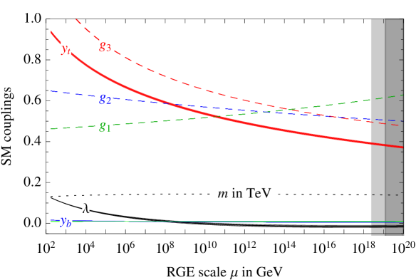
Figure 1: Renormalisation of the SM gauge couplings g1=5/3gY,g2,g3subscript𝑔153subscript𝑔𝑌subscript𝑔2subscript𝑔3g_{1}=\sqrt{5/3}g_{Y},g_{2},~{}g_{3}, of the top, bottom and τ𝜏\tau couplings (ytsubscript𝑦𝑡y_{t}, ybsubscript𝑦𝑏y_{b}, yτsubscript𝑦𝜏y_{\tau}), of the Higgs quartic coupling λ𝜆\lambda and of the Higgs mass parameter m𝑚m. All parameters are defined in the ms¯¯ms\overline{\mbox{\sc ms}} scheme. We include two-loop thresholds at the weak scale and three-loop RG equations. The thickness indicates the ±1σplus-or-minus1𝜎\pm 1\sigma uncertainties in Mt,Mh,α3subscript𝑀𝑡subscript𝑀subscript𝛼3M_{t},M_{h},\alpha_{3}.

4.1 SM couplings at the Planck scale

The first issue we want to address concerns the size of the SM coupling constants. When we try to extract information from the values of the coupling constants, it is reasonable to analyse their values not at the weak scale, but at some high-energy scale where we believe the SM matches onto some extended theory. So, using our NNLO results, we extrapolate the SM couplings from their weak-scale values (as determined in section 3) to higher energies.

The evolution of the SM couplings up to a large cut-off scale is shown in fig. 1. At the Planck mass, we find the following values of the SM parameters:

g1(MPl)=0.6154+0.0003 (MtGeV-173.34)-0.0006 MW- 80.384 GeV0.014 GeV\\g2(MPl)=0.5055\\g3(MPl)=0.4873+0.0002α3(MZ)0.11840.0007\\yt(MPl)=0.3825+0.0051(MtGeV173.34)0.0021α3(MZ)0.11840.0007\\λ(MPl)=0.01430.0066(MtGeV173.34)+\\+0.0018α3(MZ)0.11840.0007+0.0029(MhGeV125.15)\\m(MPl)=129.4GeV+1.6GeV(MhGeV125.15)+\\0.25GeV(MtGeV173.34)+0.05GeVα3(MZ)0.11840.0007(61)subscriptg1subscript(MPl)=0.6154+0.0003 (subscriptMtGeV-173.34)-0.0006 subscriptMW- 80.384 GeV0.014 GeV\\subscriptg2subscript(MPl)=0.5055\\subscript𝑔3subscript𝑀Pl0.48730.0002subscript𝛼3subscript𝑀𝑍0.11840.0007\\subscript𝑦𝑡subscript𝑀Pl0.38250.0051subscript𝑀𝑡GeV173.340.0021subscript𝛼3subscript𝑀𝑍0.11840.0007\\𝜆subscript𝑀Pl0.01430.0066subscript𝑀𝑡GeV173.34\\missing-subexpression0.0018subscript𝛼3subscript𝑀𝑍0.11840.00070.0029subscript𝑀GeV125.15\\𝑚subscript𝑀Pl129.4GeV1.6GeVsubscript𝑀GeV125.15\\missing-subexpression0.25GeVsubscript𝑀𝑡GeV173.340.05GeVsubscript𝛼3subscript𝑀𝑍0.11840.000761\halign to=0.0pt{\@eqnsel\hskip\@centering$\displaystyle{#}$&\global\@eqcnt\@ne\hskip 2\arraycolsep\hfil${#}$\hfil& \global\@eqcnt\tw@\hskip 2\arraycolsep$\displaystyle{#}$\hfil&\llap{#}\cr 0.0pt plus 1000.0pt$\displaystyle{g_{1}(M_{\rm Pl})&10.0pt\hfil${=&10.0pt$\displaystyle{0.6154+0.0003 \bigg{(}\frac{M_{t}}{\,{\rm GeV}}-173.34\bigg{)}-0.0006 \frac{M_{W} - 80.384\,{\rm GeV}}{0.014\,{\rm GeV}} \\ g_{2}(M_{\rm Pl})&\hbox to0.0pt{\hss=&0.5055\\g_{3}(M_{\rm Pl})&=&0.4873+0.0002\,\frac{\alpha_{3}(M_{Z})-0.1184}{0.0007}\\y_{t}(M_{\rm Pl})&=&0.3825+0.0051\bigg{(}\frac{M_{t}}{\,{\rm GeV}}-173.34\bigg{)}-0.0021\,\frac{\alpha_{3}(M_{Z})-0.1184}{0.0007}\\\lambda(M_{\rm Pl})&=&-0.0143-0.0066\bigg{(}\frac{M_{t}}{\,{\rm GeV}}-173.34\bigg{)}+\\&&+0.0018\,\frac{\alpha_{3}(M_{Z})-0.1184}{0.0007}+0.0029\bigg{(}\frac{M_{h}}{\,{\rm GeV}}-125.15\bigg{)}\\m(M_{\rm Pl})&=&129.4\,{\rm GeV}+1.6\,{\rm GeV}\bigg{(}\frac{M_{h}}{\,{\rm GeV}}-125.15\bigg{)}+\\&&-0.25\,{\rm GeV}\bigg{(}\frac{M_{t}}{\,{\rm GeV}}-173.34\bigg{)}+0.05\,{\rm GeV}\,\frac{\alpha_{3}(M_{Z})-0.1184}{0.0007}&(61)\cr}}}}}

All Yukawa couplings, other than the one of the top quark, are very small. This is the well-known flavour problem of the SM, which will not be investigated in this paper.

The three gauge couplings and the top Yukawa coupling remain perturbative and are fairly weak at high energy, becoming roughly equal in the vicinity of the Planck mass. The near equality of the gauge couplings may be viewed as an indicator of an underlying grand unification even within the simple SM, once we allow for threshold corrections of the order of 10% around a scale of about 1016superscript101610^{16} GeV (of course, in the spirit of this paper, we are disregarding the acute naturalness problem). It is amusing to note that the ordering of the coupling constants at low energy is completely overturned at high energy. The (properly normalised) hypercharge coupling g1subscript𝑔1g_{1} becomes the largest coupling in the SM already at scales of about 1014superscript101410^{14} GeV, and the weak coupling g2subscript𝑔2g_{2} overcomes the strong coupling at about 1016superscript101610^{16} GeV. The top Yukawa becomes smaller than any of the gauge couplings at scales larger than about 1010superscript101010^{10} GeV.

Refer to caption      Refer to caption
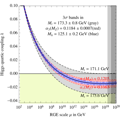
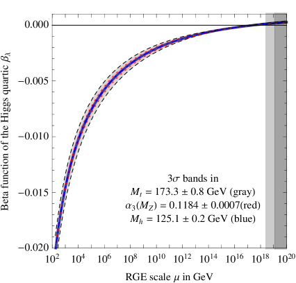
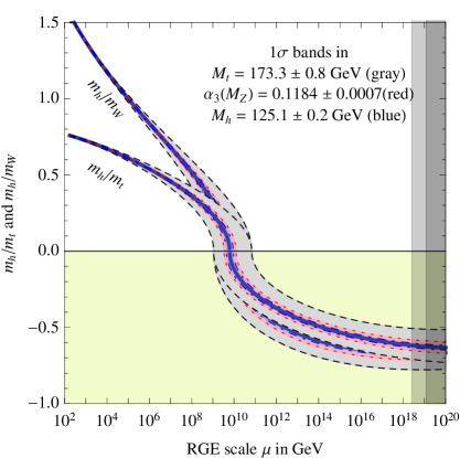
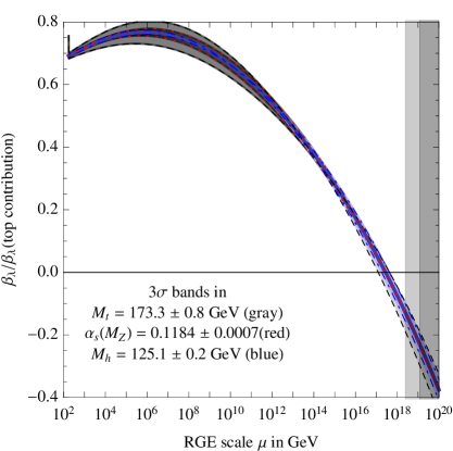
Figure 2: Upper: RG evolution of λ𝜆\lambda (left) and of βλsubscript𝛽𝜆\beta_{\lambda} (right) varying Mtsubscript𝑀𝑡M_{t}, α3(MZ)subscript𝛼3subscript𝑀𝑍\alpha_{3}(M_{Z}), Mhsubscript𝑀M_{h} by ±3σplus-or-minus3𝜎\pm 3\sigma. Lower: Same as above, with more “physical” normalisations. The Higgs quartic coupling is compared with the top Yukawa and weak gauge coupling through the ratios sign(λ)4|λ|/ytsign𝜆4𝜆subscript𝑦𝑡{\rm sign}(\lambda)\sqrt{4|\lambda|}/y_{t} and sign(λ)8|λ|/g2sign𝜆8𝜆subscript𝑔2{\rm sign}(\lambda)\sqrt{8|\lambda|}/g_{2}, which correspond to the ratios of running masses mh/mtsubscript𝑚subscript𝑚𝑡m_{h}/m_{t} and mh/mWsubscript𝑚subscript𝑚𝑊m_{h}/m_{W}, respectively (left). The Higgs quartic β𝛽\beta-function is shown in units of its top contribution, βλsubscript𝛽𝜆\beta_{\lambda}(top contribution) =3yt4/8π2absent3superscriptsubscript𝑦𝑡48superscript𝜋2=-3y_{t}^{4}/8\pi^{2} (right). The grey shadings cover values of the RG scale above the Planck mass MPl1.2×1019GeVsubscript𝑀Pl1.2superscript1019GeVM_{\rm Pl}\approx 1.2\times 10^{19}\,{\rm GeV}, and above the reduced Planck mass M¯Pl=MPl/8πsubscript¯𝑀Plsubscript𝑀Pl8𝜋\bar{M}_{\rm Pl}=M_{\rm Pl}/\sqrt{8\pi}.

The Higgs quartic coupling remains weak in the entire energy domain below MPlsubscript𝑀PlM_{\rm Pl}. It decreases with energy crossing λ=0𝜆0\lambda=0 at a scale of about 1010superscript101010^{10} GeV, see fig. 2 (upper left). Indeed, λ𝜆\lambda is the only SM coupling that is allowed to change sign during the RG evolution because it is not multiplicatively renormalised. For all other SM couplings, the β𝛽\beta functions are proportional to their respective couplings and crossing zero is not possible. This corresponds to the fact that λ=0𝜆0\lambda=0 is not a point of enhanced symmetry.

In fig. 2 (lower left) we compare the size of λ𝜆\lambda with the top Yukawa coupling ytsubscript𝑦𝑡y_{t} and the gauge coupling g2subscript𝑔2g_{2}, choosing a normalisation such that each coupling is equal to the corresponding particle mass, up to the same proportionality constant. In other words, we are plotting the ratios

sign(λ)×4|λ|/yt and sign(λ)×8|λ|/g2,sign(λ)×4|λ|/yt and sign(λ)×8|λ|/g2\hbox{${\rm sign}(\lambda)\times\sqrt{4|\lambda|}/y_{t}\qquad$ and $\qquad{\rm sign}(\lambda)\times\sqrt{8|\lambda|}/g_{2}$}\ , (62)

equal to the ratios of running masses mh/mtsubscript𝑚subscript𝑚𝑡m_{h}/m_{t} and mh/mWsubscript𝑚subscript𝑚𝑊m_{h}/m_{W}, respectively. Except for the region in which λ𝜆\lambda vanishes, the Higgs quartic coupling looks fairly “normal” with respect to the other SM couplings. Nonetheless, the RG effect reduces significantly the overall size of λ𝜆\lambda in its evolution from low to high energy. Although the central values of Higgs and top masses do not favour a scenario with vanishing Higgs self coupling at the Planck scale (MPlsubscript𝑀PlM_{\rm Pl}) — a possibility originally proposed in ref. [106, 107] and discussed more recently in ref. [108, 109, 110, 111, 4] — the smallness of λ𝜆\lambda around MPlsubscript𝑀PlM_{\rm Pl} offers reasons for speculation, as we will discuss later.

Another important feature of the RG evolution of λ𝜆\lambda is the slowing down of the running at high energy. As shown in fig. 2 (upper right), the corresponding Higgs quartic β𝛽\beta-function vanishes at a scale of about 1017superscript101710^{17}1018superscript101810^{18} GeV. In order to quantify the degree of cancellation in the β𝛽\beta-function, we plot in fig. 2 (lower right) βλsubscript𝛽𝜆\beta_{\lambda} in units of its pure top contribution. The vanishing of βλsubscript𝛽𝜆\beta_{\lambda} looks more like an accidental cancellation between various large contributions, rather than an asymptotic approach to zero. Given that the β𝛽\beta-functions of the other SM couplings are all different than zero, it is not evident to find valid symmetry or dynamical reasons for the vanishing of βλsubscript𝛽𝜆\beta_{\lambda} alone near MPlsubscript𝑀PlM_{\rm Pl}. However, the smallness of βλsubscript𝛽𝜆\beta_{\lambda} (and λ𝜆\lambda) at high energy implies that tiny variations of the input values of the couplings at MPlsubscript𝑀PlM_{\rm Pl} lead to wide fluctuations of the instability scale, thus justifying our refined calculation.
Refer to caption      Refer to caption
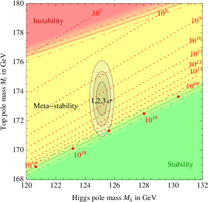
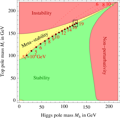
Figure 3: Left: SM phase diagram in terms of Higgs and top pole masses. The plane is divided into regions of absolute stability, meta-stability, instability of the SM vacuum, and non-perturbativity of the Higgs quartic coupling. The top Yukawa coupling becomes non-perturbative for Mt>230GeVsubscript𝑀𝑡230GeVM_{t}>230\,\,{\rm GeV}. The dotted contour-lines show the instability scale ΛIsubscriptΛ𝐼\Lambda_{I} in GeVGeV\,{\rm GeV} assuming α3(MZ)=0.1184subscript𝛼3subscript𝑀𝑍0.1184\alpha_{3}(M_{Z})=0.1184. Right: Zoom in the region of the preferred experimental range of Mhsubscript𝑀M_{h} and Mtsubscript𝑀𝑡M_{t} (the grey areas denote the allowed region at 1, 2, and 3σ𝜎\sigma). The three boundary lines correspond to 1-σ𝜎\sigma variations of α3(MZ)=0.1184±0.0007subscript𝛼3subscript𝑀𝑍plus-or-minus0.11840.0007\alpha_{3}(M_{Z})=0.1184\pm 0.0007, and the grading of the colours indicates the size of the theoretical error.

4.2 Derivation of the stability bound

In order to compute the stability bound on the Higgs mass one has to study the full effective potential and identify the critical Higgs field above which the potential becomes smaller than the value at the EW vacuum. We will refer to such critical energy as the instability scale ΛIsubscriptΛ𝐼\Lambda_{I}.

A first estimate of the instability scale can be obtained by approximating the effective potential with its RG-improved tree level expression. The analysis shows that the instability scale occurs at energies much bigger than the EW scale. Thus, for our purposes, the approximation of neglecting v𝑣v with respect to the value of the field hh is amply justified. Under this assumption, the effective potential (in the relevant region hvmuch-greater-than𝑣h\gg v) becomes

Veff(h)=λeff(h)h44.subscript𝑉effsubscript𝜆effsuperscript44V_{\rm eff}(h)=\lambda_{\rm eff}(h)\frac{h^{4}}{4}. (63)

The quantity λeffsubscript𝜆eff\lambda_{\rm eff} can be extracted from the effective potential at two loops [112] and is explicitly given in appendix C.

4.3 The SM phase diagram in terms of Higgs and top masses

The two most important parameters that determine the various EW phases of the SM are the Higgs and top-quark masses. In fig. 3 we update the phase diagram given in ref. [4] with our improved calculation of the evolution of the Higgs quartic coupling. The regions of stability, metastability, and instability of the EW vacuum are shown both for a broad range of Mhsubscript𝑀M_{h} and Mtsubscript𝑀𝑡M_{t}, and after zooming into the region corresponding to the measured values. The uncertainty from α3subscript𝛼3\alpha_{3} and from theoretical errors are indicated by the dashed lines and the colour shading along the borders. Also shown are contour lines of the instability scale ΛIsubscriptΛ𝐼\Lambda_{I}.

As previously noticed in ref. [4], the measured values of Mhsubscript𝑀M_{h} and Mtsubscript𝑀𝑡M_{t} appear to be rather special, in the sense that they place the SM vacuum in a near-critical condition, at the border between stability and metastability. In the neighbourhood of the measured values of Mhsubscript𝑀M_{h} and Mtsubscript𝑀𝑡M_{t}, the stability condition is well approximated by

Mh>129.6GeV+2.0(Mt173.34GeV)0.5GeVα3(MZ)0.11840.0007±0.3GeV.subscript𝑀plus-or-minus129.6GeV2.0subscript𝑀𝑡173.34GeV0.5GeVsubscript𝛼3subscript𝑀𝑍0.11840.00070.3GeVM_{h}>129.6\,{\rm GeV}+2.0(M_{t}-173.34\,{\rm GeV})-0.5\,{\rm GeV}\,\frac{\alpha_{3}(M_{Z})-0.1184}{0.0007}\pm 0.3\,{\rm GeV}\ . (64)

The quoted uncertainty comes only from higher order perturbative corrections. Other non-perturbative uncertainties associated with the relation between the measured value of the top mass and the actual definition of the top pole mass used here (presumably of the order of ΛQCDsubscriptΛQCD\Lambda_{\rm QCD}) are buried inside the parameter Mtsubscript𝑀𝑡M_{t} in eq. (64). For this reason we include a theoretical error in the top pole mass and take Mt=(173.34±0.76exp±0.3th)GeVsubscript𝑀𝑡plus-or-minus173.34subscript0.76expsubscript0.3thGeVM_{t}=(173.34\pm 0.76_{\rm exp}\pm 0.3_{\rm th})\,{\rm GeV}. Combining in quadrature theoretical uncertainties with experimental errors, we find

Mh>(129.6±1.5)GeV(stabilitycondition).subscript𝑀plus-or-minus129.61.5GeVstabilityconditionM_{h}>(129.6\pm 1.5)\,{\rm GeV}\qquad{\rm(stability~{}condition).} (65)

From this result we conclude that vacuum stability of the SM up to the Planck scale is excluded at 2.8σ2.8𝜎2.8\sigma (99.8% C.L. one-sided). Since the main source of uncertainty in eq. (64) comes from Mtsubscript𝑀𝑡M_{t}, any refinement in the measurement of the top mass is of great importance for the question of EW vacuum stability.

Since the experimental error on the Higgs mass is already fairly small and will be further reduced by future LHC analyses, it is becoming more appropriate to express the stability condition in terms of the pole top mass. We can express the stability condition of eq. (64) as

Mt<(171.53±0.15±0.23α3±0.15Mh)GeV=(171.53±0.42)GeV.subscript𝑀𝑡plus-or-minus171.530.15subscript0.23subscript𝛼3subscript0.15subscript𝑀GeVplus-or-minus171.530.42GeVM_{t}<(171.53\pm 0.15\pm 0.23_{\alpha_{3}}\pm 0.15_{M_{h}})\,{\rm GeV}=(171.53\pm 0.42)\,{\rm GeV}. (66)

In the latter equation we combined in quadrature the theoretical uncertainty with the experimental uncertainties on Mhsubscript𝑀M_{h} and α3subscript𝛼3\alpha_{3}.

Notice that the stability bound is scheme and gauge independent. While intermediate steps of the computation (threshold corrections, higher-order RG equations, and the effective potential) are scheme-dependent, the values of the effective potential at its local minima are scheme-independent physical observables, and thus the stability condition has the same property.

The instability scale ΛVsubscriptΛ𝑉\Lambda_{V} can be defined in a gauge-independent and scheme-independent way as ΛV(maxhVeff(h))1/4subscriptΛ𝑉superscriptsubscriptsubscript𝑉eff14\Lambda_{V}\equiv(\max_{h}V_{\rm eff}(h))^{1/4}, in terms of the value of the effective SM potential of eq. (63) at the maximum of its barrier. Numerically we find

log10ΛVGeV=9.5+0.7(MhGeV125.15)1.0(MtGeV173.34)+0.3α3(MZ)0.11840.0007.subscript10subscriptΛ𝑉GeV9.50.7subscript𝑀GeV125.151.0subscript𝑀𝑡GeV173.340.3subscript𝛼3subscript𝑀𝑍0.11840.0007\log_{10}\frac{\Lambda_{V}}{\,{\rm GeV}}=9.5+0.7\bigg{(}\frac{M_{h}}{\,{\rm GeV}}-125.15\bigg{)}-1.0\bigg{(}\frac{M_{t}}{\,{\rm GeV}}-173.34\bigg{)}+0.3\,\frac{\alpha_{3}(M_{Z})-0.1184}{0.0007}. (67)

The alternative definition of the instability scale, as the scale ΛλsubscriptΛ𝜆\Lambda_{\lambda} at which the running coupling λ𝜆\lambda vanishes, is scheme-dependent. In the ms¯¯ms\overline{\mbox{\sc ms}} scheme we find Λλ2ΛVsubscriptΛ𝜆2subscriptΛ𝑉\Lambda_{\lambda}\approx 2\Lambda_{V}. The alternative definition of the instability scale, as the scale ΛIsubscriptΛ𝐼\Lambda_{I} at which λeffsubscript𝜆eff\lambda_{\rm eff} vanishes, is gauge dependent. In the Landau gauge we find ΛI13ΛVsubscriptΛ𝐼13subscriptΛ𝑉\Lambda_{I}\approx 13\Lambda_{V} around the observed values of the SM parameters.
Refer to caption      Refer to caption

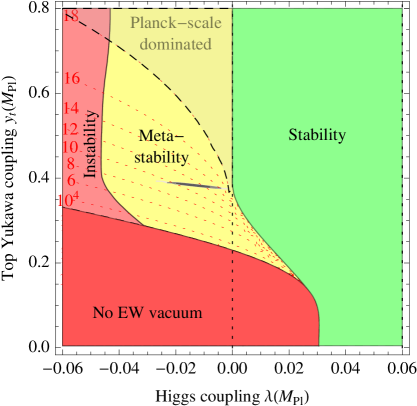
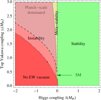
Figure 4: Left: SM phase diagram in terms of quartic Higgs coupling λ𝜆\lambda and top Yukawa coupling ytsubscript𝑦𝑡y_{t} renormalised at the Planck scale. The region where the instability scale ΛIsubscriptΛ𝐼\Lambda_{I} is larger than 1018GeVsuperscript1018GeV10^{18}\,\,{\rm GeV} is indicated as ‘Planck-scale dominated’. Right: Zoom around the experimentally measured values of the couplings, which correspond to the thin ellipse roughly at the centre of the panel. The dotted lines show contours of ΛIsubscriptΛ𝐼\Lambda_{I} in GeVGeV\,{\rm GeV}.

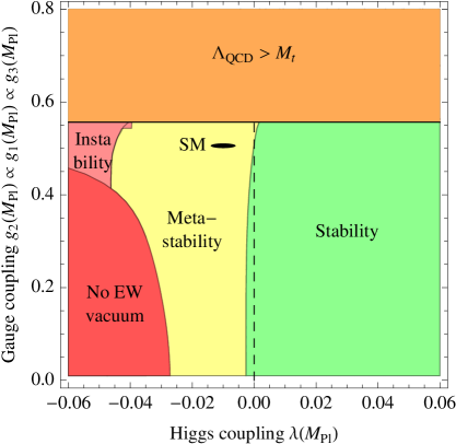
4.4 The SM phase diagram in terms of Planck-scale couplings

The discovery of the SM near-criticality has led to many theoretical speculations [27, 4, 28, 29, 30, 31, 32, 33, 34, 35, 36, 37, 38, 39, 40, 41, 42, 43, 44, 45, 46, 47, 48, 49, 50, 110, 111]. In order to address such speculations and to investigate if the measured value of Mhsubscript𝑀M_{h} is really special in the SM, it is more appropriate to study the phase diagram in terms of the Higgs quartic and the top Yukawa coupling evaluated at some high-energy scale, rather than at the weak scale. This is because of our theoretical bias that the SM is eventually embedded into a new framework at short distances, possibly as short as the Planck length. Therefore, it is more likely that information about the underlying theory is directly encoded in the high-energy coupling constants. For this reason in fig. 4 we recast the phase diagram of fig. 3 in terms of λ(MPl)𝜆subscript𝑀Pl\lambda(M_{\rm Pl}) and yt(MPl)subscript𝑦𝑡subscript𝑀Ply_{t}(M_{\rm Pl}). The diagram is shown in a broad range of couplings allowed by perturbativity, and also after zooming into the interesting region. The new area denoted as ‘no EW vacuum’ corresponds to a situation in which λ𝜆\lambda is negative at the weak scale, and therefore the usual Higgs vacuum does not exist. In the region denoted as ‘Planck-scale dominated’ the instability scale ΛIsubscriptΛ𝐼\Lambda_{I} is larger than 1018GeVsuperscript1018GeV10^{18}\,\,{\rm GeV}. In this situation we expect that both the Higgs potential and the tunnelling rate receive large gravitational corrections and any assessment about vacuum stability becomes unreliable.

From the left panel of fig. 4 it is evident that, even when we consider the situation in terms of high-energy couplings, our universe appears to live under very special conditions. The interesting theoretical question is to understand if the apparent peculiarity of λ(MPl)𝜆subscript𝑀Pl\lambda(M_{\rm Pl}) and yt(MPl)subscript𝑦𝑡subscript𝑀Ply_{t}(M_{\rm Pl}) carry any important information about phenomena well beyond the reach of any collider experiment. Of course this result could be just an accidental coincidence, because in reality the SM potential is significantly modified by new physics at low or intermediate scales. Indeed, the Higgs naturalness problem corroborates this possibility. However, both the reputed violation of naturalness in the cosmological constant and the present lack of new physics at the LHC cast doubts on the validity of the naturalness criterion for the Higgs boson. Of course, even without a natural EW sector, there are good reasons to believe in the existence of new degrees of freedom at intermediate energies. Neutrino masses, dark matter, axion, inflation, baryon asymmetry provide good motivations for the existence of new dynamics below the Planck mass. However, for each of these problems we can imagine solutions that either involve physics well above the instability scale or do not significantly modify the shape of the Higgs potential. As a typical example, take the see-saw mechanism. As shown in ref. [29], for neutrino masses smaller than 0.1 eV (as suggested by neutrino-oscillation data without mass degeneracies), either neutrino Yukawa couplings are too small to modify the running of λ𝜆\lambda or the right-handed neutrino masses are larger than the instability scale. In other words, a see-saw neutrino does not modify our conclusions about stability of the EW vacuum. Couplings of weak-scale dark matter to the Higgs boson are constrained to be small by WIMP direct searches (although dark-matter particles with weak interactions would modify the running of the weak gauge couplings, making the Higgs potential more stable).

Thus, it is not inconceivable that the special values of λ(MPl)𝜆subscript𝑀Pl\lambda(M_{\rm Pl}) and yt(MPl)subscript𝑦𝑡subscript𝑀Ply_{t}(M_{\rm Pl}) carry a significance and it is worth to investigate their consequences. In the next section we discuss several possible classes of solutions that explain the apparent peculiarity of the SM parameters.

Finally, we notice that extrapolating SM parameters above the Planck scale ignoring gravity (this is a questionable assumption) the hypercharge couplings hits a Landau pole at about 1042GeVsuperscript1042GeV10^{42}\,{\rm GeV}. Demanding perturbativity up to such scale (rather than up to the Planck scale), the bounds on the top and Higgs masses become stronger by about 10 and 20 GeV stronger respectively, and their measured values still lie in the region that can be extrapolated up to such high scale.

5 Interpretations of the high-energy SM couplings

The first possible interpretation, discussed in section 5.1, is the result of new dynamics occurring at some high-energy scale, the others find their most natural implementations in the multiverse.

5.1 Matching conditions

The special value of the Higgs quartic coupling could be the result of a matching condition with some high-energy theory in the vicinity of MPlsubscript𝑀PlM_{\rm Pl}. It is not difficult to imagine theories able to drive λ(MPl)𝜆subscript𝑀Pl\lambda(M_{\rm Pl}) to zero: high-scale supersymmetry with tanβ=1𝛽1\tan\beta=1 [113, 114, 115, 116, 117, 118]; partial N=2𝑁2N=2 supersymmetry insuring D𝐷D-flatness [119, 120]; an approximate Goldstone or shift symmetry [121, 122]; an infrared fixed-point of some transplanckian physics [111]; a power-law running in a quasi-conformal theory. Present data suggest that an exact zero of λ𝜆\lambda is reached at scales of about 1010superscript101010^{10}1012superscript101210^{12} GeV, see eq (67), well below the Planck mass. It is not difficult to imagine theories that give λ(MPl)𝜆subscript𝑀Pl\lambda(M_{\rm Pl}) in agreement with eq. (4.1) as a result of a vanishing matching condition modified by threshold corrections.

Supersymmetry is probably one of the best candidates able to explain the vanishing of λ𝜆\lambda as a high-energy boundary condition, because of the natural appearance of radiatively-stable flat directions. Such flat directions give a well-grounded justification for scalar particles with vanishing potentials, and yet interacting at zero momentum (contrary to the case of Goldstone bosons).

Note also that the smallness of the Higgs quartic β𝛽\beta-function at high energy is the key ingredient that allows for the possibility of extending the SM up to a matching scale much larger than ΛIsubscriptΛ𝐼\Lambda_{I}. If λ𝜆\lambda ran fast above ΛIsubscriptΛ𝐼\Lambda_{I}, it would rapidly trigger vacuum instability and the region of metastability would be limited to SM cut-off scales only slightly larger than ΛIsubscriptΛ𝐼\Lambda_{I}. This is another peculiarity of the measured values of Mhsubscript𝑀M_{h} and Mtsubscript𝑀𝑡M_{t}.

5.2 Criticality as an attractor

Statistical properties of the multiverse offer alternatives to dynamical determinations of λ(MPl)𝜆subscript𝑀Pl\lambda(M_{\rm Pl}) from matching conditions with new theories. The first possibility we consider is motivated by the observation that the measured value of Mhsubscript𝑀M_{h} looks special, in the sense that it corresponds to a near-critical parameter separating two phases. As remarked in ref. [123], also Higgs naturalness can be viewed as a problem of near-criticality between two phases (i.e. why is the Higgs bilinear carefully selected just to place our universe at the edge between the broken and unbroken EW phases?). This leads to the speculation that, within the multiverse, critical points are attractors. If this vision is correct, the probability density in the multiverse is peaked around the boundaries between different phases, and generic universes are likely to live near critical lines. Then, near-criticality would be the result of probability distributions in the multiverse, and would not necessarily follow from anthropic considerations. In this picture, the Higgs parameters found in our universe are not at all special. On the contrary, they correspond to the most likely occurrence in the multiverse.

There are many natural phenomena in which near-criticality emerges as an attractor [124]. A typical example is given by the slope angle of sand dunes. While one could expect to find in a beach sand dunes with any possible slope angles, in practice the vast majority of dunes have a slope angle roughly equal to the so-called “angle of repose”. The angle of repose is the steepest angle of descent, which is achieved when the material forming the pile is at a critical condition on the verge of sliding. The angle of repose depends on size and shape of the material granularity, and for sand is usually about 30–35 degrees. The typicality of finding sand dunes with slope angles near the critical value is simply understood in terms of the forces that shape dunes. Wind builds up the dune moving sand up to the top; gravity makes the pile collapse under its own weight when the dune is too steep. As a result, near-criticality is the most likely condition, as a compromise between two competing effects.

Something similar could happen with the Higgs parameters in the multiverse. Suppose that the probability distribution of the Higgs quartic coupling in the multiverse is not uniform, but is a monotonically decreasing function of λ𝜆\lambda. In other words, there is a pressure in the multiverse towards the smallest (possibly negative) λ𝜆\lambda. However, in universes where λ𝜆\lambda is sufficiently negative, the Higgs field is destabilised, forming a bubble of AdS space with a negative cosmological constant of order MPl4superscriptsubscript𝑀Pl4-M_{\rm Pl}^{4} in its interior. Such regions of space would rapidly contract and finally disappear. Therefore, the cosmological evolution removes regions that correspond to unstable EW vacua, leaving the vast majority of universes crowded around the critical boundary. It is amusing to note the strict analogy with the case of sand dunes. The “wind” of the multiverse pushes the Higgs quartic coupling towards smaller values until space collapses under the effect of AdS gravity. As a result, the typical Higgs quartic coupling lies around the critical value.

We can also imagine alternative scenarios. Suppose that the Higgs quartic coupling is a function of some new fields ΦΦ\Phi participating in Planckian dynamics and that their vacuum structure prefers low values of λ𝜆\lambda, as before. Once λ𝜆\lambda becomes smaller than the critical value, the Higgs potential develops an instability at large field values. If tunnelling is sufficiently fast, the Higgs field slides towards Planckian scales. Such large Higgs configurations will in general affect the scalar potential of the fields ΦΦ\Phi, which will readjust into a different vacuum structure. The new vacua will give a different probability distribution for the Higgs quartic coupling λ𝜆\lambda and it is imaginable that now larger values of λ𝜆\lambda are preferred. In summary: universes in the stable or metastable phases will experience pressure towards small λ𝜆\lambda; universes in the unstable phase will experience pressure towards large λ𝜆\lambda. As a result, the most probable universes lie around the critical line separating the two phases.

We stress that these examples do not use anthropic arguments: near-criticality is achieved by cosmological selection and/or by probability distributions in the multiverse. Nevertheless, the proximity of our universe to an inhospitable phase, as shown in fig. 4, could be viewed as an indication that the principle of ‘living dangerously’ is at work, in a way similar to the case of the cosmological constant [125]. One can assume, as before, that the probability distribution function of λ(MPl)𝜆subscript𝑀Pl\lambda(M_{\rm Pl}) in the multiverse is skewed towards the lowest possible values, making it more likely for our universe to live in the leftmost region of fig. 4. The anthropic boundary of EW instability limits the allowed parameter space, giving a justification of why our universe is ‘living dangerously’, with conditions for stability barely satisfied.

5.3 Double criticality of Higgs and top couplings

From fig. 4 we can infer more than just criticality of the Higgs quartic coupling. Indeed, this figure shows that the measured values of the Higgs and top masses lie in the region corresponding not only to the lowest possible values of λ(MPl)𝜆subscript𝑀Pl\lambda(M_{\rm Pl}) allowed by (meta)stability, but also to the smallest possible value of yt(MPl)subscript𝑦𝑡subscript𝑀Ply_{t}(M_{\rm Pl}), once λ(MPl)𝜆subscript𝑀Pl\lambda(M_{\rm Pl}) has been selected. Indeed, for small Higgs quartic (λ(MPl)<0.02𝜆subscript𝑀Pl0.02\lambda(M_{\rm Pl})<0.02), there is a non-vanishing minimum value of yt(MPl)subscript𝑦𝑡subscript𝑀Ply_{t}(M_{\rm Pl}) required to avoid instability.

This special feature is related to the approximate vanishing of βλsubscript𝛽𝜆\beta_{\lambda} around the Planck mass. Indeed, for fixed λ(MPl)𝜆subscript𝑀Pl\lambda(M_{\rm Pl}), the top Yukawa coupling has the effect to stabilise the potential, as we evolve from high to low energies. Without a sizeable contribution from ytsubscript𝑦𝑡y_{t}, the gauge couplings tend to push λ𝜆\lambda towards more smaller (and eventually negative) values, leading to an instability. Therefore, whenever λ(MPl)𝜆subscript𝑀Pl\lambda(M_{\rm Pl}) is small or negative, a non-zero yt(MPl)subscript𝑦𝑡subscript𝑀Ply_{t}(M_{\rm Pl}) is necessary to compensate the destabilising effect of gauge couplings. These considerations assume that λ(MPl)𝜆subscript𝑀Pl\lambda(M_{\rm Pl}) and yt(MPl)subscript𝑦𝑡subscript𝑀Ply_{t}(M_{\rm Pl}) scan widely in the multiverse, while gauge couplings do not. The case of scanning gauge couplings will be discussed in section 6.1.

It is a remarkable coincidence that the measured values of the Higgs and top masses correspond rather precisely to the simultaneous minima of both λ(MPl)𝜆subscript𝑀Pl\lambda(M_{\rm Pl}) and yt(MPl)subscript𝑦𝑡subscript𝑀Ply_{t}(M_{\rm Pl}). In other words, it is curious that not only do we live in the narrow vertical yellow stripe of fig. 4 — the minimum of λ(MPl)𝜆subscript𝑀Pl\lambda(M_{\rm Pl}) — but also near the bottom of the funnel – the minimum of yt(MPl)subscript𝑦𝑡subscript𝑀Ply_{t}(M_{\rm Pl}). Near-criticality holds for both the Higgs quartic and the top Yukawa coupling. Our universe is doubly enjoying a ‘dangerous life’ with respect to EW stability.

5.4 Statistics

We can also envisage a different situation within the multiverse hypothesis, namely that λ(MPl)𝜆subscript𝑀Pl\lambda(M_{\rm Pl}) and yt(MPl)subscript𝑦𝑡subscript𝑀Ply_{t}(M_{\rm Pl}) are determined statistically, while neither criticality nor anthropic arguments play any role. To illustrate this possibility we argue that some of the features of the high-energy SM couplings described in section 4.1 can be explained, at a purely qualitative level, by the existence of a multiverse in which SM coupling constants scan. We will not try to address the hierarchies in the Yukawa couplings. These could emerge as the result of an underlying flavour symmetry, remnant of a sector external to the SM, although it is not excluded that the pattern of Yukawa couplings is the result of the statistical properties of the multiverse [126, 127, 128, 129]. Here we keep an agnostic point of view on the issue of flavour and concentrate only on Higgs quartic, top-Yukawa, and gauge couplings.

In order to describe the multiverse, we introduce some new scalar fields ΦisubscriptΦ𝑖\Phi_{i} (i=1,,N𝑖1𝑁i=1,\dots,N), each having p𝑝p different vacuum configurations. The total number of possible vacua is pNsuperscript𝑝𝑁p^{N}, which is huge for large N𝑁N. If this multiverse of vacua is a viable candidate to solve the cosmological constant problem (i.e. to explain why somewhere in the multiverse the cosmological constant could be 10120superscript1012010^{120} times smaller than MPl4superscriptsubscript𝑀Pl4M_{\rm Pl}^{4}), then it is reasonable that pNsuperscript𝑝𝑁p^{N} should be at least 10120superscript1012010^{120}. So we envisage a situation in which N𝑁N is at least 𝒪(102)𝒪superscript102{\cal O}(10^{2}), which is not inconceivable in a string framework.

To describe the scanning of the SM couplings within this multiverse, we assume that the SM fields are coupled to the fields ΦΦ\Phi in the most general way,

=ZG(Φ)4FμνFμν+ZH(Φ)|DμH|2+(iZψ(Φ)ψ¯D/ψ+Yab(Φ)ψ¯aHψb+h.c.)Λ(Φ)|H|4.\mathscr{L}=-\frac{Z_{G}(\Phi)}{4}F_{\mu\nu}F^{\mu\nu}+Z_{H}(\Phi)\left|D_{\mu}H\right|^{2}+\left(iZ_{\psi}(\Phi)\bar{\psi}{D\!\!\!\!/\,}\psi+Y_{ab}(\Phi)\bar{\psi}_{a}H\psi_{b}+{\rm h.c.}\right)-\Lambda(\Phi)|H|^{4}. (68)

Here Fμνsubscript𝐹𝜇𝜈F_{\mu\nu} and ψ𝜓\psi collectively denote the SM gauge and fermion fields, and H𝐻H is the Higgs doublet. The physical SM coupling constants are given by

g=ZG1/2,yt=ZtL1/2YtZH1/2ZtR1/2,λ=ZH2Λ,formulae-sequence𝑔superscriptsubscript𝑍𝐺12formulae-sequencesubscript𝑦𝑡superscriptsubscript𝑍subscript𝑡𝐿12subscript𝑌𝑡superscriptsubscript𝑍𝐻12superscriptsubscript𝑍subscript𝑡𝑅12𝜆superscriptsubscript𝑍𝐻2Λg=Z_{G}^{-1/2},~{}~{}~{}y_{t}=Z_{t_{L}}^{-1/2}Y_{t}Z_{H}^{-1/2}Z_{t_{R}}^{-1/2},~{}~{}~{}\lambda=Z_{H}^{-2}\Lambda~{}, (69)

where the functions ZG,ψ,Hsubscript𝑍𝐺𝜓𝐻Z_{G,\psi,H}, Y𝑌Y, and ΛΛ\Lambda are evaluated at a vacuum of the fields ΦΦ\Phi. Since the fields ΦΦ\Phi have pNsuperscript𝑝𝑁p^{N} vacua, the SM couplings effectively scan in this multiverse. The coupling constants in eq. (69) are evaluated at the high-energy scale, here identified with MPlsubscript𝑀PlM_{\rm Pl}, where the new dynamics is integrated out.

For simplicity, we consider the toy example of multiverse proposed in ref. [130], in which each field ΦisubscriptΦ𝑖\Phi_{i} has two vacua (p=2𝑝2p=2) called Φi(+)superscriptsubscriptΦ𝑖\Phi_{i}^{(+)} and Φi()superscriptsubscriptΦ𝑖\Phi_{i}^{(-)}. We also assume that each of the functions ZG,ψ,Hsubscript𝑍𝐺𝜓𝐻Z_{G,\psi,H}, Y𝑌Y, ΛΛ\Lambda (let us call them collectively Z𝑍Z, to simplify notation) can be split as a sum of the contributions of the different fields ΦisubscriptΦ𝑖\Phi_{i},

Z(Φ1,,Φn)=i=1NZi(Φi),Z={ZG,Zψ,ZH,Y,Λ}.formulae-sequence𝑍subscriptΦ1subscriptΦ𝑛superscriptsubscript𝑖1𝑁subscript𝑍𝑖subscriptΦ𝑖𝑍subscript𝑍𝐺subscript𝑍𝜓subscript𝑍𝐻𝑌ΛZ(\Phi_{1},\dots,\Phi_{n})=\sum_{i=1}^{N}Z_{i}(\Phi_{i}),~{}~{}~{}~{}~{}~{}~{}~{}Z=\{Z_{G},Z_{\psi},Z_{H},Y,\Lambda\}. (70)

This is a consistent hypothesis, as long as the fields ΦΦ\Phi are mutually weakly-interacting. In this case, any mixed interaction is generated only by small loop effects and can be ignored. Under this hypothesis, the 2Nsuperscript2𝑁2^{N} values of Z𝑍Z corresponding to the vacua of ΦΦ\Phi can written as

Z=i=1N(Zi(S)+ηiZi(D)),Zi(S)=Zi(Φi(+))+Zi(Φi())2,Zi(D)=Zi(Φi(+))Zi(Φi())2,formulae-sequence𝑍superscriptsubscript𝑖1𝑁superscriptsubscript𝑍𝑖𝑆subscript𝜂𝑖superscriptsubscript𝑍𝑖𝐷formulae-sequencesuperscriptsubscript𝑍𝑖𝑆subscript𝑍𝑖superscriptsubscriptΦ𝑖subscript𝑍𝑖superscriptsubscriptΦ𝑖2superscriptsubscript𝑍𝑖𝐷subscript𝑍𝑖superscriptsubscriptΦ𝑖subscript𝑍𝑖superscriptsubscriptΦ𝑖2Z=\sum_{i=1}^{N}\left(Z_{i}^{(S)}+\eta_{i}Z_{i}^{(D)}\right),~{}~{}~{}Z_{i}^{(S)}=\frac{Z_{i}(\Phi_{i}^{(+)})+Z_{i}(\Phi_{i}^{(-)})}{2},~{}~{}~{}Z_{i}^{(D)}=\frac{Z_{i}(\Phi_{i}^{(+)})-Z_{i}(\Phi_{i}^{(-)})}{2}, (71)

where ηi=±1subscript𝜂𝑖plus-or-minus1\eta_{i}=\pm 1. Each of the 2Nsuperscript2𝑁2^{N} vacua (and each of the 2Nsuperscript2𝑁2^{N} values of Z𝑍Z) is labeled by the vector η=(ηi,,ηN)𝜂subscript𝜂𝑖subscript𝜂𝑁\eta=(\eta_{i},\dots,\eta_{N}).

The normalised probability distribution of Z𝑍Z within the multiverse of vacua is given by

ρ(Z)=2Nηδ(ZNZ¯i=1NηiZi(D)),Z¯1Ni=1NZi(S).formulae-sequence𝜌𝑍superscript2𝑁subscript𝜂𝛿𝑍𝑁¯𝑍superscriptsubscript𝑖1𝑁subscript𝜂𝑖superscriptsubscript𝑍𝑖𝐷¯𝑍1𝑁superscriptsubscript𝑖1𝑁superscriptsubscript𝑍𝑖𝑆\rho(Z)=2^{-N}\sum_{\eta}\delta\left(Z-N\bar{Z}-\sum_{i=1}^{N}\eta_{i}Z_{i}^{(D)}\right),\qquad\bar{Z}\equiv\frac{1}{N}\sum_{i=1}^{N}Z_{i}^{(S)}. (72)

Using the central limit theorem, the discrete sum over the 2Nsuperscript2𝑁2^{N} configurations of η𝜂\eta in eq. (72) can be approximated for large N𝑁N with a Gaussian distribution [130]

ρ(Z)=12πNΔ2exp[(ZNZ¯)22NΔ2],Δ2=1Ni=1NZi(D)2.formulae-sequence𝜌𝑍12𝜋𝑁superscriptΔ2superscript𝑍𝑁¯𝑍22𝑁superscriptΔ2superscriptΔ21𝑁superscriptsubscript𝑖1𝑁superscriptsuperscriptsubscript𝑍𝑖𝐷2\rho(Z)=\frac{1}{\sqrt{2\pi N\Delta^{2}}}\exp\left[-\frac{(Z-N\bar{Z})^{2}}{2N\Delta^{2}}\right],\qquad\Delta^{2}=\frac{1}{N}\sum_{i=1}^{N}{Z_{i}^{(D)}}^{2}. (73)

This shows that Z𝑍Z densely scans around NZ¯𝑁¯𝑍N\bar{Z} with an approximately flat distribution in the range |ZNZ¯|<NΔ𝑍𝑁¯𝑍𝑁Δ|Z-N\bar{Z}|<\sqrt{N}\Delta.

For generic couplings, we expect that Z¯¯𝑍\bar{Z} and ΔΔ\Delta are quantities of order unity, and thus Z𝑍Z is 𝒪(N)𝒪𝑁{\cal O}(N) with a relative uncertainty of order 1/N1𝑁1/\sqrt{N}. Plugging this result (which is valid for Z=ZG,ψ,H𝑍subscript𝑍𝐺𝜓𝐻Z=Z_{G,\psi,H}, Y𝑌Y, ΛΛ\Lambda) into eq. (69), we find

g,yt1N,λ1N.formulae-sequencesimilar-to𝑔subscript𝑦𝑡1𝑁similar-to𝜆1𝑁g,y_{t}\sim\frac{1}{\sqrt{N}},\qquad\lambda\sim\frac{1}{N}. (74)

For N100similar-to𝑁100N\sim 100, we obtain that gauge and top-Yukawa couplings are predicted to be 𝒪(101)𝒪superscript101{\cal O}(10^{-1}) at around MPlsubscript𝑀PlM_{\rm Pl}, while the Higgs quartic coupling is 𝒪(102)𝒪superscript102{\cal O}(10^{-2}), in good qualitative agreement with experimental data. Indeed, adopting a ‘physical’ normalisation of couplings as in fig. 2 (lower left), the SM predicts g1,2,3(MPl)/2yt(MPl)4|λ(MPl)|0.3subscript𝑔123subscript𝑀Pl2subscript𝑦𝑡subscript𝑀Pl4𝜆subscript𝑀Pl0.3g_{1,2,3}(M_{\rm Pl})/\sqrt{2}\approx y_{t}(M_{\rm Pl})\approx\sqrt{4|\lambda(M_{\rm Pl})|}\approx 0.3.

The different behaviour with N𝑁N in eq. (74) arises because λ𝜆\lambda is a quartic coupling, while g𝑔g and ytsubscript𝑦𝑡y_{t} are cubic couplings. Note that this framework suggests a hierarchy between g𝑔g, ytsubscript𝑦𝑡y_{t} on one side, and λ𝜆\lambda on the other side, but does not predict that λ𝜆\lambda should vanish at MPlsubscript𝑀PlM_{\rm Pl}, again as indicated by data. Actually, since λ𝜆\lambda scans by a relative amount 𝒪(1/N)𝒪1𝑁{\cal O}(1/\sqrt{N}), a vanishing value of λ(MPl)𝜆subscript𝑀Pl\lambda(M_{\rm Pl}) turns out to be fairly improbable in this setup.

6 More on SM phase diagrams
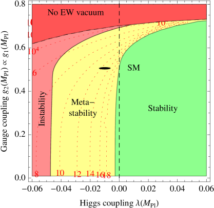
Refer to caption      Refer to caption
Figure 5: SM phase diagram in terms of the Higgs quartic coupling λ(MPl)𝜆subscript𝑀Pl\lambda(M_{\rm Pl}) and of the gauge coupling g2(MPl)subscript𝑔2subscript𝑀Plg_{2}(M_{\rm Pl}). Left: A common rescaling factor is applied to the electro-weak gauge couplings g1subscript𝑔1g_{1} and g2subscript𝑔2g_{2}, while g3subscript𝑔3g_{3} is kept constant. Right: A common rescaling factor is applied to all SM gauge couplings g1,g2,g3subscript𝑔1subscript𝑔2subscript𝑔3g_{1},g_{2},g_{3}, such that a 10%percent1010\% increase in the strong gauge coupling at the Planck scale makes ΛQCDsubscriptΛQCD\Lambda_{\rm QCD} larger than the weak scale. The measured values of the couplings correspond to the small ellipse marked as ‘SM’.

6.1 The SM phase diagram in terms of gauge couplings

So far we have been studying the phase diagram in terms of Higgs and top masses or couplings, keeping the other SM parameters fixed. This is reasonable, since the EW vacuum is mostly influenced by the Higgs and top quark. However, in the multiverse, other parameters can scan too and it is interesting to study how they affect our results.

We start by considering the scanning of weak couplings defined at some high-energy scale, which we identify with MPlsubscript𝑀PlM_{\rm Pl}. The impact of the gauge couplings g1subscript𝑔1g_{1} and g2subscript𝑔2g_{2} can be understood from the leading terms of the RG equation for the Higgs quartic coupling

(4π)2dλdlnμ¯2=3yt4+6yt2λ+12λ2+916(g24+25g22g12+325g14)92λ(g22+g125)+.superscript4𝜋2𝑑𝜆𝑑superscript¯𝜇23superscriptsubscript𝑦𝑡46superscriptsubscript𝑦𝑡2𝜆12superscript𝜆2916superscriptsubscript𝑔2425superscriptsubscript𝑔22superscriptsubscript𝑔12325superscriptsubscript𝑔1492𝜆superscriptsubscript𝑔22superscriptsubscript𝑔125(4\pi)^{2}\,\frac{d\lambda}{d\ln\bar{\mu}^{2}}=-3y_{t}^{4}+6y_{t}^{2}\lambda+12\lambda^{2}+\frac{9}{16}\left(g_{2}^{4}+\frac{2}{5}g_{2}^{2}g_{1}^{2}+\frac{3}{25}g_{1}^{4}\right)-\frac{9}{2}\lambda\left(g_{2}^{2}+\frac{g_{1}^{2}}{5}\right)+\cdots. (75)

For small λ(MPl)𝜆subscript𝑀Pl\lambda(M_{\rm Pl}), the weak gauge couplings have the effect of reducing even further the Higgs quartic coupling in its evolution towards lower energies, thus contributing to destabilise the potential. For large λ(MPl)𝜆subscript𝑀Pl\lambda(M_{\rm Pl}), they tend to make λ𝜆\lambda grow at lower energy.

We quantify the situation by plotting in fig. 5 (left) the SM phase diagram in terms of λ(MPl)𝜆subscript𝑀Pl\lambda(M_{\rm Pl}) and g2(MPl)subscript𝑔2subscript𝑀Plg_{2}(M_{\rm Pl}). For simplicity, we scan over the hypercharge coupling g1(MPl)subscript𝑔1subscript𝑀Plg_{1}(M_{\rm Pl}) by keeping fixed the ratio g1(MPl)/g2(MPl)=1.22subscript𝑔1subscript𝑀Plsubscript𝑔2subscript𝑀Pl1.22g_{1}(M_{\rm Pl})/g_{2}(M_{\rm Pl})=1.22 as in the SM, while yt(MPl)subscript𝑦𝑡subscript𝑀Ply_{t}(M_{\rm Pl}) and g3(MPl)subscript𝑔3subscript𝑀Plg_{3}(M_{\rm Pl}) are held to their SM values. As in previous cases, also the phase diagram in terms of weak gauge couplings shows the peculiar characteristic of the SM parameters to live close to the phase boundary. (Note that the figure is zoomed around the region of the physical values, so that the proximity to the boundary is not emphasised.)

Figure 5 (left) shows that the weak gauge couplings in the SM lie near the maximum possible values that do not lead to a premature decay of the EW vacuum. Were g2subscript𝑔2g_{2} and g1subscript𝑔1g_{1} 50% larger than their actual values, we wouldn’t be here speculating on the peculiarity of the Higgs mass.

Next, we discuss the impact of scanning the strong gauge coupling constant. In fig. 5 (right) we show the phase diagram in the plane λ(MPl)𝜆subscript𝑀Pl\lambda(M_{\rm Pl}), g2(MPl)subscript𝑔2subscript𝑀Plg_{2}(M_{\rm Pl}), obtained by varying all three gauge couplings by a common rescaling factor. The top Yukawa coupling yt(MPl)subscript𝑦𝑡subscript𝑀Ply_{t}(M_{\rm Pl}) is held fixed at its SM value and so, as the other couplings scan, the top mass does not correspond to the measured value.

The coupling g3subscript𝑔3g_{3} affects βλsubscript𝛽𝜆\beta_{\lambda} only at two loops, but it has a more important role in the RG evolution of the top Yukawa coupling, whose leading terms are given by

(4π)2dyt2dlnμ¯2=yt2(92yt28g3294g221720g12)+.superscript4𝜋2𝑑superscriptsubscript𝑦𝑡2𝑑superscript¯𝜇2superscriptsubscript𝑦𝑡292superscriptsubscript𝑦𝑡28superscriptsubscript𝑔3294superscriptsubscript𝑔221720superscriptsubscript𝑔12(4\pi)^{2}\,\frac{dy_{t}^{2}}{d\ln\bar{\mu}^{2}}=y_{t}^{2}\left(\frac{9}{2}y_{t}^{2}-8g_{3}^{2}-\frac{9}{4}g_{2}^{2}-\frac{17}{20}g_{1}^{2}\right)+\cdots. (76)

When the value of g3subscript𝑔3g_{3} is reduced at fixed yt(MPl)subscript𝑦𝑡subscript𝑀Ply_{t}(M_{\rm Pl}), the low-energy top Yukawa coupling becomes smaller. This reduces the stabilising effect of the top for a given λ(MPl)𝜆subscript𝑀Pl\lambda(M_{\rm Pl}) and explains the appearance in fig. 5 (right) at small gauge couplings of a ‘No EW vacuum’ region (where λ𝜆\lambda is negative at the weak scale).

On the other hand, when g3subscript𝑔3g_{3} is increased, the value of ΛQCDsubscriptΛQCD\Lambda_{\rm QCD} grows rapidly. Whenever

α3(MPl)>6π21ln(MPl/Mt),subscript𝛼3subscript𝑀Pl6𝜋21subscript𝑀Plsubscript𝑀𝑡\alpha_{3}(M_{\rm Pl})>\frac{6\pi}{21\ln(M_{\rm Pl}/M_{t})}, (77)

which corresponds to g3(MPl)>0.54subscript𝑔3subscript𝑀Pl0.54g_{3}(M_{\rm Pl})>0.54, the value of ΛQCDsubscriptΛQCD\Lambda_{\rm QCD} becomes larger than Mtsubscript𝑀𝑡M_{t}, preventing a perturbative extrapolation from the Planck to the weak scale. As shown in fig. 5 (right), this region is reached as soon as the SM gauge couplings are increased by only 11%. Once again, the SM gauge couplings live near the top of the range allowed by simple extrapolations of the minimal theory.
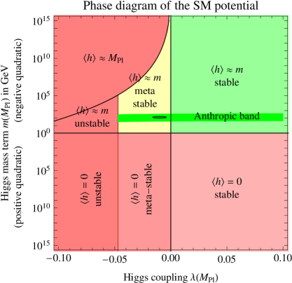
Refer to caption

Figure 6: Phase diagram of the SM in terms of the parameters of the Higgs potential evaluated at the Planck scale. In the metastability region, there is an upper bound on m𝑚m from the requirement of a Higgs vacuum at a finite field value. The green region is simple thanks to the fact that β(λ)=0𝛽𝜆0\beta(\lambda)=0 at MPlsubscript𝑀PlM_{\rm Pl}. On the vertical axis we plot |m(MPl)|𝑚subscript𝑀Pl|m(M_{\rm Pl})|, in the case of negative (above) and positive (below) Higgs quadratic term.

6.2 The SM phase diagram in terms of Higgs potential parameters

The Higgs mass parameter m𝑚m in the Higgs potential is the origin of the well-known naturalness problem. Here we show that the simple requirement of the existence of a non-trivial EW vacuum sets an upper bound on m𝑚m, which is completely independent of any naturalness argument.

Let us start by considering the tree-level Higgs potential in eq. (6). For m2>0superscript𝑚20m^{2}>0 and λ>0𝜆0\lambda>0, the potential has the usual non-trivial vacuum at h=v=m/2λdelimited-⟨⟩𝑣𝑚2𝜆\langle h\rangle=v=m/\sqrt{2\lambda}. However, since v𝑣v is proportional to m𝑚m and λ𝜆\lambda is negative above the instability scale ΛIsubscriptΛ𝐼\Lambda_{I}, the Higgs vacuum at finite field value no longer exists when m2superscript𝑚2m^{2} is too large. The upper bound on m2superscript𝑚2m^{2} can be estimated by considering the minimisation condition of the potential, including only the logarithmic running of λ𝜆\lambda, but neglecting the evolution of m𝑚m (which is a good approximation, as shown in fig. 1):

[2λ(v)+βλ(v)2]v2=m2.delimited-[]2𝜆𝑣subscript𝛽𝜆𝑣2superscript𝑣2superscript𝑚2\left[2\lambda(v)+\frac{\beta_{\lambda}(v)}{2}\right]v^{2}=m^{2}. (78)

For values of v𝑣v in the neighbourhood of ΛIsubscriptΛ𝐼\Lambda_{I}, we can approximate666In this analysis, we can safely neglect the non-logarithmic corrections to the effective potential and so we do not distinguish between λ𝜆\lambda and λeffsubscript𝜆eff\lambda_{\rm eff}. λ(v)βλ(ΛI)lnv/ΛI𝜆𝑣subscript𝛽𝜆subscriptΛ𝐼𝑣subscriptΛ𝐼\lambda(v)\approx\beta_{\lambda}(\Lambda_{I})\ln v/\Lambda_{I} and βλ(v)βλ(ΛI)subscript𝛽𝜆𝑣subscript𝛽𝜆subscriptΛ𝐼\beta_{\lambda}(v)\approx\beta_{\lambda}(\Lambda_{I}). Then we see that eq. (78) has a solution only if

m2<βλ(ΛI)e3/2ΛI2.superscript𝑚2subscript𝛽𝜆subscriptΛ𝐼superscript𝑒32superscriptsubscriptΛ𝐼2m^{2}<-\beta_{\lambda}(\Lambda_{I})\,e^{-3/2}\Lambda_{I}^{2}. (79)

Note that βλ(ΛI)subscript𝛽𝜆subscriptΛ𝐼\beta_{\lambda}(\Lambda_{I}) is negative in the SM.

Figure 6 shows the SM phase diagram in terms of the parameters λ(MPl)𝜆subscript𝑀Pl\lambda(M_{\rm Pl}) and m(MPl)𝑚subscript𝑀Plm(M_{\rm Pl}). The sign of each one of these parameters corresponds to different phases of the theory, such that λ(MPl)=m(MPl)=0𝜆subscript𝑀Pl𝑚subscript𝑀Pl0\lambda(M_{\rm Pl})=m(M_{\rm Pl})=0 is a tri-critical point.

The region denoted by ‘hMPldelimited-⟨⟩subscript𝑀Pl\langle h\rangle\approx M_{\rm Pl}’ corresponds to the case in which eq. (79) is not satisfied and there is no SM-like vacuum, while the Higgs field slides to large values. In the region of practical interest, the upper limit on m𝑚m is rather far from its actual physical value m=Mh𝑚subscript𝑀m=M_{h}, although it is much stronger than MPlsubscript𝑀PlM_{\rm Pl}, the ultimate ultraviolet cutoff of the SM. A much more stringent bound on m𝑚m can be derived from anthropic considerations [131] and the corresponding band in parameter space is shown in fig. 6. We find it remarkable that the simple request of the existence of a non-trivial Higgs vacuum, without any reference to naturalness considerations, gives a bound on the Higgs bilinear parameter m𝑚m. Unfortunately, for the physical value of λ𝜆\lambda, the actual numerical value of the upper bound is not of great practical importance.
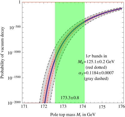
Refer to caption      Refer to caption
Figure 7: Left: The probability that electroweak vacuum decay happened in our past light-cone, taking into account the expansion of the universe. Right: The life-time of the electroweak vacuum, with two different assumptions for future cosmology: universes dominated by the cosmological constant (ΛΛ\LambdaCDM) or by dark matter (CDM).

6.3 Lifetime of the SM vacuum

The measured values of Mhsubscript𝑀M_{h} and Mtsubscript𝑀𝑡M_{t} indicate that the SM Higgs vacuum is not the true vacuum of the theory and that our universe is potentially unstable. The rate of quantum tunnelling out of the EW vacuum is given by the probability d/dVdt𝑑Weierstrass-p𝑑𝑉𝑑𝑡d\wp/dV\,dt of nucleating a bubble of true vacuum within a space volume dV𝑑𝑉dV and time interval dt𝑑𝑡dt [132, 133, 134]

d=dtdVΛB4eS(ΛB).𝑑Weierstrass-p𝑑𝑡𝑑𝑉superscriptsubscriptΛ𝐵4superscript𝑒𝑆subscriptΛ𝐵d\wp=dt\,dV~{}\Lambda_{B}^{4}\,e^{-S(\Lambda_{B})}\,. (80)

In eq. (80), S(ΛB)𝑆subscriptΛ𝐵S(\Lambda_{B}) is the action of the bounce of size R=ΛB1𝑅superscriptsubscriptΛ𝐵1R=\Lambda_{B}^{-1}, given by

S(ΛB)=8π23|λ(ΛB)|.𝑆subscriptΛ𝐵8superscript𝜋23𝜆subscriptΛ𝐵S(\Lambda_{B})=\frac{8\pi^{2}}{3|\lambda(\Lambda_{B})|}. (81)

At the classical level, the Higgs theory with only quartic coupling is scale-invariant and the size of the bounce ΛB1superscriptsubscriptΛ𝐵1\Lambda_{B}^{-1} is arbitrary. The RG flow breaks scale invariance and the tree level action gets replaced by the one-loop action, as calculated in ref. [24]. Then, ΛBsubscriptΛ𝐵\Lambda_{B} is determined as the scale at which ΛB4eS(ΛB)superscriptsubscriptΛ𝐵4superscript𝑒𝑆subscriptΛ𝐵\Lambda_{B}^{4}e^{-S(\Lambda_{B})} is maximised. In practice this roughly amounts to minimising λ(ΛB)𝜆subscriptΛ𝐵\lambda(\Lambda_{B}), which corresponds to the condition βλ(ΛB)=0subscript𝛽𝜆subscriptΛ𝐵0\beta_{\lambda}(\Lambda_{B})=0. As long as ΛBMPlmuch-less-thansubscriptΛ𝐵subscript𝑀Pl\Lambda_{B}\ll M_{\rm Pl}, gravitational effects are irrelevant, since corrections to the action in minimal Einstein gravity are given by δSG=256π3ΛB2/45|λ|MPl2𝛿subscript𝑆𝐺256superscript𝜋3superscriptsubscriptΛ𝐵245𝜆superscriptsubscript𝑀Pl2\delta S_{G}=256\pi^{3}\Lambda_{B}^{2}/45|\lambda|M_{\rm Pl}^{2} [109]. The effect of gravitational corrections is to slow down the tunnelling rate [135]. Whenever ΛB>MPlsubscriptΛ𝐵subscript𝑀Pl\Lambda_{B}>M_{\rm Pl}, one can only obtain a lower bound on the tunnelling probability by setting λ(ΛB)=λ(MPl)𝜆subscriptΛ𝐵𝜆subscript𝑀Pl\lambda(\Lambda_{B})=\lambda(M_{\rm Pl}). In some cases, unknown Planckian dynamics can affect the tunnelling rate [52] .


The total probability Weierstrass-p\wp for vacuum decay to have occurred during the history of the universe can be computed by integrating eq. (80) over the space-time volume of our past light-cone,

𝑑t𝑑V=0t0𝑑t|x|<a(η0η)d3x=4π30η0𝑑ηa4(η0η)30.15H04.differential-d𝑡differential-d𝑉superscriptsubscript0subscript𝑡0differential-d𝑡subscript𝑥𝑎subscript𝜂0𝜂superscript𝑑3𝑥4𝜋3superscriptsubscript0subscript𝜂0differential-d𝜂superscript𝑎4superscriptsubscript𝜂0𝜂30.15superscriptsubscript𝐻04\int dt\,dV=\int_{0}^{t_{0}}dt~{}\int_{|x|<a(\eta_{0}-\eta)}d^{3}x=\frac{4\pi}{3}\int_{0}^{\eta_{0}}d\eta\,a^{4}(\eta_{0}-\eta)^{3}\approx\frac{0.15}{H_{0}^{4}}. (82)

Here a𝑎a is the scale factor, η𝜂\eta is conformal time (dη/dt=1/a𝑑𝜂𝑑𝑡1𝑎d\eta/dt=1/a), η03.4/H0subscript𝜂03.4subscript𝐻0\eta_{0}\approx 3.4/H_{0} is the present conformal time and H067.4km/secMpcsubscript𝐻067.4kmsecMpcH_{0}\approx 67.4\,{\rm km/sec~{}Mpc} is the present Hubble rate. Equation (82) roughly amounts to saying that the ‘radius’ of the universe is given by cTU𝑐subscript𝑇𝑈cT_{U}, where TU0.96/H0subscript𝑇𝑈0.96subscript𝐻0T_{U}\approx 0.96/H_{0} is the present age. The present value of the vacuum-decay probability Weierstrass-p\wp is

0=0.15ΛB4H04eS(ΛB),subscriptWeierstrass-p00.15superscriptsubscriptΛ𝐵4superscriptsubscript𝐻04superscript𝑒𝑆subscriptΛ𝐵\wp_{0}=0.15~{}\frac{\Lambda_{B}^{4}}{H_{0}^{4}}\,e^{-S(\Lambda_{B})}\,, (83)

and is dominated by late times and this makes our result more robust, since it is independent of the early cosmological history. In fig. 7a we plot, as a function of the top mass, the probability 0subscriptWeierstrass-p0\wp_{0} that the EW vacuum had decayed during the past history of the universe. We find that the probability is spectacularly small, as a consequence of the proximity of the SM parameters to the boundary with the region of absolute stability.


The lifetime of the present EW vacuum τEWsubscript𝜏EW\tau_{\rm EW} depends on the future cosmological history. If dark energy shuts off and the future universe is matter dominated, the space-time volume of the past light-cone at time t0subscript𝑡0t_{0} is given by

𝑑t𝑑V=4π30η0𝑑ηa4(η0η)3=16π1485H04.differential-d𝑡differential-d𝑉4𝜋3superscriptsubscript0subscript𝜂0differential-d𝜂superscript𝑎4superscriptsubscript𝜂0𝜂316𝜋1485superscriptsubscript𝐻04\int dt\,dV=\frac{4\pi}{3}\int_{0}^{\eta_{0}}d\eta\,a^{4}(\eta_{0}-\eta)^{3}=\frac{16\,\pi}{1485\,H_{0}^{4}}. (84)

Here H0subscript𝐻0H_{0} is the Hubble parameter at time t0subscript𝑡0t_{0}, and we have performed the integral using the relations a1/2=H0η/2=(3H0t/2)1/3superscript𝑎12subscript𝐻0𝜂2superscript3subscript𝐻0𝑡213a^{1/2}=H_{0}\eta/2=(3H_{0}t/2)^{1/3} and t0=2/(3H0)subscript𝑡023subscript𝐻0t_{0}=2/(3H_{0}), valid in a matter-dominated flat universe. The lifetime τEWsubscript𝜏EW\tau_{\rm EW} is given by the time at which =1Weierstrass-p1\wp=1:

τEW=(553π)1/4eS(ΛB)/4ΛBTU01/4(Matter Domination),formulae-sequencesubscript𝜏EWsuperscript553𝜋14superscript𝑒𝑆subscriptΛ𝐵4subscriptΛ𝐵subscript𝑇𝑈superscriptsubscriptWeierstrass-p014(Matter Domination)\tau_{\rm EW}=\left(\frac{55}{3\pi}\right)^{1/4}\frac{e^{S(\Lambda_{B})/4}}{\Lambda_{B}}\approx\frac{T_{U}}{\wp_{0}^{1/4}}\qquad\hbox{\sc(Matter Domination)}, (85)

where 0subscriptWeierstrass-p0\wp_{0} is given in eq. (83) and shown in fig. 7a.

If instead the universe keeps being accelerated by the cosmological constant, entering into a de Sitter phase with Hubble constant H=H0ΩΛ𝐻subscript𝐻0subscriptΩΛH=H_{0}\sqrt{\Omega_{\Lambda}}, at a time t0subscript𝑡0t_{0} in the far future the volume of the past light-cone will be

𝑑t𝑑V=4π30η0𝑑ηa4(η0η)3=4π3H4[Ht0116+𝒪(eHt0)].differential-d𝑡differential-d𝑉4𝜋3superscriptsubscript0subscript𝜂0differential-d𝜂superscript𝑎4superscriptsubscript𝜂0𝜂34𝜋3superscript𝐻4delimited-[]𝐻subscript𝑡0116𝒪superscript𝑒𝐻subscript𝑡0\int dt~{}dV=\frac{4\pi}{3}\int_{0}^{\eta_{0}}d\eta\,a^{4}(\eta_{0}-\eta)^{3}=\frac{4\pi}{3H^{4}}\left[Ht_{0}-\frac{11}{6}+{\cal O}(e^{-Ht_{0}})\right]. (86)

Here we have used the relations a=(1Hη)1=eHt𝑎superscript1𝐻𝜂1superscript𝑒𝐻𝑡a=(1-H\eta)^{-1}=e^{Ht}, valid in a vacuum-energy dominated universe. The lifetime τEWsubscript𝜏EW\tau_{\rm EW} is now equal to

τEW=3H3eS(ΛB)4πΛB40.02TU0(Vacuum Energy Domination).formulae-sequencesubscript𝜏EW3superscript𝐻3superscript𝑒𝑆subscriptΛ𝐵4𝜋superscriptsubscriptΛ𝐵40.02subscript𝑇𝑈subscriptWeierstrass-p0(Vacuum Energy Domination)\tau_{\rm EW}=\frac{3H^{3}e^{S(\Lambda_{B})}}{4\pi\Lambda_{B}^{4}}\approx\frac{0.02~{}T_{U}}{\wp_{0}}\qquad\hbox{\sc(Vacuum Energy Domination)}. (87)

The lifetime of the present EW vacuum is plotted in fig. 7b in both cases of matter or vacuum-energy domination. As shown, the SM vacuum is likely to survive for times that are enormously longer than any significant astrophysical age (e.g. the sun will exhaust its fuel in about five billion years).

7 Summary and conclusions

The measurement of the Higgs mass Mhsubscript𝑀M_{h} has determined the last unknown parameter of the SM, fixing the Higgs quartic coupling λ𝜆\lambda. Now that the experimental result is in our hands, our task as theoreticians is to interpret it, investigating whether it contains any useful information about physics at shorter distances. The first thing to try is to extrapolate λ𝜆\lambda to high energy in search for clues. Just as high-energy extrapolations of the gauge coupling constants gave us hints about a possible grand unification of fundamental forces, so the extrapolation of λ𝜆\lambda has revealed an unexpected feature of the SM that opens new avenues for theoretical speculation. The intriguing result is that, assuming the validity of the SM up to very high energy scales, the measured value of Mhsubscript𝑀M_{h} is near-critical, in the sense that it places the EW vacuum right at the border between absolute stability and metastability. Because of the present experimental uncertainties on the SM parameters (mostly the top quark mass), we cannot conclusively establish the fate of the EW vacuum, although metastability is now preferred at 99.3% CL.

The special coincidence found in the value of Mhsubscript𝑀M_{h} warrants a refined calculation of the high-energy extrapolation of λ𝜆\lambda and this was the first objective of this paper. We extracted the fundamental SM parameters λ𝜆\lambda (quartic Higgs coupling), m𝑚m (Higgs mass term), ytsubscript𝑦𝑡y_{t} (top quark Yukawa coupling), g2subscript𝑔2g_{2} and gYsubscript𝑔𝑌g_{Y} (electroweak gauge couplings) from the precisely measured values of the Higgs, top, W𝑊W and Z𝑍Z masses and from the Fermi constant at full NNLO, by performing dedicated 2-loop computations. All couplings have been extrapolated to large energies using the RGE equations, now known at NNLO order (3 loops). We could then compute the effective potential known with 2-loop accuracy.


The second objective of this paper was to investigate the significance of the measured value of Mhsubscript𝑀M_{h}, in view of its high-energy extrapolation. A first observation is that λ𝜆\lambda, together with all other SM coupling constants, remains perturbative in the entire energy domain between the Fermi and the Planck scales. This gives an indirect indication that EW-breaking dynamics is probably weakly interacting. Of course, strongly-interacting dynamics is not excluded, but there is simply no need for introducing it at any intermediate energy scale.

The most important observation concerns the stability of the Higgs potential. The critical condition for stability is defined as the vanishing of the effective coupling λeffsubscript𝜆eff\lambda_{\rm eff}, see eq. (63), at some energy scale ΛIsubscriptΛ𝐼\Lambda_{I}. We find ΛI=1010subscriptΛ𝐼superscript1010\Lambda_{I}=10^{10}1012superscript101210^{12} GeV, see eq. (67), suggesting that the instability is reached well below the Planck mass. The presence of an instability at an intermediate scale could be interpreted as a sign of a new-physics threshold around ΛIsubscriptΛ𝐼\Lambda_{I}. It is suggestive that neutrino masses, axion, and inflation give independent indications for new dynamics at roughly similar energy scales. The hypothetical new physics could be responsible for a matching condition λ0𝜆0\lambda\approx 0 at a scale near ΛIsubscriptΛ𝐼\Lambda_{I}. The vanishing of λ𝜆\lambda could be the result of special dynamics occurring above ΛIsubscriptΛ𝐼\Lambda_{I}, such that the evolution of the Higgs quartic is power-law suppressed, or the result of symmetry, as in the case of an approximate Goldstone boson. One of the most appealing explanations of λ0𝜆0\lambda\approx 0 is offered by supersymmetry, since flat directions provide a valid justification of vanishing quartic couplings for scalar particles that have other kinds of interactions at zero momentum. In this way, supersymmetry convincingly evades the problem, encountered by Goldstone bosons, of explaining why λ0𝜆0\lambda\approx 0 is compatible with sizeable gauge and Yukawa couplings of the Higgs boson. The scheme can be automatically realised in N=2𝑁2N=2 supersymmetry, while a dynamical vacuum alignment with tanβ1𝛽1\tan\beta\approx 1 is required in the case of N=1𝑁1N=1 supersymmetry.

Another peculiarity found in the extrapolation of λ𝜆\lambda is its slow running at high energy. This is due to a combination of two factors: the reduction of all SM couplings at high energy and an accidental zero of βλsubscript𝛽𝜆\beta_{\lambda} at a scale of about 1017superscript101710^{17}1018superscript101810^{18} GeV. It is the slow running of λ𝜆\lambda at high energy that saves the EW vacuum from premature collapse, in a situation where ΛIMPlmuch-less-thansubscriptΛ𝐼subscript𝑀Pl\Lambda_{I}\ll M_{\rm Pl}. Were βλsubscript𝛽𝜆\beta_{\lambda} large and negative above ΛIsubscriptΛ𝐼\Lambda_{I}, we could not live with an instability scale much smaller than the cutoff scale, without being confronted with early vacuum decay. Unfortunately, for the moment we have no way to tell whether this special condition allowing for a prolonged vacuum lifetime is just a numerical coincidence or an important feature of the SM.

At any rate, the smallness of βλsubscript𝛽𝜆\beta_{\lambda} at high energy makes it possible to assume that there is no new-physics threshold around ΛIsubscriptΛ𝐼\Lambda_{I} and that the SM continues to be valid up to the quantum-gravity scale, since the tunnelling probability remains small. In this context, the value of λ(MPl)𝜆subscript𝑀Pl\lambda(M_{\rm Pl}) may be regarded as ‘normal’ for a SM coupling. Indeed, as discussed in section 4.1, the ratios 4|λ|/yt4𝜆subscript𝑦𝑡\sqrt{4|\lambda|}/y_{t} and 8|λ|/g28𝜆subscript𝑔2\sqrt{8|\lambda|}/g_{2} (which, at low energy, correspond to Mh/Mtsubscript𝑀subscript𝑀𝑡M_{h}/M_{t} and Mh/MWsubscript𝑀subscript𝑀𝑊M_{h}/M_{W}, respectively) are of order unity both at the Fermi and Planck scales. The vanishing of λ𝜆\lambda at an intermediate scale could then be purely accidental. After all, the Higgs quartic is the only SM coupling that can cross zero during its RG evolution, since λ=0𝜆0\lambda=0 is not a point of enhanced symmetry.

In our view, the most interesting aspect of the measured value of Mhsubscript𝑀M_{h} is its near-criticality. In this paper we have thoroughly studied the condition of near-criticality in terms of the SM parameters at a high scale, which we identified with the Planck mass. This procedure is more appropriate than a study in terms of physical particle masses, since it is more likely that special features are exhibited by high-energy parameters, just like in the case of gauge coupling unification.

We have found that near-criticality is manifest also when we explore the phase diagram as a function of high-energy SM couplings. Moreover, we found evidence for multiple near-critical conditions. Indeed, the measured SM parameters roughly correspond to the minimum values of Higgs quartic coupling λ(MPl)𝜆subscript𝑀Pl\lambda(M_{\rm Pl}) and of the top Yukawa coupling yt(MPl)subscript𝑦𝑡subscript𝑀Ply_{t}(M_{\rm Pl}) (at fixed gauge couplings) that allow for the existence of a sufficiently long-lived EW vacuum. Moreover, at fixed top Yukawa coupling, the maximum possible values of the gauge couplings g(MPl)𝑔subscript𝑀Plg(M_{\rm Pl}) are preferred. Incidentally, we have also obtained an upper bound on the Higgs mass parameter m𝑚m from the requirement of vacuum stability, although this bound is too weak to be useful in practice.


We explored possible interpretations of this multiple near-criticality. Provided it is not just a fortuitous coincidence, an explanation of near-criticality almost necessarily requires the existence of an underlying statistical system. This drives us towards the multiverse as the most convincing framework in which one can address the issue. Near-criticality can emerge in the multiverse from an appropriate probabilistic pressure in the space of coupling constants, together with the anthropic requirement that selects universes in which the life-friendly EW vacuum is sufficiently long-lived. The principle of ‘living dangerously’ populates universes close to the boundary of a hospitable phase, just as it is conjectured to happen in the case of the cosmological constant.

In this context, one may wonder whether the LHC measurement of the Higgs mass corresponds to a point in parameter space that is sufficiently close to the instability boundary to be justified by the principle of ‘living dangerously’. Unfortunately, the answer to this question depends on the unknown probability distribution of the SM couplings that scan. In the case of the cosmological constant, we have a clear understanding of why larger values of ΛCCsubscriptΛCC\Lambda_{\rm CC} should be preferred within the universe: small values of ΛCCsubscriptΛCC\Lambda_{\rm CC} require delicate accidental cancellations among the various parameters of the theory. On the other hand, here we are dealing with dimensionless couplings and it is less clear why there should be any probabilistic preference and, especially, in which direction should the multiverse pressure act. It is plausible that renormalisable couplings, such as λ𝜆\lambda, have a less steep probability distribution than the cosmological constant and therefore are likely to show a less pronounced proximity to the critical boundary in a given individual universe, but of course it is impossible to make definitive statements at this stage.

It is interesting that near-criticality could find an explanation in the multiverse, without any reference to anthropic reasoning. In nature there exist statistical systems in which criticality is an attractor point of their dynamical evolution. If such a phenomenon took place in the multiverse, then the majority of universes would populate regions close to phase transitions. Such a (non-anthropic) explanation of near-criticality of the Higgs mass could also provide a link to the naturalness problem, since the smallness of the mass parameter m𝑚m in the Higgs potential is near-critical with respect to the EW symmetry-breaking phase transition. It is indeed a remarkable experimental fact that both λ𝜆\lambda and m𝑚m (the two parameters of the Higgs potential) happen to lie very close to boundaries between different phases of the SM. So, according to this interpretation, our universe would not be a rare occurrence in the multiverse where SM parameters are selected in such a way that the cosmological evolution of the EW vacuum is favourable to life. On the contrary, near-criticality of the Higgs parameters would be a fairly generic property of the multiverse and our universe would be unexceptional.


In spite of the absence of any signal of new physics, the LHC has already provided valuable information for theoretical speculations about physics at very short distances. In that respect, the most important result has been the near-criticality of the Higgs mass — the subject of this paper.

Acknowledgments

This work was supported by the SF0690030s09 project, by the Research Executive Agency (REA) of the European Union under the Grant Agreement number PITN-GA- 2010-264564 (LHCPhenoNet); by the EU ITN “Unification in the LHC Era”, contract PITN-GA-2009-237920 (UNILHC) and by MIUR under contract 2006022501; by the Spanish Ministry of Economy and Competitiveness under grant FPA2012-32828, Consolider-CPAN (CSD2007-00042), the grant SEV-2012-0249 of the “Centro de Excelencia Severo Ochoa” Programme and the grant HEPHACOS-S2009/ESP1473 from the C.A. de Madrid. We thank Simone Alioli, Claudio Bonati, Lawrence Hall, Luis E. Ibán~~n{\rm\tilde{n}}ez, Gino Isidori, and Riccardo Rattazzi for useful discussions. The work of P.P.G. has been partially funded by the “Fondazione A. Della Riccia”.

Appendix A Weak scale thresholds at one loop

We summarise here the one-loop corrections θ(1)superscript𝜃1\theta^{(1)} to the various SM parameters

θ={λ,m,yt,g2,gY}=θ(0)+θ(1)+θ(2)+.𝜃𝜆𝑚subscript𝑦𝑡subscript𝑔2subscript𝑔𝑌superscript𝜃0superscript𝜃1superscript𝜃2\theta=\{\lambda,m,y_{t},g_{2},g_{Y}\}=\theta^{(0)}+\theta^{(1)}+\theta^{(2)}+\cdots. (88)

We perform one-loop computations in a generic ξ𝜉\xi gauge, confirming that θ(1)superscript𝜃1\theta^{(1)} is gauge-independent, as it should. Our expressions for θ(1)superscript𝜃1\theta^{(1)} are equivalent to the well known expressions in the literature. We write θ(1)superscript𝜃1\theta^{(1)} in terms of finite parts of the the Passarino-Veltman functions

A0(M)=M2(1lnM2μ¯2),B0(p;M1,M2)=01lnxM12+(1x)M22x(1x)p2μ¯2dx.formulae-sequencesubscript𝐴0𝑀superscript𝑀21superscript𝑀2superscript¯𝜇2subscript𝐵0𝑝subscript𝑀1subscript𝑀2superscriptsubscript01𝑥superscriptsubscript𝑀121𝑥superscriptsubscript𝑀22𝑥1𝑥superscript𝑝2superscript¯𝜇2𝑑𝑥A_{0}(M)=M^{2}(1-\ln\frac{M^{2}}{\bar{\mu}^{2}})\ ,\qquad B_{0}(p;M_{1},M_{2})=-\int_{0}^{1}\ln\frac{xM_{1}^{2}+(1-x)M_{2}^{2}-x(1-x)p^{2}}{\bar{\mu}^{2}}dx\ . (89)

The dependence of θ(1)superscript𝜃1\theta^{(1)} on the renormalisation scale μ¯¯𝜇\bar{\mu} reproduces the well known one-loop RGE equations for θ𝜃\theta. Below we report the expressions valid in the limit Mb=Mτ=0subscript𝑀𝑏subscript𝑀𝜏0M_{b}=M_{\tau}=0; the negligible effect of light fermions masses is included in our full code.

A.1 The quartic Higgs coupling

The one-loop result is obtained from eq. (13):

λ(1)(μ¯)superscript𝜆1¯𝜇\displaystyle\lambda^{(1)}(\bar{\mu}) =\displaystyle= 1(4π)2V4Re[3Mt2(Mh24Mt2)B0(Mh;Mt,Mt)+3Mh2A0(Mt)+\displaystyle\frac{1}{(4\pi)^{2}V^{4}}\hbox{Re}\,\bigg{[}3M_{t}^{2}(M_{h}^{2}-4M_{t}^{2})B_{0}(M_{h};M_{t},M_{t})+3M_{h}^{2}A_{0}(M_{t})+
+14(Mh44Mh2MZ2+12MZ4)B0(Mh;MZ,MZ)+Mh2(7MW24MZ2)2(MZ2MW2)A0(MZ)+14superscriptsubscript𝑀44superscriptsubscript𝑀2superscriptsubscript𝑀𝑍212superscriptsubscript𝑀𝑍4subscript𝐵0subscript𝑀subscript𝑀𝑍subscript𝑀𝑍limit-fromsuperscriptsubscript𝑀27superscriptsubscript𝑀𝑊24superscriptsubscript𝑀𝑍22superscriptsubscript𝑀𝑍2superscriptsubscript𝑀𝑊2subscript𝐴0subscript𝑀𝑍\displaystyle+\frac{1}{4}\left(M_{h}^{4}-4M_{h}^{2}M_{Z}^{2}+12M_{Z}^{4}\right)B_{0}(M_{h};M_{Z},M_{Z})+\frac{M_{h}^{2}(7M_{W}^{2}-4M_{Z}^{2})}{2(M_{Z}^{2}-M_{W}^{2})}A_{0}(M_{Z})+
+12(Mh44Mh2MW2+12MW4)B0(Mh;MW,MW)3Mh2MW22(Mh2MW2)A0(Mh)+12superscriptsubscript𝑀44superscriptsubscript𝑀2superscriptsubscript𝑀𝑊212superscriptsubscript𝑀𝑊4subscript𝐵0subscript𝑀subscript𝑀𝑊subscript𝑀𝑊limit-from3superscriptsubscript𝑀2superscriptsubscript𝑀𝑊22superscriptsubscript𝑀2superscriptsubscript𝑀𝑊2subscript𝐴0subscript𝑀\displaystyle+\frac{1}{2}(M_{h}^{4}-4M_{h}^{2}M_{W}^{2}+12M_{W}^{4})B_{0}(M_{h};M_{W},M_{W})-\frac{3M_{h}^{2}M_{W}^{2}}{2(M_{h}^{2}-M_{W}^{2})}A_{0}(M_{h})+
+Mh22(11+3Mh2Mh2MW23MW2MZ2MW2)A0(MW)+limit-fromsuperscriptsubscript𝑀22113superscriptsubscript𝑀2superscriptsubscript𝑀2superscriptsubscript𝑀𝑊23superscriptsubscript𝑀𝑊2superscriptsubscript𝑀𝑍2superscriptsubscript𝑀𝑊2subscript𝐴0subscript𝑀𝑊\displaystyle+\frac{M_{h}^{2}}{2}\left(-11+\frac{3M_{h}^{2}}{M_{h}^{2}-M_{W}^{2}}-\frac{3M_{W}^{2}}{M_{Z}^{2}-M_{W}^{2}}\right)A_{0}(M_{W})+
+94Mh4B0(Mh;Mh,Mh)+14(Mh4+Mh2(MZ2+2MW26Mt2)8(MZ4+2MW4))].\displaystyle+\frac{9}{4}M_{h}^{4}B_{0}(M_{h};M_{h},M_{h})+\frac{1}{4}(M_{h}^{4}+M_{h}^{2}(M_{Z}^{2}+2M_{W}^{2}-6M_{t}^{2})-8(M_{Z}^{4}+2M_{W}^{4}))\bigg{]}\ .

Each one of the terms in eq. (13) is gauge dependent, e.g. the one-loop correction to muon decay is

Δr0(1)|finevaluated-atΔsubscriptsuperscript𝑟10fin\displaystyle{\left.\Delta r^{(1)}_{0}\right|_{\rm fin}} =\displaystyle= 1(4πV)2[3Mt2MW2MZ22Mh22+3MW2A0(Mh)Mh2MW2+6MW23MZ2MW2MZ2A0(MZ)+\displaystyle\frac{1}{(4\pi V)^{2}}\bigg{[}3M_{t}^{2}-M_{W}^{2}-\frac{M_{Z}^{2}}{2}-\frac{M_{h}^{2}}{2}+\frac{3M_{W}^{2}A_{0}(M_{h})}{M_{h}^{2}-M_{W}^{2}}+\frac{6M_{W}^{2}-3M_{Z}^{2}}{M_{W}^{2}-M_{Z}^{2}}A_{0}(M_{Z})+
6A0(Mt)+(93Mh2Mh2MW23MW2MW2MZ2)A0(MW)+2A0(ξMW)+A0(ξMZ)]\displaystyle-6A_{0}(M_{t})+\bigg{(}9-\frac{3M_{h}^{2}}{M_{h}^{2}-M_{W}^{2}}-\frac{3M_{W}^{2}}{M_{W}^{2}-M_{Z}^{2}}\bigg{)}A_{0}(M_{W})+2A_{0}(\sqrt{\xi}M_{W})+A_{0}(\sqrt{\xi}M_{Z})\bigg{]}

and the gauge dependence cancels out in the sum λ(1)(μ¯)superscript𝜆1¯𝜇\lambda^{(1)}(\bar{\mu}).

A.2 The Higgs mass term

The correction is obtained from eq. (15):

δ(1)m2(μ¯)superscript𝛿1superscript𝑚2¯𝜇\displaystyle\delta^{(1)}m^{2}(\bar{\mu}) =\displaystyle= 1(4π)2V2Re[6Mt2(Mh24Mt2)B0(Mh;Mt,Mt)+24Mt2A0(Mt)+\displaystyle\frac{1}{(4\pi)^{2}V^{2}}\hbox{Re}\,\bigg{[}6M_{t}^{2}(M_{h}^{2}-4M_{t}^{2})B_{0}(M_{h};M_{t},M_{t})+24M_{t}^{2}A_{0}(M_{t})+ (92)
+(Mh44Mh2MW2+12MW4)B0(Mh;MW,MW)2(Mh2+6MW2)A0(MW)+superscriptsubscript𝑀44superscriptsubscript𝑀2superscriptsubscript𝑀𝑊212superscriptsubscript𝑀𝑊4subscript𝐵0subscript𝑀subscript𝑀𝑊subscript𝑀𝑊limit-from2superscriptsubscript𝑀26superscriptsubscript𝑀𝑊2subscript𝐴0subscript𝑀𝑊\displaystyle+(M_{h}^{4}-4M_{h}^{2}M_{W}^{2}+12M_{W}^{4})B_{0}(M_{h};M_{W},M_{W})-2(M_{h}^{2}+6M_{W}^{2})A_{0}(M_{W})+
+12(Mh44Mh2MZ2+12MZ4)B0(Mh;MZ,MZ)(Mh2+6MZ2)A0(MZ)+12superscriptsubscript𝑀44superscriptsubscript𝑀2superscriptsubscript𝑀𝑍212superscriptsubscript𝑀𝑍4subscript𝐵0subscript𝑀subscript𝑀𝑍subscript𝑀𝑍limit-fromsuperscriptsubscript𝑀26superscriptsubscript𝑀𝑍2subscript𝐴0subscript𝑀𝑍\displaystyle+\frac{1}{2}\left(M_{h}^{4}-4M_{h}^{2}M_{Z}^{2}+12M_{Z}^{4}\right)B_{0}(M_{h};M_{Z},M_{Z})-(M_{h}^{2}+6M_{Z}^{2})A_{0}(M_{Z})+
+92Mh4B0(Mh;Mh,Mh)3Mh2A0(Mh)].\displaystyle+\frac{9}{2}M_{h}^{4}B_{0}(M_{h};M_{h},M_{h})-3M_{h}^{2}A_{0}(M_{h})\bigg{]}\ .

A.3 The top Yukawa coupling

The gauge-invariant one-loop correction to the top Yukawa coupling is obtained from eq. (19)

yt(1)(μ¯)superscriptsubscript𝑦𝑡1¯𝜇\displaystyle y_{t}^{(1)}(\bar{\mu}) =\displaystyle= Mt2V3(4π)2Re[(Mh24Mt2)B0(Mt;Mh,Mt)+\displaystyle\frac{M_{t}}{\sqrt{2}V^{3}(4\pi)^{2}}\hbox{Re}\,\bigg{[}-\left(M_{h}^{2}-4M_{t}^{2}\right)B_{0}\left(M_{t};M_{h},M_{t}\right)+
+Mt2(80MW2MZ264MW47MZ4)+40MW2MZ432MW4MZ217MZ69Mt2MZ2B0(Mt;Mt,MZ)+limit-fromsuperscriptsubscript𝑀𝑡280superscriptsubscript𝑀𝑊2superscriptsubscript𝑀𝑍264superscriptsubscript𝑀𝑊47superscriptsubscript𝑀𝑍440superscriptsubscript𝑀𝑊2superscriptsubscript𝑀𝑍432superscriptsubscript𝑀𝑊4superscriptsubscript𝑀𝑍217superscriptsubscript𝑀𝑍69superscriptsubscript𝑀𝑡2superscriptsubscript𝑀𝑍2subscript𝐵0subscript𝑀𝑡subscript𝑀𝑡subscript𝑀𝑍\displaystyle+\frac{M_{t}^{2}\left(80M_{W}^{2}M_{Z}^{2}-64M_{W}^{4}-7M_{Z}^{4}\right)+40M_{W}^{2}M_{Z}^{4}-32M_{W}^{4}M_{Z}^{2}-17M_{Z}^{6}}{9M_{t}^{2}M_{Z}^{2}}B_{0}\left(M_{t};M_{t},M_{Z}\right)+
+(Mt2MW2+Mt42MW4)Mt2B0(Mt;0,MW)+limit-fromsuperscriptsubscript𝑀𝑡2superscriptsubscript𝑀𝑊2superscriptsubscript𝑀𝑡42superscriptsubscript𝑀𝑊4superscriptsubscript𝑀𝑡2subscript𝐵0subscript𝑀𝑡0subscript𝑀𝑊\displaystyle+\frac{\left(M_{t}^{2}M_{W}^{2}+M_{t}^{4}-2M_{W}^{4}\right)}{M_{t}^{2}}B_{0}\left(M_{t};0,M_{W}\right)+
+(3Mh2Mh2MW2+2MW2Mt2+3MW2MW2MZ210)A0(MW)+(3MW2MW2Mh2+1)A0(Mh)+3superscriptsubscript𝑀2superscriptsubscript𝑀2superscriptsubscript𝑀𝑊22superscriptsubscript𝑀𝑊2superscriptsubscript𝑀𝑡23superscriptsubscript𝑀𝑊2superscriptsubscript𝑀𝑊2superscriptsubscript𝑀𝑍210subscript𝐴0subscript𝑀𝑊limit-from3superscriptsubscript𝑀𝑊2superscriptsubscript𝑀𝑊2superscriptsubscript𝑀21subscript𝐴0subscript𝑀\displaystyle+\left(\frac{3M_{h}^{2}}{M_{h}^{2}-M_{W}^{2}}+\frac{2M_{W}^{2}}{M_{t}^{2}}+\frac{3M_{W}^{2}}{M_{W}^{2}-M_{Z}^{2}}-10\right)A_{0}\left(M_{W}\right)+\left(\frac{3M_{W}^{2}}{M_{W}^{2}-M_{h}^{2}}+1\right)A_{0}\left(M_{h}\right)+
+(36Mt2MZ256MW2MZ2+64MW417MZ4)9Mt2MZ2A0(Mt)+limit-from36superscriptsubscript𝑀𝑡2superscriptsubscript𝑀𝑍256superscriptsubscript𝑀𝑊2superscriptsubscript𝑀𝑍264superscriptsubscript𝑀𝑊417superscriptsubscript𝑀𝑍49superscriptsubscript𝑀𝑡2superscriptsubscript𝑀𝑍2subscript𝐴0subscript𝑀𝑡\displaystyle+\frac{\left(36M_{t}^{2}M_{Z}^{2}-56M_{W}^{2}M_{Z}^{2}+64M_{W}^{4}-17M_{Z}^{4}\right)}{9M_{t}^{2}M_{Z}^{2}}A_{0}\left(M_{t}\right)+
+(3MW2MZ2MW2+32MW440MW2MZ2+17MZ49Mt2MZ23)A0(MZ)+limit-from3superscriptsubscript𝑀𝑊2superscriptsubscript𝑀𝑍2superscriptsubscript𝑀𝑊232superscriptsubscript𝑀𝑊440superscriptsubscript𝑀𝑊2superscriptsubscript𝑀𝑍217superscriptsubscript𝑀𝑍49superscriptsubscript𝑀𝑡2superscriptsubscript𝑀𝑍23subscript𝐴0subscript𝑀𝑍\displaystyle+\left(\frac{3M_{W}^{2}}{M_{Z}^{2}-M_{W}^{2}}+\frac{32M_{W}^{4}-40M_{W}^{2}M_{Z}^{2}+17M_{Z}^{4}}{9M_{t}^{2}M_{Z}^{2}}-3\right)A_{0}\left(M_{Z}\right)+
+Mh223Mt29MW2+7MZ218+64MW49MZ2]+Mt2V(4π)2g32(8A0(Mt)Mt283).\displaystyle+\frac{M_{h}^{2}}{2}-3M_{t}^{2}-9M_{W}^{2}+\frac{7M_{Z}^{2}}{18}+\frac{64M_{W}^{4}}{9M_{Z}^{2}}\bigg{]}+\frac{M_{t}}{\sqrt{2}V(4\pi)^{2}}g_{3}^{2}\left(-\frac{8A_{0}\left(M_{t}\right)}{M_{t}^{2}}-\frac{8}{3}\right)\ .

A.4 The weak gauge couplings

The one-loop correction to the SU(2)LSUsubscript2𝐿{\rm SU}(2)_{L} gauge coupling is obtained from eq. (21):

g2(1)(μ¯)superscriptsubscript𝑔21¯𝜇\displaystyle g_{2}^{(1)}(\bar{\mu}) =\displaystyle= 2MW(4π)2V3Re[(Mh46MW22Mh23+2MW2)B0(MW,Mh,MW)+\displaystyle\frac{2M_{W}}{(4\pi)^{2}V^{3}}\hbox{Re}\,\bigg{[}\left(\frac{M_{h}^{4}}{6M_{W}^{2}}-\frac{2M_{h}^{2}}{3}+2M_{W}^{2}\right)B_{0}\left(M_{W},M_{h},M_{W}\right)+
+(Mt4MW2Mt2+2MW2)B0(MW,0,Mt)+limit-fromsuperscriptsubscript𝑀𝑡4superscriptsubscript𝑀𝑊2superscriptsubscript𝑀𝑡22superscriptsubscript𝑀𝑊2subscript𝐵0subscript𝑀𝑊0subscript𝑀𝑡\displaystyle+\left(-\frac{M_{t}^{4}}{M_{W}^{2}}-M_{t}^{2}+2M_{W}^{2}\right)B_{0}\left(M_{W},0,M_{t}\right)+
+16(48MW4MZ2+MZ4MW268MW2+16MZ2)B0(MW,MW,MZ)+limit-from1648superscriptsubscript𝑀𝑊4superscriptsubscript𝑀𝑍2superscriptsubscript𝑀𝑍4superscriptsubscript𝑀𝑊268superscriptsubscript𝑀𝑊216superscriptsubscript𝑀𝑍2subscript𝐵0subscript𝑀𝑊subscript𝑀𝑊subscript𝑀𝑍\displaystyle+\frac{1}{6}\left(-\frac{48M_{W}^{4}}{M_{Z}^{2}}+\frac{M_{Z}^{4}}{M_{W}^{2}}-68M_{W}^{2}+16M_{Z}^{2}\right)B_{0}\left(M_{W},M_{W},M_{Z}\right)+
+16(Mh2(9Mh2MW2+1MW2)+MZ2MW2+MW2(9MW2MZ2+48MZ2)27)A0(MW)+limit-from16superscriptsubscript𝑀29superscriptsubscript𝑀2superscriptsubscript𝑀𝑊21superscriptsubscript𝑀𝑊2superscriptsubscript𝑀𝑍2superscriptsubscript𝑀𝑊2superscriptsubscript𝑀𝑊29superscriptsubscript𝑀𝑊2superscriptsubscript𝑀𝑍248superscriptsubscript𝑀𝑍227subscript𝐴0subscript𝑀𝑊\displaystyle+\frac{1}{6}\left(M_{h}^{2}\left(\frac{9}{M_{h}^{2}-M_{W}^{2}}+\frac{1}{M_{W}^{2}}\right)+\frac{M_{Z}^{2}}{M_{W}^{2}}+M_{W}^{2}\left(\frac{9}{M_{W}^{2}-M_{Z}^{2}}+\frac{48}{M_{Z}^{2}}\right)-27\right)A_{0}\left(M_{W}\right)+
+(2Mh2(Mh2+8MW2)6MW2(Mh2MW2))A0(Mh)+(Mt2MW2+1)A0(Mt)+2superscriptsubscript𝑀2superscriptsubscript𝑀28superscriptsubscript𝑀𝑊26superscriptsubscript𝑀𝑊2superscriptsubscript𝑀2superscriptsubscript𝑀𝑊2subscript𝐴0subscript𝑀limit-fromsuperscriptsubscript𝑀𝑡2superscriptsubscript𝑀𝑊21subscript𝐴0subscript𝑀𝑡\displaystyle+\left(2-\frac{M_{h}^{2}\left(M_{h}^{2}+8M_{W}^{2}\right)}{6M_{W}^{2}\left(M_{h}^{2}-M_{W}^{2}\right)}\right)A_{0}\left(M_{h}\right)+\left(\frac{M_{t}^{2}}{M_{W}^{2}}+1\right)A_{0}\left(M_{t}\right)+
+16(24MW2MZ2MZ2MW2+9MW2MZ2MW217)A0(MZ)+limit-from1624superscriptsubscript𝑀𝑊2superscriptsubscript𝑀𝑍2superscriptsubscript𝑀𝑍2superscriptsubscript𝑀𝑊29superscriptsubscript𝑀𝑊2superscriptsubscript𝑀𝑍2superscriptsubscript𝑀𝑊217subscript𝐴0subscript𝑀𝑍\displaystyle+\frac{1}{6}\left(\frac{24M_{W}^{2}}{M_{Z}^{2}}-\frac{M_{Z}^{2}}{M_{W}^{2}}+\frac{9M_{W}^{2}}{M_{Z}^{2}-M_{W}^{2}}-17\right)A_{0}\left(M_{Z}\right)+
+136(3Mh2+18Mt2+288MW4MZ2374MW23MZ2)].\displaystyle+\frac{1}{36}\left(-3M_{h}^{2}+18M_{t}^{2}+\frac{288M_{W}^{4}}{M_{Z}^{2}}-374M_{W}^{2}-3M_{Z}^{2}\right)\bigg{]}\ .

The one-loop correction to the U(1)YUsubscript1Y{\rm U(1)_{Y}} gauge coupling is obtained from eq. (23):

gY(1)(μ¯)superscriptsubscript𝑔𝑌1¯𝜇\displaystyle g_{Y}^{(1)}(\bar{\mu}) =\displaystyle= 2MZ2MW2(4π)2V3Re[(889124MW29MZ2+Mh2+34MW26(MZ2MW2))A0(MZ)+\displaystyle\frac{2\sqrt{M_{Z}^{2}-M_{W}^{2}}}{(4\pi)^{2}V^{3}}\hbox{Re}\,\bigg{[}\left(\frac{88}{9}-\frac{124M_{W}^{2}}{9M_{Z}^{2}}+\frac{M_{h}^{2}+34M_{W}^{2}}{6(M_{Z}^{2}-M_{W}^{2})}\right)A_{0}\left(M_{Z}\right)+
+Mh24MW22(Mh2MW2)A0(Mh)+(79Mt2MZ2MW2+64MW29MZ2)A0(Mt)+superscriptsubscript𝑀24superscriptsubscript𝑀𝑊22superscriptsubscript𝑀2superscriptsubscript𝑀𝑊2subscript𝐴0subscript𝑀limit-from79superscriptsubscript𝑀𝑡2superscriptsubscript𝑀𝑍2superscriptsubscript𝑀𝑊264superscriptsubscript𝑀𝑊29superscriptsubscript𝑀𝑍2subscript𝐴0subscript𝑀𝑡\displaystyle+\frac{M_{h}^{2}-4M_{W}^{2}}{2(M_{h}^{2}-M_{W}^{2})}A_{0}\left(M_{h}\right)+\left(-\frac{7}{9}-\frac{M_{t}^{2}}{M_{Z}^{2}-M_{W}^{2}}+\frac{64M_{W}^{2}}{9M_{Z}^{2}}\right)A_{0}\left(M_{t}\right)+
+Mh4+2MW2(MW215MZ2)+3MH2(2MW2+7MZ2)6(Mh2MW2)(MW2MZ2)A0(MW)+limit-fromsuperscriptsubscript𝑀42superscriptsubscript𝑀𝑊2superscriptsubscript𝑀𝑊215superscriptsubscript𝑀𝑍23superscriptsubscript𝑀𝐻22superscriptsubscript𝑀𝑊27superscriptsubscript𝑀𝑍26superscriptsubscript𝑀2superscriptsubscript𝑀𝑊2superscriptsubscript𝑀𝑊2superscriptsubscript𝑀𝑍2subscript𝐴0subscript𝑀𝑊\displaystyle+\frac{M_{h}^{4}+2M_{W}^{2}(M_{W}^{2}-15M_{Z}^{2})+3M_{H}^{2}(2M_{W}^{2}+7M_{Z}^{2})}{6\left(M_{h}^{2}-M_{W}^{2}\right)\left(M_{W}^{2}-M_{Z}^{2}\right)}A_{0}\left(M_{W}\right)+
Mt4+MW2Mt22MW4MW2MZ2B0(MW,0,Mt)Mh44MZ2Mh2+12MZ46(MW2MZ2)B0(MZ,Mh,MZ)+superscriptsubscript𝑀𝑡4superscriptsubscript𝑀𝑊2superscriptsubscript𝑀𝑡22superscriptsubscript𝑀𝑊4superscriptsubscript𝑀𝑊2superscriptsubscript𝑀𝑍2subscript𝐵0subscript𝑀𝑊0subscript𝑀𝑡limit-fromsuperscriptsubscript𝑀44superscriptsubscript𝑀𝑍2superscriptsubscript𝑀212superscriptsubscript𝑀𝑍46superscriptsubscript𝑀𝑊2superscriptsubscript𝑀𝑍2subscript𝐵0subscript𝑀𝑍subscript𝑀subscript𝑀𝑍\displaystyle-\frac{M_{t}^{4}+M_{W}^{2}M_{t}^{2}-2M_{W}^{4}}{M_{W}^{2}-M_{Z}^{2}}B_{0}\left(M_{W},0,M_{t}\right)-\frac{M_{h}^{4}-4M_{Z}^{2}M_{h}^{2}+12M_{Z}^{4}}{6(M_{W}^{2}-M_{Z}^{2})}B_{0}\left(M_{Z},M_{h},M_{Z}\right)+
+Mh44MW2Mh2+12MW46(MW2MZ2)B0(MW,Mh,MW)+limit-fromsuperscriptsubscript𝑀44superscriptsubscript𝑀𝑊2superscriptsubscript𝑀212superscriptsubscript𝑀𝑊46superscriptsubscript𝑀𝑊2superscriptsubscript𝑀𝑍2subscript𝐵0subscript𝑀𝑊subscript𝑀subscript𝑀𝑊\displaystyle+\frac{M_{h}^{4}-4M_{W}^{2}M_{h}^{2}+12M_{W}^{4}}{6(M_{W}^{2}-M_{Z}^{2})}B_{0}\left(M_{W},M_{h},M_{W}\right)+
+MZ648MW668MZ2MW4+16MZ4MW26MZ2(MW2MZ2)B0(MW,MW,MZ)+limit-fromsuperscriptsubscript𝑀𝑍648superscriptsubscript𝑀𝑊668superscriptsubscript𝑀𝑍2superscriptsubscript𝑀𝑊416superscriptsubscript𝑀𝑍4superscriptsubscript𝑀𝑊26superscriptsubscript𝑀𝑍2superscriptsubscript𝑀𝑊2superscriptsubscript𝑀𝑍2subscript𝐵0subscript𝑀𝑊subscript𝑀𝑊subscript𝑀𝑍\displaystyle+\frac{M_{Z}^{6}-48M_{W}^{6}-68M_{Z}^{2}M_{W}^{4}+16M_{Z}^{4}M_{W}^{2}}{6M_{Z}^{2}\left(M_{W}^{2}-M_{Z}^{2}\right)}B_{0}\left(M_{W},M_{W},M_{Z}\right)+
+19(23MW2+7Mt2+17MZ264Mt2MW2MZ29MW2(Mt2MW2)MZ2MW2)B0(MZ,Mt,Mt)+limit-from1923superscriptsubscript𝑀𝑊27superscriptsubscript𝑀𝑡217superscriptsubscript𝑀𝑍264superscriptsubscript𝑀𝑡2superscriptsubscript𝑀𝑊2superscriptsubscript𝑀𝑍29superscriptsubscript𝑀𝑊2superscriptsubscript𝑀𝑡2superscriptsubscript𝑀𝑊2superscriptsubscript𝑀𝑍2superscriptsubscript𝑀𝑊2subscript𝐵0subscript𝑀𝑍subscript𝑀𝑡subscript𝑀𝑡\displaystyle+\frac{1}{9}\left(-23M_{W}^{2}+7M_{t}^{2}+17M_{Z}^{2}-\frac{64M_{t}^{2}M_{W}^{2}}{M_{Z}^{2}}-\frac{9M_{W}^{2}(M_{t}^{2}-M_{W}^{2})}{M_{Z}^{2}-M_{W}^{2}}\right)B_{0}\left(M_{Z},M_{t},M_{t}\right)+
+MZ648MW668MZ2MW4+16MZ4MW26MZ2(MZ2MW2)B0(MZ,MW,MW)+limit-fromsuperscriptsubscript𝑀𝑍648superscriptsubscript𝑀𝑊668superscriptsubscript𝑀𝑍2superscriptsubscript𝑀𝑊416superscriptsubscript𝑀𝑍4superscriptsubscript𝑀𝑊26superscriptsubscript𝑀𝑍2superscriptsubscript𝑀𝑍2superscriptsubscript𝑀𝑊2subscript𝐵0subscript𝑀𝑍subscript𝑀𝑊subscript𝑀𝑊\displaystyle+\frac{M_{Z}^{6}-48M_{W}^{6}-68M_{Z}^{2}M_{W}^{4}+16M_{Z}^{4}M_{W}^{2}}{6M_{Z}^{2}\left(M_{Z}^{2}-M_{W}^{2}\right)}B_{0}\left(M_{Z},M_{W},M_{W}\right)+
+136(576MW4MZ2242MW23Mh2+257MZ2+36MW2MZ2MW2+Mt2(82256MW2MZ2))].\displaystyle+\frac{1}{36}\left(\frac{576M_{W}^{4}}{M_{Z}^{2}}-242M_{W}^{2}-3M_{h}^{2}+257M_{Z}^{2}+\frac{36M_{W}^{2}}{M_{Z}^{2}-M_{W}^{2}}+M_{t}^{2}\left(82-\frac{256M_{W}^{2}}{M_{Z}^{2}}\right)\right)\bigg{]}\ .

Appendix B SM RGE equations up to three loops

We list here the known results for the renormalisation group equations up to 3 loop order for the sizeable SM couplings, g1,g2,g3,ytsubscript𝑔1subscript𝑔2subscript𝑔3subscript𝑦𝑡g_{1},g_{2},g_{3},y_{t} and λ𝜆\lambda in the ms¯¯ms\overline{\mbox{\sc ms}} scheme. We write numerically those 3-loop coefficients that involve the ζ3subscript𝜁3\zeta_{3} constant. Stopping for simplicity at two loops, we also write RGE equations for the smaller bottom and tau Yukawa coupling and their contributions to the RGE of the large couplings. Our numerical code includes full RGE at 3 loops.

B.1 Gauge couplings

RGE for the hypercharge gauge coupling in GUT normalisation (g12=5gY2/3superscriptsubscript𝑔125superscriptsubscript𝑔𝑌23g_{1}^{2}=5g_{Y}^{2}/3):

dg12dlnμ¯2𝑑superscriptsubscript𝑔12𝑑superscript¯𝜇2\displaystyle\frac{dg_{1}^{2}}{d\ln\bar{\mu}^{2}} =\displaystyle= g14(4π)2[4110]+g14(4π)4[44g325+27g2210+199g125017yt210yb223yτ22]+superscriptsubscript𝑔14superscript4𝜋2delimited-[]4110limit-fromsuperscriptsubscript𝑔14superscript4𝜋4delimited-[]44superscriptsubscript𝑔32527superscriptsubscript𝑔2210199superscriptsubscript𝑔125017superscriptsubscript𝑦𝑡210superscriptsubscript𝑦𝑏223superscriptsubscript𝑦𝜏22\displaystyle\frac{g_{1}^{4}}{(4\pi)^{2}}\bigg{[}\frac{41}{10}\bigg{]}+\frac{g_{1}^{4}}{(4\pi)^{4}}\bigg{[}\frac{44g_{3}^{2}}{5}+\frac{27g_{2}^{2}}{10}+\frac{199g_{1}^{2}}{50}-\frac{17y_{t}^{2}}{10}-\frac{y_{b}^{2}}{2}-\frac{3y_{\tau}^{2}}{2}\bigg{]}+ (96)
+g14(4π)6[yt2(189yt21629g325471g22322827g12800)+λ(9λ5+9g2210+27g1250)+\displaystyle+\frac{g_{1}^{4}}{(4\pi)^{6}}\bigg{[}y_{t}^{2}\left(\frac{189y_{t}^{2}}{16}-\frac{29g_{3}^{2}}{5}-\frac{471g_{2}^{2}}{32}-\frac{2827g_{1}^{2}}{800}\right)+\lambda\left(-\frac{9\lambda}{5}+\frac{9g_{2}^{2}}{10}+\frac{27g_{1}^{2}}{50}\right)+
+297g345+789g2464388613g14240003g32g225137g32g1275+123g22g12160].\displaystyle+\frac{297g_{3}^{4}}{5}+\frac{789g_{2}^{4}}{64}-\frac{388613g_{1}^{4}}{24000}-\frac{3g_{3}^{2}g_{2}^{2}}{5}-\frac{137g_{3}^{2}g_{1}^{2}}{75}+\frac{123g_{2}^{2}g_{1}^{2}}{160}\bigg{]}\ .

RGE for the SU(2)L gauge coupling:

dg22dlnμ¯2𝑑superscriptsubscript𝑔22𝑑superscript¯𝜇2\displaystyle\frac{dg_{2}^{2}}{d\ln\bar{\mu}^{2}} =\displaystyle= g24(4π)2[196]+g24(4π)4[12g32+35g226+9g12103yt223yb22yτ22]+superscriptsubscript𝑔24superscript4𝜋2delimited-[]196limit-fromsuperscriptsubscript𝑔24superscript4𝜋4delimited-[]12superscriptsubscript𝑔3235superscriptsubscript𝑔2269superscriptsubscript𝑔12103superscriptsubscript𝑦𝑡223superscriptsubscript𝑦𝑏22superscriptsubscript𝑦𝜏22\displaystyle\frac{g_{2}^{4}}{(4\pi)^{2}}\bigg{[}-\frac{19}{6}\bigg{]}+\frac{g_{2}^{4}}{(4\pi)^{4}}\bigg{[}12g_{3}^{2}+\frac{35g_{2}^{2}}{6}+\frac{9g_{1}^{2}}{10}-\frac{3y_{t}^{2}}{2}-\frac{3y_{b}^{2}}{2}-\frac{y_{\tau}^{2}}{2}\bigg{]}+ (97)
+g24(4π)6[yt2(147yt2167g32729g2232593g12160)+λ(3λ+3g222+3g1210)+\displaystyle+\frac{g_{2}^{4}}{(4\pi)^{6}}\bigg{[}y_{t}^{2}\left(\frac{147y_{t}^{2}}{16}-7g_{3}^{2}-\frac{729g_{2}^{2}}{32}-\frac{593g_{1}^{2}}{160}\right)+\lambda\left(-3\lambda+\frac{3g_{2}^{2}}{2}+\frac{3g_{1}^{2}}{10}\right)+
+81g34+324953g2417285597g141600+39g32g22g32g125+873g22g12160].\displaystyle+81g_{3}^{4}+\frac{324953g_{2}^{4}}{1728}-\frac{5597g_{1}^{4}}{1600}+39g_{3}^{2}g_{2}^{2}-\frac{g_{3}^{2}g_{1}^{2}}{5}+\frac{873g_{2}^{2}g_{1}^{2}}{160}\bigg{]}\ .

RGE for the strong gauge coupling, including also pure QCD terms at 4 loops:

dg32dlnμ¯2𝑑superscriptsubscript𝑔32𝑑superscript¯𝜇2\displaystyle\frac{dg_{3}^{2}}{d\ln\bar{\mu}^{2}} =\displaystyle= g34(4π)2[7]+g34(4π)4[26g32+9g222+11g12102yt22yb2]+superscriptsubscript𝑔34superscript4𝜋2delimited-[]7limit-fromsuperscriptsubscript𝑔34superscript4𝜋4delimited-[]26superscriptsubscript𝑔329superscriptsubscript𝑔22211superscriptsubscript𝑔12102superscriptsubscript𝑦𝑡22superscriptsubscript𝑦𝑏2\displaystyle\frac{g_{3}^{4}}{(4\pi)^{2}}\bigg{[}-7\bigg{]}+\frac{g_{3}^{4}}{(4\pi)^{4}}\bigg{[}-26g_{3}^{2}+\frac{9g_{2}^{2}}{2}+\frac{11g_{1}^{2}}{10}-2y_{t}^{2}-2y_{b}^{2}\bigg{]}+
+g34(4π)6[yt2(15yt240g3293g228101g1240)+\displaystyle+\frac{g_{3}^{4}}{(4\pi)^{6}}\bigg{[}y_{t}^{2}\left(15y_{t}^{2}-40g_{3}^{2}-\frac{93g_{2}^{2}}{8}-\frac{101g_{1}^{2}}{40}\right)+
+65g342+109g248523g14120+21g32g22+77g32g12153g22g1240]+g310(4π)8[2472.28].\displaystyle+\frac{65g_{3}^{4}}{2}+\frac{109g_{2}^{4}}{8}-\frac{523g_{1}^{4}}{120}+21g_{3}^{2}g_{2}^{2}+\frac{77g_{3}^{2}g_{1}^{2}}{15}-\frac{3g_{2}^{2}g_{1}^{2}}{40}\bigg{]}+\frac{g_{3}^{10}}{(4\pi)^{8}}\bigg{[}-2472.28\bigg{]}\ .

B.2 Higgs quartic coupling

RGE for the Higgs quartic coupling:

dλdlnμ¯2𝑑𝜆𝑑superscript¯𝜇2\displaystyle\frac{d\lambda}{d\ln\bar{\mu}^{2}} =\displaystyle= 1(4π)2[λ(12λ+6yt2+6yb2+2yτ29g2229g1210)3yt43yb4yτ4+9g2416+27g14400+9g22g1240]+limit-from1superscript4𝜋2delimited-[]𝜆12𝜆6superscriptsubscript𝑦𝑡26superscriptsubscript𝑦𝑏22superscriptsubscript𝑦𝜏29superscriptsubscript𝑔2229superscriptsubscript𝑔12103superscriptsubscript𝑦𝑡43superscriptsubscript𝑦𝑏4superscriptsubscript𝑦𝜏49superscriptsubscript𝑔241627superscriptsubscript𝑔144009superscriptsubscript𝑔22superscriptsubscript𝑔1240\displaystyle\frac{1}{(4\pi)^{2}}\bigg{[}\lambda\left(12\lambda+6y_{t}^{2}+6y_{b}^{2}+2y_{\tau}^{2}-\frac{9g_{2}^{2}}{2}-\frac{9g_{1}^{2}}{10}\right)-3y_{t}^{4}-3y_{b}^{4}-y_{\tau}^{4}+\frac{9g_{2}^{4}}{16}+\frac{27g_{1}^{4}}{400}+\frac{9g_{2}^{2}g_{1}^{2}}{40}\bigg{]}+ (99)
+1(4π)4[λ2(156λ72yt272yb224yτ2+54g22+54g125)+λyt2(3yt2221yb2+40g32+\displaystyle+\frac{1}{(4\pi)^{4}}\bigg{[}\lambda^{2}\left(-156\lambda-72y_{t}^{2}-72y_{b}^{2}-24y_{\tau}^{2}+54g_{2}^{2}+\frac{54g_{1}^{2}}{5}\right)+\lambda y_{t}^{2}\left(-\frac{3y_{t}^{2}}{2}-21y_{b}^{2}+40g_{3}^{2}+\right.
+45g224+17g124)+λyb2(3yb22+40g32+45g224+5g124)+λyτ2(yτ22+15g224+15g124)+\displaystyle\left.+\frac{45g_{2}^{2}}{4}+\frac{17g_{1}^{2}}{4}\right)+\lambda y_{b}^{2}\left(-\frac{3y_{b}^{2}}{2}+40g_{3}^{2}+\frac{45g_{2}^{2}}{4}+\frac{5g_{1}^{2}}{4}\right)+\lambda y_{\tau}^{2}\left(-\frac{y_{\tau}^{2}}{2}+\frac{15g_{2}^{2}}{4}+\frac{15g_{1}^{2}}{4}\right)+
λ(73g2416+1887g14400+117g22g1240)+yt4(15yt23yb216g324g125)+𝜆73superscriptsubscript𝑔24161887superscriptsubscript𝑔14400117superscriptsubscript𝑔22superscriptsubscript𝑔1240limit-fromsuperscriptsubscript𝑦𝑡415superscriptsubscript𝑦𝑡23superscriptsubscript𝑦𝑏216superscriptsubscript𝑔324superscriptsubscript𝑔125\displaystyle\lambda\left(-\frac{73g_{2}^{4}}{16}+\frac{1887g_{1}^{4}}{400}+\frac{117g_{2}^{2}g_{1}^{2}}{40}\right)+y_{t}^{4}\left(15y_{t}^{2}-3y_{b}^{2}-16g_{3}^{2}-\frac{4g_{1}^{2}}{5}\right)+
+yt2(9g248171g14200+63g22g1220)+yb4(3yt2+15yb216g32+2g125)+superscriptsubscript𝑦𝑡29superscriptsubscript𝑔248171superscriptsubscript𝑔1420063superscriptsubscript𝑔22superscriptsubscript𝑔1220limit-fromsuperscriptsubscript𝑦𝑏43superscriptsubscript𝑦𝑡215superscriptsubscript𝑦𝑏216superscriptsubscript𝑔322superscriptsubscript𝑔125\displaystyle+y_{t}^{2}\left(-\frac{9g_{2}^{4}}{8}-\frac{171g_{1}^{4}}{200}+\frac{63g_{2}^{2}g_{1}^{2}}{20}\right)+y_{b}^{4}\left(-3y_{t}^{2}+15y_{b}^{2}-16g_{3}^{2}+\frac{2g_{1}^{2}}{5}\right)+
+yb2(9g248+9g1440+27g22g1220)+yτ4(5yτ26g125)+yτ2(3g2489g148+33g22g1220)+superscriptsubscript𝑦𝑏29superscriptsubscript𝑔2489superscriptsubscript𝑔144027superscriptsubscript𝑔22superscriptsubscript𝑔1220superscriptsubscript𝑦𝜏45superscriptsubscript𝑦𝜏26superscriptsubscript𝑔125limit-fromsuperscriptsubscript𝑦𝜏23superscriptsubscript𝑔2489superscriptsubscript𝑔14833superscriptsubscript𝑔22superscriptsubscript𝑔1220\displaystyle+y_{b}^{2}\left(-\frac{9g_{2}^{4}}{8}+\frac{9g_{1}^{4}}{40}+\frac{27g_{2}^{2}g_{1}^{2}}{20}\right)+y_{\tau}^{4}\left(5y_{\tau}^{2}-\frac{6g_{1}^{2}}{5}\right)+y_{\tau}^{2}\left(-\frac{3g_{2}^{4}}{8}-\frac{9g_{1}^{4}}{8}+\frac{33g_{2}^{2}g_{1}^{2}}{20}\right)+
+305g26323411g164000289g24g121601677g22g14800]+\displaystyle+\frac{305g_{2}^{6}}{32}-\frac{3411g_{1}^{6}}{4000}-\frac{289g_{2}^{4}g_{1}^{2}}{160}-\frac{1677g_{2}^{2}g_{1}^{4}}{800}\bigg{]}+
+1(4π)6[λ3(6011.35λ+873yt2387.452g2277.490g12)+λ2yt2(1768.26yt2+160.77g32+\displaystyle+\frac{1}{(4\pi)^{6}}\bigg{[}\lambda^{3}\left(6011.35\lambda+873y_{t}^{2}-387.452g_{2}^{2}-77.490g_{1}^{2}\right)+\lambda^{2}y_{t}^{2}\left(1768.26y_{t}^{2}+160.77g_{3}^{2}+\right.
359.539g2263.869g12)+λ2(790.28g24185.532g14316.64g22g12)+λyt4(223.382yt2+\displaystyle\left.-359.539g_{2}^{2}-63.869g_{1}^{2}\right)+\lambda^{2}\left(-790.28g_{2}^{4}-185.532g_{1}^{4}-316.64g_{2}^{2}g_{1}^{2}\right)+\lambda y_{t}^{4}\left(-223.382y_{t}^{2}+\right.
662.866g325.470g2221.015g12)+λyt2(356.968g34319.664g2474.8599g14+15.1443g32g22+\displaystyle\left.-662.866g_{3}^{2}-5.470g_{2}^{2}-21.015g_{1}^{2}\right)+\lambda y_{t}^{2}\left(356.968g_{3}^{4}-319.664g_{2}^{4}-74.8599g_{1}^{4}+15.1443g_{3}^{2}g_{2}^{2}+\right.
+17.454g32g12+5.615g22g12)+λg24(57.144g32+865.483g22+79.638g12)+λg14(8.381g32+\displaystyle\left.+17.454g_{3}^{2}g_{1}^{2}+5.615g_{2}^{2}g_{1}^{2}\right)+\lambda g_{2}^{4}\left(-57.144g_{3}^{2}+865.483g_{2}^{2}+79.638g_{1}^{2}\right)+\lambda g_{1}^{4}\left(-8.381g_{3}^{2}+\right.
+61.753g22+28.168g12)+yt6(243.149yt2+250.494g32+74.138g22+33.930g12)+\displaystyle\left.+61.753g_{2}^{2}+28.168g_{1}^{2}\right)+y_{t}^{6}\left(-243.149y_{t}^{2}+250.494g_{3}^{2}+74.138g_{2}^{2}+33.930g_{1}^{2}\right)+
+yt4(50.201g34+15.884g24+15.948g14+13.349g32g22+17.570g32g1270.356g22g12)+limit-fromsuperscriptsubscript𝑦𝑡450.201superscriptsubscript𝑔3415.884superscriptsubscript𝑔2415.948superscriptsubscript𝑔1413.349superscriptsubscript𝑔32superscriptsubscript𝑔2217.570superscriptsubscript𝑔32superscriptsubscript𝑔1270.356superscriptsubscript𝑔22superscriptsubscript𝑔12\displaystyle+y_{t}^{4}\left(-50.201g_{3}^{4}+15.884g_{2}^{4}+15.948g_{1}^{4}+13.349g_{3}^{2}g_{2}^{2}+17.570g_{3}^{2}g_{1}^{2}-70.356g_{2}^{2}g_{1}^{2}\right)+
+yt2g32(16.464g24+1.016g14+11.386g22g12)+yt2g24(62.500g22+13.041g12)+superscriptsubscript𝑦𝑡2superscriptsubscript𝑔3216.464superscriptsubscript𝑔241.016superscriptsubscript𝑔1411.386superscriptsubscript𝑔22superscriptsubscript𝑔12limit-fromsuperscriptsubscript𝑦𝑡2superscriptsubscript𝑔2462.500superscriptsubscript𝑔2213.041superscriptsubscript𝑔12\displaystyle+y_{t}^{2}g_{3}^{2}\left(16.464g_{2}^{4}+1.016g_{1}^{4}+11.386g_{2}^{2}g_{1}^{2}\right)+y_{t}^{2}g_{2}^{4}\left(62.500g_{2}^{2}+13.041g_{1}^{2}\right)+
+yt2g14(10.627g22+11.117g12)+g32(7.536g26+0.663g16+1.507g24g12+1.105g22g14)+superscriptsubscript𝑦𝑡2superscriptsubscript𝑔1410.627superscriptsubscript𝑔2211.117superscriptsubscript𝑔12limit-fromsuperscriptsubscript𝑔327.536superscriptsubscript𝑔260.663superscriptsubscript𝑔161.507superscriptsubscript𝑔24superscriptsubscript𝑔121.105superscriptsubscript𝑔22superscriptsubscript𝑔14\displaystyle+y_{t}^{2}g_{1}^{4}\left(10.627g_{2}^{2}+11.117g_{1}^{2}\right)+g_{3}^{2}\left(7.536g_{2}^{6}+0.663g_{1}^{6}+1.507g_{2}^{4}g_{1}^{2}+1.105g_{2}^{2}g_{1}^{4}\right)+
114.091g281.508g1837.889g26g12+6.500g24g141.543g22g16].\displaystyle-114.091g_{2}^{8}-1.508g_{1}^{8}-37.889g_{2}^{6}g_{1}^{2}+6.500g_{2}^{4}g_{1}^{4}-1.543g_{2}^{2}g_{1}^{6}\bigg{]}\ .

B.3 Higgs mass term

RGE for the Higgs mass term:

dm2dlnμ¯2𝑑superscript𝑚2𝑑superscript¯𝜇2\displaystyle\frac{dm^{2}}{d\ln\bar{\mu}^{2}} =\displaystyle= m2(4π)2[6λ+3yt2+3yb2+yτ29g2249g1220]+limit-fromsuperscript𝑚2superscript4𝜋2delimited-[]6𝜆3superscriptsubscript𝑦𝑡23superscriptsubscript𝑦𝑏2superscriptsubscript𝑦𝜏29superscriptsubscript𝑔2249superscriptsubscript𝑔1220\displaystyle\frac{m^{2}}{(4\pi)^{2}}\bigg{[}6\lambda+3y_{t}^{2}+3y_{b}^{2}+y_{\tau}^{2}-\frac{9g_{2}^{2}}{4}-\frac{9g_{1}^{2}}{20}\bigg{]}+ (100)
+m2(4π)4[λ(30λ36yt236yb212yτ2+36g22+36g125)+\displaystyle+\frac{m^{2}}{(4\pi)^{4}}\bigg{[}\lambda\left(-30\lambda-36y_{t}^{2}-36y_{b}^{2}-12y_{\tau}^{2}+36g_{2}^{2}+\frac{36g_{1}^{2}}{5}\right)+
+yt2(27yt2421yb22+20g32+45g228+17g128)+yb2(27yb24+20g32+45g228+5g128)+superscriptsubscript𝑦𝑡227superscriptsubscript𝑦𝑡2421superscriptsubscript𝑦𝑏2220superscriptsubscript𝑔3245superscriptsubscript𝑔22817superscriptsubscript𝑔128limit-fromsuperscriptsubscript𝑦𝑏227superscriptsubscript𝑦𝑏2420superscriptsubscript𝑔3245superscriptsubscript𝑔2285superscriptsubscript𝑔128\displaystyle+y_{t}^{2}\left(-\frac{27y_{t}^{2}}{4}-\frac{21y_{b}^{2}}{2}+20g_{3}^{2}+\frac{45g_{2}^{2}}{8}+\frac{17g_{1}^{2}}{8}\right)+y_{b}^{2}\left(-\frac{27y_{b}^{2}}{4}+20g_{3}^{2}+\frac{45g_{2}^{2}}{8}+\frac{5g_{1}^{2}}{8}\right)+
+yτ2(9yτ24+15g228+15g128)14532g24+1671800g14+9g22g1216]+\displaystyle+y_{\tau}^{2}\left(-\frac{9y_{\tau}^{2}}{4}+\frac{15g_{2}^{2}}{8}+\frac{15g_{1}^{2}}{8}\right)-\frac{145}{32}g_{2}^{4}+\frac{1671}{800}g_{1}^{4}+\frac{9g_{2}^{2}g_{1}^{2}}{16}\bigg{]}+
+m2(4π)6[λ2(1026λ+297yt22192.822g2238.564g12)+λyt2(347.394yt2+80.385g32+\displaystyle+\frac{m^{2}}{(4\pi)^{6}}\bigg{[}\lambda^{2}\left(1026\lambda+\frac{297y_{t}^{2}}{2}-192.822g_{2}^{2}-38.564g_{1}^{2}\right)+\lambda y_{t}^{2}\left(347.394y_{t}^{2}+80.385g_{3}^{2}+\right.
318.591g2259.699g12)+λ(64.5145g2465.8056g1437.8231g22g12)+yt4(154.405yt2+\displaystyle\left.-318.591g_{2}^{2}-59.699g_{1}^{2}\right)+\lambda\left(-64.5145g_{2}^{4}-65.8056g_{1}^{4}-37.8231g_{2}^{2}g_{1}^{2}\right)+y_{t}^{4}\left(154.405y_{t}^{2}+\right.
209.24g323.82928g227.50769g12)+yt2(178.484g34102.627g2427.721g14+\displaystyle\left.-209.24g_{3}^{2}-3.82928g_{2}^{2}-7.50769g_{1}^{2}\right)+y_{t}^{2}\left(178.484g_{3}^{4}-102.627g_{2}^{4}-27.721g_{1}^{4}+\right.
+7.572g32g22+8.727g32g12+11.470g22g12)+g24(28.572g32+301.724g22+9.931g12)+\displaystyle\left.+7.572g_{3}^{2}g_{2}^{2}+8.727g_{3}^{2}g_{1}^{2}+11.470g_{2}^{2}g_{1}^{2}\right)+g_{2}^{4}\left(-28.572g_{3}^{2}+301.724g_{2}^{2}+9.931g_{1}^{2}\right)+
+g14(4.191g32+9.778g22+8.378g12)].\displaystyle+g_{1}^{4}\left(-4.191g_{3}^{2}+9.778g_{2}^{2}+8.378g_{1}^{2}\right)\bigg{]}\ .

B.4 Yukawa couplings

RGE for the top Yukawa coupling:

dyt2dlnμ¯2𝑑superscriptsubscript𝑦𝑡2𝑑superscript¯𝜇2\displaystyle\frac{dy_{t}^{2}}{d\ln\bar{\mu}^{2}} =\displaystyle= yt2(4π)2[9yt22+3yb22+yτ28g329g22417g1220]+limit-fromsuperscriptsubscript𝑦𝑡2superscript4𝜋2delimited-[]9superscriptsubscript𝑦𝑡223superscriptsubscript𝑦𝑏22superscriptsubscript𝑦𝜏28superscriptsubscript𝑔329superscriptsubscript𝑔22417superscriptsubscript𝑔1220\displaystyle\frac{y_{t}^{2}}{(4\pi)^{2}}\bigg{[}\frac{9y_{t}^{2}}{2}+\frac{3y_{b}^{2}}{2}+y_{\tau}^{2}-8g_{3}^{2}-\frac{9g_{2}^{2}}{4}-\frac{17g_{1}^{2}}{20}\bigg{]}+ (101)
+yt2(4π)4[yt2(12yt211yb249yτ2412λ+36g32+225g2216+393g1280)+\displaystyle+\frac{y_{t}^{2}}{(4\pi)^{4}}\bigg{[}y_{t}^{2}\left(-12y_{t}^{2}-\frac{11y_{b}^{2}}{4}-\frac{9y_{\tau}^{2}}{4}-12\lambda+36g_{3}^{2}+\frac{225g_{2}^{2}}{16}+\frac{393g_{1}^{2}}{80}\right)+
+yb2(yb24+5yτ24+4g32+99g2216+7g1280)+yτ2(9yτ24+158g22+158g12)+superscriptsubscript𝑦𝑏2superscriptsubscript𝑦𝑏245superscriptsubscript𝑦𝜏244superscriptsubscript𝑔3299superscriptsubscript𝑔22167superscriptsubscript𝑔1280limit-fromsuperscriptsubscript𝑦𝜏29superscriptsubscript𝑦𝜏24158superscriptsubscript𝑔22158superscriptsubscript𝑔12\displaystyle+y_{b}^{2}\left(-\frac{y_{b}^{2}}{4}+\frac{5y_{\tau}^{2}}{4}+4g_{3}^{2}+\frac{99g_{2}^{2}}{16}+\frac{7g_{1}^{2}}{80}\right)+y_{\tau}^{2}\left(-\frac{9y_{\tau}^{2}}{4}+\frac{15}{8}g_{2}^{2}+\frac{15}{8}g_{1}^{2}\right)+
+6λ2108g3423g244+1187g14600+9g32g22+1915g32g12920g22g12]+\displaystyle+6\lambda^{2}-108g_{3}^{4}-\frac{23g_{2}^{4}}{4}+\frac{1187g_{1}^{4}}{600}+9g_{3}^{2}g_{2}^{2}+\frac{19}{15}g_{3}^{2}g_{1}^{2}-\frac{9}{20}g_{2}^{2}g_{1}^{2}\bigg{]}+
+yt2(4π)6[yt4(58.6028yt2+198λ157g321593g22162437g1280)+λyt2(15λ4+16g32+\displaystyle+\frac{y_{t}^{2}}{(4\pi)^{6}}\bigg{[}y_{t}^{4}\left(58.6028y_{t}^{2}+198\lambda-157g_{3}^{2}-\frac{1593g_{2}^{2}}{16}-\frac{2437g_{1}^{2}}{80}\right)+\lambda y_{t}^{2}\left(\frac{15\lambda}{4}+16g_{3}^{2}+\right.
135g222127g1210)+yt2(363.764g34+16.990g2424.422g14+48.370g32g22+18.074g32g12+\displaystyle\left.-\frac{135g_{2}^{2}}{2}-\frac{127g_{1}^{2}}{10}\right)+y_{t}^{2}\left(363.764g_{3}^{4}+16.990g_{2}^{4}-24.422g_{1}^{4}+48.370g_{3}^{2}g_{2}^{2}+18.074g_{3}^{2}g_{1}^{2}+\right.
+34.829g22g12)+λ2(36λ+45g22+9g12)+λ(171g24161089g14400+117g22g1240)+\displaystyle\left.+34.829g_{2}^{2}g_{1}^{2}\right)+\lambda^{2}\left(-36\lambda+45g_{2}^{2}+9g_{1}^{2}\right)+\lambda\left(-\frac{171g_{2}^{4}}{16}-\frac{1089g_{1}^{4}}{400}+\frac{117g_{2}^{2}g_{1}^{2}}{40}\right)+
619.35g36+169.829g26+16.099g16+73.654g34g2215.096g34g1221.072g32g24+619.35superscriptsubscript𝑔36169.829superscriptsubscript𝑔2616.099superscriptsubscript𝑔1673.654superscriptsubscript𝑔34superscriptsubscript𝑔2215.096superscriptsubscript𝑔34superscriptsubscript𝑔12limit-from21.072superscriptsubscript𝑔32superscriptsubscript𝑔24\displaystyle-619.35g_{3}^{6}+169.829g_{2}^{6}+16.099g_{1}^{6}+73.654g_{3}^{4}g_{2}^{2}-15.096g_{3}^{4}g_{1}^{2}-21.072g_{3}^{2}g_{2}^{4}+
22.319g32g1432120g32g22g124.743g24g124.442g22g14].\displaystyle-22.319g_{3}^{2}g_{1}^{4}-\frac{321}{20}g_{3}^{2}g_{2}^{2}g_{1}^{2}-4.743g_{2}^{4}g_{1}^{2}-4.442g_{2}^{2}g_{1}^{4}\bigg{]}\ .

RGE for the bottom Yukawa coupling (up to two loops):

dyb2dlnμ¯2𝑑superscriptsubscript𝑦𝑏2𝑑superscript¯𝜇2\displaystyle\frac{dy_{b}^{2}}{d\ln\bar{\mu}^{2}} =\displaystyle= yb2(4π)2[3yt22+9yb22+yτ28g329g224g124]+limit-fromsuperscriptsubscript𝑦𝑏2superscript4𝜋2delimited-[]3superscriptsubscript𝑦𝑡229superscriptsubscript𝑦𝑏22superscriptsubscript𝑦𝜏28superscriptsubscript𝑔329superscriptsubscript𝑔224superscriptsubscript𝑔124\displaystyle\frac{y_{b}^{2}}{(4\pi)^{2}}\bigg{[}\frac{3y_{t}^{2}}{2}+\frac{9y_{b}^{2}}{2}+y_{\tau}^{2}-8g_{3}^{2}-\frac{9g_{2}^{2}}{4}-\frac{g_{1}^{2}}{4}\bigg{]}+ (102)
+yb2(4π)4[yt2(yt2411yb24+5yτ24+4g32+99g2216+91g1280)+\displaystyle+\frac{y_{b}^{2}}{(4\pi)^{4}}\bigg{[}y_{t}^{2}\left(-\frac{y_{t}^{2}}{4}-\frac{11y_{b}^{2}}{4}+\frac{5y_{\tau}^{2}}{4}+4g_{3}^{2}+\frac{99g_{2}^{2}}{16}+\frac{91g_{1}^{2}}{80}\right)+
+yb2(12yb29yτ2412λ+36g32+225g2216+237g1280)+yτ2(9yτ24+158g22+158g12)+superscriptsubscript𝑦𝑏212superscriptsubscript𝑦𝑏29superscriptsubscript𝑦𝜏2412𝜆36superscriptsubscript𝑔32225superscriptsubscript𝑔2216237superscriptsubscript𝑔1280limit-fromsuperscriptsubscript𝑦𝜏29superscriptsubscript𝑦𝜏24158superscriptsubscript𝑔22158superscriptsubscript𝑔12\displaystyle+y_{b}^{2}\left(-12y_{b}^{2}-\frac{9y_{\tau}^{2}}{4}-12\lambda+36g_{3}^{2}+\frac{225g_{2}^{2}}{16}+\frac{237g_{1}^{2}}{80}\right)+y_{\tau}^{2}\left(-\frac{9y_{\tau}^{2}}{4}+\frac{15}{8}g_{2}^{2}+\frac{15}{8}g_{1}^{2}\right)+
+6λ2108g3423g244127g14600+9g32g22+3115g32g122720g22g12].\displaystyle+6\lambda^{2}-108g_{3}^{4}-\frac{23g_{2}^{4}}{4}-\frac{127g_{1}^{4}}{600}+9g_{3}^{2}g_{2}^{2}+\frac{31}{15}g_{3}^{2}g_{1}^{2}-\frac{27}{20}g_{2}^{2}g_{1}^{2}\bigg{]}\ .

RGE for the tau Yukawa coupling (up to two loops):

dyτ2dlnμ¯2𝑑superscriptsubscript𝑦𝜏2𝑑superscript¯𝜇2\displaystyle\frac{dy_{\tau}^{2}}{d\ln\bar{\mu}^{2}} =\displaystyle= yτ2(4π)2[3yt2+3yb2+5yτ229g2249g124]+yτ2(4π)4[+6λ223g244+1371g14200+2720g22g12+\displaystyle\frac{y_{\tau}^{2}}{(4\pi)^{2}}\bigg{[}3y_{t}^{2}+3y_{b}^{2}+\frac{5y_{\tau}^{2}}{2}-\frac{9g_{2}^{2}}{4}-\frac{9g_{1}^{2}}{4}\bigg{]}+\frac{y_{\tau}^{2}}{(4\pi)^{4}}\bigg{[}+6\lambda^{2}-\frac{23g_{2}^{4}}{4}+\frac{1371g_{1}^{4}}{200}+\frac{27}{20}g_{2}^{2}g_{1}^{2}+
yt2(27yt24+3yb2227yτ24+20g32+45g228+17g128)+limit-fromsuperscriptsubscript𝑦𝑡227superscriptsubscript𝑦𝑡243superscriptsubscript𝑦𝑏2227superscriptsubscript𝑦𝜏2420superscriptsubscript𝑔3245superscriptsubscript𝑔22817superscriptsubscript𝑔128\displaystyle y_{t}^{2}\left(-\frac{27y_{t}^{2}}{4}+\frac{3y_{b}^{2}}{2}-\frac{27y_{\tau}^{2}}{4}+20g_{3}^{2}+\frac{45g_{2}^{2}}{8}+\frac{17g_{1}^{2}}{8}\right)+
+yb2(27yb2427yτ24+20g32+45g228+5g128)+yτ2(3yτ212λ+16516g22+53780g12)].\displaystyle+y_{b}^{2}\left(-\frac{27y_{b}^{2}}{4}-\frac{27y_{\tau}^{2}}{4}+20g_{3}^{2}+\frac{45g_{2}^{2}}{8}+\frac{5g_{1}^{2}}{8}\right)+y_{\tau}^{2}\left(-3y_{\tau}^{2}-12\lambda+\frac{165}{16}g_{2}^{2}+\frac{537}{80}g_{1}^{2}\right)\bigg{]}\ .

Appendix C Effective potential at two loops

The effective potential including one-loop and two-loop corrections in Landau gauge for hvmuch-greater-than𝑣h\gg v is given by eq. (63), where [19, 4]

λeff(h)=e4Γ(h)[λ(μ¯=h)+λeff(1)(μ¯=h)+λeff(2)(μ¯=h)].subscript𝜆effsuperscript𝑒4Γdelimited-[]𝜆¯𝜇superscriptsubscript𝜆eff1¯𝜇superscriptsubscript𝜆eff2¯𝜇\lambda_{\rm eff}(h)=e^{4\Gamma(h)}\bigg{[}\lambda(\bar{\mu}=h)+\lambda_{\rm eff}^{(1)}(\bar{\mu}=h)+\lambda_{\rm eff}^{(2)}(\bar{\mu}=h)\bigg{]}. (104)

All running couplings are evaluated at μ¯=h¯𝜇\bar{\mu}=h. Here, Γ(h)Mthγ(μ¯)dlnμ¯Γsuperscriptsubscriptsubscript𝑀𝑡𝛾¯𝜇𝑑¯𝜇\Gamma(h)\equiv\int_{M_{t}}^{h}\gamma(\bar{\mu})d\ln\bar{\mu}, with γ𝛾\gamma the Higgs field anomalous dimension,

γ𝛾\displaystyle\gamma =\displaystyle= 1(4π)2[94g22+920g123yt23yb2yτ2]+limit-from1superscript4𝜋2delimited-[]94superscriptsubscript𝑔22920superscriptsubscript𝑔123superscriptsubscript𝑦𝑡23superscriptsubscript𝑦𝑏2superscriptsubscript𝑦𝜏2\displaystyle\frac{1}{(4\pi)^{2}}\bigg{[}\frac{9}{4}g_{2}^{2}+\frac{9}{20}g_{1}^{2}-3y_{t}^{2}-3y_{b}^{2}-y_{\tau}^{2}\bigg{]}+ (105)
+1(4π)4[yt2(3yb2217g12845g22820g32+27yt24)yτ2(15g128+15g2289yτ24)+\displaystyle+\frac{1}{(4\pi)^{4}}\bigg{[}y_{t}^{2}\left(-\frac{3y_{b}^{2}}{2}-\frac{17g_{1}^{2}}{8}-\frac{45g_{2}^{2}}{8}-20g_{3}^{2}+\frac{27y_{t}^{2}}{4}\right)-y_{\tau}^{2}\left(\frac{15g_{1}^{2}}{8}+\frac{15g_{2}^{2}}{8}-\frac{9y_{\tau}^{2}}{4}\right)+
+yb2(5g12845g22820g32+27yb24)1293g148002780g22g12+271g24326λ2]+\displaystyle+y_{b}^{2}\left(-\frac{5g_{1}^{2}}{8}-\frac{45g_{2}^{2}}{8}-20g_{3}^{2}+\frac{27y_{b}^{2}}{4}\right)-\frac{1293g_{1}^{4}}{800}-\frac{27}{80}g_{2}^{2}g_{1}^{2}+\frac{271g_{2}^{4}}{32}-6\lambda^{2}\bigg{]}+
+1(4π)6[9g12λ245g22λ2+1.07g14λ+3.57g22g12λ+8.92g24λ+\displaystyle+\frac{1}{(4\pi)^{6}}\bigg{[}-9g_{1}^{2}\lambda^{2}-45g_{2}^{2}\lambda^{2}+1.07g_{1}^{4}\lambda+3.57g_{2}^{2}g_{1}^{2}\lambda+8.92g_{2}^{4}\lambda+
+14.99g14yt2+14.13g12yt413.21g22g12yt28.73g32g12yt2+40.11g22yt4+79.05g32yt4+14.99superscriptsubscript𝑔14superscriptsubscript𝑦𝑡214.13superscriptsubscript𝑔12superscriptsubscript𝑦𝑡413.21superscriptsubscript𝑔22superscriptsubscript𝑔12superscriptsubscript𝑦𝑡28.73superscriptsubscript𝑔32superscriptsubscript𝑔12superscriptsubscript𝑦𝑡240.11superscriptsubscript𝑔22superscriptsubscript𝑦𝑡4limit-from79.05superscriptsubscript𝑔32superscriptsubscript𝑦𝑡4\displaystyle+14.99g_{1}^{4}y_{t}^{2}+14.13g_{1}^{2}y_{t}^{4}-13.21g_{2}^{2}g_{1}^{2}y_{t}^{2}-8.73g_{3}^{2}g_{1}^{2}y_{t}^{2}+40.11g_{2}^{2}y_{t}^{4}+79.05g_{3}^{2}y_{t}^{4}+
+23.40g24yt2178.48g34yt27.57g22g32yt25.26g16+1.93g22g14+4.19g32g14+23.40superscriptsubscript𝑔24superscriptsubscript𝑦𝑡2178.48superscriptsubscript𝑔34superscriptsubscript𝑦𝑡27.57superscriptsubscript𝑔22superscriptsubscript𝑔32superscriptsubscript𝑦𝑡25.26superscriptsubscript𝑔161.93superscriptsubscript𝑔22superscriptsubscript𝑔14limit-from4.19superscriptsubscript𝑔32superscriptsubscript𝑔14\displaystyle+23.40g_{2}^{4}y_{t}^{2}-178.48g_{3}^{4}y_{t}^{2}-7.57g_{2}^{2}g_{3}^{2}y_{t}^{2}-5.26g_{1}^{6}+1.93g_{2}^{2}g_{1}^{4}+4.19g_{3}^{2}g_{1}^{4}+
+1.81g24g12158.51g26+28.57g24g32+36λ3+1352λ2yt245.00λyt460.13yt6].\displaystyle+1.81g_{2}^{4}g_{1}^{2}-158.51g_{2}^{6}+28.57g_{2}^{4}g_{3}^{2}+36\lambda^{3}+\frac{135}{2}\lambda^{2}y_{t}^{2}-45.00\lambda y_{t}^{4}-60.13y_{t}^{6}\bigg{]}\ .

The one-loop correction is

λeff(1)superscriptsubscript𝜆eff1\displaystyle\lambda_{\rm eff}^{(1)} =\displaystyle= 1(4π)2[3g248(lng22456+2Γ)+316(g22+gY2)2(lng22+gY2456+2Γ)+\displaystyle\frac{1}{(4\pi)^{2}}\bigg{[}\frac{3g_{2}^{4}}{8}(\ln\frac{g_{2}^{2}}{4}-\frac{5}{6}+2\Gamma)+\frac{3}{16}(g_{2}^{2}+g_{Y}^{2})^{2}(\ln\frac{g_{2}^{2}+g_{Y}^{2}}{4}-\frac{5}{6}+2\Gamma)+ (106)
3yt4(lnyt2232+2Γ)+3λ2(4lnλ6+3ln3+8Γ)].\displaystyle-3y_{t}^{4}(\ln\frac{y_{t}^{2}}{2}-\frac{3}{2}+2\Gamma)+3\lambda^{2}(4\ln\lambda-6+3\ln 3+8\Gamma)\bigg{]}\ .

The two-loop correction is

λeff(2)superscriptsubscript𝜆eff2\displaystyle\lambda_{\rm eff}^{(2)} =\displaystyle= 1(4π)4[8g32yt4(3rt28rt+9)+12yt6(6rtrW3rt2+48rt6rtW69π2)+\displaystyle\frac{1}{(4\pi)^{4}}\bigg{[}8g_{3}^{2}y_{t}^{4}\left(3r_{t}^{2}-8r_{t}+9\right)+\frac{1}{2}y_{t}^{6}\left(-6r_{t}r_{W}-3r_{t}^{2}+48r_{t}-6r_{tW}-69-\pi^{2}\right)+ (107)
+3yt2g2416(8rW+4rZ3rt26rtrZ12rt+12rtW+15+2π2)+limit-from3superscriptsubscript𝑦𝑡2superscriptsubscript𝑔24168subscript𝑟𝑊4subscript𝑟𝑍3superscriptsubscript𝑟𝑡26subscript𝑟𝑡subscript𝑟𝑍12subscript𝑟𝑡12subscript𝑟𝑡𝑊152superscript𝜋2\displaystyle+\frac{3y_{t}^{2}g_{2}^{4}}{16}\left(8r_{W}+4r_{Z}-3r_{t}^{2}-6r_{t}r_{Z}-12r_{t}+12r_{tW}+15+2\pi^{2}\right)+
+yt2gY448(27rt254rtrZ68rt28rZ+189)+yt2g22gY28(9rt218rtrZ+4rt+44rZ57)+superscriptsubscript𝑦𝑡2superscriptsubscript𝑔𝑌44827superscriptsubscript𝑟𝑡254subscript𝑟𝑡subscript𝑟𝑍68subscript𝑟𝑡28subscript𝑟𝑍189limit-fromsuperscriptsubscript𝑦𝑡2superscriptsubscript𝑔22superscriptsubscript𝑔𝑌289superscriptsubscript𝑟𝑡218subscript𝑟𝑡subscript𝑟𝑍4subscript𝑟𝑡44subscript𝑟𝑍57\displaystyle+\frac{y_{t}^{2}g_{Y}^{4}}{48}\left(27r_{t}^{2}-54r_{t}r_{Z}-68r_{t}-28r_{Z}+189\right)+\frac{y_{t}^{2}g_{2}^{2}g_{Y}^{2}}{8}(9r_{t}^{2}-18r_{t}r_{Z}+4r_{t}+44r_{Z}-57)+
+g26192(36rtrZ+54rt2414rWrZ+69rW2+1264rW+156rZ2+632rZ144rtW2067+90π2)+limit-fromsuperscriptsubscript𝑔2619236subscript𝑟𝑡subscript𝑟𝑍54superscriptsubscript𝑟𝑡2414subscript𝑟𝑊subscript𝑟𝑍69superscriptsubscript𝑟𝑊21264subscript𝑟𝑊156superscriptsubscript𝑟𝑍2632subscript𝑟𝑍144subscript𝑟𝑡𝑊206790superscript𝜋2\displaystyle+\frac{g_{2}^{6}}{192}(36r_{t}r_{Z}\!+\!54r_{t}^{2}\!-\!414r_{W}r_{Z}\!+\!69r_{W}^{2}\!+\!1264r_{W}\!+\!156r_{Z}^{2}\!+\!632r_{Z}-\!144r_{tW}-2067\!+\!90\pi^{2})+
+g24gY2192(12rtrZ6rt26rW(53rZ+50)+213rW2+4rZ(57rZ91)+817+46π2)+limit-fromsuperscriptsubscript𝑔24superscriptsubscript𝑔𝑌219212subscript𝑟𝑡subscript𝑟𝑍6superscriptsubscript𝑟𝑡26subscript𝑟𝑊53subscript𝑟𝑍50213superscriptsubscript𝑟𝑊24subscript𝑟𝑍57subscript𝑟𝑍9181746superscript𝜋2\displaystyle+\frac{g_{2}^{4}g_{Y}^{2}}{192}(12r_{t}r_{Z}-6r_{t}^{2}-6r_{W}(53r_{Z}+50)+213r_{W}^{2}+4r_{Z}(57r_{Z}-91)+817+46\pi^{2})+
+g22gY4576(132rtrZ66rt2+306rWrZ153rW236rW+924rZ24080rZ+4359+218π2)+limit-fromsuperscriptsubscript𝑔22superscriptsubscript𝑔𝑌4576132subscript𝑟𝑡subscript𝑟𝑍66superscriptsubscript𝑟𝑡2306subscript𝑟𝑊subscript𝑟𝑍153superscriptsubscript𝑟𝑊236subscript𝑟𝑊924superscriptsubscript𝑟𝑍24080subscript𝑟𝑍4359218superscript𝜋2\displaystyle+\frac{g_{2}^{2}g_{Y}^{4}}{576}(132r_{t}r_{Z}-66r_{t}^{2}+306r_{W}r_{Z}-153r_{W}^{2}-36r_{W}+924r_{Z}^{2}-4080r_{Z}+4359+218\pi^{2})+
+gY6576(6rZ(34rt+3rW470)102rt29rW2+708rZ2+2883+206π2)+limit-fromsuperscriptsubscript𝑔𝑌65766subscript𝑟𝑍34subscript𝑟𝑡3subscript𝑟𝑊470102superscriptsubscript𝑟𝑡29superscriptsubscript𝑟𝑊2708superscriptsubscript𝑟𝑍22883206superscript𝜋2\displaystyle+\frac{g_{Y}^{6}}{576}(6r_{Z}(34r_{t}+3r_{W}-470)-102r_{t}^{2}-9r_{W}^{2}+708r_{Z}^{2}+2883+206\pi^{2})+
+yt46(4gY2(3rt28rt+9)9g22(rtrW+1))+34(g263g24yt2+4yt6)Li2g222yt2+superscriptsubscript𝑦𝑡464superscriptsubscript𝑔𝑌23superscriptsubscript𝑟𝑡28subscript𝑟𝑡99superscriptsubscript𝑔22subscript𝑟𝑡subscript𝑟𝑊1limit-from34superscriptsubscript𝑔263superscriptsubscript𝑔24superscriptsubscript𝑦𝑡24superscriptsubscript𝑦𝑡6subscriptLi2superscriptsubscript𝑔222superscriptsubscript𝑦𝑡2\displaystyle+\frac{y_{t}^{4}}{6}\left(4g_{Y}^{2}(3r_{t}^{2}-8r_{t}+9)-9g_{2}^{2}\left(r_{t}-r_{W}+1\right)\right)+\frac{3}{4}\left(g_{2}^{6}-3g_{2}^{4}y_{t}^{2}+4y_{t}^{6}\right)\mathrm{Li}_{2}\frac{g_{2}^{2}}{2y_{t}^{2}}+
+yt248ξ(g22+gY22yt2)(9g246g22gY2+17gY4+2yt2(7gY273g22+64g24gY2+g22))+limit-fromsuperscriptsubscript𝑦𝑡248𝜉superscriptsubscript𝑔22superscriptsubscript𝑔𝑌22superscriptsubscript𝑦𝑡29superscriptsubscript𝑔246superscriptsubscript𝑔22superscriptsubscript𝑔𝑌217superscriptsubscript𝑔𝑌42superscriptsubscript𝑦𝑡27superscriptsubscript𝑔𝑌273superscriptsubscript𝑔2264superscriptsubscript𝑔24superscriptsubscript𝑔𝑌2superscriptsubscript𝑔22\displaystyle+\frac{y_{t}^{2}}{48}\xi(\frac{g_{2}^{2}+g_{Y}^{2}}{2y_{t}^{2}})\left(9g_{2}^{4}-6g_{2}^{2}g_{Y}^{2}+17g_{Y}^{4}+2y_{t}^{2}\big{(}7g_{Y}^{2}-73g_{2}^{2}+\frac{64g_{2}^{4}}{g_{Y}^{2}+g_{2}^{2}}\big{)}\right)+
+g2264ξ(g22+gY2g22)(18g22gY2+gY451g2448g26gY2+g22)].\displaystyle+\frac{g_{2}^{2}}{64}\xi(\frac{g_{2}^{2}+g_{Y}^{2}}{g_{2}^{2}})\left(18g_{2}^{2}g_{Y}^{2}+g_{Y}^{4}-51g_{2}^{4}-\frac{48g_{2}^{6}}{g_{Y}^{2}+g_{2}^{2}}\right)\bigg{]}\ .

Here we have given λeff(2)superscriptsubscript𝜆eff2\lambda_{\rm eff}^{(2)} in the approximation λ=0𝜆0\lambda=0, which is well justified around the instability region. The full expression of λeff(2)superscriptsubscript𝜆eff2\lambda_{\rm eff}^{(2)} can be found in ref. [4]. Moreover, we have defined

ξ(z)z24z[2ln2(zz24z2z)ln2z4Li2(zz24z2z)+π23],𝜉𝑧superscript𝑧24𝑧delimited-[]2superscript2𝑧superscript𝑧24𝑧2𝑧superscript2𝑧4Lsubscripti2𝑧superscript𝑧24𝑧2𝑧superscript𝜋23\xi(z)\equiv\sqrt{z^{2}-4z}\left[2\ln^{2}\left(\frac{z-\sqrt{z^{2}-4z}}{2z}\right)-\ln^{2}z-4{\rm Li}_{2}\left(\frac{z-\sqrt{z^{2}-4z}}{2z}\right)+\frac{\pi^{2}}{3}\right], (108)

where Li2subscriptLi2{\rm Li}_{2} is the dilogarithm function, and

rW=lng224+2Γ,rZ=lng22+gY24+2Γ,rt=lnyt22+2Γ,formulae-sequencesubscript𝑟𝑊superscriptsubscript𝑔2242Γformulae-sequencesubscript𝑟𝑍superscriptsubscript𝑔22superscriptsubscript𝑔𝑌242Γsubscript𝑟𝑡superscriptsubscript𝑦𝑡222Γr_{W}=\ln\frac{g_{2}^{2}}{4}+2\Gamma\ ,\qquad r_{Z}=\ln\frac{g_{2}^{2}+g_{Y}^{2}}{4}+2\Gamma\ ,\qquad r_{t}=\ln\frac{y_{t}^{2}}{2}+2\Gamma\ , (109)
rtW=(rtrW)[ln(yt22g224)+2Γ].subscript𝑟𝑡𝑊subscript𝑟𝑡subscript𝑟𝑊delimited-[]superscriptsubscript𝑦𝑡22superscriptsubscript𝑔2242Γr_{tW}=(r_{t}-r_{W})\left[\ln\left(\frac{y_{t}^{2}}{2}-\frac{g_{2}^{2}}{4}\right)+2\Gamma\right]\ . (110)

References

  • [1] ATLAS Collaboration, Phys. Lett. B 716 (2012) 1 [arXiv:1207.7214].
  • [2] CMS Collaboration, Phys. Lett. B 716 (2012) 30 [arXiv:1207.7235].
  • [3] CMS Collaboration, CMS-PAS-HIG-13-001. ATLAS Collaboration, ATLAS-CONF-2013-012. CMS Collaboration, arXiv:1312.5353. ATLAS Collaboration, Phys. Lett. B 726 (2013) 88 [arXiv:1307.1427]. M.Bachtis, on behalf of the CMS Collaboration, “Latest Higgs results from CMS”, talk at ICHEP 2014. M. D’Onofrio, on behalf of the ATLAS Collaboration, talk at the 118th LHCC Meeting, 4 June 2014. Naive average: P. P. Giardino, K. Kannike, I. Masina, M. Raidal and A. Strumia, arXiv:1303.3570.
  • [4] G. Degrassi, S. Di Vita, J. Elias-Miro, J. R. Espinosa, G. F. Giudice, G. Isidori and A. Strumia, JHEP 1208 (2012) 098 [arXiv:1205.6497].
  • [5] I. V. Krive and A. D. Linde, Nucl. Phys. B 117 (1976) 265.
  • [6] N. V. Krasnikov, Yad. Fiz.  28 (1978) 549.
  • [7] L. Maiani, G. Parisi and R. Petronzio, Nucl. Phys. B 136 (1978) 115.
  • [8] H. D. Politzer and S. Wolfram, Phys. Lett. B 82 (1979) 242 [Erratum-ibid.  83B (1979) 421].
  • [9] P. Q. Hung, Phys. Rev. Lett.  42 (1979) 873.
  • [10] N. Cabibbo, L. Maiani, G. Parisi and R. Petronzio, Nucl. Phys. B 158 (1979) 295.
  • [11] A. D. Linde, Phys. Lett. B 92 (1980) 119.
  • [12] M. Lindner, Z. Phys. C 31 (1986) 295.
  • [13] M. Lindner, M. Sher and H. W. Zaglauer, Phys. Lett. B 228 (1989) 139.
  • [14] M. Sher, Phys. Rept.  179 (1989) 273.
  • [15] P. B. Arnold, Phys. Rev. D 40 (1989) 613.
  • [16] P. B. Arnold and S. Vokos, Phys. Rev. D 44 (1991) 3620.
  • [17] M. Sher, Phys. Lett. B 317 (1993) 159 [Addendum-ibid. B 331 (1994) 448] [arXiv:hep-ph/9307342].
  • [18] G. Altarelli and G. Isidori, Phys. Lett. B 337 (1994) 141.
  • [19] J. A. Casas, J. R. Espinosa and M. Quiros, Phys. Lett. B 342 (1995) 171 [arXiv:hep-ph/9409458].
  • [20] J. R. Espinosa and M. Quiros, Phys. Lett. B 353 (1995) 257 [arXiv:hep-ph/9504241].
  • [21] J. A. Casas, J. R. Espinosa and M. Quiros, Phys. Lett. B 382 (1996) 374 [arXiv:hep-ph/9603227].
  • [22] B. Schrempp and M. Wimmer, Prog. Part. Nucl. Phys.  37 (1996) 1 [arXiv:hep-ph/9606386].
  • [23] T. Hambye and K. Riesselmann, Phys. Rev. D 55 (1997) 7255 [arXiv:hep-ph/9610272].
  • [24] G. Isidori, G. Ridolfi and A. Strumia, Nucl. Phys. B 609 (2001) 387 [arXiv:hep-ph/0104016].
  • [25] J. R. Espinosa, G. F. Giudice and A. Riotto, JCAP 0805 (2008) 002 [arXiv:0710.2484].
  • [26] J. Ellis, J. R. Espinosa, G. F. Giudice, A. Hoecker and A. Riotto, Phys. Lett. B 679 (2009) 369 [arXiv:0906.0954].
  • [27] B. Feldstein, L. J. Hall and T. Watari, Phys. Rev. D 74 (2006) 095011 [hep-ph/0608121].
  • [28] M. Holthausen, K. S. Lim and M. Lindner, JHEP 1202 (2012) 037 [arXiv:1112.2415].
  • [29] J. Elias-Miro, J. R. Espinosa, G. F. Giudice, G. Isidori, A. Riotto and A. Strumia, Phys. Lett. B 709 (2012) 222 [arXiv:1112.3022].
  • [30] C. -S. Chen and Y. Tang, JHEP 1204 (2012) 019 [arXiv:1202.5717].
  • [31] O. Lebedev, Eur. Phys. J. C 72 (2012) 2058 [arXiv:1203.0156].
  • [32] J. Elias-Miro, J. R. Espinosa, G. F. Giudice, H. M. Lee and A. Strumia, JHEP 1206 (2012) 031 [arXiv:1203.0237].
  • [33] W. Rodejohann and H. Zhang, JHEP 1206 (2012) 022 [arXiv:1203.3825].
  • [34] F. Bezrukov, M. Y. Kalmykov, B. A. Kniehl and M. Shaposhnikov, JHEP 1210 (2012) 140 [arXiv:1205.2893].
  • [35] A. Datta and S. Raychaudhuri, Phys. Rev. D 87 (2013) 035018 [arXiv:1207.0476].
  • [36] S. Alekhin, A. Djouadi and S. Moch, Phys. Lett. B 716 (2012) 214 [arXiv:1207.0980].
  • [37] J. Chakrabortty, M. Das and S. Mohanty, arXiv:1207.2027].
  • [38] L. A. Anchordoqui, I. Antoniadis, H. Goldberg, X. Huang, D. Lust, T. R. Taylor and B. Vlcek, JHEP 1302 (2013) 074 [arXiv:1208.2821].
  • [39] I. Masina, Phys. Rev. D 87 (2013) 053001 [arXiv:1209.0393].
  • [40] E. J. Chun, H. M. Lee and P. Sharma, JHEP 1211 (2012) 106 [arXiv:1209.1303].
  • [41] D. J. H. Chung, A. J. Long and L. -T. Wang, Phys. Rev. D 87 (2013) 023509 [arXiv:1209.1819].
  • [42] W. Chao, M. Gonderinger and M. J. Ramsey-Musolf, Phys. Rev. D 86 (2012) 113017 [arXiv:1210.0491]. P. S. Bhupal Dev, D. K. Ghosh, N. Okada and I. Saha, JHEP 1303 (2013) 150 [Erratum-ibid.  1305 (2013) 049] [arXiv:].
  • [43] O. Lebedev and A. Westphal, Phys. Lett. B 719 (2013) 415 [arXiv:1210.6987].
  • [44] H. B. Nielsen, arXiv:1212.5716.
  • [45] A. Kobakhidze and A. Spencer-Smith, Phys. Lett. B 722 (2013) 130 [arXiv:1301.2846].
  • [46] Y. Tang, Mod. Phys. Lett. A 28 (2013) 1330002 [arXiv:1301.5812].
  • [47] F. R. Klinkhamer, JETP Letters 97, 297 (2013) [arXiv:1302.1496].
  • [48] X. -G. He, H. Phoon, Y. Tang and G. Valencia, JHEP 1305 (2013) 026 [arXiv:1303.4848].
  • [49] E. J. Chun, S. Jung and H. M. Lee, arXiv:1304.5815.
  • [50] F. Jegerlehner, arXiv:1304.7813.
  • [51] O. Antipin, M. Gillioz, J. Krog, E. Mølgaard and F. Sannino, JHEP 1308 (2013) 034 [arXiv:1306.3234].
  • [52] V. Branchina, E. Messina, arXiv:1307.5193.
  • [53] D. J. Gross and F. Wilczek, Phys. Rev. Lett.  30 (1973) 1343.
  • [54] H. D. Politzer, Phys. Rev. Lett.  30 (1973) 1346.
  • [55] W. E. Caswell, Phys. Rev. Lett.  33 (1974) 244.
  • [56] D. R. T. Jones, Nucl. Phys. B 75 (1974) 531.
  • [57] O. V. Tarasov, A. A. Vladimirov and A. Y. Zharkov, Phys. Lett. B 93 (1980) 429.
  • [58] S. A. Larin and J. A. M. Vermaseren, Phys. Lett. B 303 (1993) 334 [arXiv:hep-ph/9302208].
  • [59] T. van Ritbergen, J. A. M. Vermaseren and S. A. Larin, Phys. Lett. B 400 (1997) 379 [arXiv:hep-ph/9701390].
  • [60] M. Czakon, Nucl. Phys. B 710 (2005) 485 [arXiv:hep-ph/0411261].
  • [61] D. R. T. Jones, Phys. Rev. D 25 (1982) 581.
  • [62] M. Steinhauser, Phys. Rev. D 59 (1999) 054005 [arXiv:hep-ph/9809507].
  • [63] M. E. Machacek and M. T. Vaughn, Nucl. Phys. B 222 (1983) 83.
  • [64] L. N. Mihaila, J. Salomon and M. Steinhauser, Phys. Rev. Lett.  108 (2012) 151602 [arXiv:1201.5868].
  • [65] L. N. Mihaila, J. Salomon and M. Steinhauser, Phys. Rev. D 86 (2012) 096008 [arXiv:1208.3357].
  • [66] T. P. Cheng, E. Eichten and L. -F. Li, Phys. Rev. D 9 (1974) 2259.
  • [67] M. Fischler and J. Oliensis, Phys. Lett. B 119 (1982) 385.
  • [68] K. G. Chetyrkin and M. F. Zoller, JHEP 1206 (2012) 033 [arXiv:1205.2892].
  • [69] A. V. Bednyakov, A. F. Pikelner and V. N. Velizhanin, Phys. Lett. B 722 (2013) 336 [arXiv:1212.6829].
  • [70] M. E. Machacek and M. T. Vaughn, Nucl. Phys. B 236 (1984) 221.
  • [71] M. E. Machacek and M. T. Vaughn, Nucl. Phys. B 249 (1985) 70.
  • [72] M. -X. Luo and Y. Xiao, Phys. Rev. Lett.  90 (2003) 011601 [arXiv:hep-ph/0207271].
  • [73] K. G. Chetyrkin and M. F. Zoller, JHEP 1304 (2013) 091 [arXiv:1303.2890].
  • [74] A. V. Bednyakov, A. F. Pikelner and V. N. Velizhanin, [arXiv:1303.4364].
  • [75] A. Sirlin, Phys. Rev. D 22 (1980) 971.
  • [76] W. J. Marciano and A. Sirlin, Phys. Rev. D 22 (1980) 2695 [Erratum-ibid. D 31 (1985) 213.
  • [77] R. Tarrach, Nucl. Phys. B 183 (1981) 384.
  • [78] K. G. Chetyrkin and M. Steinhauser, Phys. Rev. Lett.  83 (1999) 4001 [arXiv:hep-ph/9907509].
  • [79] K. G. Chetyrkin and M. Steinhauser, Nucl. Phys. B 573 (2000) 617 [arXiv:hep-ph/9911434].
  • [80] K. Melnikov and T. v. Ritbergen, Phys. Lett. B 482 (2000) 99 [arXiv:hep-ph/9912391].
  • [81] A.L. Kataev and V.T. Kim, Phys. Part. Nucl.  41 (2010) 946 [arXiv:1001.4207].
  • [82] R. Hempfling and B. A. Kniehl, Phys. Rev. D 51 (1995) 1386 [arXiv:hep-ph/9408313].
  • [83] A. Sirlin and R. Zucchini, Nucl. Phys. B 266 (1986) 389.
  • [84] W. E. Caswell and F. Wilczek, Phys. Lett. B 49 (1974) 291. See also T. Muta, “Foundations of quantum chromodynamics”, p. 192.
  • [85] D. Atkinson and M. P. Fry, Nucl. Phys. B 156 (1979) 301.
  • [86] J. C. Breckenridge, M. J. Lavelle and T. G. Steele, Z. Phys. C 65 (1995) 155 [arXiv:hep-th/9407028].
  • [87] A. S. Kronfeld, Phys. Rev. D 58 (1998) 051501 [arXiv:hep-ph/9805215].
  • [88] TeVatron average: FERMILAB-TM-2532-E. LEP average: CERN-PH-EP/2006-042.
  • [89] 2012 Particle Data Group average, pdg.lbl.gov.
  • [90] The ATLAS, CDF, CMS, D0 Collaborations, arXiv:1403:4427.
  • [91] MuLan Collaboration. arXiv:1211.0960.
  • [92] S. Bethke, arXiv:1210.0325.
  • [93] T. Kinoshita and A. Sirlin, Phys. Rev.  113 (1959) 1652.
  • [94] T. van Ritbergen and R. G. Stuart, Nucl. Phys. B 564 (2000) 343 [arXiv:hep-ph/9904240].
  • [95] T. Hahn, Comput. Phys. Commun.  140 (2001) 418 [arXiv:hep-ph/0012260].
  • [96] R. Mertig and R. Scharf, Comput. Phys. Commun.  111 (1998) 265 [arXiv:hep-ph/9801383].
  • [97] O. V. Tarasov, Nucl. Phys. B 502 (1197) 455 [arXiv:hep-ph/9703319].
  • [98] R. Mertig, M. Bohm and A. Denner, Comput. Phys. Commun.  64 (1991) 345.
  • [99] M. Awramik, M. Czakon, A. Onishchenko and O. Veretin, Phys. Rev. D 68 (2003) 053004 [arXiv:hep-ph/0209084].
  • [100] S. P. Martin, Phys. Rev. D 68 (2003) 075002 [arXiv:hep-ph/0307101].
  • [101] S. P. Martin and D. G. Robertson Comput. Phys. Commun.  174 (2006) 133 [arXiv:hep-ph/0501132].
  • [102] B. A. Kniehl and A. Sirlin, Phys. Rev. D 77 (2008) 116012 [arXiv:0801.0669].
  • [103] F. Jegerlehner, M. Y. Kalmykov and B. A. Kniehl, Phys. Lett. B 722 (2013) 123 [arXiv:1212.4319].
  • [104] S. P. Martin, [arXiv:1310.7553].
  • [105] Particle Data Group, J. Phys. G 37 (2010) 075021. The LEP Electroweak Working Group, http://lepewwg.web.cern.ch. We thank Jens Erler and Paul Langacker for the latest fit we quote, and Martin Grünewald for useful discussions.
  • [106] C. D. Froggatt and H. B. Nielsen, Phys. Lett. B 368 (1996) 96 [arXiv:hep-ph/9511371].
  • [107] C. D. Froggatt, H. B. Nielsen and Y. Takanishi, Phys. Rev. D 64 (2001) 113014 [arXiv:hep-ph/0104161].
  • [108] C. P. Burgess, V. Di Clemente and J. R. Espinosa, JHEP 0201 (2002) 041 [arXiv:hep-ph/0201160].
  • [109] G. Isidori, V. S. Rychkov, A. Strumia and N. Tetradis, Phys. Rev. D 77 (2008) 025034 [arXiv:0712.0242].
  • [110] F. Bezrukov and M. Shaposhnikov, JHEP 0907 (2009) 089 [arXiv:0904.1537].
  • [111] M. Shaposhnikov and C. Wetterich, Phys. Lett. B 683 (2010) 196 [arXiv:0912.0208].
  • [112] C. Ford, I. Jack and D. R. T. Jones, Nucl. Phys. B 387 (1992) 373 [Erratum-ibid. B 504 (1997) 551] [arXiv:hep-ph/0111190].
  • [113] L. J. Hall and Y. Nomura, JHEP 1003 (2010) 076 [arXiv:0910.2235].
  • [114] G. F. Giudice and A. Strumia, Nucl. Phys. B 858 (2012) 63 [arXiv:1108.6077].
  • [115] M. E. Cabrera, J. A. Casas and A. Delgado, Phys. Rev. Lett.  108 (2012) 021802 [arXiv:1108.3867].
  • [116] A. Arbey, M. Battaglia, A. Djouadi, F. Mahmoudi and J. Quevillon, Phys. Lett. B 708 (2012) 162 [arXiv:1112.3028].
  • [117] L. E. Ibanez and I. Valenzuela, JHEP 1305 (2013) 064 [arXiv:1301.5167].
  • [118] A. Hebecker, A. K. Knochel and T. Weigand, Nucl. Phys. B 874 (2013) 1 [arXiv:1304.2767].
  • [119] P. J. Fox, A. E. Nelson and N. Weiner, JHEP 0208 (2002) 035 [arXiv:hep-ph/0206096].
  • [120] K. Benakli, M. D. Goodsell and F. Staub, JHEP 1306 (2013) 073 [arXiv:1211.0552].
  • [121] A. Hebecker, A. K. Knochel and T. Weigand, JHEP 1206 (2012) 093 [arXiv:1204.2551].
  • [122] M. Redi and A. Strumia, JHEP 1211 (2012) 103 [arXiv:1208.6013].
  • [123] G. F. Giudice and R. Rattazzi, Nucl. Phys. B 757 (2006) 19 [arXiv:hep-ph/0606105].
  • [124] P. Bak, C. Tang and K. Wiesenfeld, Phys. Rev. Lett.  59 (1987) 381.
  • [125] S. Weinberg, Phys. Rev. Lett.  59 (1987) 2607.
  • [126] J. F. Donoghue, K. Dutta and A. Ross, Phys. Rev. D 73 (2006) 113002 [arXiv:hep-ph/0511219].
  • [127] L. J. Hall, M. P. Salem and T. Watari, Phys. Rev. Lett.  100 (2008) 141801 [arXiv:0707.3444].
  • [128] G. W. Gibbons, S. Gielen, C. N. Pope and N. Turok, Phys. Rev. D 79 (2009) 013009 [arXiv:0810.4813].
  • [129] G. F. Giudice, G. Perez, Y. Soreq, arXiv:1207.4861.
  • [130] N. Arkani-Hamed, S. Dimopoulos and S. Kachru, arXiv:hep-th/0501082.
  • [131] V. Agrawal, S. M. Barr, J. F. Donoghue and D. Seckel, Phys. Rev. D 57 (1998) 5480 [arXiv:hep-ph/9707380].
  • [132] I. Y. .Kobzarev, L. B. Okun and M. B. Voloshin, Sov. J. Nucl. Phys.  20 (1975) 644 [Yad. Fiz.  20 (1974) 1229].
  • [133] S. R. Coleman, Phys. Rev. D 15 (1977) 2929 [Erratum-ibid. D 16 (1977) 1248].
  • [134] C. G. Callan, Jr. and S. R. Coleman, Phys. Rev. D 16 (1977) 1762.
  • [135] S. R. Coleman and F. De Luccia, Phys. Rev. D 21 (1980) 3305.