Low-Complexity Multiclass Encryption
by Compressed Sensing
Abstract
The idea that compressed sensing may be used to encrypt information from unauthorised receivers has already been envisioned, but never explored in depth since its security may seem compromised by the linearity of its encoding process.
In this paper we apply this simple encoding to define a general private-key encryption scheme in which a transmitter distributes the same encoded measurements to receivers of different classes, which are provided partially corrupted encoding matrices and are thus allowed to decode the acquired signal at provably different levels of recovery quality.
The security properties of this scheme are thoroughly analysed: firstly, the properties of our multiclass encryption are theoretically investigated by deriving performance bounds on the recovery quality attained by lower-class receivers with respect to high-class ones. Then we perform a statistical analysis of the measurements to show that, although not perfectly secure, compressed sensing grants some level of security that comes at almost-zero cost and thus may benefit resource-limited applications.
In addition to this we report some exemplary applications of multiclass encryption by compressed sensing of speech signals, electrocardiographic tracks and images, in which quality degradation is quantified as the impossibility of some feature extraction algorithms to obtain sensitive information from suitably degraded signal recoveries.
Index Terms:
Compressed sensing, encryption, security, secure communicationsI Introduction
With the rise of paradigms such as wireless sensor networks [1] where a large amount of data is locally acquired by sensor nodes and transmitted remotely for further processing, defending the privacy of digital data gathered and distributed by such networks is a relevant issue. This privacy requirement is normally met by means of encryption stages securing the transmission channel [2], implemented in the digital domain and preceded by analog-to-digital conversion of the signal. Due to their complexity, these cryptographic modules (e.g. those implementing the Advanced Encryption Standard (AES) [3]) may require a considerable amount of resources, especially in terms of power consumption.
Compressed Sensing (CS) [4, 5] is a mature signal processing technique used in the development of novel data acquisition schemes. CS exploits the structure of certain signals to simultaneously perform data compression and acquisition at the physical interface between the analog and digital domain, thus allowing acquisition at sub-Nyquist rates [6, 7]. This efficient acquisition is commonly followed by a decoding algorithm that maps an undersampled set of CS-encoded measurements into a recovery of the original signal. Within this framework, many sensing architectures have been proposed for the acquisition of a variety of signals [8, 9, 10].
We investigate on the possibility of using CS with Bernoulli random encoding matrices [11] as a physical-layer method to embed security properties in the acquisition process. Although it is well known that CS cannot be regarded as perfectly secure [12] we will formalise its main weaknesses and strengths as an exploration of the trade-off between achievable security properties and resource requirements in low-complexity acquisition systems, for which an almost-zero cost encryption mechanism is an appealing option.
In more detail, we here devise an encryption strategy relying on the fact that any receiver attempting to decode the CS measurements must know the true encoding matrix used in the acquisition process to attain exact signal recovery. In partial or complete defect of this information, the recovered signal will be subject to a significant amount of recovery noise [13].
We exploit this decoder-side sensitivity to provide multiple recovery quality-based levels (i.e. classes) of access to the information carried in the signal. In fact, when the true encoding matrix is completely unknown the signal is fully encrypted, whereas if a receiver knows it up to some random perturbations the signal will still be recoverable, albeit with limited quality. We therefore aim to control the recovery performances of users (receivers) belonging to the same class by exploiting their ignorance of the true encoding matrix. Since these encoding matrices are generated from the available private keys at the corresponding decoders, high-class receivers are given a complete key and thus the true encoding matrix, lower-class receivers are given an incomplete key resulting in a partially corrupted encoding matrix. To ensure that this mismatch goes undetected by lower-class receivers, we only alter the sign of a randomly chosen subset of the entries of the true encoding matrix, which is itself assumed to be a realisation of a -valued Bernoulli random matrix.
This contribution is structured as follows: in Section II we briefly review the theoretical framework of CS, introduce the mathematical model of two-class and multiclass CS, and perform upper and lower bound analyses on the recovery error norm suffered by lower-class receivers depending on the chosen amount of perturbation.
Section III addresses the robustness of CS with universal random encoding matrices[11] against straightforward statistical attacks. While CS is not perfectly secret in the Shannon sense [12] and in general suffers from continuity due to its linear nature, we prove that, asymptotically, nothing can be inferred about the encoded signal except for its power and formalise this fact in a relaxed secrecy condition. Moreover, we show how the convergence to this behaviour is sharp for finite signal dimensions. Hence, eavesdroppers are practically unable to extract but a very limited amount of information from the sole statistical analysis of CS measurements. Other non-statistical attacks of a more threatening nature will be treated separately in a future contribution.
In Section IV we propose example applications of multiclass CS to concealing sensitive information in images, electrocardiographic tracks and speech signals. The recovery performances are evaluated in a signal processing perspective to prove the efficacy of this strategy at integrating some security properties in the sensing process, with the additional degree of freedom of allowing multiple quality levels and eventually hiding selected signal features to certain user classes.
I-A Relation to Prior Work
This contribution mainly improves on two separate lines of research: () statistical security analyses of the CS encoding and () the effect of encoding matrix perturbations on signal recovery. Line () stems from the security analysis in [12]. Both [12] and [14] showed how brute-force attacks are computationally infeasible, so that some security properties could indeed be provided in relevant applications [15, 16]. We deepen the results in [12] by introducing an asymptotic notion of secrecy for signals having the same power, and by verifying it for CS. We assess its consequences for finite dimensions by means of hypothesis testing and develop a non-asymptotic analysis of the rate at which acquired signals having the same energy become indistinguishable when observing the probability distribution of their subgaussian CS measurements. This is obtained by adapting a recent result in probability theory [17]. On the other hand, line () relates to studying the effect of our particular sparse random perturbation matrix on signal recovery performances, a field that is closely related to statistical sparse regression with corrupted or missing predictors [18, 19]. The authors of [13] quantify this effect in a general framework: we will adapt these results to our case for a formal analysis of the worst-case signal recovery performances of lower-class users, while developing some new arguments to find their best-case recovery performances – our aim being the distinction between different user classes.
II Multiclass Compressed Sensing
II-A Brief Review of Compressed Sensing
Compressed sensing [4, 5] is summarised by considering the following setting: let be a vector in and a vector of measurements obtained from by applying a linear dimensionality-reducing transformation , i.e.
| (1) |
with the encoding matrix. Under suitable assumptions, fundamental results [4, 20, 21] showed it is possible to recover from even if .
The first of such assumptions is that has a -sparse representation, i.e. we assume that there exists a sparsity basis such that , with having a support of cardinality . This cardinality is also indicated as with . Asserting that is represented by non-zero coefficients in a suitable domain intuitively means that its intrinsic information content is smaller than the apparent dimensionality. In the following we will assume that is an orthonormal basis (ONB).
A second assumption must be made on the structure of . Many conditions have been formulated in the literature (e.g. the restricted isometry property, RIP [22]) to guarantee that the information in is preserved through the mapping . To the purpose of this paper it suffices to say that the most universal option (i.e. independently of ) is choosing as typical realisations of a random matrix with independent and identically distributed (i.i.d.) entries from a subgaussian distribution, e.g. an i.i.d. Gaussian or Bernoulli random matrix [11]. We will let be an i.i.d. Bernoulli random matrix111This notation is used both for the random matrix and its realisations, disambiguating with the term instance where needed. unless otherwise noted.
When both these conditions hold, can be recovered from as the sparsest vector solving the hard problem
| () |
Moreover, if the dimensionality of the measurements is not too small w.r.t. that of and its sparsity w.r.t. , () can be relaxed to the convex -norm minimisation
| () |
still yielding (provided that is carefully chosen [21]), with () being a linear programming problem solved with polynomial-time algorithms [20]. In the following, we will refer to this problem as the decoder (also known as basis pursuit, BP).
II-B A Cryptographic Perspective
Standard CS may be interpreted as a private key cryptosystem where is the plaintext, the measurement vector is the ciphertext and the encryption algorithm is a linear transformation operated by the encoding matrix defining the acquisition process. In the classic setting, Alice acquires a plaintext by CS using and sends to Bob the ciphertext ; Bob is able to successfully recover from if he is provided with or equivalently the private key required to generate it.
Since many CS-based acquisition systems [8, 9] entail the use of i.i.d. Bernoulli random matrices generated by a pseudorandom number generator (PRNG) we define encryption key (or shared secret) the initial seed which is expanded by the PRNG to generate a sequence of encoding matrices. In the following we will assume that the period of this sequence is sufficiently long to guarantee that in a reasonable observation time no two encoding matrices will be the same, i.e. that each plaintext will be encoded with a different matrix. With this hypothesis, we let each instance of be a generic, unique element of the aforementioned sequence.
II-C Signal Models and Assumptions
This paper will analyse the security properties of CS starting from some statistical properties of the signal being encoded as in (1). Rather than relying on its a priori distribution, our analysis uses general moment assumptions that may correspond to many probability distributions on the signal domain. We will therefore adopt the following signal models:
-
for finite , we let be a real random vector (RV). Its realisations (finite-length plaintexts) are assumed to have finite energy . We will let each with an ONB and being -sparse to comply with sparse signal recovery guarantees [21]. is mapped to the measurements’ RV (whose realisations are the ciphertexts ) as , i.e. each realisation of is an instance of (1).
-
for , we let be a real random process (RP). Its realisations (infinite-length plaintexts) are assumed to have finite power . We denote them as sequences of finite-length plaintexts . is mapped to either a RV of realisations (ciphertexts) for finite , or a RP of ciphertexts for . Both cases are comprised of random variables . The scaling is not only theoretically needed for normalisation purposes, but also practically required in the design of finite quantiser ranges for CS-based acquisition front-ends.
When none of the above models is specified, a single realisation of (1) is considered as in the standard CS framework (Section II-A).
II-D Multiclass Encryption by Compressed Sensing
Let us consider a scenario where multiple users receive the same measurements , know the sparsity basis , but are made different by the fact that some of them know the true , whereas the others only know an approximate version of it. The resulting mismatch between and its approximation used in the decoding process by the latter set of receivers will limit the quality of signal recovery as detailed below.
II-D1 Two-Class Scheme
With this principle in mind a straightforward method to introduce perturbations is flipping the sign of a subset of the entries of the encoding matrix in a random pattern. More formally, let denote the initial encoding matrix and a subset of index pairs chosen at random for each . We construct the true encoding matrix by
and use it to encode as in (1). Although this alteration simply involves inverting randomly chosen sign bits in a buffer of pseudorandom symbols, we will use its linear model
| (2) |
where is a -sparse random perturbation matrix of entries
| (3) |
or equivalently
| (4) |
with density , i.e. the ratio of non-zero entries w.r.t. the product of the dimensions of . By doing so, any receiver is still provided an encoding matrix differing from the true one by an instance of . This perturbation is undetectable, i.e. and are statistically indistinguishable since they are equal-probability realisations of the same i.i.d. Bernoulli random matrix ensemble [11] with all points in having the same probability.
A first-class user receiving and knowing is able to recover, in absence of other noise sources and with sufficiently larger than , the exact sparse solution by solving () [20, 21]. A second-class user only knowing and is instead subject to an equivalent signal- and perturbation-dependent noise term due to missing pieces of information on , i.e.
| (5) |
where is a pure disturbance since both and are unknown to the second-class decoder.
In general, performing signal recovery in the erroneous assumption that , i.e. with a corrupted encoding matrix will lead to a noisy recovery of . Nevertheless, upper bounds on the recovery error norm (with , an approximation of ) are well known for measurements affected by generic additive noise [21, Theorem 1.1, 1.2]. These bounds have been extended in [13] to a general perturbed encoding matrix model that encompasses (5). We adapt these results in Section II-E2 to obtain a worst-case analysis of the second class recovery error norm.
Moreover, to prove the difference between first- and second-class recovery performances, in Section II-E1 we develop a lower bound, i.e. a best-case analysis of the second-class recovery error norm. Both performance bounds show a clear dependence on the perturbation density , which is suitably chosen to fix the desired quality range for each class.
II-D2 Multiclass Scheme
The two-class scheme may be iterated to devise an arbitrary number of user classes: sign-flipping is now applied on disjoint subsets of index pairs of so that
If the plaintext is encoded with then we may distinguish high-class users knowing the complete encoding , low-class users knowing only and mid-class users knowing with . This simple technique can be applied to provide multiple classes of access to the information in by having different signal recovery performances at the decoder.
II-D3 A System Perspective
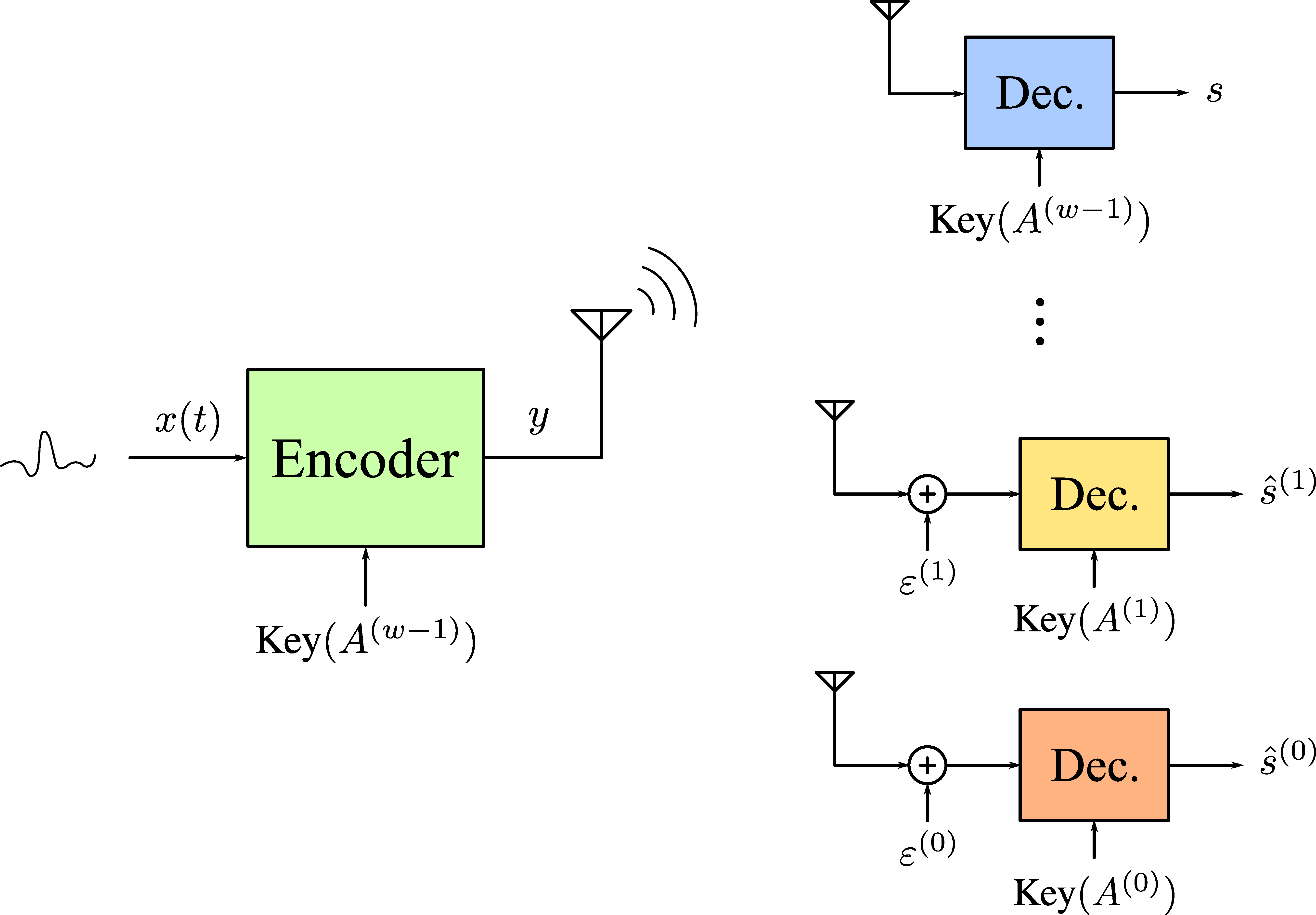
The strategy described in this section provides a multiclass encryption architecture where the shared secret between the CS encoder and each receiver is distributed depending on the quality level granted to the latter.
In particular, the full encryption key of a -class CS system is composed of seeds, i.e. low-class users are provided the secret , class- users are provided up to high-class users with . A sample network scenario is depicted in Fig. 1.
From the resources point of view, multiclass CS can be enabled with very small computational overhead. The encoding matrix generator is the same at both the encoder and high-class decoder side, whereas lower-class decoders may use the same generation scheme but are unable to rebuild the true encoding due to the missing private keys .
The initial matrix is updated from a pseudorandom binary stream generated by expanding with a PRNG. The introduction of sign-flipping is a simple post-processing step carried out on the stream buffer by reusing the same PRNG architecture and expanding the corresponding , thus having minimal computational cost.
Since the values generated by this PRNG are never exposed, cryptographically secure generators may be avoided, provided that the period with which the matrices are reused is kept sufficiently large – this requirement is crucial to avoid attacks that could exploit multiple plaintext-ciphertext pairs to fully or partially recover the encoding matrix.
II-E Lower-Class Recovery Performance Bounds
In order to quantify the recovery quality performance gap between low- and high-class users receiving the same CS measurements from the network of Fig. 1, we now provide performance bounds on the recovery error in the simple two-class case, starting from the basic intuition that if the sparsity basis of is not the canonical basis, then most plaintexts , so the perturbation noise .
II-E1 Second-Class Recovery Error – Lower Bound
The following results aim at predicting the best-case recovery quality of any second-class decoder that assumes was encoded by , whereas in absence of other noise sources and regardless of the sparsity of .
Theorem 1 (Second-class recovery error lower bound).
Let:
- 1.
-
2.
be as in with finite , and be the corresponding measurements’ RV;
For all and any instance , any that satisfies is such that the recovery error norm
| (6) |
with probability
| (7) |
where denotes the maximum singular value of its argument.
Corollary 1 (Asymptotic case of Theorem 1).
Let:
-
1.
be as in Theorem 1 as ;
-
2.
be as in , -mixing [23, (27.25)], with finite and uniformly bounded for some . Denote with the corresponding measurements’ RP of instances ;
For all and , any that satisfies is such that the recovery error power
| (8) |
with probability .
The proof of these statements is given in Appendix A. Simply put, Theorem 1 and Corollary 1 state that a second-class decoder recovering such that is subject to a recovery error whose norm, with high probability, exceeds a quantity depending on the density of the perturbation , the undersampling rate and the average energy or power respectively. In particular, the non-asymptotic case in (6) is a probabilistic lower bound: as a quantitative example, by assuming it holds with probability and that (see [24]) one could take an arbitrary to obtain w.r.t. RVs having average energy . In other words, with probability a perturbation of density will cause a minimum recovery error norm of .
A stronger asymptotic result holding with probability on is then reported in Corollary 1 under mild assumptions on the RP , where can be arbitrarily close to and only affecting the convergence rate to this lower bound. The bounds in (6) and (8) are adopted as reference best-cases in absence of other noise sources for the second-class decoder, which exhibits higher recovery error for most problem instances and reconstruction algorithms as detailed in Section IV.
II-E2 Second-Class Recovery Error – Upper Bound
We now derive a second-class recovery error upper bound by applying the theory in [13] which extends the well-known recovery guarantees in [21] to a perturbed encoding matrix model identical to (2). While adaptations exist [25] none tackle the unstructured, i.i.d. sparse random perturbation of (3) which we will now model.
The framework of [13] analyses the recovery error upper bound when using as the encoding matrix in the reference basis pursuit with denoising (BPDN) problem
| () |
for a given noise parameter . Let denote the extreme singular values among all -column submatrices of a matrix, and define the perturbation-related constants
| (9) |
and the well-known restricted isometry constant (RIC, [22]) . We estimate and plug these quantities in the upper bound of [13, Theorem 2]. For the sake of simplicity, we report it below in the case of plaintexts having exactly -sparse representations in absence of other noise sources.
Proposition 1 (Second-class recovery error upper bound, adapted from [13]).
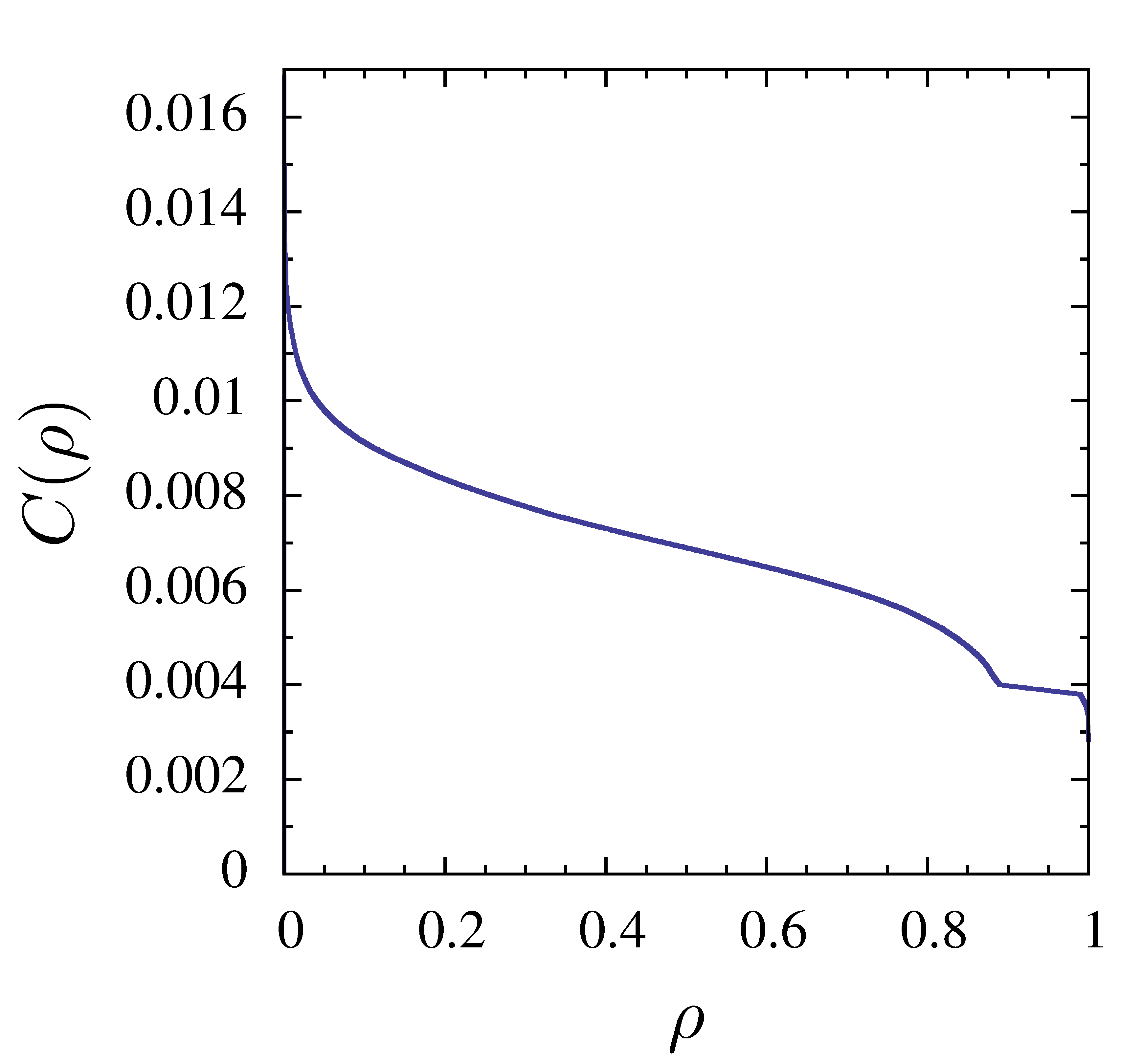
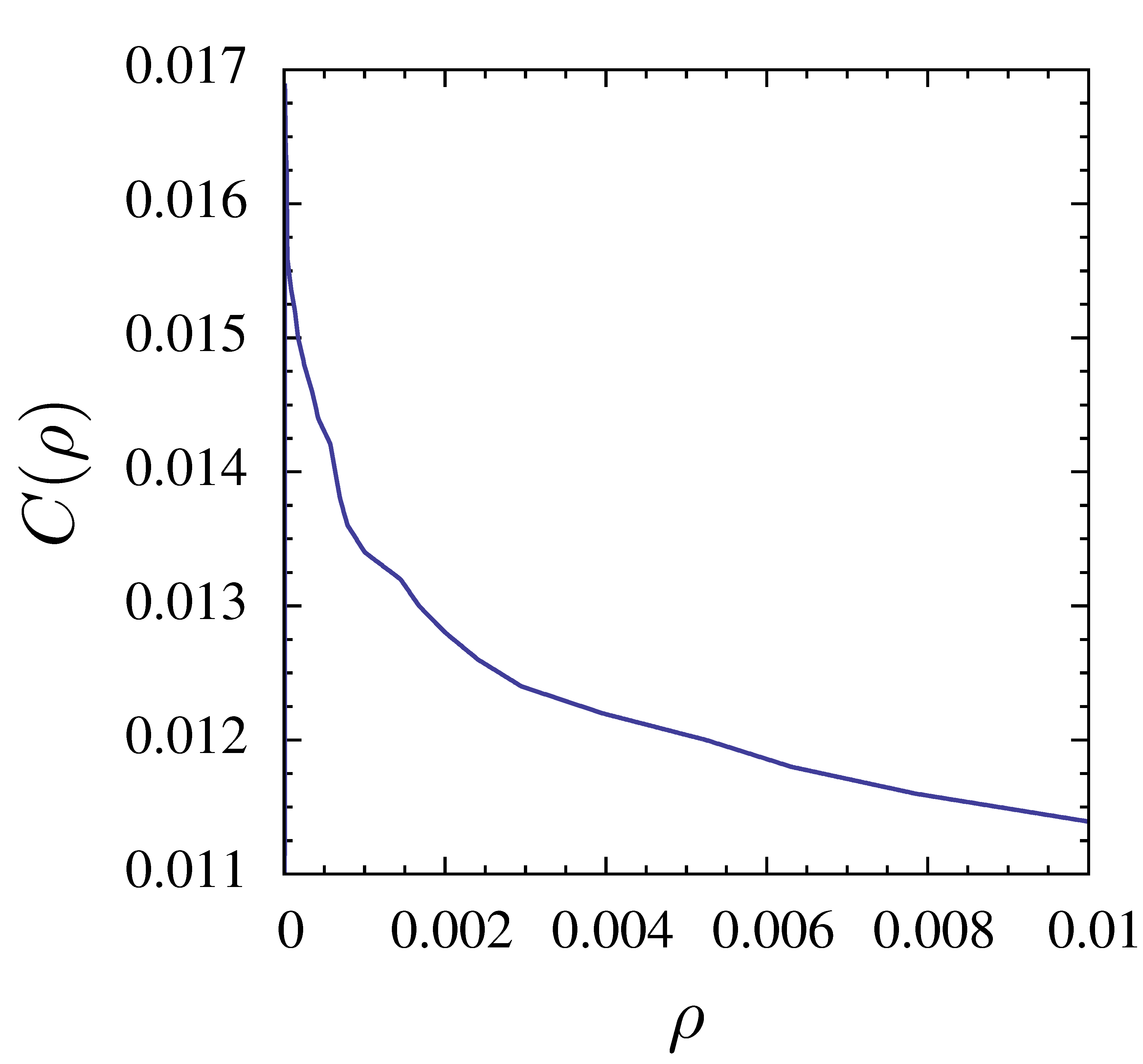
Such a guarantee depends on : theoretical results exist for estimating their value by bounding the maximum singular values in (9) since the entries of and are i.i.d. (in particular, [24] applies to , [26] to ). Yet, they would hold only when is the identity and involve universal constants whose values would require numerical evaluation. For these reasons we choose to estimate the required quantities directly by Monte Carlo simulation.
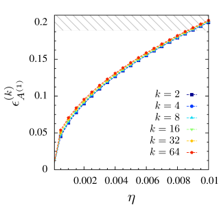
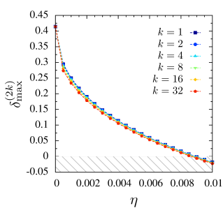
As an example, we calculate (9) for instances of submatrices of and with and . This allows us to find typical values of as reported in Fig. 2a. In the same setting only when . In Fig. 2b we report the corresponding range of allowed RIC that comply with Proposition 1, i.e. the RIC constraints the encoding matrices must meet so that (10) holds.
Such RIP-based analyses provide very strong sufficient conditions for signal recovery (see [27, Section X]) which in our case result in establishing a formal upper bound for a small range of and when solving (). As observed by the very authors of [13], typical recovery errors are substantially smaller than this upper bound. We will therefore rely on another less rigorous, yet practically effective least-squares approach using the same hypotheses of Theorem 1 to bound the average recovery quality performances in Section IV.
III A Cryptanalysis of Compressed Sensing
Consider a generic CS scheme as in Section II-A with linearly encoding a plaintext into a ciphertext . We now investigate the security properties and limits of such random linear measurements by letting be realisations of either RVs or RPs with their respective a priori distributions as in the classic Shannon framework [28].
III-A Security Limits
The encoding performed by CS is a linear mapping, and as such it cannot completely hide the information contained in a plaintext . This has two main consequences: firstly, linearity propagates scaling. Hence, it is simple to distinguish a plaintext from another if one knows that for some scalar . For the particular choice this leads to a known argument [12, Lemma 1] against the fundamental requirement for perfect secrecy that the conditional PDF (e.g. in model ). In the following, we will prove that a scaling factor is actually all that can be inferred from the statistical analysis of CS-encoded ciphertexts.
Secondly, linearity implies continuity. Hence, whenever and are close to each other for a fixed , the corresponding and will also be close to each other. This fact goes against the analog version of the diffusion (or avalanche effect) requirement for digital-to-digital ciphers [29]. If the encoding process did not entail a dimensionality reduction, this fact could be exploited every time a plaintext-ciphertext pair is known. If a new ciphertext is available that is close to , then it is immediately known that the corresponding plaintext must be close to thus yielding a good starting point for e.g. a brute-force attack.
The fact that slightly complicates this setting since the counterimages of through belong to a whole subspace in which points arbitrarily far from exist in principle. Yet, encoding matrices are chosen by design so that the probability of their null space aligning with and (that are -sparse w.r.t. a certain ) is overwhelmingly small [22]. Hence, even if with some relaxation from the quantitative point of view, neighbouring ciphertexts strongly hint at neighbouring plaintexts. As an objection to this seemingly unavoidable issue note that the previous argument only holds when the encoding matrix remains the same for both plaintexts, while by our assumption (Section II-B) on the very large period of the generated sequence of encoding matrices two neighbouring plaintexts will most likely be mapped by different encoding matrices to non-neighbouring ciphertexts .
III-B Achievable Security Properties
III-B1 Asymptotic Security
While perfect secrecy is unachievable, we may introduce the notion of asymptotic spherical secrecy and show that CS with universal random encoding matrices has this property, i.e. no information can be inferred on a plaintext in model from the statistical properties of all its possible ciphertexts but its power. The implication of this property is the basic guarantee that a malicious eavesdropper intercepting the measurement vector will not be able to extract any information on the plaintext except for its power.
Definition 1 (Asymptotic spherical secrecy).
Let be a RP whose plaintexts have finite power , be a RP modelling the corresponding ciphertexts. A cryptosystem has asymptotic spherical secrecy if for any of its plaintexts and ciphertexts we have
| (11) |
where denotes convergence in distribution as , denotes conditioning over plaintexts with the same power .
From an eavesdropper’s point of view, asymptotic spherical secrecy means that given any ciphertext we have
implying that any two different plaintexts with an identical, prior and equal power remain approximately indistinguishable from their ciphertexts. In the asymptotic setting, the following proposition holds.
Proposition 2 (Asymptotic spherical secrecy of random measurements).
Let be a RP with bounded-value plaintexts of finite power , any variable of the RP as in . For we have
| (12) |
Thus, universal encoding matrices provide independent, asymptotically spherical-secret measurements as in (11).
The proof of this statement is given in Appendix B. Since the rows of are independent, the measurements conditioned only on are also independent and Proposition 2 asserts that, although not secure in the Shannon sense, CS with suitable encoding matrices is able to conceal the plaintext up to the point of guaranteeing its security for .
As a more empirical illustration of spherical secrecy for finite , we consider an attack aiming at distinguishing two orthogonal plaintexts and from their encryption (clearly, finite energy must be assumed as in ). The attacker has access to a large number of ciphertexts collected in a set obtained by applying different, randomly chosen encoding matrices to a certain as in (1). Then, the attacker collects another set of ciphertexts, all of them corresponding either to or to , and must tell which is the true plaintext between the two.
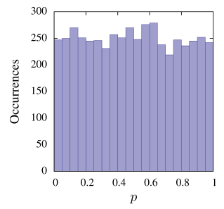
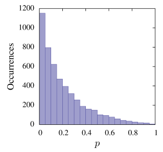
This reduces the attack to an application of statistical hypothesis testing, the null assumption being that the distribution underlying the samples in is the same as that underlying the samples in . For maximum reliability we adopt a two-level testing approach: we repeat the above experiment for many instances of random orthogonal plaintexts and , performing a two-way Kolmogorov-Smirnov (KS) test to compare the empirical distributions obtained from and produced by such orthogonal plaintexts.
Each of the above tests yields a -value quantifying the probability that two data sets coming from the same distribution exhibit larger differences w.r.t. those at hand. Given their meaning, individual -values could be compared against a desired significance level to give a first assessment whether the null hypothesis (i.e. equality in distribution) can be rejected. Yet, since it is known that -values of independent tests on distributions for which the null assumption is true must be uniformly distributed in we collect of them and feed this second-level set of samples into a one-way KS test to assess uniformity at the standard significance level .
This testing procedure is done for in the cases (same energy plaintexts) and , i.e. with a difference in energy between the two plaintexts. The resulting -values for are computed by matching pairs of sets containing ciphertexts, yielding the -value histograms depicted in Figure 3. We report the histograms of the -values in the two cases along with the -value of the second-level assessment, i.e. the probability that samples from a uniform distribution exhibit a deviation from a flat histogram larger than the observed one. When the two plaintexts have the same energy, all evidence concurs to say that the ciphertext distributions are statistically indistinguishable. In the second case, even a small difference in energy causes statistically detectable deviations and leads to a correct inference of the true plaintext between the two.
III-B2 Non-Asymptotic Security
We have observed how asymptotic spherical secrecy has finite effects (for additional evidence by numerical computation of the Kullback-Leibler divergence see [15]). From a more formal point of view, we may evaluate the convergence rate of (12) for finite to obtain some further guarantee that an eavesdropper intercepting the measurements will observe samples of an approximately Gaussian RV bearing very little information in addition to the energy of the plaintext. We hereby consider a RV as in , for which a plaintext of energy lies on the sphere of (with radius ).
The most general convergence rate for sums of i.i.d. random variables is given by the well-known Berry-Esseen Theorem [30] as . In our case we apply a recent, remarkable result of [17] that improves and extends this convergence rate to inner products of i.i.d. RVs (i.e. any row of ) and vectors (i.e. plaintexts ) uniformly distributed on .
Proposition 3 (Rate of convergence of random measurements).
Let be RVs as in with a random matrix of i.i.d. zero mean, unit variance, finite fourth moment entries. For any , there exists a subset with probability measure such that if then all in verify
| (13) |
for a non-increasing function of .
Proposition 3 with sufficiently small means that it is most likely (actually, with probability exceeding ) to observe an convergence between and the limiting distribution . The function is loosely bounded in [17], so to complete this analysis we performed a thorough Monte Carlo evaluation of its possible values. In particular, we have taken instances of a RV uniformly distributed on for each . The PDF is estimated with the following procedure: we generate rows of an i.i.d. Bernoulli random matrix and perform the linear combination in (1), thus yielding the same number of instances of for each and . On this large sample set we are able to accurately estimate the previous PDF on 4096 equiprobable intervals, and compare it to the same binning of the normal distribution as in the LHS of (13) for each . This method yields sample values for (13), allowing an empirical evaluation of the quantity . In this example, when Proposition 3 holds with .
Hence, straightforward statistical attacks on a CS-encoded ciphertext may only extract very limited information from the plaintext. Yet, other attacks may rely on a larger amount of information, the next level of threat being known-plaintext attacks [29]. These attacks are based on the availability of some plaintext-ciphertext pairs and aim at the extraction of information on the encoding process that can be reused to decode future ciphertexts. Due to its criticality and theoretical depth, the robustness of multiclass CS w.r.t. this class of attacks will be tackled in a separate contribution.
IV Application Examples
IV-A Experimental Framework
In this section we detail some example applications for the multiclass CS scheme we propose. For each example we study the recovery quality attained by first-class receivers against second-class ones in the two-class scheme (Section II-D1). These results encompass the multiclass setting since high-class receivers correspond to first-class recovery performances (i.e. ), while lower-class users attain the performances of a second-class receiver at a fixed .
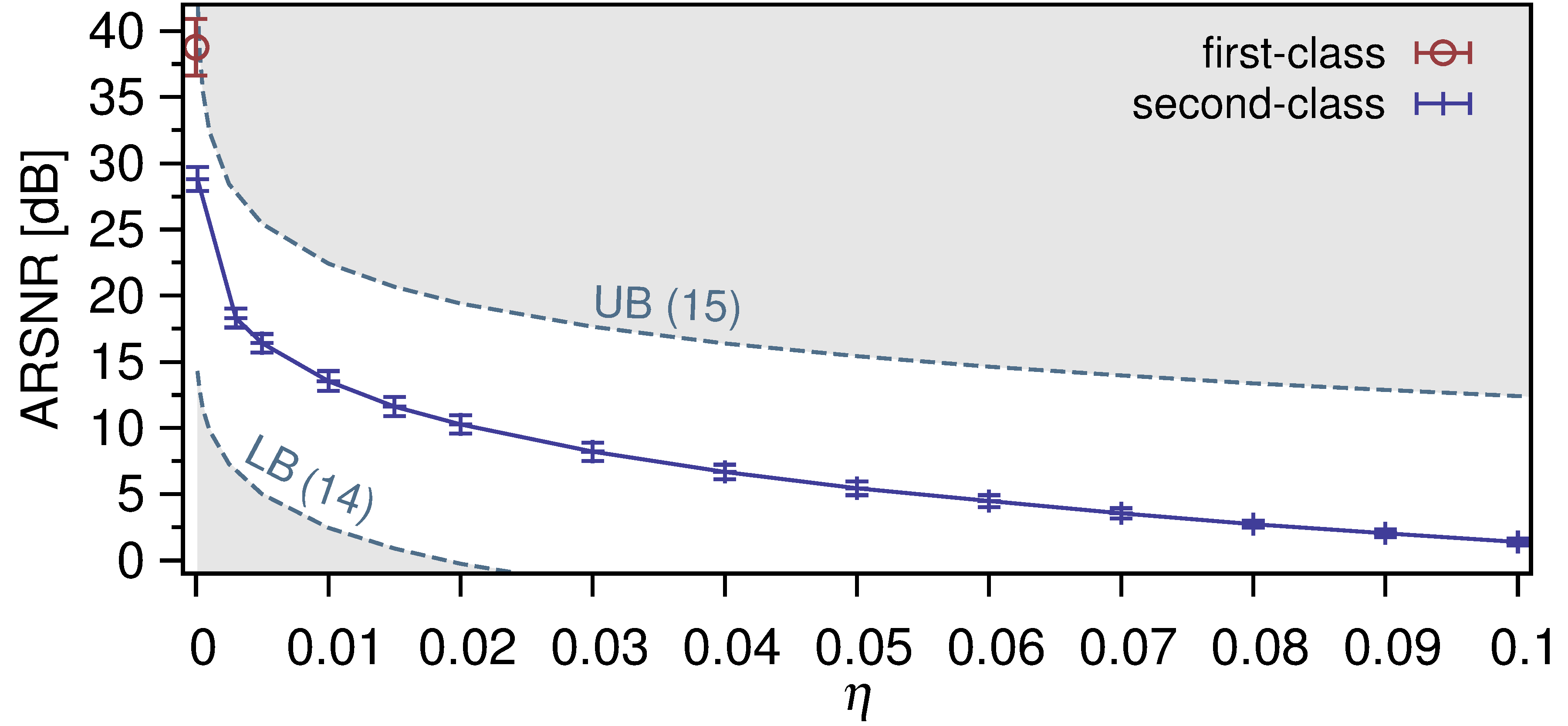
For each plaintext being reconstructed the recovery signal-to-noise ratio with denoting the recovered approximation is a common recovery quality index; its average222 denotes the sample average over a set of realisations of the argument., is then used as an average performance index, and compared against some best- and worst-case curves with the purpose of choosing a suitable perturbation density so that lower-class recovery performances are set to the desired quality level.
We complement the previous evidence with an automated assessment of the information content intelligible from by means of feature extraction algorithms. These are equivalent to partially informed attacks attempting to expose the sensitive content inferred from the recovered signal. More specifically, we will try to recover an English sentence from a speech segment, the location of the PQRST peaks in an electrocardiographic (ECG) signal, and printed text in an image. The simulation framework reproducing these tests is available at http://securecs.googlecode.com.
IV-A1 Recovery Algorithms
While fundamental sparse signal recovery guarantees are well-known from [21] when solving BP and BPDN, these convex problems are often replaced in practice by a variety of high-performance algorithms (see e.g. [31]). As reference cases for most common algorithmic classes we tested the solution of BPDN as implemented in SPGL1 [32, 33] against the greedy algorithm CoSaMP [34] and the generalised approximate message-passing algorithm (GAMP, [35]). To optimise these algorithms’ performances the tests were optimally tuned in a “genie-aided” fashion: BPDN was solved as in () with the noise parameter as if were known beforehand; CoSaMP was initialised with the exact sparsity level for each case; GAMP was run with the sparsity-enforcing, i.i.d. Bernoulli-Gaussian prior (see e.g. [36]) broadly applicable in the well-known message passing framework [37] and initialised with the exact sparsity ratio of each instance, and the exact mean and variance of each considered test set. Moreover, signal-independent parameters were hand-tuned in each case to yield optimal recovery performances.
For the sake of brevity, in each example we select and report the algorithm that yields the most accurate recovery quality at a lower-class decoder as the amount of perturbation varies. We found that GAMP achieves the highest in all the settings explored in the examples, consistently with the observations in [36] that assess the robust recovery capabilities of this algorithm under a broadly applicable sparsity-enforcing prior. Moreover, as verifies [38, Proposition 2.1] the perturbation noise is approximately Gaussian for large and thus GAMP tuned as above yields optimal performances as expected. Note that recovery algorithms which attempt to jointly identify and [38, 39] can be seen as explicit attacks to multiclass encryption and are thus evaluated in a separate contribution, anticipating that their performances are compatible with those of GAMP.
IV-A2 Average Signal-to-Noise Ratio Bounds
The perturbation density is the main design parameter for the multiclass encryption scheme, and therefore has to be chosen against a reference lower-class recovery algorithm. To provide criteria for the choice of we adopt two bounds derived as follows.
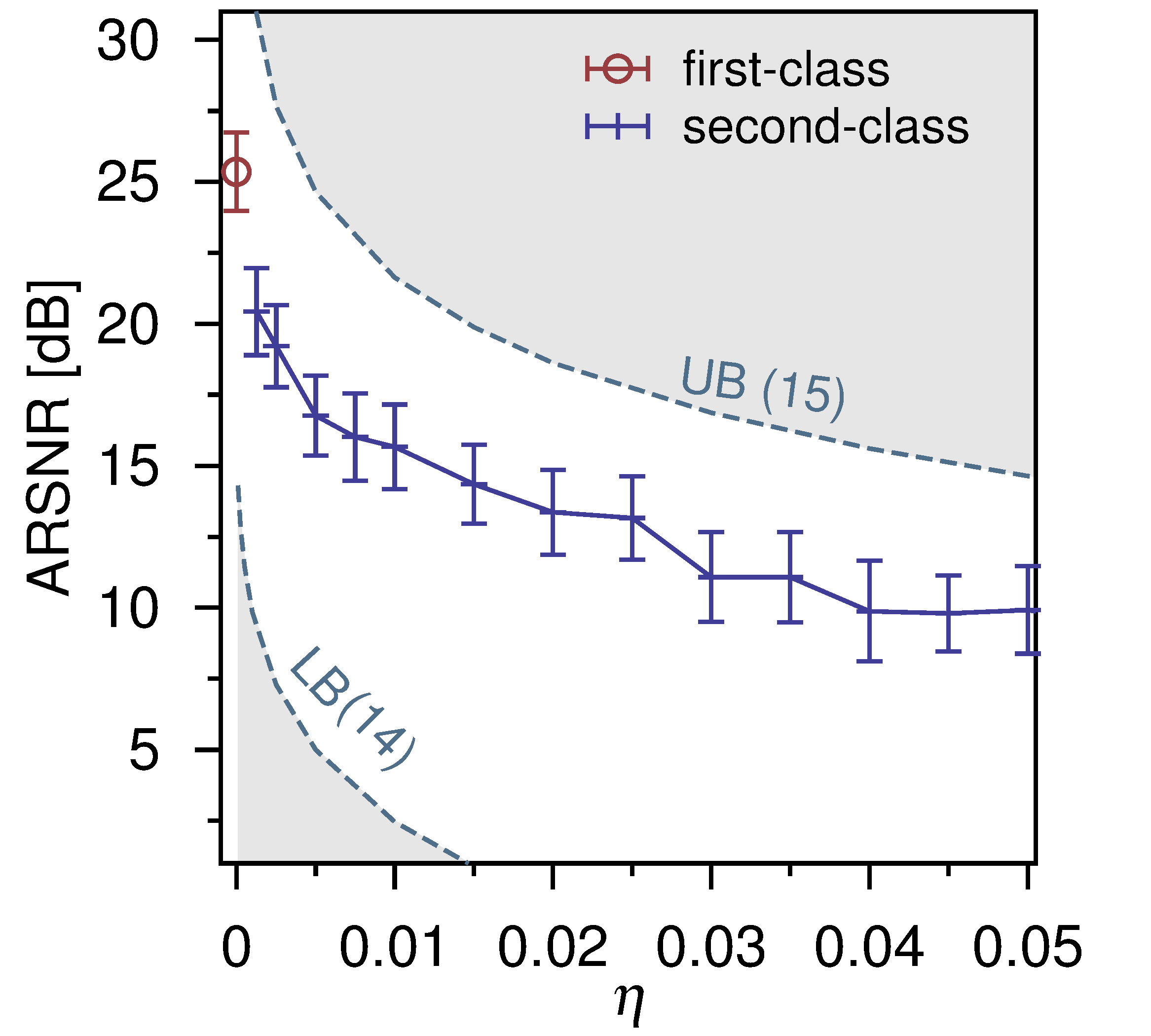
Although rigorous, the lower-class recovery error upper bound of Proposition 1 is only applicable for small values of . To bound typical recovery performances in a larger range we analyse the behaviour of a lower-class decoder that naively (i.e. without attempting any attack) recovers such that , and thus . In most cases, such a recovery produces lying close to ; we model this by assuming is close to be minimum. With this, we may approximate , where denotes the Moore-Penrose pseudoinverse, that yields . By taking a sample average on both sides, in signal-to-noise ratio our criterion is where
| (14) |
is calculated in each of the following examples by a thorough Monte Carlo simulation of over cases.
The opposite criterion is found by assuming where
| (15) |
obtained from a simple rearrangement of (8) with . We will see how (14) and (15) fit the performances of the examples and provide simple criteria to estimate the range of performances of lower-class receivers from .
IV-B Speech Signals
We consider a subset of spoken English sentences from the PTDB-TUG database [40] with original sampling frequency , variable duration and sentence length. Each speech signal is divided in segments of samples and encoded by two-class CS with measurements. We obtain the sparsity basis by applying principal component analysis [41] to -dimensional segments yielding an ONB. The encoding matrix is generated from an i.i.d. Bernoulli random matrix by adding to it a sparse random perturbation chosen as in (3) with density . The encoding in (5) is simulated in a realistic setting, where each window of samples is acquired with a different instance of yielding measurements per speech segment. As for the decoding stage, we apply GAMP as specified above to recover given (first-class) and (second-class).
For a given encoding matrix a first-class receiver is capable of decoding a clean speech signal with , whereas a second-class receiver is subject to significant degradation when increases, as shown in Fig. 5a. Note that while the for has a relative deviation of around its mean (the ), as increases the observed deviation is less than . Note how the values lie in the highlighted range between (14), (15).
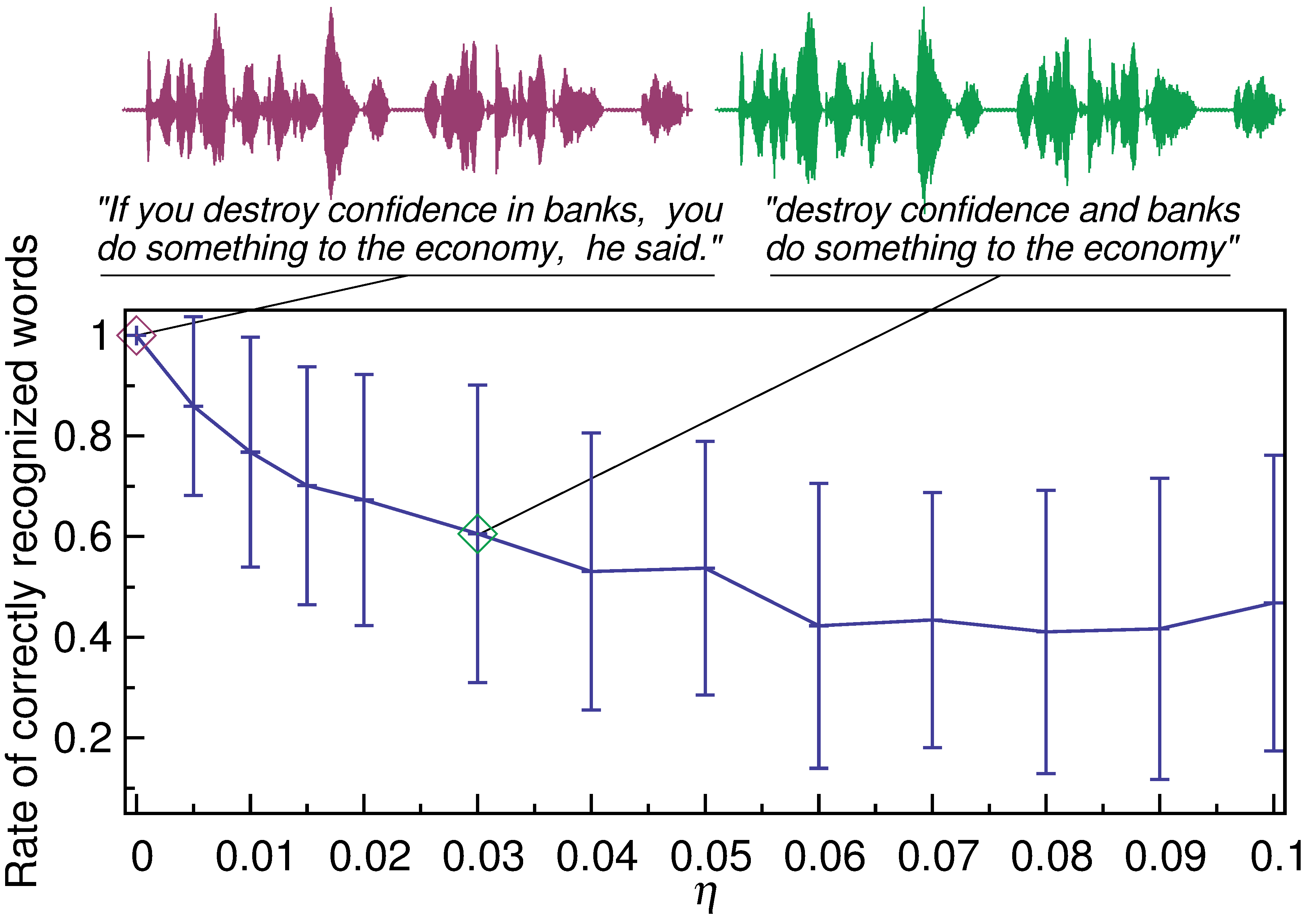
To further quantify the limited quality of attained recoveries, we process the recovered signal with the Google Web Speech API [42, 43] which provides basic Automatic Speech Recognition (ASR). The ratio of words correctly inferred by ASR for different values of is reported in Fig. 5b. This figure also reports a typical decoding case: a first-class user (i.e. ) recovers the signal with , whereas a second-class decoder only achieves a when . The corresponding ratio of recognised words is against . In both cases the sentence is intelligible to a human listener, but the second-class decoder recovers a signal that is sufficiently corrupted to avoid straightforward ASR.
IV-C Electrocardiographic Signals
We extend the example in [15] by processing a large subset of ECG signals from the MIT PhysioNet database [44] sampled at . In particular, we report the case of a typical minutes ECG track (sequence e0108) and encode windows of samples by two-class CS with measurements, amounting to a dataset of ECG instances.
The encoding and decoding stages are identical to those in Section IV-B and we assume the Symmlet-6 ONB [45] as the sparsity basis .
In this setting, the first-class decoder is able to reconstruct the original signal with , whereas a second-class decoder subject to a perturbation of density achieves an ; the recovery degradation depends on as reported in Fig. 6a.
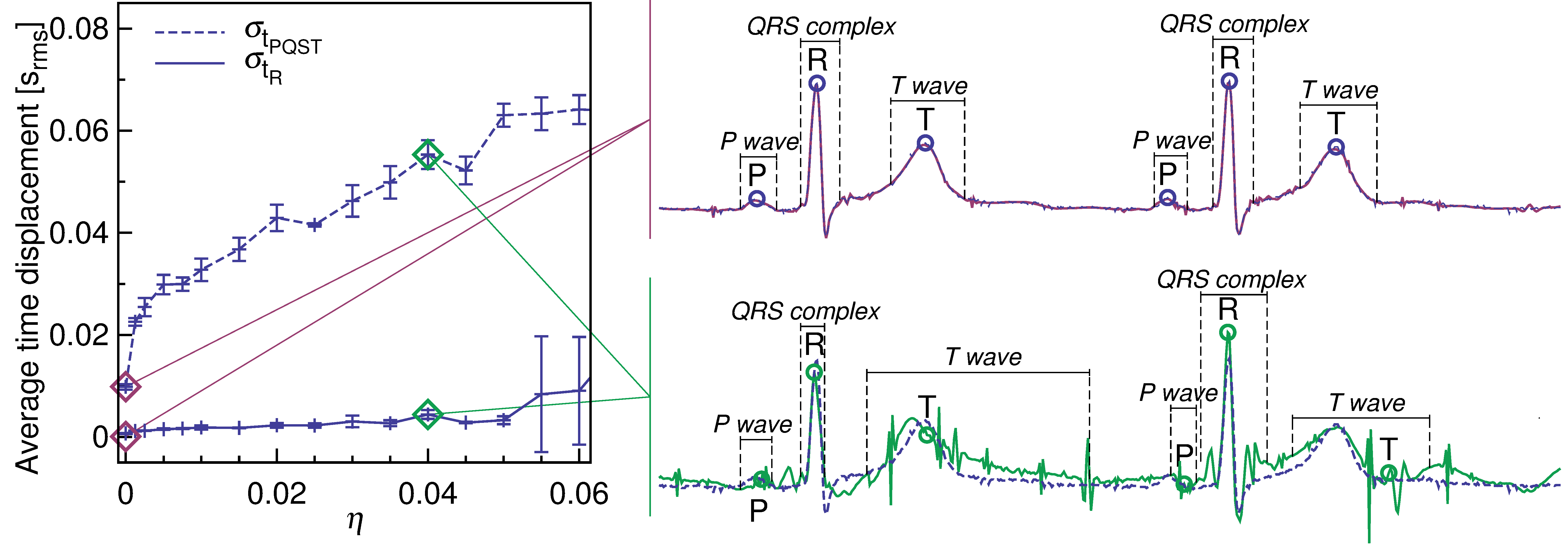
As an additional quantification of the encryption at second-class decoders we apply PUWave [46], an Automatic Peak Detection algorithm (APD), to first- and second-class signal reconstructions. In more detail, PUWave is used to detect the position of the P,Q,R,S and T peaks, i.e. the sequence of pulses whose positions and amplitudes summarise the diagnostic properties of an ECG. The application of this APD yields the estimated peak instants for each of reconstructed windows and each decoder class, which are afterwards compared to the corresponding peak instants as detected on the original signal prior to encoding. Thus, we define the average time displacement and evaluate it for and . A first-class receiver is subject to a displacement of the R-peak and of the remaining peaks w.r.t. the original signal. On the other hand, a second-class user is able to determine the R-peak with while the displacement of the other peaks is . As varies in this displacement increases as depicted in Fig. 6b, thus confirming that a second-class user will not be able to accurately determine the position and amplitude of the peaks with the exception of the R-peak.
IV-D Sensitive Text in Images
In this final example we consider an image dataset of people holding printed identification text and apply multiclass CS to selectively hide this sensitive content to lower-class users. The images are encoded by CS in each of while the two-class strategy is only applied to a relevant image area of . We adopt as sparsity basis the 2D Daubechies-4 wavelet basis [45] and encode each block of with measurements; the encoding is generated with perturbation density .
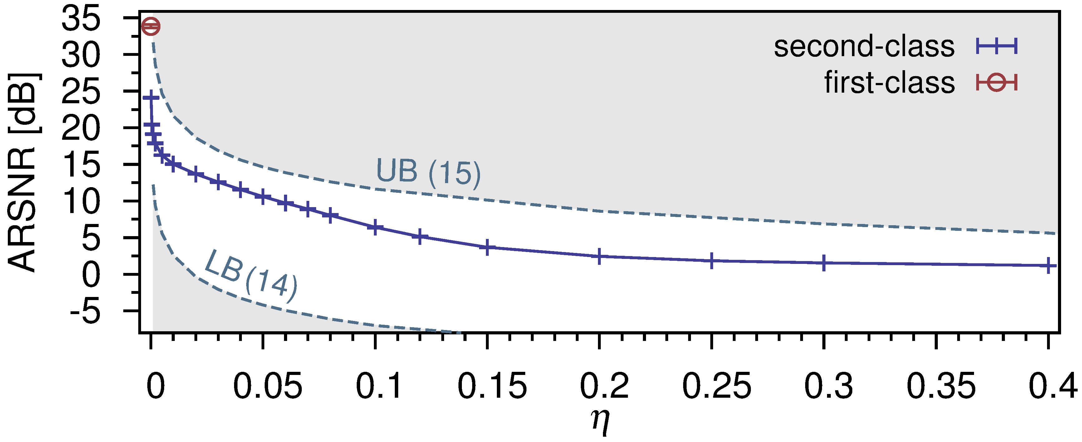
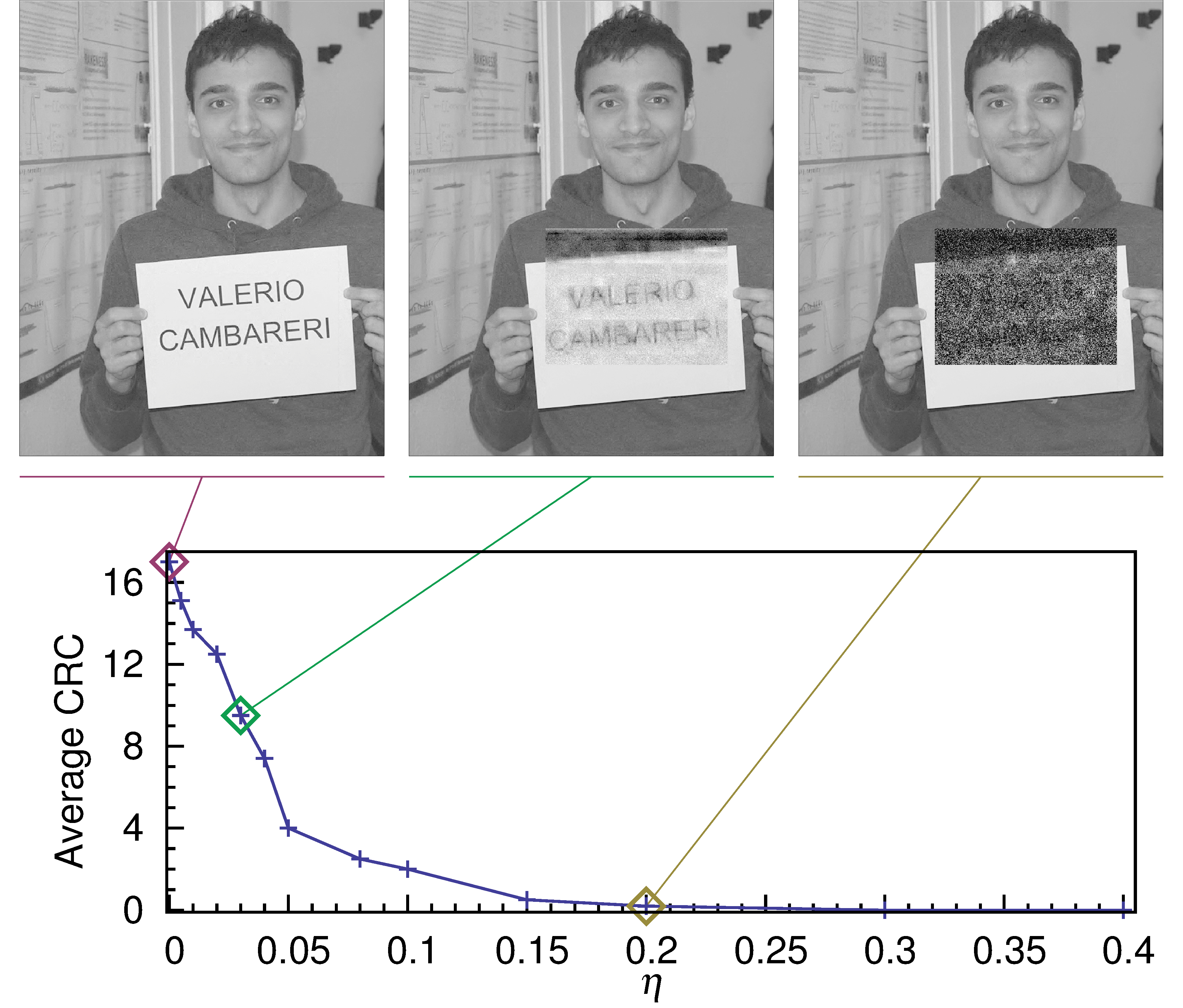
The performances of this example are reported in Fig. 7a as averaged on 20 instances per case, showing a rapid degradation of the as is increased. This degradation is highlighted in the typical case of Fig. 7b for .
In order to assess the effect of our encryption method with an automatic information extraction algorithm, we have applied Tesseract [47], an optical character recognition (OCR) algorithm, to the images reconstructed by a second-class user. The text portion in the recovered image data is preprocessed to enhance their quality prior to OCR: the images are first rotated, then we apply standard median filtering to reduce the highpass noise components. Finally, contrast adjustment and thresholding yield the two-level image which is processed by Tesseract. To assess the attained OCR quality we have measured the average number of consecutive recognised characters (CRC) from the decoded text image. In Fig. 7b the average CRC is reported as a function of : as the perturbation density increases the OCR fails to recognise an increasing number of ordered characters, i.e. a second-class user progressively fails to extract text content from the decoded image.
V Conclusion
Although not perfectly secure, the extremely simple encoding process entailed by CS yields some encryption capabilities with no additional computational complexity, thus providing a limited but zero-cost form of encryption which might be of interest in the design of secure yet resource-limited sensing interfaces. In particular, we have shown that when i.i.d. Bernoulli random matrices are used in this linear encoding scheme the plaintext features that leak into the ciphertext (and therefore retrievable by statistical analysis of the latter) are limited to the power of the plaintext as , and thus how an asymptotic definition of secrecy holds for this scheme. In addition, we have given evidence of the convergence rate to this limit behaviour. We have also detailed how two plaintexts having the same energy and encoded with an i.i.d. Bernoulli random matrix generate statistically indistinguishable ciphertexts, while even small differences in energy are detected by hypothesis testing on the ciphertext for finite . The above linear random encoding was modified to envision a multiclass encryption scheme in which all receivers are given the same set of measurements, but are only enabled to reconstruct the original signal with a decoding quality that depends on their class, i.e. on the private key they possess. This additional design option amounts to the ability of flipping pseudo-randomly chosen elements of the encoding matrix, and thus represents an appealing alternative to balance the trade-off between the security of the encoded signal and the resources required to provide it.
Finally, the capabilities of multiclass CS were exemplified by simulating the acquisition of sources such as speech segments, electrocardiographic signals and images with the additional security provided by the devised encryption method.
Appendix A Proofs regarding the Second-Class
Recovery Error Lower Bound
We first introduce a Lemma that gives a self-contained probabilistic result on the Euclidean norm of in (5); this is used in the proofs of Theorem 1 and Corollary 1.
Lemma 1.
Let:
-
1.
be a RV with , ;
-
2.
be the sparse random matrix in (3) with i.i.d. entries and density .
If and are independent, then for any
| (16) |
with
| (17) |
Proof of Lemma 1. Consider
We now derive the first and second moments of this positive RV. is a random matrix of i.i.d. RVs with mean , variance and . Using the independence between and , and the fact that is i.i.d. we have
For the aforementioned properties of we also have
that can be used in some cumbersome but straightforward calculations yielding
where . We are now in the position of using a one-sided version of Chebyshev’s inequality for positive RVs333If a r.v. then , . to say that, for any ,
which yields (17) by considering that when , . ∎
Proof of Theorem 1. Since all decoders receive in absence of other noise sources the same measurements , a second-class decoder would naively assume , with an approximation of obtained by a recovery algorithm that satisfies this equality. Since , if we define we may write and thus . can then be bounded straightforwardly as yielding
| (18) |
By applying the probabilistic lower bound of Lemma 1 on in (18), we have that for and a given probability value exceeding in (17). Plugging the RHS of this inequality in (18) yields (6). ∎
The following Lemma applies to finding the asymptotic result (8) of Corollary 1.
Lemma 2.
Let be an -mixing RP with uniformly bounded fourth moments for some . Define ms .
If then .
Proof of Lemma 2. Note first that from Jensen’s inequality , so also implies that and . Since we may write
| (19) |
and observe that where . From the -mixing assumption we know that and a sequence vanishing as . Hence,
| (20) |
The thesis follows from the fact that the upper bound in (20) vanishes as . This is obvious when is convergent. Otherwise, if is divergent we may resort to the Stolz-Cesàro theorem to find . ∎
Proof of Corollary 1. The inequality (18) in the proof of Theorem 1 is now modified for the asymptotic case of a RP . Note that is an i.i.d. random matrix with zero mean, unit variance entries; thus, when with the value is known from [48] since all the singular values belong to the interval . We therefore assume and take the limit of (18) normalised by for , yielding
| (21) |
with the -th finite-length term in a plaintext of . We may now apply Lemma 1 in for each at the numerator of the RHS of (21) with , and as in Lemma 1. For and , the probability in (17) becomes
Since satisfies by hypothesis the assumptions of Lemma 2, then and . Hence, with and probability the RHS of (21) becomes
and the recovery error power satisfies (8). ∎
Appendix B Proofs regarding the Spherical Secrecy
of Compressed Sensing
Proof of Proposition 2. The proof is given by simple verification of the Lindeberg-Feller central limit theorem (see [23, Theorem 27.4]) for in conditioned on a plaintext of in . By the hypotheses, the plaintext has power and for some finite . Any where is a sequence of independent, non-identically distributed random variables of moments . By letting the partial sum , its mean and . Thus, we verify the necessary and sufficient condition [23, (27.19)]
by straightforwardly observing
The verification of this condition guarantees that is normally distributed with variance , i.e. . ∎
Proof of Proposition 3. We start by considering in of model conditioned on a given with finite energy . Each of such variables is a linear combination (1) of i.i.d. RVs with zero mean, unit variance and finite fourth moments. The coefficients of this linear combination are which by now we assume to have , i.e. to lie on the unit sphere of . Define , which for i.i.d. Bernoulli random matrices is , whereas for standard random matrices . This setting verifies [17, Theorem 1.1]: for any there exists a subset with measure such that and if , then
| (22) |
with a positive, non-increasing function. An application of this result to with energy , i.e. on the sphere of radius , ( i.i.d. Bernoulli) can be done by straightforwardly scaling the standard normal PDF in (22) to , thus yielding the statement of Proposition 3. ∎
References
- [1] I. F. Akyildiz, W. Su, Y. Sankarasubramaniam, and E. Cayirci, “A survey on sensor networks,” Communications magazine, IEEE, vol. 40, no. 8, pp. 102–114, 2002.
- [2] Y. Wang, G. Attebury, and B. Ramamurthy, “A survey of security issues in wireless sensor networks,” Communications Surveys & Tutorials, IEEE, vol. 8, no. 2, pp. 2–23, 2006.
- [3] J. Daemen and V. Rijmen, The design of Rijndael: AES-the advanced encryption standard. Springer, 2002.
- [4] D. L. Donoho, “Compressed Sensing,” IEEE Transactions on Information Theory, vol. 52, no. 4, pp. 1289–1306, Apr. 2006.
- [5] E. J. Candès and M. B. Wakin, “An Introduction to Compressive Sampling,” IEEE Signal Processing Magazine, vol. 25, no. 2, pp. 21–30, Mar. 2008.
- [6] J. A. Tropp, J. N. Laska, M. F. Duarte, J. K. Romberg, and R. G. Baraniuk, “Beyond nyquist: Efficient sampling of sparse bandlimited signals,” Information Theory, IEEE Transactions on, vol. 56, no. 1, pp. 520–544, 2010.
- [7] M. Mishali, Y. C. Eldar, and A. J. Elron, “Xampling: Signal acquisition and processing in union of subspaces,” Signal Processing, IEEE Transactions on, vol. 59, no. 10, pp. 4719–4734, 2011.
- [8] J. Haboba, M. Mangia, F. Pareschi, R. Rovatti, and G. Setti, “A pragmatic look at some compressive sensing architectures with saturation and quantization,” Emerging and Selected Topics in Circuits and Systems, IEEE Journal on, vol. 2, no. 3, pp. 443–459, Sept.
- [9] M. F. Duarte, M. A. Davenport, D. Takhar, J. N. Laska, T. Sun, K. F. Kelly, and R. G. Baraniuk, “Single-pixel imaging via compressive sampling,” Signal Processing Magazine, IEEE, vol. 25, no. 2, pp. 83–91, 2008.
- [10] F. Chen, A. Chandrakasan, and V. Stojanovic, “Design and analysis of a hardware-efficient compressed sensing architecture for data compression in wireless sensors,” Solid-State Circuits, IEEE Journal of, vol. 47, no. 3, pp. 744–756, 2012.
- [11] E. J. Candès and T. Tao, “Near-optimal signal recovery from random projections: Universal encoding strategies?” Information Theory, IEEE Transactions on, vol. 52, no. 12, pp. 5406–5425, 2006.
- [12] Y. Rachlin and D. Baron, “The Secrecy of Compressed Sensing Measurements,” in 46th Annual Allerton Conference on Communication, Control, and Computing, Sep. 2008, pp. 813–817.
- [13] M. Herman and T. Strohmer, “General deviants: An analysis of perturbations in compressed sensing,” IEEE Journal of Selected Topics in Signal Processing, vol. 4, no. 2, pp. 342–349, 2010.
- [14] A. Orsdemir, H. O. Altun, G. Sharma, and M. F. Bocko, “On the security and robustness of encryption via compressed sensing,” in Military Communications Conference, 2008. MILCOM 2008. IEEE. IEEE, 2008, pp. 1–7.
- [15] V. Cambareri, J. Haboba, F. Pareschi, R. Rovatti, G. Setti, and K. W. Wong, “A two-class information concealing system based on compressed sensing,” in Circuits and Systems (ISCAS), 2013 IEEE International Symposium on. IEEE, 2013, pp. 1356–1359.
- [16] M. Zhang, M. Kermani, A. Raghunathan, and N. Jha, “Energy-efficient and secure sensor data transmission using encompression,” in VLSI Design and 2013 12th International Conference on Embedded Systems (VLSID), 2013 26th International Conference on, 2013, pp. 31–36.
- [17] B. Klartag and S. Sodin, “Variations on the Berry – Esseen Theorem,” Theory of Probability & Its Applications, vol. 56, no. 3, pp. 403–419, 2012.
- [18] P.-L. Loh and M. J. Wainwright, “Corrupted and missing predictors: Minimax bounds for high-dimensional linear regression,” in Information Theory Proceedings (ISIT), 2012 IEEE International Symposium on, July 2012, pp. 2601–2605.
- [19] ——, “High-dimensional regression with noisy and missing data: Provable guarantees with nonconvexity,” Annals of Statistics, vol. 40, no. 3, p. 1637, 2012.
- [20] E. J. Candès and T. Tao, “Decoding by linear programming,” IEEE Transactions on Information Theory, vol. 51, no. 12, pp. 4203–4215, Dec. 2005.
- [21] E. J. Candès, J. K. Romberg, and T. Tao, “Stable signal recovery from incomplete and inaccurate measurements,” Communications on Pure and Applied Mathematics, vol. 59, no. 8, pp. 1207–1223, Aug. 2006.
- [22] E. J. Candès, “The restricted isometry property and its implications for compressed sensing,” Comptes Rendus Mathematique, vol. 346, no. 9, pp. 589–592, 2008.
- [23] P. Billingsley, Probability and measure. John Wiley & Sons, 2008.
- [24] M. Rudelson and R. Vershynin, “Non-asymptotic theory of random matrices: extreme singular values,” in Proceedings of the International Congress of Mathematicians. Citeseer, 2010.
- [25] Z. Yang, C. Zhang, and L. Xie, “Robustly stable signal recovery in compressed sensing with structured matrix perturbation,” Signal Processing, IEEE Transactions on, vol. 60, no. 9, pp. 4658–4671, 2012.
- [26] R. Latała, “Some estimates of norms of random matrices,” Proceedings of the American Mathematical Society, vol. 133, no. 5, pp. 1273–1282, 2005.
- [27] D. Donoho and J. Tanner, “Precise undersampling theorems,” Proceedings of the IEEE, vol. 98, no. 6, pp. 913–924, june 2010.
- [28] C. E. Shannon, “Communication Theory of Secrecy Systems,” Bell System Technical Journal, vol. 28, no. 4, pp. 656–715, Oct. 1949.
- [29] L. C. Washington and W. Trappe, Introduction to cryptography: with coding theory. Prentice Hall PTR, 2002.
- [30] A. C. Berry, “The accuracy of the gaussian approximation to the sum of independent variates,” Transactions of the American Mathematical Society, vol. 49, no. 1, pp. 122–136, 1941.
- [31] J. A. Tropp and S. J. Wright, “Computational methods for sparse solution of linear inverse problems,” Proceedings of the IEEE, vol. 98, no. 6, pp. 948–958, 2010.
- [32] E. van den Berg and M. P. Friedlander, “Sparse optimization with least-squares constraints,” SIAM Journal on Optimization, vol. 21, no. 4, pp. 1201–1229, 2011.
- [33] ——, “SPGL1: A solver for large-scale sparse reconstruction,” June 2007, http://www.cs.ubc.ca/labs/scl/spgl1.
- [34] D. Needell and J. A. Tropp, “Cosamp: Iterative signal recovery from incomplete and inaccurate samples,” Applied and Computational Harmonic Analysis, vol. 26, no. 3, pp. 301–321, 2009.
- [35] S. Rangan, “Generalized approximate message passing for estimation with random linear mixing,” in Information Theory Proceedings (ISIT), 2011 IEEE International Symposium on. IEEE, 2011, pp. 2168–2172.
- [36] J. Vila and P. Schniter, “Expectation-maximization bernoulli-gaussian approximate message passing,” in Signals, Systems and Computers (ASILOMAR), 2011 Conference Record of the Forty Fifth Asilomar Conference on. IEEE, 2011, pp. 799–803.
- [37] D. L. Donoho, A. Maleki, and A. Montanari, “Message-passing algorithms for compressed sensing,” Proceedings of the National Academy of Sciences, vol. 106, no. 45, pp. 18 914–18 919, 2009.
- [38] J. T. Parker, V. Cevher, and P. Schniter, “Compressive sensing under matrix uncertainties: An approximate message passing approach,” in Signals, Systems and Computers (ASILOMAR), 2011 Conference Record of the Forty Fifth Asilomar Conference on. IEEE, 2011, pp. 804–808.
- [39] H. Zhu, G. Leus, and G. B. Giannakis, “Sparsity-cognizant total least-squares for perturbed compressive sampling,” Signal Processing, IEEE Transactions on, vol. 59, no. 5, pp. 2002–2016, 2011.
- [40] G. Pirker, M. Wohlmayr, S. Petrik, and F. Pernkopf, “A Pitch Tracking Corpus with Evaluation on Multipitch Tracking Scenario,” in Interspeech 2011, Florence (Italy), Aug. 27-31, 2011, pp. 1509–1512.
- [41] K. Karhunen, Über lineare Methoden in der Wahrscheinlichkeitsrechnung. Universitat Helsinki, 1947, vol. 37.
- [42] G. Shires and H. Wennborg, “Web Speech API Specification,” Oct. 2012, http://dvcs.w3.org/hg/speech-api/raw-file/tip/speechapi.html.
- [43] G. Hinton, L. Deng, D. Yu, G. E. Dahl, A.-r. Mohamed, N. Jaitly, A. Senior, V. Vanhoucke, P. Nguyen, T. N. Sainath et al., “Deep neural networks for acoustic modeling in speech recognition: the shared views of four research groups,” Signal Processing Magazine, IEEE, vol. 29, no. 6, pp. 82–97, 2012.
- [44] A. L. Goldberger, L. A. N. Amaral, L. Glass, J. M. Hausdorff, P. C. Ivanov, R. G. Mark, J. E. Mietus, G. B. Moody, C.-K. Peng, and H. E. Stanley, “PhysioBank, PhysioToolkit, and PhysioNet: Components of a new research resource for complex physiologic signals,” Circulation, vol. 101, no. 23, pp. e215–e220, 2000 (June 13).
- [45] S. Mallat, A wavelet tour of signal processing. Access Online via Elsevier, 1999.
- [46] R. Jane, A. Blasi, J. García, and P. Laguna, “Evaluation of an automatic threshold based detector of waveform limits in holter ecg with the qt database,” in Computers in Cardiology 1997. IEEE, 1997, pp. 295–298.
- [47] R. Smith, “An Overview of the Tesseract OCR Engine,” in Document Analysis and Recognition, 2007. ICDAR 2007. Ninth International Conference on, vol. 2, 2007, pp. 629–633.
- [48] S. Geman, “A limit theorem for the norm of random matrices,” The Annals of Probability, vol. 8, no. 2, pp. 252–261, 1980.
![[Uncaptioned image]](/html/1307.3360/assets/cambareri.png) |
Valerio Cambareri (S’13) received the B.S. and M.S. degree (summa cum laude) in Electronic Engineering from the University of Bologna, Italy, in 2008 and 2011 respectively. Since 2012 he is a Ph.D. student in Electronics, Telecommunications and Information Technologies at DEI – University of Bologna, Italy. In 2014 he was a visiting Ph.D. student in the Integrated Imagers team at IMEC, Belgium. His current research activity focuses on statistical and digital signal processing, compressed sensing and computational imaging. |
![[Uncaptioned image]](/html/1307.3360/assets/mangia.png) |
Mauro Mangia (S’09-M’13) received the B.S. and M.S. degree in Electronic Engineering from the University of Bologna, Italy, in 2004 and 2009 respectively; he received the Ph.D. degree in Information Technology from the University of Bologna in 2013. He is currently a post-doc researcher in the statistical signal processing group of ARCES – University of Bologna, Italy. In 2009 and 2012 he was a visiting Ph.D. student at the École Polytechnique Fédérale de Lausanne (EPFL). His research interests are in nonlinear systems, compressed sensing, ultra-wideband systems and system biology. He was recipient of the 2013 IEEE CAS Society Guillemin-Cauer Award and the best student paper award at ISCAS2011. |
![[Uncaptioned image]](/html/1307.3360/assets/pareschi.png) |
Fabio Pareschi (S’05-M’08) received the Dr. Eng. degree (with honours) in Electronic Engineering from University of Ferrara, Italy, in 2001, and the Ph.D. in Information Technology under the European Doctorate Project (EDITH) from University of Bologna, Italy, in 2007. He is currently an Assistant Professor in the Department of Engineering (ENDIF), University of Ferrara. He is also a faculty member of ARCES – University of Bologna, Italy. He served as Associate Editor for the IEEE Transactions on Circuits and Systems – Part II (2010-2013). His research activity focuses on analog and mixed-mode electronic circuit design, statistical signal processing, random number generation and testing, and electromagnetic compatibility. He was recipient of the best paper award at ECCTD2005 and the best student paper award at EMCZurich2005. |
![[Uncaptioned image]](/html/1307.3360/assets/rovatti.png) |
Riccardo Rovatti was born in 1969. He received the M.S. degree in Electronic Engineering and the Ph.D. degree in Electronics, Computer Science, and Telecommunications both from the University of Bologna, Italy in 1992 and 1996, respectively. He is now a Full Professor of Electronics at the University of Bologna. He is the author of approximately 300 technical contributions to international conferences and journals, and of two volumes. His research focuses on mathematical and applicative aspects of statistical signal processing and on the application of statistics to nonlinear dynamical systems. He received the 2004 IEEE CAS Society Darlington Award, the 2013 IEEE CAS Society Guillemin-Cauer Award, as well as the best paper award at ECCTD2005, and the best student paper award at EMCZurich2005 and ISCAS2011. He was elected IEEE Fellow in 2012 for contributions to nonlinear and statistical signal processing applied to electronic systems. |
![[Uncaptioned image]](/html/1307.3360/assets/setti.png) |
Gianluca Setti (S’89,M’91,SM’02,F’06) received the Ph.D. degree in Electronic Engineering and Computer Science from the University of Bologna in 1997. Since 1997 he has been with the School of Engineering at the University of Ferrara, Italy, where he is currently a Professor of Circuit Theory and Analog Electronics and is also a permanent faculty member of ARCES – University of Bologna, Italy. His research interests include nonlinear circuits, implementation and application of chaotic circuits and systems, electromagnetic compatibility, statistical signal processing and biomedical circuits and systems. Dr. Setti received the 2013 IEEE CAS Society Meritorious Service Award and co-recipient of the 2004 IEEE CAS Society Darlington Award, of the 2013 IEEE CAS Society Guillemin-Cauer Award, as well as of the best paper award at ECCTD2005, and the best student paper award at EMCZurich2005 and at ISCAS2011. He held several editorial positions and served, in particular, as the Editor-in-Chief for the IEEE Transactions on Circuits and Systems – Part II (2006-2007) and of the IEEE Transactions on Circuits and Systems – Part I (2008-2009). Dr. Setti was the Technical Program Co-Chair at ISCAS2007, ISCAS2008, ICECS2012, BioCAS2013 as well as the General Co-Chair of NOLTA2006. He was Distinguished Lecturer of the IEEE CAS Society (2004-2005), a member of its Board of Governors (2005-2008), and he served as the 2010 President of CASS. He held several other volunteer positions for the IEEE and in 2013-2014 he was the first non North-American Vice President of the IEEE for Publication Services and Products. |