Construction of Gravity Models
Abstract
In this paper, we study how to construct gravity models. Cosmological observations and local gravity tests imply that a viable model should be very close to the CDM model. We create procedures to construct viable CDM-like models, and present multiple models of three types. The connections between some of these models are discussed. We also study the cosmological evolution of the CDM-like gravity. Exact numerical integration can generate accurate cosmological evolution, but the numerical simulation in the early-universe stage is slow due to the oscillations of the field near the minimum of the effective potential . To avoid this problem, we take the minimum of the effective potential as an approximate solution for , and obtain the cosmological evolution. This approximate method describes the cosmological evolution well except in the late universe. Therefore, we use the approximate method in the early-universe evolution, and use the exact method in the late-universe one.
pacs:
04.25.Nx, 04.50.Kd, 11.10.Lm, 95.36.+x, 98.80.Es, 98.80.JkI Introduction
The causes of cosmological acceleration remain unknown Riess:1998cb ; Perlmutter:1998np ; Riess:2004nr ; Komatsu:2010fb ; Planck:2013 . Among various approaches to explain this cosmic speed-up, gravity is a straightforward option. In the Jordan frame, one may replace the Ricci curvature scalar in the Einstein-Hilbert action with a function of the scalar
| (1) |
where is the Newtonian gravitational constant, and is the matter field. See Refs. Sotiriou ; Tsujikawa1 for reviews of theory.
The gravity needs to confront stability, cosmological viability, and local gravity tests. In fact, the features of an model are largely determined by a potential as defined in the equations of motion for theory. In this paper, we explore how to construct viable models by connecting the viability conditions with the geometry of the potential. Cosmological observations and local gravity tests imply that a viable model should be very close to the CDM model. Here we make instructions to build viable CDM-like models, and present multiple models (three types). Some of them have been proposed before, but others have not. We also point out the connections between some of these models.
Cosmological evolution and solar system tests are two extreme cases of the dynamics of the field . In the cosmological evolution, the universe is assumed to be homogeneous. Therefore, the cosmic dynamics only depend on the temporal variable. In the solar system tests, the spherically symmetric spacetime is static, then the field only varies with respect to the spacial variable. In both cases, the field interacts with the matter density, and the field can be coupled to the matter density when the matter density is much greater than the cosmological constant. The solar system tests of gravity are explored by considering an effective potential constructed by the matter density and the potential Justin1 ; Justin2 ; Navarro ; Faulkner ; Hu_Sawicki ; Gu ; Tsujikawa2 ; Tsujikawa3 ; Guo1 . In this paper, we employ the same approach to study the cosmic dynamics of gravity.
For a feasible model, in the early universe, the field has a slow roll evolution so that a matter domination phase exists. In the late universe, the field will be released from the coupling between the matter density and the potential , thus generating the cosmic speed-up. In this study, the cosmic dynamics of gravity are explored from the early universe to the late one. Due to the oscillations of in the effective potential , the numerical simulation of the cosmological evolution can be very slow. In order to integrate the evolution more effectively, the evolution of the minimum point of is taken as an approximate solution for . This approach describes the cosmological evolution well until in the late universe. To supplement, the exact method is used in the late universe. Therefore, a combination of exact and approximate methods provides a complete picture of the cosmological evolution of gravity.
The paper is organized as follows. In Sec. II, we introduce the framework. In Sec. III, a type of non-CDM-like model will be explored . Sec. IV discusses how to construct viable CDM-like models. In Sec. V, the cosmological evolution of one example of these CDM-like models is analysed. Lastly, Sec. VI summarizes our results.
II Framework
A variation on the action for gravity with respect to the metric yields gravitational equations of motion
| (2) |
where denotes the derivative of the function with respect to its argument , and is the usual notation for the covariant D’Alembert operator . Compared to general relativity, gravity has one extra scalar degree of freedom, . The dynamics of this degree of freedom are determined by the trace of Eq. (2),
| (3) |
where is the trace of the stress-energy tensor . Identifying by
| (4) |
and defining a potential by
| (5) |
one can rewrite Eq. (3) as
| (6) |
In order to explore how gravity causes cosmic speed-up, it is convenient to cast the formulation of gravity in a format similar to that of general relativity. We can rewrite Eq. (2) as
| (7) |
where
| (8) |
is the energy-momentum tensor of the effective dark energy, and it is guaranteed to be conserved, . Equation (8) gives the definition of the equation of state for the effective dark energy as
| (9) |
where
| (10) |
| (11) |
In order for an model to account for the cosmic speed-up, should be less than .
III Non-CDM-like models
III.1 Viability conditions on gravity
A viable model should be stable, mimic a cosmological evolution consistent with observations, and satisfy local gravity tests. This places some viability conditions on gravity as follows.
-
1.
We require to be positive to avoid anti-gravity.
-
2.
The function should be very close to the curvature scalar at high curvature so that a matter domination epoch can exist in the early universe.
-
3.
The should be positive when the curvature scalar is greater than the cosmological constant , so that the Dolgov-Kawasaki instability can be avoided and the scalaron is non-tachyonic Dolgov . Moreover, the potential should have a minimum such that a dark-energy domination stage and a consequent cosmic acceleration can be generated in the late universe.
-
4.
The Big Bang nucleosynthesis, observations of the Cosmic Microwave Background, and local gravity tests imply that general relativity should be recovered as : and . This, together with the requirement of , implies that should be less than 1 Pogosian .
III.2 Non-CDM-like models
In our previous work Frolov ; Guo1 ; Guo2 , we explored an model, . In this model, the modification term causes significant deviation from general relativity at high curvature. As a result, this model has difficulties when it comes to developing a matter domination stage and passing solar system tests. This problem is alleviated in the modified logarithmic model
| (12) |
where . In this model,
| (13) |
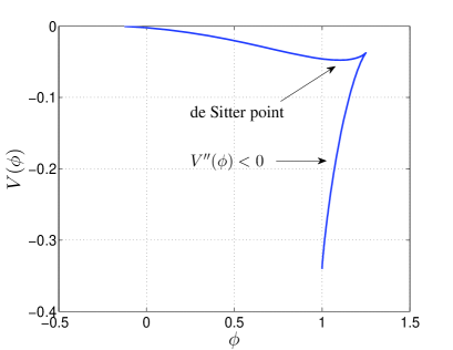
Equation (13) implies that and will change signs at some point, and the potential is folded at that point. When is small, the potential can be folded before reaches the de Sitter point, as shown in Fig. 2. The model is unstable at places where and . When is greater, the folding point of can be shifted to the left side of the de Sitter point, as shown in Fig. 2. Because of the “soft” logarithmic dependence in the function , this model does not have a fully matter-dominated epoch in the early universe.
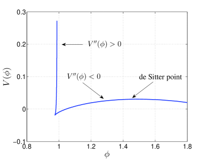
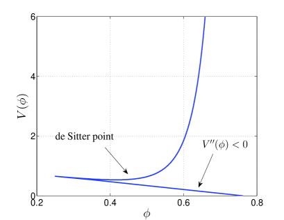
In order to explore other possibilities, one can generalize the function of Eq. (12) as follows:
| (14) |
where is a function of . One may consider a polynomial case as expressed by
| (15) |
When , this model happens to be the simplest format of the Hu-Sawicki model Hu_Sawicki . The complete format of the Hu-Sawicki model is described by Eq. (23). In the case of ,
| (16) |
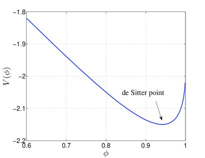
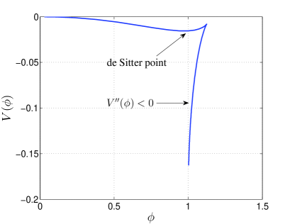
Therefore, will not be zero, and does not have a folding point from the high curvature regime () to the low one (), as is shown in Fig. 4. However, as long as , will include more than one term of with different signs, will have a folding point, and will switch signs at the folding point. As illustrated in Fig. 4, in this case, for some period of from the high to the low curvature regimes, is negative and, consequently, the scalaron is tachyonic. We also considered the exponential case
| (17) |
This model has a similar problem as shown in Fig. 5.
In this class of models of Eq. (14), there are functions of in both the numerator and the denominator of the modification term, which results in having a folding point. At that folding point, switches signs, and the scalaron is tachyonic at places where . To avoid this problem, one may replace the function of in the numerator with a constant, and obtain CDM-like models. In these models, the function is approximately equal to at high curvature, and the modification term will be the decisive term in the late universe.
IV Construction of CDM-like models
IV.1 Procedures
In this study, we construct three types of CDM-like models as expressed by Eqs. (20), (27), and (34), respectively. For simplicity, we take the Type II gravity described by Eq. (27) as an example to explain how to construct viable CDM-like models. The function for the Type II gravity is
| (18) |
The procedures are as follows.
-
1.
The parameters and have the same energy scale as the cosmological constant. For simplicity, is set to be equal to 1.
-
2.
Generally, goes to zero at high curvature, such that the model reduces to the CDM model at high curvature. This will make the model have a matter domination epoch in the early universe, and avoid the solar system tests as well.
-
3.
At high curvature, should be positive to avoid anti-gravity. This can be guaranteed without difficulty, because at high curvature regime the modification term is much less than the main term in the function .
-
4.
The should be positive when , such that the Dolgov-Kawasaki instability can be avoided Dolgov and the scalaron is non-tachyonic. The potential should have a minimum, such that the model is stable and can mimic the later cosmic acceleration. These can be obtained by the following measures.
-
(a)
Note that in theory
(19) Generally, and for the CDM-like models. Therefore, is mainly determined by , and is determined by the modification term in the function . Thus we make sure that and by tuning the sign before .
-
(b)
Let at high curvature. This can be trivially satisfied for a CDM-like model for which and at high curvature.
-
(c)
Tune the parameters and to make sure that as .
-
(a)
-
5.
The requirement of will be consequently satisfied for the CDM-like models once the requirement of is met.
IV.2 Type I CDM-like models
One obtains the first type of CDM-like model by replacing the term in the numerator of the modification term in Eq. (14) with the parameter , so that
| (20) |
where is another parameter. One can construct some viable models as follows by letting take some elementary functions and implementing the procedures discussed in Sec. IV.1.
• Logarithmic format 1:
| (21) |
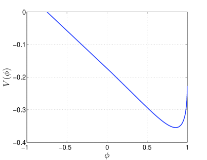
Example parameters for this model are and . The potential for this model with these parameters is plotted in Fig. 6. As expected, the potential has a minimum, and is positive from the high (, ) to the low (, ) curvature regimes. Therefore, this model should be stable, and should also have a sensible cosmological evolution as verified in Sec. V. The potentials for all the CDM-like models presented in this paper have been plotted, with the parameters taking appropriate values. They all look similar to Fig. 6 and therefore are not individually shown here.
• Logarithmic format 2:
| (22) |
For this model, example parameters, which can generate a potential similar to the one plotted in Fig. 6, are and .
• Polynomial format:
| (23) |
where is a positive integer number. Example parameters for this model are , , and . This is the Hu-Sawicki model Hu_Sawicki .
• Exponential format 1:
| (24) |
Example parameters for this model are and . This model is almost the same as the one discussed in Ref. Oikonomou :
| (25) |
where and are parameters.
• Exponential format 2:
| (26) |
Example parameters for this model are , and .
IV.3 Type II CDM-like models
In the Type I models described by Eq. (20), the modification term, , is always finite. Therefore, we can move it to the numerator with the sign before switched, so that
| (27) |
Some models of this type can be constructed as follows.
• Logarithmic format 1:
| (28) |
Example parameters for this model are . When is equal to zero, one obtains
| (29) |
where is a positive parameter. This model is discussed in Ref. Miranda . The model in Eq. (28) reduces to the CDM model faster than the one in Eq. (29).
• Logarithmic format 2:
| (30) |
Example parameters for this model are and .
• Polynomial format:
| (31) |
Example parameters for this model are and . This model and the Hu-Sawicki model in Eq. (23) can be considered to be modifications of the model, in which , where is a parameter with units of mass Carroll . In the model, and are negative, so the scalaron is tachyonic. This problem is avoided in the modified versions in Eqs. (23) and (31).
• Exponential format 1:
| (32) |
Example parameters for this model are and . This model is explored in Refs. Cognola ; Linder ; Bamba ; Elizalde .
• Exponential format 2:
| (33) |
Example parameters for this model are , , and .
IV.4 Type III CDM-like models
One can combine Eqs. (20) and (27), and obtain the third type of CDM-like models
| (34) |
Some models of this type can be constructed as follows.
• Exponential format:
| (35) |
Example parameters for this model are . This model is presented in Ref. Tsujikawa . The model described by Eq. (25) is almost the same as this model.
• Logarithmic format:
| (36) |
Example parameters for this model are and .
• Polynomial format:
| (37) |
Example parameters for this model are , , and .
V Cosmological evolution
In this section, we will explore the cosmological evolution of the CDM-like gravity by taking the model in Eq. (21) as an example.
V.1 Formalism
In this paper, we consider the homogeneous universe in the flat Friedmann-Robertson-Walker metric, . In this case, the universe can be modeled by a four-dimensional dynamical system of , where
| (38) |
is the Hubble parameter, and the dot denotes the derivative with respect to time. Equation (3) provides the dynamical equation for ,
| (39) |
The equation of motion for is
| (40) |
The definition of the Hubble parameter gives
| (41) |
The system is constrained by
| (42) |
where and are the densities of matter and radiation, respectively. Equations (38)-(42) provide a closed description of the dynamical system of .
V.2 The evolution from the exact method
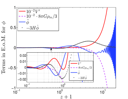
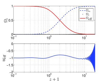
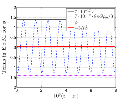
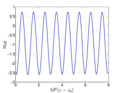
A straightforward way to simulate cosmological evolution is to integrate the equations of motion (39)-(41). However, from the point of view of numerics, at high redshift, the field evolves very slowly and oscillates between and . The behaviors of the terms in Eq. (39) are shown in Fig. 8, revealing the relation between the four terms in Eq. (39): . The field oscillates near the minimum of the effective potential , which is defined by
| (43) |
with
| (44) |
These oscillations produce particles, and could be a possible source of energetic cosmic rays Arbuzova . The oscillations of also make it inconvenient to numerically integrate the evolution in the early universe. Therefore, in the next sub-section, we consider employing an approximation method instead. As a consequence of the oscillations of the field , the equation of state also oscillates near , as shown in Fig. 8.
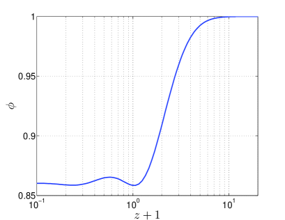
The behaviors of the field and the terms in the equation of motion for (39) at low redshift are shown in Figs. 10 and 10, respectively. Figure 10 reveals that the field has a slow roll when the matter density is greater than the cosmological constant. The field drops significantly as the matter density comes to the cosmological constant scale, oscillates at the minimum of the potential , and then eventually stops due to friction force . As demonstrated in Fig. 10, in the late universe, compared to other terms in Eq. (39), the matter force term is negligible, and Eq. (39) is reduced to
| (45) |
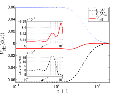
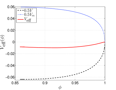
These results can also be interpreted via the effective potential as plotted in Figs. 11 and 12. The effective potential is very flat at high redshift and has a drop at low redshift, such that the field has a slow roll at high redshift and then a drop at low redshift. The evolutions of and at low redshift are shown in Fig. 13. The are defined as , where refers to the indexing of radiation, matter or effective dark energy. The CDM-like models can mimic a cosmological evolution, fitting the observations without difficulty. Comparison of Figs. 8 and 13 demonstrates that the phantom behavior of ( crosses ) at low redshift is nothing but an extension of that behavior at high redshift.
V.3 The evolution from the approximation method
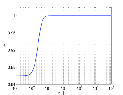
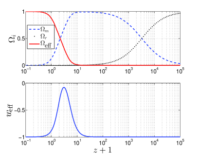
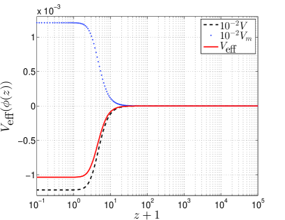
Due to the oscillations of , it is not convenient to numerically integrate the cosmological evolution in the early universe. However, since the field oscillates near the minimum of the effective potential in the early universe, one can take the evolution of the minimum of approximately to be that of the field . The approximate solution describes the evolution of accurately in the early universe. In the late universe, the deviation of the field from the minimum of becomes relatively large, and the exact method should be used as has been done in Sec. V.2.
Equations (38) and (39) can be combined as
| (46) |
For the CDM-like models, the field evolves very slowly in the early universe. From this we get
| (47) |
as shown in Fig. 8. Note that and , where is the matter density of the current universe. These, together with , lead to
| (48) |
Therefore, in our approximation method, we take Eq. (48) as an approximate equation of motion for , we replace Eqs. (38) and (39) by Eq. (48), but keep Eqs. (40)-(42). The results of the approximation method are shown in Figs. 15-16. The field has a slow roll evolution in the early universe due to the approximate balance between and , and the the evolutions of are consistent with cosmological observations.
The exact and the approximate methods are supplementary. The numerical integration in the exact method at high redshift is very slow due to the oscillations of the field , but can mimic the cosmological evolution in the late universe very easily. The approximate method does not yield an accurate cosmological evolution in the late universe, but can mimic a smooth evolution in the early universe. Therefore, these two methods can be used together to explore the cosmic dynamics of gravity.
V.4 The equation of state
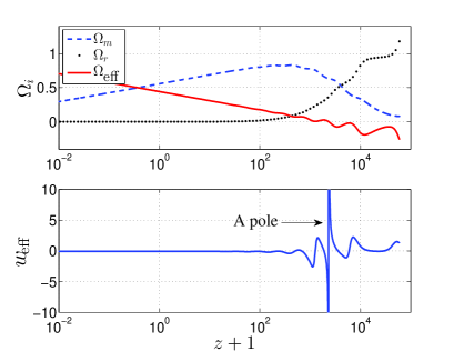
The Big Bang nucleosynthesis and the observations of the Cosmic Microwave Background imply that general relativity should be recovered in the early universe, which means that and as . On the other hand, should be positive to ensure that the scalaron is non-tachyonic. Consequently, should be less than 1 Pogosian . In fact, an greater than 1 in the early universe can cause a pole in the equation of state , as shown in Fig. 17 and also pointed out in Ref. Frolov . This situation can be explained with Eqs. (9) and (10). The first term, , in Eq. (10) can be positive. (This term is equal to and is positive for the model, in which and is positive.) The second term, , is positive because will roll down to the minimum of the potential . However, the third term, , is negative when is greater than 1 in the early universe. Then, in the later evolution, will decrease, cross 1, and move to the minimum of the potential . At some moment, the energy density of the effective dark energy will be zero. This will generate a pole in the equation of state defined by Eq. (9). The CDM-like models do not have such a problem, since the function and in the early universe.
A feasible model should also pass the solar system tests. We studied how the Hu-Sawicki model deals with the solar system tests in Ref. Guo2 . It turned out that the CDM-like models have the advantage of passing the solar system tests.
VI Conclusions
In this paper, we studied how to construct gravity models which satisfy the stability and viability conditions. Cosmological observations and local gravity tests place stringent requirements on the format of the function . A feasible model needs to be very close to the CDM model. For the CDM-like models, it is not hard to obtain the recovery of general relativity in the early universe and a cosmic speed-up in the late universe. The condition can also be easily satisfied since the modification term is usually small compared to the main term in the function . The thing is how to make the potential have a minimum. One way is to tune the parameters, such that , when , and when . Once these have been achieved, the potential will have a minimum. With this method, three types of CDM-like models expressed by Eqs. (20), (27), and (34) are constructed. In addition to these three types, a viable CDM-like may also take other forms. For example, the Starobinsky model takes the form Starobinsky , and a new exponential model takes the form Xu .
We also studied the cosmological evolution of the CDM-like models. The field evolves slowly in the early universe due to the quasi-static balance between and , and is released from the coupling between and in the late universe to generate a dark-energy domination epoch. The numerical simulation is slow in the early universe because of the oscillations of the field near the minimum of the effective potential . To avoid this problem, we take the minimum of as an approximate solution for and obtain the cosmological evolution from the early universe to the late one. This approximation method describes the cosmological evolution well except in the late universe when the curvature scalar is below the cosmological constant scale. We use the exact method to study the late-universe evolution. Then, a combination of the exact and the approximate methods provides a complete picture of the cosmological evolution of gravity.
Acknowledgments
This work was supported by the Discovery Grants program of the Natural Sciences and Engineering Research Council of Canada. The author would like to thank Andrei V. Frolov and Levon Pogosian for useful discussions.
References
- (1) A. G. Riess et al. [ Supernova Search Team Collaboration ], “Observational evidence from supernovae for an accelerating universe and a cosmological constant,” Astron. J. 116, 1009-1038 (1998). [arXiv:astro-ph/9805201]
- (2) S. Perlmutter et al. [ Supernova Cosmology Project Collaboration ], “Measurements of and from 42 high redshift supernovae,” Astrophys. J. 517, 565-586 (1999). [arXiv:astro-ph/9812133]
- (3) A. G. Riess et al. [ Supernova Search Team Collaboration ], “Type Ia supernova discoveries at from the Hubble Space Telescope: Evidence for past deceleration and constraints on dark energy evolution,” Astrophys. J. 607, 665-687 (2004). [arXiv:astro-ph/0402512]
- (4) E. Komatsu et al. [ WMAP Collaboration ], “Seven-year Wilkinson Microwave Anisotropy Probe (WMAP) observations: Cosmological interpretation,” [arXiv:1001.4538 [astro-ph.CO]]
- (5) P. A. R. Ade et al. (Planck Collaboration) “Planck 2013 results. I. Overview of products and scientific results,” arXiv:1303.5062 [astro-ph]
- (6) T. P. Sotiriou and V. Faraoni, “f(R) Theories Of Gravity,” Rev. Mod. Phys. 82, 451-497 (2010). [arXiv:0805.1726v4 [gr-qc]]
- (7) A. D. Felice and S. Tsujikawa, “f (R) Theories,” Living Rev. Rel. 13, 3 (2010). [arXiv:1002.4928 [gr-qc]]
- (8) J. Khoury and A. Weltman, “Chameleon Fields: Awaiting Surprises for Tests of Gravity in Space,” Phys. Rev. Lett. 93, 171104 (2004). [arXiv:astro-ph/0309300v3]
- (9) J. Khoury and A. Weltman, “Chameleon Cosmology,” Phys. Rev. D 69, 044026 (2004). [arXiv:astro-ph/0309411v2]
- (10) I. Navarro and K. V. Acoleyen, “f(R) actions, cosmic acceleration and local tests of gravity,” JCAP 0702, 022 (2007). [arXiv:gr-qc/0611127]
- (11) T. Faulkner, M. Tegmark, E. F. Bunn, and Y. Mao, “Constraining f(R) Gravity as a Scalar Tensor Theory,” Phys. Rev. D 76, 063505 (2007). [arXiv:astro-ph/0612569v1]
- (12) W. Hu and I. Sawicki, “Models of f(R) Cosmic Acceleration that Evade Solar-System Tests,” Phys. Rev. D 76, 064004 (2007). [arXiv:0705.1158v1 [astro-ph]]
- (13) J.-A. Gu and W.-T. Lin, “Solar-System Constraints on f(R) Chameleon Gravity,” arXiv:1108.1782 [gr-qc]
- (14) T. Tamaki and S. Tsujikawa, “Revisiting chameleon gravity - thin-shells and no-shells with appropriate boundary conditions,” Phys. Rev. D 78, 084028 (2008). [arXiv:0808.2284 [gr-qc]]
- (15) S. Tsujikawa, T. Tamaki and R. Tavakol, “Chameleon scalar fields in relativistic gravitational backgrounds,” JCAP 0905, 020 (2009). [arXiv:0901.3226v2 [gr-qc]]
- (16) J.-Q. Guo, “Solar system tests of f(R) gravity,” arXiv:1306.1853 [astro-ph.CO]
- (17) A. D. Dolgov and M. Kawasaki, “Can modified gravity explain accelerated cosmic expansion?” Phys. Lett. B 573, 1 (2003). [arXiv:astro-ph/0307285v2]
- (18) L. Pogosian and A. Silvestri, “The pattern of growth in viable f(R) cosmologies,” Phys. Rev. D 77, 023503 (2008). [arXiv:0709.0296v3 [astro-ph]]
- (19) A. V. Frolov and J.-Q. Guo, “Small Cosmological Constant from Running Gravitational Coupling,” arXiv:1101.4995 [astro-ph.CO]
- (20) J.-Q. Guo and A. V. Frolov, “Cosmological Evolution in f(R) Gravity and a Logarithmic Model,” arXiv:1305.7290 [astro-ph.CO]
- (21) V. K. Oikonomou, “An Exponential F(R) Dark Energy Model,” arXiv:1304.4089 [gr-qc]
- (22) V. Miranda, S. E. Joras, I. Waga, and M. Quartin, “Viable Singularity-Free f(R) Gravity Without a Cosmological Constant,” Phys. Rev. Lett. 102, 221101 (2009). [arXiv:0905.1941v1 [astro-ph.CO]]
- (23) S. M. Carroll, V. Duvvuri, M. Trodden, and M. S. Turner, “Is Cosmic Speed-Up Due to New Gravitational Physics?” Phys. Rev. D 70, 043528 (2004). [arXiv:astro-ph/0306438]
- (24) G. Cognola, E. Elizalde, S. Nojiri, S. D. Odintsov, L. Sebastiani, and S. Zerbini, “Class of viable modified f(R) gravities describing inflation and the onset of accelerated expansion,” Phys. Rev. D 77, 046009 (2008). [arXiv:0712.4017 [hep-th]]
- (25) E. V. Linder, “Exponential Gravity,” Phys. Rev. D 80,123528 (2009). [arXiv:0905.2962 [astro-ph]]
- (26) K. Bamba, C.-Q. Geng, and C.-C. Lee, “Cosmological evolution in exponential gravity,” JCAP 1008, 021 (2010). [arXiv:1005.4574 [astro-ph]]
- (27) E. Elizalde, S. Nojiri, S. D. Odintsov, L. Sebastiani, and S. Zerbini, “Non-singular exponential gravity: a simple theory for early- and late-time accelerated expansion,” Phys. Rev. D 83, 086006 (2011). [arXiv:1012.2280v2 [hep-th]]
- (28) S. Tsujikawa, “Observational signatures of f(R) dark energy models that satisfy cosmological and local gravity constraints,” Phys. Rev. D 77, 023507 (2008). [arXiv:0709.1391 [astro-ph]]
- (29) E. V. Arbuzova, A. D. Dolgova, and L. Reverberid, “Particle Production in f(R) Gravity during Structure Formation,” arXiv:1305.5668 [gr-qc]
- (30) A. A. Starobinsky, “Disappearing cosmological constant in f(R) gravity,” JETP Letter, 86, 157 (2007). [arXiv:0706.2041v2 [astro-ph]]
- (31) Q. Xu and B. Chen “A New Exponential Gravity,” arXiv:1203.6706v3 [astro-ph.CO]