Approximation Schemes for Maximum Weight
Independent Set of Rectangles
Abstract
In the Maximum Weight Independent Set of Rectangles (MWISR) problem we are given a set of axis-parallel rectangles in the 2D-plane, and the goal is to select a maximum weight subset of pairwise non-overlapping rectangles. Due to many applications, e.g. in data mining, map labeling and admission control, the problem has received a lot of attention by various research communities. We present the first -approximation algorithm for the MWISR problem with quasi-polynomial running time . In contrast, the best known polynomial time approximation algorithms for the problem achieve superconstant approximation ratios of (unweighted case) and (weighted case).
Key to our results is a new geometric dynamic program which recursively subdivides the plane into polygons of bounded complexity. We provide the technical tools that are needed to analyze its performance. In particular, we present a method of partitioning the plane into small and simple areas such that the rectangles of an optimal solution are intersected in a very controlled manner. Together with a novel application of the weighted planar graph separator theorem due to Arora et al. [3] this allows us to upper bound our approximation ratio by .
Our dynamic program is very general and we believe that it will be useful for other settings. In particular, we show that, when parametrized properly, it provides a polynomial time -approximation for the special case of the MWISR problem when each rectangle is relatively large in at least one dimension. Key to this analysis is a method to tile the plane in order to approximately describe the topology of these rectangles in an optimal solution. This technique might be a useful insight to design better polynomial time approximation algorithms or even a PTAS for the MWISR problem. In particular, note that our results imply that the MWISR problem is not -hard, unless .
1 Introduction
One of the most fundamental problems in combinatorial optimization is the Independent Set problem: given an undirected graph, find a set of pairwise non-adjacent vertices with maximum total weight. While the general problem is essentially intractable (it is -hard to approximate with a factor for any [20]), many special cases allow much better approximation ratios.
One extensively studied setting are graphs which stem from geometric shapes in the 2D-plane. Given a set of geometric objects in the plane, the goal is to find a set of pairwise non-overlapping objects with maximum total weight. Depending on the complexity of these shapes, the approximation factors of the best known polynomial time algorithms range from for fat objects [10], to for arbitrary shapes [12]. Observe that the latter is still much better than the complexity lower bound of for arbitrary Independent Set instances.
Interestingly, there is a very large gap between the best known approximation factors when the considered objects are squares of arbitrary sizes and when they are rectangles. For squares, a -approximation has been known for several years [10]. For the rectangles, the best known approximation factors are for the general case [8], and for the cardinality case [6]. Importantly, no constant factor approximation algorithms are known for rectangles, while the best known hardness result is -hardness [11, 14]. These gaps remain despite a lot of research on the problem [2, 4, 6, 7, 8, 11, 14, 15, 17, 18], which is particularly motivated by its many applications in areas such as channel admission control [17], map labeling [2, 9], and data mining [13, 15, 16].
Since even for arbitrary shapes the best known hardness result is -hardness, it seems that more sophisticated algorithmic techniques and/or complexity results are needed to fully understand the Independent Set problem in the geometric setting.
1.1 Related Work
The maximum weight independent set of rectangles problem has been widely studied. There are several approximation algorithms known [2, 15, 18], and in fact the hidden constant can be made arbitrarily small since for any there is a -approximation algorithm due to Berman et al. [4]. Eventually, a -approximation algorithm has been presented by Chan and Har-Peled [8]. Some algorithms have been studied which perform better for special cases of MWISR. There is a -approximation algorithm due to Lewin-Eytan, Naor, and Orda [17] where denotes the size of the largest clique in the given instance. In case that the optimal independent set has size for some , Agarwal and Mustafa present an algorithm which computes an independent set of size [1].
In a break-through result, Chalermsook and Chuzhoy give a -approximation algorithm for the cardinality case [6], which is based on the natural LP-relaxation of the problem. In fact, it is a challenging open problem to determine the exact integrality gap of the LP. Currently the best known upper bounds for it are [8] for the weighted case, and [6] for the cardinality case. The best known lower bounds on the integrality gap are [6] and 2 [19], both already for the cardinality case. There is a strong connection between the integrality gap of the LP and the maximum ratio between the coloring- and the clique-number of a set of rectangles, see [5] and references therein.
Interestingly, for the special case when all given rectangles are squares of arbitrary sizes, the problem is much better understood. There is a polynomial time -approximation algorithm by Erlebach, Jansen and Seidel [10], which works even for the more general case of arbitrary fat objects. For the unweighted squares, and also for the more general setting of unweighted pseudo-disks, even a simple local search algorithm gives a PTAS [8].
Although the complexity is well-understood in the setting of squares, for rectangles it is still widely open. In particular, the techniques of the above approximation schemes for squares do not carry over to rectangles. The PTAS from [10] requires that every horizontal or vertical line intersects only a bounded number of objects of the optimal solution that are relatively large in at least one dimension. For rectangles, this number can be up to which is too much. For local search, one can easily construct examples showing that for any size of the local search neighborhood (which gives quasi-polynomial running time) the optimum is missed by an arbitrarily large (superconstant) factor.
For arbitrary shapes in the plane (which can be modeled as a set of line segments) Agarwal and Mustafa [1] give an algorithm which finds an independent set of size which yields a worst case approximation factor of . This was improved by Fox and Pach to for any [12]. Note that already for lines with at most one bend (i.e., lines forming an “L”) the natural LP-relaxation suffers from an integrality gap of .
To the best of our knowledge, no inapproximability result is known for MWISR (and not even for arbitrary shapes in the 2D-plane). In particular, an important open problem is to construct a polynomial time constant factor approximation algorithm for MWISR.
1.2 Our Contribution and Techniques
We present the first -approximation algorithm for the Maximum Weight Independent Set of Rectangles problem with a quasi-polynomial running time of . In contrast, the best known polynomial time approximation algorithms achieve approximation ratios of for the weighted case [8], and for the cardinality case [6]. We are not aware of any previous algorithms for the problem with quasi-polynomial running time which would give better bounds than the above mentioned polynomial time algorithms. Our quasi-PTAS rules out the possibility that the problem is -hard, assuming that , and thus it suggests that it should be possible to obtain significantly better polynomial time approximation algorithms for the problem. In addition, we present a PTAS for the case that each rectangle is -large in at least one dimension, i.e., if at least one of its edges has length at least for some constant , assuming that in the input only integer coordinates within occur.
Key to our results is a new geometric dynamic program GEO-DP whose DP-table has one entry for each axis-parallel polygon with at most edges, where is a fixed parameter. Such a cell corresponds to a subproblem where the input consists only of the input rectangles contained in . The algorithm solves each such subproblem by trying every possible subdivision of into at most polygons with again at most edges each, and selects the partition with maximum weight according to the DP-cells of all subproblems.
For analyzing this algorithm, we show that there is a recursive sequence of partitions such that the rectangles of intersected within that sequence have a total weight of at most . For our QPTAS, we first provide a method to tile the plane into polygons such that each rectangle of the optimal solution is intersected only times. Using a new stretching method for the input area, we can guarantee that each face of our partition either contains only rectangles of relatively small total weight, or contains at most one rectangle. With a planar separator theorem from [3] we can find a cut in the partition such that the intersected rectangles have only marginal weight and both sides of the cut contain rectangles whose total weight is upper bounded by . When using these cuts in every iteration, the recursion terminates after levels and we show that by setting we obtain an approximation ratio of in quasi-polynomial time.
We demonstrate the potential of our new algorithm by proving that it yields a polynomial time -approximation algorithm for the special case when each rectangle is large in at least one dimension, as defined above. For this result, we employ a finer partition of the plane which ensures that in the initial partition only large rectangles with small total weight are intersected. Even more, each face of the subdivision is either a path or a cycle of a small width (strictly smaller than the longer edge of each large rectangle). Using this, we show that GEO-DP solves each resulting subproblem within an accuracy of by using only subpolygons with at most a constant number of edges. Therefore, we prove that GEO-DP parametrized by gives a polynomial time -approximation for -large rectangles (for any constant ). In fact, this yields a PTAS for the case that the lengths of the longer edges of the rectangles differ by at most a constant factor (when the parameter is chosen appropriately). We would like to point out that the initial partition might be a useful ingredient for constructing a PTAS for the general problem since it sparsely describes the topology of the large rectangles while losing only an -fraction of their total weight.
We can well imagine that our algorithmic approach finds applications for solving the Independent Set problem for more general geometric shapes. Given the large gaps in terms of approximation and hardness results for the Independent Set problem in such settings we hope that our new techniques will help to bridge these gaps. Finally, we would like to note that our DP might well yield a constant factor approximation or even a PTAS for MWISR when parametrized by a sufficiently large parameter independent of , e.g., . We leave this as an open question.
1.3 Problem Definition
We are given a set of axis-parallel rectangles in the -dimensional plane. Each rectangle is specified by two opposite corners and , with and , and a weight . We define the area of a rectangle as the open set . The goal is to select a subset of rectangles such that for any two rectangles we have . Our objective is to maximize the total weight of the selected rectangles . For each rectangle we define its width by and its height by .
By losing at most a (multiplicative) factor of in the objective, we assume that for each rectangle . First, we scale the weights of all rectangles such that . Since then , all rectangles with can contribute a total weight of at most . We remove them from the instance which reduces the weight of the optimal solution by at most .
2 The Algorithm GEO-DP
Our results are achieved by using a new geometric dynamic programming algorithm which we call GEO-DP and which we define in this section. The algorithm is parametrized by a value which affects both the running time and the achieved approximation ratio. In brief, the algorithm has a DP-cell for each axis-parallel polygon with at most edges, which represents the subproblem consisting of all rectangles contained in . When computing a (near-optimal) solution for this subproblem, GEO-DP tries all possibilities to subdivide into at most polygons with at most edges each and recurses.
Without loss of generality we assume that for each . If this is not the case, we transform the instance in polynomial time into a combinatorially equivalent instance with the latter property.
Fix a parameter . Let denote the set of all polygons within the input square whose corners have only integer coordinates and which have at most axis-parallel edges each. Whenever we speak of a polygon, we allow it to have holes and we do not require it to be simple. In particular, by the edges of a polygon with holes we mean both the outer edges and the edges bounding the holes. We introduce a DP-cell for each polygon , where a cell corresponding to stores a near-optimal solution where denotes the set of all rectangles from which are contained in .
Proposition 1.
The number of DP-cells is at most .
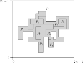
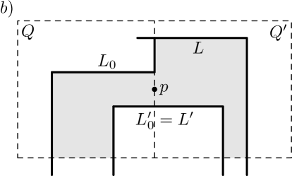
To compute the solution for some polygon we use the following procedure. If then we set and terminate. Otherwise, we enumerate all possibilities to partition into polygons such that . See Figure 1 for a sketch. Since by Proposition 1 we have , the number of potential partitions we need to consider is upper bounded by . Let , where , be a feasible partition (for any enumerated set this can be verified efficiently since all polygons have axis-parallel edges with integer coordinates in ). For each polygon we look up the DP-table value and compute . We set for the partition which yields the maximum profit. Now we define if , and otherwise for a rectangle with maximum profit. At the end, the algorithm outputs the value in the DP-cell which corresponds to the polygon containing the entire input region .
Since we get the following upper bound on the running time of GEO-DP.
Proposition 2.
When parametrized by the running time of GEO-DP is upper bounded by .
For bounding the approximation ratio of GEO-DP for any parameter , it is sufficient to consider only the special case that the input set is already a feasible (optimal) solution. Therefore, we will assume this from now on.
3 Quasi-Polynomial Time Approximation Scheme
In this section we prove that GEO-DP achieves an approximation ratio of when parametrized by and is thus a QPTAS for the MWISR problem (using Proposition 2).
Key ingredient for our analysis is to show that for any set of feasible rectangles there is a balanced cheap cut, i.e., a polygon which consists of only few edges, which intersects rectangles from of marginal total weight, and which separates the rectangles from into two parts of similar size. By applying such cuts recursively for levels, we eventually obtain trivial subproblems. For proving that such good cuts always exist, we partition the plane into polygons in such a way that each rectangle is intersected only times and each face of the partition consists either of exactly one rectangle or intersects rectangles of only small total weight. To ensure the latter, we apply a stretching procedure to the input before actually defining the partition. On the constructed partition we apply the weighted planar graph separator theorem from [3] to obtain the cut.
3.1 Balanced Cheap Cuts
We introduce balanced -cheap -cuts, where is a small positive value. Intuitively, given any set of non-overlapping rectangles , such a cut is given by a polygon with at most axis-parallel edges whose boundary intersects rectangles with weight at most such that the interior and the exterior of each contain only rectangles whose weight is at most .
Definition 3.
Let and with . Let be a set of pairwise non-overlapping rectangles. A polygon with axis-parallel edges is a balanced -cheap -cut if:
-
•
has at most edges,
-
•
for the set of all rectangles intersecting the boundary of we have ,
-
•
for the set of all rectangles contained in it holds that , and
-
•
for the set of all rectangles contained in the complement of , i.e., in , it holds that .
As we will show in the next lemma, GEO-DP performs well if for any set of rectangles there exists a good cut.
Lemma 4.
Let . Let with and be values such that for any set of pairwise non-overlapping rectangles there exists a balanced -cheap -cut, or there is a rectangle such that . Then GEO-DP has approximation ratio when parametrized by .
Proof (sketch). .
Starting with the input square, we either find a rectangle with , or a balanced -cheap -cut. In either case we get a decomposition of the problem into subproblems, where each subproblem is defined by a polygon which contains rectangles whose total weight is at most a -fraction of . Continuing for recursion levels, we obtain subproblems consisting of at most one rectangle each (as for each ). Each appearing subproblem can be expressed as the intersection of polygons with at most edges each (we have to add since the boundary of the input square can become the outer boundary of a polygon). Thus, the boundary of each considered subproblem consists of edges. Additionally, we can show that each subproblem gives rise to subproblems in the next recursion level. As GEO-DP tries all partitions of a polygon into at most polygons, each with at most edges, at each recursion level it will consider the partition corresponding to the cut. Since at each level we lose rectangles whose weight is at most an -fraction of the total weight of the rectangles from the current recursion level, we obtain the claimed approximation ratio. ∎
In the remainder of this section we prove that for any set and any there is a balanced -cheap -cut or there is a rectangle with . This implies our main result when choosing . Note that from now on our reasoning does not need to be (algorithmically) constructive.
3.2 Stretching the Rectangles
For the purpose of finding a good cut, we are free to stretch or squeeze the rectangles of . We do this as a preprocessing step in order to make them well-distributed.
Definition 5.
A set of rectangles with integer coordinates in is well-distributed if for any and for any we have that all rectangles contained in the area have a total weight of at most . We require the same for the rectangles contained in the area .
We say that two sets of rectangles are combinatorially equivalent if we can obtain one from the other by stretching or squeezing the input area, possibly non-uniformly (see Appendix B for a formal definition).
Lemma 6.
Let be a set of rectangles with arbitrary weights. There is a combinatorially equivalent set using only integer coordinates in which is well-distributed.
Proof (sketch). .
Without loss of generality we assume that for each , where . We stretch the original input square in such a way that the lengths of its sides double (i.e., increase by another ), and the distance between two original consecutive -coordinates (-coordinates) and increases proportionally to the weight of all rectangles "starting" at the -coordinate (-coordinate) . We then need to introduce some rounding, as we want the new coordinates of all the rectangles to be integral. The new set of rectangles is clearly equivalent to the original one.
Consider any vertical stripe in the modified input square with left- and rightmost -coordinates and , respectively. There is a set of -coordinates from the original instance which were mapped to values . All rectangles contained in must have their respective leftmost -coordinates in . The total weight of rectangles with leftmost coordinate is proportional to , for each . Hence, the total weight of rectangles contained in is proportional to . The same is true for horizontal stripes, and so the modified input instance is well-distributed. ∎
Observe that there is a balanced -cheap -cut for any values and in the stretched instance if and only if there is such a cut in the original instance. Thus, suppose from now on that we have a well-distributed set of pairwise non-intersecting rectangles , using integer coordinates in for some integer , and a value such that . As we do not require any special bound on the value of , we can scale up all coordinates of the rectangles by a factor of , and therefore we can assume that is an integer.
3.3 Partitioning the Plane
We define a procedure to partition the input square . This partition is defined by only lines, and it has the properties that each rectangle in is intersected only times and each face either surrounds exactly one rectangle or it has non-empty intersection with rectangles with small total weight of at most .
We call a rectangle large if or , and small if and . We denote the subsets of consisting of large and small rectangles by and , respectively. We call a rectangle vertical if , and horizontal if . We say that a line cuts a rectangle , if has two connected components.
We now present the construction of the partition. It will consist of a set of straight axis-parallel lines contained in the input square , and containing the boundary of . A connected component of is called a face, and the set of faces is denoted by . Note that the faces are open polygons and for any and we have .
Grid.
We subdivide the input square into grid cells, where each grid cell is a square of size . Formally, for each we have a grid cell . As is an integer, the corners of the grid cells have integer coordinates. The lines subdividing the input square into the grid cells are called grid lines.
We say that a rectangle intersects a grid cell , if (recall that rectangles have been defined as open sets). Each rectangle intersects at least two grid cells, and each rectangle intersects at most four grid cells. We say that a rectangle crosses a grid cell , if intersects and has non-empty intersection with two opposite edges of . Notice that small rectangles do not cross any grid cells.
Rectangle faces.
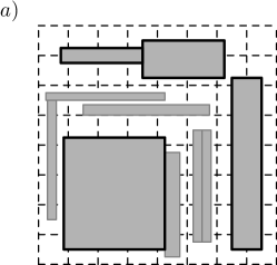
For each large vertical rectangle which is cut by a vertical grid line, and for each large horizontal rectangle which is cut by a horizontal grid line, we add the edges of the rectangle to the set of lines (see Figure 2a). The added edges are called rectangle edges, and the faces corresponding to such rectangles are called rectangle faces.
Lemma 7.
The number of rectangle faces is at most .
Notice that if a large vertical rectangle is not contained in a rectangle face then it is contained in a single column of grid cells. Similarly, if a large horizontal rectangle is not contained in a rectangle face then it is contained in a single row of grid cells.
Lines within the grid cells.
We now consider each grid cell separately, and proceed as follows. Let denote the set of rectangles from which are not contained in the rectangle faces, and which cross . Notice that, as the rectangles from are pairwise non-overlapping, cannot contain both vertical and horizontal rectangles.
-
•
If , we add to the whole boundary of , with the exception of the fragments which are in the interior of the rectangle faces (see Figure 3a).
Notice that the boundaries of the rectangle faces are in , so in this case is connected.
-
•
If consists of vertical rectangles, let and be the leftmost and the rightmost vertical edge of a rectangle from . We add to the lines and , and the boundary of with the exception of the fragments which are between and , or in the interior of the rectangle faces (see Figure 3b).
Notice that the lines added to while considering the grid cell do not intersect any rectangles from .
-
•
If consists of horizontal rectangles, we proceed as before, considering horizontal lines instead of vertical (see Figure 3c).

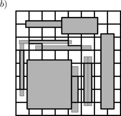
Notice that the lines from can overlap (i.e., we can have s.t. is an interval), but they do not intersect properly (i.e., if for we have , then is an endpoint of at least one of the lines ). The lines from cover the boundary of the input square . An example of the partition can be seen in Figure 2b.
Graph .
We now construct a graph embedded in the input square , representing the partition . Any point becomes a vertex of if and only if there is at least one line with an endpoint in . For any pair of vertices for which there is a line such that , and for which no vertex lies on the straight line strictly between and , we add an edge to (i.e., edges of represent subdivisions of lines in ). As , the faces of are exactly . The claim of the next lemma is directly implied by the construction.
Lemma 8.
The graph is planar and has vertices and edges.
The following lemmas will be needed to show the existence of a balanced cut in .
Lemma 9.
Each rectangle from can be intersected by at most four edges of the graph .
Proof (sketch). .
The only edges of intersecting rectangles from lie on grid cell boundaries. We can show that any rectangle can be intersected by at most one edge of at each grid cell boundary.
As any intersects at most four grid cell boundaries, the lemma holds for small rectangles. The lemma clearly holds for any rectangle contained in a rectangle face. The remaining case are large rectangles contained in a single row or column of grid cells. From the construction of for single grid cells we can show that such a rectangle can be intersected only at the two extremal grid cell boundaries within . ∎
Lemma 10.
Let . The boundary of intersects rectangles from of total weight at most . If is not a rectangle face, then has non-empty intersection with rectangles from of total weight at most .
Proof (sketch). .
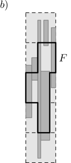
The lemma clearly holds for rectangle faces. Let be face which is not a rectangle face. If is contained in one grid cell then one can show that all rectangles intersecting must be contained in the area defined by grid column and grid row containing together with the two adjacent grid rows (see Figure 7a). On the other hand, if spans several grid cells, one can show that all rectangles intersecting it must be contained in a single grid row or column (see Figure 7b). In both cases, the claim follows since is well-distributed. ∎
3.4 Defining the Cut
For obtaining our desired cut, we apply the following theorem from [3] for the graph . A V-cycle is a Jordan curve in the embedding of a given planar graph which might go along the edges of and also might cross faces of . The parts of crossing an entire face of are called face edges.
Theorem 11 ([3]).
Let denote a planar, embedded graph with weights on the vertices and faces and with costs on the edges. Let denote the total weight, and the total cost of the graph. Then, for any parameter , we can find in polynomial time a separating V-cycle such that
-
•
the interior and exterior of each has weight at most ,
-
•
uses at most face edges, and
-
•
uses ordinary edges of total cost .
First, we need to assign costs to the edges of and weights to the vertices and faces of . For each edge we define its cost to be the total weight of rectangles intersecting . The weights of all vertices are zero. For each face we define its weight to be the total weight of all rectangles contained in , plus a fraction of the weight of the rectangles which intersect the boundary of . If a rectangle has non-empty intersection with faces, each of these faces obtains a -fraction of the weight of . From Lemmas 9 and 10 we obtain the following bounds.
Lemma 12.
The total cost of edges in is at most . The weight of each non-rectangle face is at most . The total weight of the faces equals .
For constructing the cut we apply Theorem 11 with parameter to the graph . The obtained V-cycle yields a cut in the plane. We replace each face edge crossing some face by the edges going along the boundary of . If for each rectangle and if , then, from Lemma 10, each face has weight at most . We can then ensure that each side of the modified cut contains rectangles of total weight at most . Using the upper bound on the number of edges of from Lemma 8, and upper bounding the total weight of rectangles intersected by the modified cut (using Lemmas 10 and 12) implies the following result.
Lemma 13.
Assume that . For any set of pairwise non-overlapping rectangles not containing a rectangle of weight at least there exists a balanced -cheap -cut.
Theorem 14.
The algorithm GEO-DP parametrized by yields a quasi-polynomial time approximation scheme for the maximum weight independent set of rectangles problem.
4 A PTAS for Large Rectangles
In this section we show that GEO-DP yields a polynomial time approximation scheme for input instances which contain only large rectangles, i.e., in which every rectangle has width or height greater than a -fraction of the length of the edges of the input square, for some constant . As a corollary, we obtain a PTAS for the special case of the MWISR problem when the lengths of the longer edges the rectangles differ only by a constant factor, i.e., for some constant we have for all rectangles .
Let and . Let be a set of rectangles, and let be an integer such that for each rectangle we have . We call a rectangle -large if or . In this section we assume that the input consists of a set of -large rectangles for some constant . Assume w.l.o.g. that and . As in the previous section, for the analysis of GEO-DP we can assume that itself is the optimal solution, i.e., no two rectangles in overlap.
Overview.
First, we show that there is a way to partition the plane using a set of at most lines, such that the intersected rectangles have small total weight and each face of the partition is a path or a cycle of “width” at most . Note that the latter bound is strictly smaller than the length of the longer edge of each rectangle. In a sense, this partition sparsely describes the topology of the (large) rectangles while losing only rectangles of negligible weight. Then, we show that for each face GEO-DP can solve the resulting subproblem within a -accuracy, without an increase in the complexity of the subproblems during the recursion.
When given an input instance, GEO-DP first preprocesses it so that all rectangles have coordinates which are integers in . Note, however, that this routine might cause that some rectangles are not -large anymore. Therefore, in the analysis in this section, we show that a good recursive subdivision of the input square exists for the original input with coordinates in for some integer , and where all the rectangles are -large. As the preprocessing consists essentially of stretching and squeezing of the input area, there is a corresponding recursive subdivision of the preprocessed input instance, whose polygons have the same complexity, and which will be considered by GEO-DP. W.l.o.g. we assume that is an integer.
4.1 Constructing the Partition for Large Rectangles
We define a set of lines forming a partition in the input square . The lines in will have the properties that
-
•
,
-
•
the rectangles intersected by a line in have a total weight of at most , and
-
•
each face in the partition obtained by which contains rectangles from is either a path or a cycle with “width” at most .
Without saying explicitly, from now on each considered line is either horizontal or vertical and its endpoints have integral coordinates.
Grid and blocks.
We construct a grid consisting of grid cells in the input square , i.e., for each there is a grid cell with coordinates .
We slice all rectangles parallel to their longer edge into blocks, i.e., rectangles of unit width or height. Formally, we cut each rectangle with into vertical blocks, with the corners and for . With a symmetric operation we generate horizontal blocks for each rectangle with . We denote by the set of all generated blocks and observe that also they have integer coordinates. Like the rectangles, we define the blocks as open sets. We will first find a partition for the blocks, which essentially means that in the first version of the partition we can cut the rectangles arbitrarily parallel to their longer edges. Later we will show how to adjust the partition—by introducing some detours—so that these cuts will be eliminated.
We use the following notation. A line touches a rectangle if . A line intersects a rectangle if . A line hits a rectangle if touches , does not intersect , but extending would result in intersecting . A line cuts a rectangle if has two connected components. We say that a rectangle (a block , a line ) intersects a grid cell if (, ). Each rectangle , as well as each block , intersects at least two grid cells. We say that a block ends in a grid cell , if intersects , and for a short edge (i.e., an edge with unit length) of we have .
Initial set of lines.
We start by introducing an initial set of lines as follows. First, we add to four lines which form the boundary of the input square .
Consider a grid cell and its bottom edge . If possible, we add to the following maximal lines which do not intersect any block or any line previously added to , which touch , and which are strictly longer than :
-
•
a vertical line with the smallest possible -coordinate,
-
•
a vertical line with the largest possible -coordinate,
-
•
a vertical line which maximizes the length of . If there are several such lines, we add two: one with the smallest and one with the largest -coordinate. Lines maximizing are called sticking-in lines for in . The ones added to in this step are called extremal sticking-in lines.
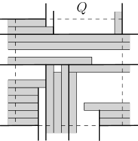
We do the same operation for the top, left and right edges of , where for the left and right edges we take horizontal lines, considering the -coordinates instead of the -coordinates. We do this in a fixed order, e.g., first we add all vertical lines, and then all horizontal lines. See Figure 4 for an example. We do not want to be a multi-set and thus we add each line at most once. Note that for any two lines the intersection is either empty or consists of one single point (which is the endpoint of one of the lines). All lines in are maximal, which means that they cannot be extended without intersecting any perpendicular block or a perpendicular line in .
Proposition 15.
The set consists of at most lines.
Extending lines.
A line in might have loose ends which are endpoints which are not contained in some other line in . We fix this by adding a set of lines . We extend each loose end of a line in by a path connecting either to a line in or to a line in the so far computed set . Such a path will contain horizontal or vertical line segments, and will cut only rectangles of total weight parallel to their shorter edges. We add the lines of this path to and continue with the next loose end of a line in .
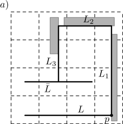
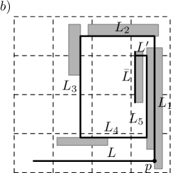
The details of the construction can be found in Appendix C. Here we present just the idea of the construction. As all lines from are maximal, if an endpoint of a line does not hit a line from then it must hit a perpendicular block . The first line on the path goes along the boundary of such that it crosses the boundary of a grid cell (as blocks are not contained in a single grid cell, their longer edges always cross the boundary of a grid cell). We extend so that it either touches a line from (and the construction of the path is finished), or hits some perpendicular block. In the latter case we proceed with the construction of the path, considering a loose end of instead of . Notice that in this part of the construction the path does not intersect any rectangles parallel to their shorter edges (i.e., it does not intersect any blocks). After steps either the path ends by touching a line from , or we can make a shortcut by adding a line at the end of the path such that goes along a grid cell boundary, connects the path with a line from , and cuts rectangles of total weight parallel to their shorter edges. See Figure 5 for an example of the construction.
We say that a set of lines is nicely connected if no two lines overlap (i.e., share more than one point) or intersect properly (i.e., such that has four connected components) and for any endpoint of a line there is a line , perpendicular to , such that .
Lemma 16.
The set of lines is nicely connected, , and the total weight of rectangles in cut by some line in parallel to their shorter edge is upper bounded by . Also, all lines in cutting rectangles in lie on some grid line and for each line there exists no cell such that .
Faces of the partition.
The lines subdivide the input square into a set of faces which are the connected components of (so in particular, the faces are open sets). Denote by the set of all faces of this partition, and by the set of all faces which contain at least one block from . As the next lemma shows, inside of each grid cell each face from the set has a simple structure. We say that a polygon is an L-shape if its boundary has exactly six axis-parallel edges.
Lemma 17.
Consider a face and let be a grid cell with . Consider one connected component of . Then is the interior of a rectangle or the interior of an L-shape. Also, consists of one or two disjoint lines, where denotes the boundary of .
Proof (sketch)..
First, assume that there is an edge of and two lines from the boundary of such that and the subsegment of between and is contained in . Using that the extremal sticking-in lines of belong to , with some careful analysis we can show that there is an edge of and two lines connecting and with , respectively (possibly and ). With this insight and the fact that the lines in are nicely connected, we can show that if is opposite of then is the interior of a rectangle, otherwise is the interior of an L-shape.
Next, we need to show that an edge and lines with the needed properties always exist. First, we show that they exist if has a non-empty intersection with some block contained in . That holds, as for some edge of we have and then . As the extremal long lines crossing are in , there are lines with the properties above which “surround” within , and they form the boundary of . Last, we show that if we have two neighboring connected components and and the needed properties hold for one of them, then they must hold for the other one as well. ∎
Now we study the structure of the faces in at the boundary of the grid cells. In the following lemma we show that multiple connected components of a face inside one grid cell cannot merge into one component in a neighboring grid cell .
Lemma 18.
Let and be grid cells such that for an edge . Consider a face such that , and let be a connected component of such that . Then there is exactly one connected component of such that .
Proof (sketch)..
Clearly, at least one such component exists since . Assume for contradiction that there are two connected components and of with non-empty intersection with . Then there must be a line intersecting which touches between and . We can show, from the construction of the lines in , that is connected with a boundary of in via a line from . This is a contradiction, as then either or does not intersect . ∎
Circumventing some rectangles.
As the last step of the construction of the partition, we want to ensure that if a line in our construction intersects a rectangle , then it cuts parallel to its short edge. We achieve this as follows: whenever a line intersects a rectangle such that has only one connected component or is longer than , then we add the four edges of as new lines and remove all parts of lines from which are inside . For any line in this operation adds at most new lines. Denote by the resulting final set of lines. Similarly as above, the set denotes all faces, and the set denotes all faces which contain at least one rectangle.
Using the bounds on the number of edges in from Proposition 15 and Lemma 16, and the upper bound on the total weight of rectangles in cut by a line from parallel to its shorter edge (Lemma 16), we can show the following result.
Lemma 19.
The set of lines has the properties that and the total weight of intersected rectangles is upper bounded by .
4.2 Solving the Subproblems for the Faces
We transform the set of lines into a graph in the same way as in Section 3. From Lemma 19 we get that and . The algorithm GEO-DP parametrized with tries to subdivide the input square into the faces and then recurses on the subproblems given by the faces. Observe that each face in does not contain any rectangle from and thus we ignore those faces from now on. We distinguish two types of faces in : faces which are homeomorphic to a straight line, and those homeomorphic to a cycle. Note that due to Lemma 17 and Lemma 18 no more complex shapes can arise.
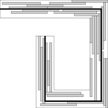
Let be homeomorphic to a straight line. We claim that GEO-DP finds an optimal solution for . To get some intuition, let us pretend that is the union of a set of complete grid cells and that all rectangles inside are blocks, i.e., or for each with . Then there exists a cut through which splits into two sub-faces without intersecting any rectangle (see Figure 6a). Moreover, the boundary of each sub-face will not be more complex than the boundary of itself. Due to this, the complexity of the subproblems does not increase during the recursion process, and the algorithm GEO-DP finds an optimal solution for . While for arbitrary faces homeomorphic to a straight line and arbitrary rectangles instead of blocks the analysis is more technical, and in particular requires circumventing rectangles within , the key concept is the same.
Lemma 20.
Consider a face which is homeomorphic to a straight line. Then GEO-DP parametrized by a value computes an optimal solution for the DP-cell corresponding to .
 |
 |
|
| (a) | (b) |
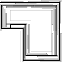
Now consider a face which forms a cycle, i.e., which is homeomorphic to . Let us pretend again that is the union of some complete grid cells and all rectangles in are blocks. Then we can split into a path-face and a smaller cycle while ensuring that the boundary of the faces and consists of at most edges each (see Figure 6b). The recursion terminates when at some recursion level . When doing this operation repeatedly, we ensure that the total weight of intersected rectangles is only an -fraction of the total weight of the rectangles in the paths that we detached from the cycle.
Using this construction we can show that GEO-DP parametrized by sufficiently large computes a -approximation for , using that it solves the subproblems for path-faces optimally. Again, for arbitrary rectangles and more general cycle-faces the reasoning is more technical while the core idea stays the same.
Lemma 21.
Consider a face which is homeomorphic to . Then GEO-DP parametrized by a value computes a -approximative solution for the DP-cell corresponding to .
When constructing the partition given by the lines we intersect (and thus lose) rectangles of total weight at most . When solving the subproblems given by the faces of the partition we again lose rectangles of total weight at most . Thus, by choosing , GEO-DP yields a PTAS.
Theorem 22.
Let and be constants.
Using standard shifting technique arguments we obtain the following corollary.
Corollary 23.
Let and be constants. The algorithm GEO-DP parametrized by is a polynomial time -approximation algorithm for instances of MWISR where for all rectangles it holds that .
References
- [1] P. K. Agarwal and N. H. Mustafa. Independent set of intersection graphs of convex objects in 2d. Computational Geometry, 34(2):83–95, 2006.
- [2] P. K. Agarwal, M. van Kreveld, and S. Suri. Label placement by maximum independent set in rectangles. Computational Geometry, 11:209 – 218, 1998.
- [3] S. Arora, M. Grigni, D. Karger, P. Klein, and A. Woloszyn. A polynomial-time approximation scheme for weighted planar graph tsp. In Proceedings of the ninth annual ACM-SIAM symposium on Discrete algorithms, SODA ’98, pages 33–41, Philadelphia, PA, USA, 1998. Society for Industrial and Applied Mathematics.
- [4] P. Berman, B. DasGupta, S. Muthukrishnan, and S. Ramaswami. Improved approximation algorithms for rectangle tiling and packing. In Proceedings of the twelfth annual ACM-SIAM symposium on Discrete algorithms, pages 427–436. Society for Industrial and Applied Mathematics, 2001.
- [5] P. Chalermsook. Coloring and maximum independent set of rectangles. Approximation, Randomization, and Combinatorial Optimization. Algorithms and Techniques, pages 123–134, 2011.
- [6] P. Chalermsook and J. Chuzhoy. Maximum independent set of rectangles. In Proceedings of the 20th Annual ACM-SIAM Symposium on Discrete Algorithms (SODA ’09), pages 892–901. SIAM, 2009.
- [7] T. M. Chan. A note on maximum independent sets in rectangle intersection graphs. Information Processing Letters, 89(1):19–23, 2004.
- [8] T. M. Chan and S. Har-Peled. Approximation algorithms for maximum independent set of pseudo-disks. In Proceedings of the 25th annual symposium on Computational geometry, SCG ’09, pages 333–340, New York, NY, USA, 2009. ACM.
- [9] J. S. Doerschler and H. Freeman. A rule-based system for dense-map name placement. Communications of the ACM, 35(1):68–79, 1992.
- [10] T. Erlebach, K. Jansen, and E. Seidel. Polynomial-time approximation schemes for geometric graphs. In Proceedings of the 12th Annual ACM-SIAM Symposium on Discrete Algorithms (SODA ’01), pages 671–679. SIAM, 2001.
- [11] R. J. Fowler, M. S. Paterson, and S. L. Tanimoto. Optimal packing and covering in the plane are np-complete. Information processing letters, 12(3):133–137, 1981.
- [12] J. Fox and J. Pach. Computing the independence number of intersection graphs. In Proceedings of the Twenty-Second Annual ACM-SIAM Symposium on Discrete Algorithms, SODA ’11, pages 1161–1165. SIAM, 2011.
- [13] T. Fukuda, Y. Morimoto, S. Morishita, and T. Tokuyama. Data mining with optimized two-dimensional association rules. ACM Transactions on Database Systems (TODS), 26(2):179–213, 2001.
- [14] H. Imai and T. Asano. Finding the connected components and a maximum clique of an intersection graph of rectangles in the plane. Journal of algorithms, 4(4):310–323, 1983.
- [15] S. Khanna, S. Muthukrishnan, and M. Paterson. On approximating rectangle tiling and packing. In Proceedings of the 9th Annual ACM-SIAM Symposium on Discrete Algorithms (SODA ’98), pages 384–393. SIAM, 1998.
- [16] B. Lent, A. Swami, and J. Widom. Clustering association rules. In Data Engineering, 1997. Proceedings. 13th International Conference on, pages 220–231. IEEE, 1997.
- [17] L. Lewin-Eytan, J. Naor, and A. Orda. Routing and admission control in networks with advance reservations. Approximation Algorithms for Combinatorial Optimization, pages 215–228, 2002.
- [18] F. Nielsen. Fast stabbing of boxes in high dimensions. Theor. Comp. Sc., 246:53 – 72, 2000.
- [19] J. Soto. personal communication.
- [20] D. Zuckerman. Linear degree extractors and the inapproximability of max clique and chromatic number. Theory of Computing, 3:103–128, 2007.
Appendix A Proof of Lemma 4
First, we prove a technical lemma which shows a polynomial upper bound on the number of connected components, and the complexity of each connected component, of an intersection of a collection of polygons. The lemma will allow us later to bound the complexity of the generated subproblems during the recursion of the DP.
Lemma 24.
Let be a collection of axis-parallel polygons, where each has at most edges. Then the intersection consists of at most connected components, and each connected component is a polygon with at most edges.
Proof.
As the polygons have at most edges in total, and any two edges can cross at most once, we have at most pairs of crossing edges. Each connected component of the intersection has at least four corners, and each corner corresponds to a different pair of crossing edges. Hence, there are at most connected components. The number of edges of one connected component equals the number of vertices of , which is also upper bounded by the number of crossing pairs . ∎
The following lemma implicitly describes a family of transitions for the DP-subproblems which we will use in the proof of Lemma 4.
Lemma 25.
Let be values such that conditions of Lemma 4 are satisfied, and let be a set of at most pairwise non-overlapping rectangles with integer coordinates in {0,…,2n-1}. Let . Then for each there is a family of axis-parallel polygons with integer coordinates such that:
-
a)
each polygon has at most edges,
-
b)
,
-
c)
the polygons in are disjoint, and each polygon is a disjoint union of at most polygons from ,
-
d)
each polygon contains at most one rectangle from ,
-
e)
for each set we get .
Proof.
We set , i.e., consists of one rectangle which contains all the rectangles from . We then construct the sets one by one, as follows. To construct , we consider each polygon , and we add to the following set of polygons, which together give a disjoint union of . If contains at most one rectangle , we add to the set . Otherwise, if there is a rectangle , with , we add to the following polygons: , and the connected components of , i.e. the connected components of . Finally, consider the case that no rectangle with has weight . Then there exists a -cheap -cut for the set of rectangles from which are contained in . Let be the polygon defining this cut, and let be its complement intersected with the input square. We can assume that all corners of have integer coordinates. We add to each connected component of and . Notice that has at most edges, and so has at most edges.
We now have to check that all required properties are satisfied.
The only polygon in has edges. Each polygon for , is a connected component of an intersection of at most polygons with axis-parallel edges and integer corner coordinates, and at most edges each. has axis-parallel edges and integer coordinates, and from Lemma 24 it has at most edges.
Defined at the beginning of the proof.
From the construction of the sets it can be easily observed that the polygons in are disjoint, and each polygon is a union of polygons from . We now have to upper bound the number of polygons from which can be contained in one polygon . Polygon is a connected component of an intersection of at most polygons, each with at most edges. By construction each polygon is contained in some polygon . Each polygon contained in is a connected component of an intersection of with a polygon with at most edges, or with a polygon with at most edges. Therefore is a connected component of an intersection of at most polygons, each with at most edges. From Lemma 24 the number of such components is upper bounded by .
For a polygon let denote the weight of all rectangles from contained in . We will show by induction that if contains more than one rectangle from , then . That value is at most for , and as each rectangle from has weight at least , cannot contain more than one rectangle.
For the only polygon we have . We assume by induction that the property holds for , and we will show that it holds also for . Let be contained in a polygon , where . If contains more than one rectangle from , then either for a heavy rectangle , or is obtained from by a balanced cut. In both cases we get and we are done.
The property holds for , as . We will give a proof by induction. Assume that the property holds for , i.e., . The rectangles which are intersected by , but not by , must be intersected by the newly introduced polygons , which intersect polygons . As each polygon is a -cheap -cut for the set of rectangles contained in the corresponding polygon , we get for each , and so . ∎
With this preparation we are able to prove Lemma 4.
Proof of Lemma 4.
Suppose we parametrize GEO-DP by . Denote by , with for , the families of axis-parallel polygons with integer coordinates as given in Lemma 25.
From Lemma 25a) any polygon has at most edges, and so and GEO-DP has a DP-cell for . If , from Lemma 25d) we know that contains at most one rectangle, and so where for each polygon we denote by the total weight of all rectangles in which are contained in . From Lemma 25c) each polygon is a union of at most polygons . Therefore GEO-DP tries the subdivision of into these components and we get that , which for the input polygon (see Lemma 25b) gives
where the last inequality comes from Lemma 25e). Therefore, the overall approximation ratio of GEO-DP is when parametrized by . ∎
Appendix B Proofs from Section 3
Definition 26.
Let and be sets of rectangles s.t. and have coordinates and , respectively. We say that and are combinatorially equivalent (or equivalent for short) if we have that , , , , and , for all and all .
Proof of Lemma 6.
W.l.o.g. we can assume that for each , where . The set of rectangles will consist of rectangles , where for each we have . We set the coordinates of as follows.
For we define and . For and we set
As the weights and are monotonically non-decreasing with , the sets and are equivalent, and in particular for any and we have .
As for any we have , the rectangles from have integer coordinates in . We now have to show that is well-distributed.
W.l.o.g. it is enough to show that for any and any vertical stripe of the square of width all rectangles from the set contained in have a total weight of at most .
Let be the set of rectangles from contained in , and assume that . Let and be rectangles from minimizing and maximizing , respectively. We have . As , we have , and:
as . We get , which gives us . The set of rectangles is well-distributed. ∎
Proof of Lemma 7.
There are vertical grid lines which can cut rectangles from the set . Each of the grid lines has length , so it cuts less than large vertical rectangles. An analogous condition holds for horizontal grid lines and large horizontal rectangles, giving an upper bound of on the number of rectangle faces. ∎
Proof of Lemma 8.
Take the embedding of which is induced by the lines . By construction of the set , the lines in do not intersect properly. Thus, due to the definition of this yields a planar embedding of .
Now we bound the number of vertices and edges of . Each vertex of is an endpoint of a line from . From Lemma 7 there are at most rectangle faces, which yield at most vertices of . All remaining vertices are endpoints of lines contained in single grid cells. As each grid cell can be intersected by at most rectangle faces, and by at most two lines of corresponding to rectangles crossing , that gives at most new vertices per each grid cell. As the number of grid cells is , we get .
As is planar, and all edges of are horizontal or vertical, the degree of each vertex is at most and we get . ∎
Proof of Lemma 9.
The only lines from which intersect rectangles from are the lines which lie on the boundary of the grid cells, as all other lines lie on the boundaries of some rectangles from , and the rectangles in are pairwise non-overlapping. The only vertices of which can lie in the interior of any rectangle from are the corners of the grid cells, as all remaining vertices of lie on the boundaries of rectangles from (either a rectangle generating a rectangle face, or a rectangle crossing a grid cell). Therefore, if a rectangle intersects at most grid cell boundaries, it is intersected by at most edges of . We instantly get that a rectangle from is intersected by at most edges of .
Let be a rectangle contained in a single row or column of grid cells. Let and be the extremal grid cells intersected by (i.e., such that intersects and , and the shorter edges of are contained in and ). We will show that can be intersected by edges of only at the boundaries of and , i.e., is intersected by at most edges of . Consider a grid cell boundary for some grid cells and , where crosses and . Then , and the lines added to while considering the grid cells and do not intersect .
Let us consider the last case. Let be a rectangle which is not contained in a single row or column of grid cells. Then is contained in a rectangle face, and it is not intersected by any edges of . ∎
Proof of Lemma 10.
From the construction of the lines we obtain the following propositions.
Proposition 27.
Let be a corner of a grid cell. If does not lie on any line , then for some rectangle face .
Proposition 28.
Let be a horizontal (resp. vertical) edge of a grid cell , and let such that is not a corner of . If does not lie on a rectangle face, and does not lie on a line from , then is crossed by a large vertical (resp. horizontal) rectangle.
Let be a face contained in a single grid cell . As all large rectangles not contained in the rectangle faces are contained in a single row or column of grid cells, and all small rectangles have width and height at most , all rectangles which have non-empty intersection with are contained in a horizontal stripe of of width , or in a vertical stripe of of width (see Figure 7a). As the set of rectangles is well-distributed, we get that the total weight of rectangles intersecting is at most .
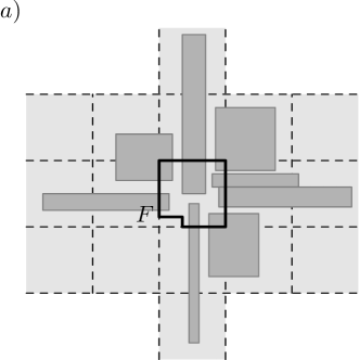
Let be a face which is not a rectangle face, and which is not contained in a single grid cell. We will show that is contained in a single row or column of grid cells. Assume, for contradiction, that is not contained in a single row or column of grid cells. Then there must be a grid cell with vertical and horizontal edges and , respectively, such that and . As , and therefore , Proposition 27 and Proposition 28 give us that is crossed both by horizontal and vertical rectangles from , which gives contradiction. The face must be contained in a single row or column of grid cells.
Assume w.l.o.g. that is contained in a single column of grid cells, but not in a single grid cell (see Figure 7b). Then for each grid cell for which , is contained between the lines and which are parts of edges of vertical rectangles crossing . In particular, no rectangle from can intersect and . If a rectangle from has non-empty intersection with , then it must be contained in the same column of grid cells as , i.e., all rectangles intersecting are contained in a stripe of of width , and have total weight at most .
As the boundary of a rectangle face does not intersect any rectangles from , we instantly get that the boundary of any face intersects rectangles from of total weight at most . ∎
Proof of Lemma 12.
From Lemma 9 each rectangle from can be intersected by at most edges of the graph . That gives us that the total cost of edges in is at most .
From Lemma 10 each face of which is not a rectangle face has non-empty intersection with rectangles from of total weight at most , and so the weight of is at most .
As each rectangle intersecting faces contributes to the weight of each of the faces, the total weight of the faces is . ∎
Proof of Lemma 13.
Let be the set of lines, and the graph constructed for the set of rectangles . From Lemma 8 is planar, and so we can apply Theorem 11 to the embedding given by the lines .
Let be the V-cycle of from Theorem 11 for . We will transform into a cycle which uses only ordinary edges of . We consider the face edges one by one, and we substitute each face edge for a face with a path in connecting and and using only edges which are on the boundary of . We can choose this path in two ways, depending on whether we want to become a part of the interior, or the exterior of . We always merge with the part of lower weight. Notice that might not be a simple cycle, but we can always modify so that each edge appears only times in .
We will show that the cycle gives a balanced -cheap -cut. From Lemma 8 we get that . The cycle uses edges, and so is a -cut.
We will now upper bound the total weight of rectangles from intersected by . From Theorem 11 the ordinary edges of have cost , which from Lemma 12 is , and so they intersect rectangles from of a total weight . The remaining edges of lie on the boundaries of at most faces, and from Lemma 10 the boundary of each face intersects rectangles of weight . The edges of intersect rectangles of total weight , and so is a -cheap cut.
From Theorem 11 the interior and the exterior of have weights at most , and from Lemma 12 we get that . Each rectangle in has weight smaller than , and so the weight of each rectangle face of is smaller than . From Lemma 12 the weight of any other face of is at most , which is also smaller than for . From the construction of the interior and the exterior of have weights at most . The cut is balanced. ∎
Proof of Theorem 14.
From Lemma 13, for any and for any set of pairwise non-overlapping rectangles which does not contain a rectangle of weight at least there exists a balanced -cheap -cut for some constant .
Applying Lemma 4 gives us, that the algorithm GEO-DP has approximation ratio when parametrized by some . Let us fix such that the approximation ratio is at most . Such choice of requires . The running time of GEO-DP is then according to Proposition 2, and so GEO-DP is a QPTAS for the maximum weight independent set of rectangles problem. ∎
Appendix C Complete Construction of
For any two points we denote by the straight line from to . Also, we define .
For each endpoint of a line such that does not hit a perpendicular line in at we will create a path of lines connecting with a line in , and we will add the constructed lines to the set . Ideally, we would like the added lines to intersect no blocks. However, as we want the size of the partition to be small, we will have to allow the lines to cut some blocks.
Before we show the construction of the paths, we need the following lemma. Note that it holds for arbitrary lines , and not only for lines in .
Lemma 29.
Let be a grid cell and . Let be a line which does not intersect any blocks and lines from , which has one endpoint at , and the other endpoint outside of . If hits a perpendicular block at , but it does not hit a perpendicular line from at , then:
-
•
, and
-
•
one end of is in , and the other one is outside of .
Proof.
Assume w.l.o.g. that is vertical, is at the top end of , and crosses the boundary of the grid cell to the right of . Let be the maximal line which contains the bottom edge of and does not intersect any blocks or lines from . As , we get that .
Assume that is at the boundary of . If lies on the bottom or right edge of , is the bottom-most long line crossing the right edge of . If lies on the top edge of , is the top-most long line crossing the right edge of . If lies on the left edge of , is the bottom-most long line crossing the left edge of . In each of the cases we have that , which gives a contradiction.
As , intersects . If does not end in , then cuts . If is the bottom-most sticking-in line for the left edge of then , which gives a contradiction. Otherwise, the bottom-most sticking-in line for the left edge of is below and cuts , so it intersects , and again we get a contradiction, as does not intersect edges from . Block must end in . ∎
We now present the construction of the paths. For each endpoint of a line such that does not hit a perpendicular line in at , we construct a set of lines as follows. Let be a grid cell such that , and let be the block hit by at . Such a block exists, as is maximal, and does not hit a line from at . The line together with , and satisfy the conditions of Lemma 29. We get that , and has one end in . Let be the grid cell with the other end of . Let be a maximal line which contains the edge of containing , and does not intersect any blocks or lines from . Let be the endpoint of such that . We set . We know that , so intersects at least two grid cells. See Figure 8 for a sketch.
We fix a parameter . We have to consider the following cases:


-
1.
There is a line such that (see Figure 8a). Such a situation can happen, as lines from are not necessarily maximal. As does not hit at and cannot be extended beyond , we get that . The construction of the path is finished.
-
2.
Case does not happen, but hits a line from at , (see Figure 8b). The construction of the path is finished.
-
3.
Cases and do not happen. In this case, hits some perpendicular block at (see Figure 8c). We proceed as before, considering the line and its endpoint instead of and . The conditions of Lemma 29 are satisfied, as intersects at least two grid cells. We continue extending the path, until one of the cases or applies, or the number of lines in the path reaches the upper bound .
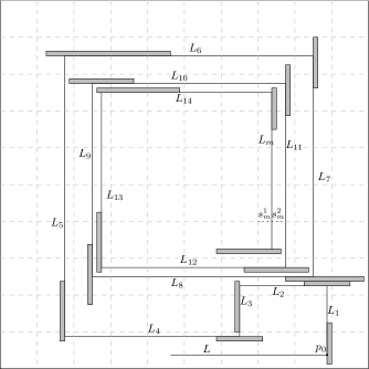
Let be the collection of lines obtained as described above, for some . We have . We modify the set as follows. If the construction of the set ended in case , we add the set of lines to . Let be the line contained in . We extend , so that it has an endpoint in . Notice, that all the lines which were touching after extending are still touching . If the construction of the set ended in case , we add the set of lines to .
Let us now consider the difficult case, i.e., when after steps the path does not hit any line from . We do not want to extend the path any further, as the number of lines in would become too large. We have to find a place to create a "shortcut" which connects some part of the path to a line from , cutting some blocks. We will ensure that the rectangles cut during this operation have small total weight. The cut will go along the boundary of some grid cell. An example can be seen on Figure 9.
Each line intersects least two grid cells. For each let be the grid cell in which ends, i.e, such that . From the construction of the path we know that . Let be the edge of intersected by , and let . Let and be the segments on which connect with the two neighboring lines from , i.e. for we have such that and , and .
We will show that such segments always exist. crosses the edge of , and the maximal line containing which does not intersect any blocks or lines from is long (as at least some part of goes along a long edge of a block). As , lies between two lines from — the leftmost and the rightmost long lines crossing the edge of , and so the segments and are contained in . A segment possibly cuts some blocks. Let be the set of rectangles cut by .
Lemma 30.
Any rectangle belongs to at most four sets , where and .
Proof.
If is not contained in a single row or column of grid lines, it cannot be cut by any segment , and so it does not belong to any set . Assume w.l.o.g. that is vertical and it is inside a single column of grid cells. Let and be the grid cells where the blocks of end.
Let be a grid cell boundary which intersects such that and . Let and be the grid cells for which . crosses and , and so the vertical sticking-in lines in and cross and , and is contained between them. If a line ends in or , its end cannot lie between the sticking-in lines (as there are no perpendicular blocks which could be hit by ), and so for , and .
At the boundary of or the rectangle can be cut by at most two segments and , such that , and . ∎
From Lemma 30 we get that there is a line in and a segment for which . We have two cases:
-
•
connects the line with a line from .
We then continue the path from only until the point , and then extend it by the segment . Formally, we add the lines , the line and the segment into .
-
•
connects the line with a line for .
We then continue the path from until the intersection of with , and then extend it by the segment . Let . Formally, we add the lines , the line and the segment into .
We do this procedure iteratively for all endpoints of a line which are not connected to some other line in , i.e., if , for the so far computed set .
Appendix D Proofs from Section 4
Proof of Lemma 16.
We will start by showing that the set of lines is nicely connected. From the construction of the lines it is clear that no two lines from overlap or intersect properly. We need to show that for any line and any endpoint of there is a line perpendicular to such that .
For each endpoint of a line which does not hit a perpendicular line from we added a perpendicular line touching to the set . The path of lines connecting with a line from is constructed in such a way, that each line added to has both endpoints touching perpendicular lines from . If a line from gets extended, it is extended in such a way that the new endpoint touches a perpendicular line from . The set of lines is nicely connected.
We will now show an upper bound on . From Proposition 15 the set consists of lines. For each endpoint of a line from , except from the four lines in bounding the input square, we added at most lines to the set , which gives .
We will now upper bound the total weight of rectangles from which are cut by a line from parallel to their shorter edge. The only lines from which cut rectangles along their shorter sides, i.e., which cut all blocks corresponding to a given rectangle, are the lines from which correspond to segments . Each segment cuts only the set of rectangles , and we add to only such segments , for which . The number of segments added to is upper bounded by . That gives an upper bound of (as ) on the total weight of rectangles from which are cut by a line from parallel to their shorter edge.
From the construction of the lines it is clear that all lines from cutting rectangles in lie on grid lines, and a line from cannot be contained in the interior of a grid cell. ∎
Proof of Lemma 17.
First we prove some additional lemmas.
Lemma 31.
Let be a line and let be a grid cell such that is a sticking-in line (not necessarily extremal) for an edge of , and does not cross . Let be an endpoint of . Then there exists a line perpendicular to such that , does not end at and is an extremal sticking-in line for an edge of perpendicular to .
Proof.
From Lemma 16 the set of lines is nicely connected, which means that there is a line perpendicular to such that . We will show that satisfies the remaining conditions of the lemma statement. Without loss of generality we assume that is the bottom edge of .
Let be a maximal line containing which does not intersect any blocks or lines from . We will show that is the bottom-most sticking-in line for an edge of . As is a sticking-in line for and does not cross (i.e. does not touch the edge of parallel to ), cannot be extended at . Either hits at , or hits a perpendicular block at . In either case does not end at .
We first show that is a long line (i.e. longer than the grid granularity). If , then is long and so is . If then, from the construction of , goes along a long edge of a block, and is long as it contains a long edge of a block.

is not contained in , i.e., it intersects an edge of perpendicular to (see Figure 10). Let be a line which intersects below . As cannot intersect and extends beyond , we get .
If crosses , then it is the bottom-most line intersecting and maximizing the length of the intersection with . Assume that does not cross . As is a maximal line which does not intersect any blocks or lines from , it ends in by hitting a perpendicular line from or a perpendicular block. This line or block does not intersect the bottom boundary of , as it would yield a long line crossing which reaches further than , which gives a contradiction, as is a sticking-in line for . The line or block hit by crosses the top edge of and does not intersect any lines from . Therefore any line which intersects above satisfies .
We get that is the bottom-most long line maximizing the length of the intersection with , and so it is the bottom-most sticking-in line for . We get that , and so . satisfies all conditions of the lemma statement. ∎
Lemma 32.
Let be a grid cell, and let be an edge of . Let be two lines intersecting , touching at and respectively, such that there is no line which intersects and touches between and . Then there is an edge of and lines touching such that , .
Proof.
First observe that the lemma statement allows that or .
Assume w.l.o.g. that is the bottom edge of , is on the left of , and that . We have to consider three cases. We start with the most interesting case, where both and do not cross . Let and be the endpoints of and , respectively, in . Let and be two lines from perpendicular to and such that and , respectively. From Lemma 16 such lines exist and they are not contained in , i.e., each of them touches an edge of . If touches the right edge of , then also touches the right edge of and we are done (see Figure 11a). If touches the left edge of , then , and we are done (see Figure 11b).


The only remaining possibility is that touches only the left edge of , and only the right edge of (see Figure 11c). As there are no edges in intersecting and touching in between and , is a sticking-in line for the edge of . From Lemma 31 is the bottom-most sticking-in line for the left edge of , and it does not end at . does not touch the right edge of , and applying Lemma 31 to gives us that hits a perpendicular sticking-in line in . does not touch the bottom edge of , as we would have , and is a sticking-in line. touches the top edge of , and is a sticking-in line for this edge. As ends in , applying Lemma 31 to gives, that it hits a perpendicular (i.e. touching the right edge of ) sticking-in line . Either , or is above , so does not hit , or any line to the right of . Applying Lemma 31 to gives that hits a perpendicular sticking-in line, and the only candidate for such a line hit by is . touches and touches the right edge of , and we are done.
In the second case the line touches the top edge of , and does not. Let be the perpendicular line touching at its endpoint . From Lemma 16 such line exists and is not contained in . As is to the left of , touches the right edge of (see Figure 11d). Let be a sticking-in line for the right edge of . Such line exists, as the maximal line containing is a candidate for it. We will show that touches . If crosses , then must touch (and either or goes along an edge of ). If does not cross , from Lemma 31 we get that hits a perpendicular sticking-in line in . As is the rightmost line crossing (all lines to the right of cannot exceed ), it is the rightmost sticking-in line and touches . We set .
In the last case, when both and touch the upper edge of , the claim is immediate (see Figure 11e). ∎
First we will consider the case when has non-empty intersection with some block contained in . Let be an edge of such that . Assume w.l.o.g. that is the bottom edge of (see Figure 12a). Let be lines which intersect and touch at some points and , respectively, such that is to the left of , is to the right of , and no line from which intersects touches in between and . Such lines exist, as no line from intersects inside , the leftmost long line intersecting and touching (which belongs to ) either contains the left edge of or is to the left of it, and the rightmost long line intersecting and touching (which also belongs to ) either contains the right edge of or is to the right of it.
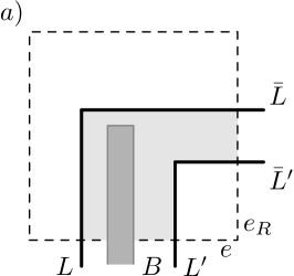
Parts of the lines lie on the boundary of . Denote by and the lines given by applying Lemma 32 to and . If and both intersect the top edge of then the claim follows and in particular is the interior of a rectangle. Otherwise, assume w.l.o.g. that they intersect the right edge of and assume w.l.o.g. that is the bottommost line touching and and is the topmost line touching and . From Lemma 16 the set of lines is nicely connected, and by construction, all lines in with non-empty intersection with for some grid cell touch the boundary of Q. Hence, there can be no line in intersecting between and . Hence, the claim follows.
We already know that the lemma holds for any connected component of for any grid cell such that has non-empty intersection with for some block contained in . Now we will show that if the lemma is satisfied for some connected component of , then it is also satisfied for a connected component of if (see Figure 12b). That will prove the lemma.
Let , and let . Let be lines bounding and touching . From the construction above we know that such lines exist. We want to show that there are two lines intersecting and touching such that and there are no lines intersecting and touching in . Then, by proceeding exactly as in the first case, we prove the lemma.
Assume w.l.o.g. that is a vertical edge and that is above . We show only that there is a line intersecting and touching above (with a similar reasoning one can show that there is a line intersecting and touching below ). Let be the top-most horizontal line in intersecting and touching . We will first show that such line exists and it is not below . If , then either or is above and we are done. Otherwise and, from the construction of , goes along a long edge of a block, and the maximal line containing which does not intersect blocks and lines from is long. As , there must be a line which is above .
If intersects , we set and we are done. Otherwise, observe that and hence it is maximal. We claim that hits a perpendicular line at (and, as the name suggests, it will turn out that crosses the top edge of ). As is maximal, it has to hit a perpendicular block or a perpendicular line from at its endpoint in . If the first case occurs, then the maximal long line going along the left edge of is the leftmost long line intersecting the top edge of , and it belongs to . We get that hits a perpendicular line at its endpoint in . We cannot have , as the maximal long line containing is the leftmost long line intersecting the top edge of , and so it belongs to . We have that .
As we have that . Thus, ends above by hitting a perpendicular line or a perpendicular block . In the first case we are done. In the second case, the topmost long line intersecting and touching contains the upper edge of and crosses above . Hence, we can set and we are done. ∎
Proof of Lemma 18.
Let . Let be a connected component of containing . We get that , and so there exists a component which satisfies the desired properties.
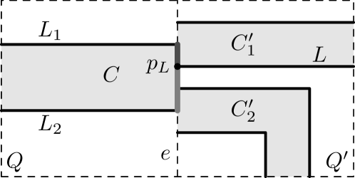
We now show that is unique. Assume otherwise, i.e. that there are two connected components and of which have non-empty intersection with . Let be a line intersecting , such that is between and (see Figure 13). Such line exists, as and are not connected. Let be the lines intersecting , touching and bounding . Then there is no line which intersects and touches between and . As is between and , it holds that is between and . That gives us that cannot intersect , and so has an endpoint . We will now show that one of the segments and is contained in , which gives contradiction, as it requires or . Hence, the component is unique.
We will now show the following lemma.
Lemma 33.
Let and be two neighboring grid cells and let . Let be a maximal segment of contained in , and assume that does not contain any endpoint of . Then is incident with lines (where possibly ) such that intersects and intersects .
Proof.
From the construction of and , the segment consists of one or multiple segments , as any other line from would touch an endpoint of . Let be the first one added to . W.l.o.g. assume that in the construction of the path, the line preceding on the path intersects . Let be the line perpendicular to which is at the other end of . If intersects , we are done. Assume, for contradiction, that intersects and has an endpoint at . We have that does not hit a perpendicular line from at as otherwise such a line would be contained in the leftmost long line crossing the top or the bottom edge of which are by definition in and the segment has by construction non-empty intersection with all lines in . Assume that . From the construction of , in particular from Lemma 29, we get that the successor of on the path must be a segment (as if was not "shortened", it would end in the interior of a grid cell). Then is neighboring to the segment , which has been added to before . As then from the maximality of , we get a contradiction, as was the first segment from added to .
Assume that . Then, as is maximal and it does not hit a perpendicular line from at , hits a perpendicular block at . The long edge of containing is then an extremal long line crossing an edge of perpendicular to , and do it belongs to . We get a contradiction, as does not hit a perpendicular line from at .
We obtain that intersects , which proves the lemma. ∎
As is an endpoint of , touches a perpendicular line from at . Let be a maximal segment of containing and contained in . From Lemma 33 segment contains an endpoint of , or is incident with a line intersecting . In any case, one of the segments , is contained in , i.e. it is contained in . ∎
Proof of Lemma 19.
From Proposition 15 we get that . From Lemma 16 . For any line the number of rectangles intersected, but not cut by is at most . As the length of is at most , the number of rectangles cut by such that is smaller than . The number of circumvented polygons is therefore at most . Circumventing a polygon generates four lines in , and possibly splits some lines from in two. The number of lines in is at most .
The added lines do not intersect rectangles. The only rectangles intersected by a line in are the rectangles cut by a line from parallel to their shorter edge. From Lemma 16 the total weight of such rectangles is upper bounded by . ∎
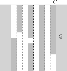
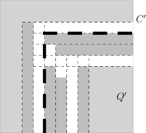
Proof of Lemma 20.
We first prove the lemma for the setting that each rectangle is a block, i.e., for each we have or . Consider a face which is homeomorphic to a line. For each grid cell and for each connected component of we will define a set of lines . Due to Lemma 17 the component is either a rectangle or an L-shape (note that here we can have a "degenerated L-shape" with only four edges). If is a rectangle, we consider any edge of such that , and we define to be the set of all maximal lines perpendicular to , with integer endpoints, which are contained in or in the boundary of (see Figure 14). Observe that if all rectangles are blocks, the lines in do not intersect any rectangles. Now consider the case when is an L-shape and let be the (perpendicular) edges of such that . (Notice that we can have a special case that intersects only one edge of , i.e., the face does not extend beyond . However, then we take as the edge of perpendicular to which contains the boundary edge of perpendicular and non-adjacent to . Intuitively, that is the edge where the face would continue beyond if it was not blocked by a line from .) We define to be the set of all pairs of straight lines with integer endpoints contained in , which do not intersect any blocks, and such that is perpendicular to and to , and there is a point such that has one endpoint at and the other one at , and has one endpoint at and the other one at (see Figure 14).
Next, we define a family of faces contained in the face . Each face will have bounded complexity (i.e., at most boundary lines). We will construct in such a way that and each face in which is not a rectangle of unit height or width can be decomposed into a bounded number of subfaces in without intersecting any block. During the recursion of GEO-DP, when parametrized with large enough , the algorithm will consider exactly this decomposition. Thus, GEO-DP optimally solves the subproblem induced by the face .
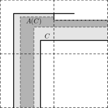
Now we define the family . For any grid cell and for any connected component of we select two elements from the set of lines , allowing to select the same element twice, but not allowing the two chosen elements to intersect properly. Let denote the subarea of which is strictly between the two selected elements from (i.e., the chosen elements from do not belong to ), see Figure 15. We require the selected elements for the different components to be consistent, meaning that for any two connected components of within some grid cells such that we have (i.e., the subareas chosen for different grid cells match at the boundaries of the grid cells), and is connected. For any choice of consistent elements for all connected components we add to . Due to the definition of , every face in which is not a rectangle of unit height or width can be decomposed in two disjoint elements of . Every face in which is a rectangle of unit height or width contains at most blocks, and GEO-DP finds an optimal solution for it.
The decomposition can be seen as follows. Let . Take a component of within a grid cell which is a dead-end, i.e, there is only one edge of such that . Draw a line splitting into two components without intersecting any block, such that one end of the line touches the boundary of (if is an L-shape we might need two lines for that). We take the loose end of and extend it until we touch the boundary of or we hit a perpendicular block. In case we touch the boundary of , we are done. If hits a block at some point , we continue similarly as in case of loose ends of the lines in . We draw a new line starting at and following the edge of so that we cross a grid cell boundary. We continue iteratively until we draw a line whose end touches the boundary of . Then the lines define a path splitting into two subpaths. See Figure 6.
It remains to upper bound the complexity of the faces in , i.e., bound the number of their boundary edges. By definition, the latter quantity is in the order of the number of connected components of for all grid cells . The reason is that for each face the boundary of a connected component of (for any grid cell ) has only a constant number edges. As the number of lines in is upper bounded by (see Lemma 19) and there are grid cells, the number of such components is upper bounded by .
We conclude that if all rectangles are blocks, GEO-DP finds an optimal solution for if . For the case of arbitrary rectangles we observe that the boundary of each face in intersects rectangles from contained in only parallel to their longer edges. Hence, for any face there are only rectangles which are contained in and intersected by the boundary edges of . Hence, whenever in the above argumentation we decompose a face into two disjoint elements , we can instead argue that the face is decomposed into the faces and and the at most rectangles . Also, again each face has a boundary with at most edges. Note that in this case can consist of multiple (at most ) connected components and GEO-DP recurses on each of them separately. Hence, in the case of arbitrary rectangles, GEO-DP parametrized with finds an optimal solution for . ∎
Proof of Lemma 21.
Like in the proof of Lemma 20 above, let us first assume that all rectangles are blocks. Consider a face which is homeomorphic to a cycle. We now describe a procedure to draw a path consisting of a set of lines , which will either add further structure to so that it becomes a path-face or will subdivide into a cycle-face and a path-face. The endpoints of the lines will have integer coordinates, and their number can be arbitrarily large (in particular, larger than etc.). The lines will not intersect any blocks contained in .
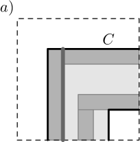
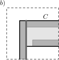
Consider an arbitrary connected component of for some grid cell , such that is an L-shape. Such a component exists since otherwise would not be a cycle. It is always possible to draw a line within which does not intersect any blocks and which subdivides into a rectangle and an L-shape or into two rectangles (see Figure 16). In the second case the line transforms into a path-face and we are done. Now consider the first case. We define as a maximal line containing which does not intersect any block and which does not cross the boundary of or overlap an edge from the boundary of . If both endpoints of touch the boundary of , we are done. Otherwise, we continue very similarly as in the construction of the lines . Let be an endpoint of which hits a perpendicular block . Observe that this must happen within a connected component of where is an L-shape. As is large, one of its endpoints must lie outside of . Denote by the maximal line within containing and going along the edge of which does not intersect any blocks. Denote by the endpoint of which is outside of . We define and continue iteratively. Observe that in contrast to the definition of the lines , we do not stop after some fixed number of iterations, but continue until the added line either touches the boundary of , or hits some line with . Let . If the path touches both boundaries of the cycle-face , it transforms into a path-face. Otherwise (i.e., if the path touches the same boundary twice or ends by hitting itself), the path subdivides into a path-face and a cycle-face .
As in the proof of Lemma 20, we can formulate as the union of sets , where for each component we select two elements from the set . For each component we do this as follows. If is not intersected by the path , we choose the two elements of going along the boundaries of . Otherwise, if does not end in , we select the element in which is given by the last line(s) in crossing and one element which describes the boundary of not touched by . If ends in , we also select the boundary of not touched by , and additionally an element in which consists of and a segment of of where denotes the penultimate line in crossing . With a similar reasoning as in the proof of Lemma 20, we can then upper bound the complexity of the boundaries of by . See Figure 17 for an example of the described operation.
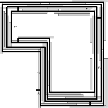
Now let us focus on . In case the boundary of is more complex than our upper bound of edges allows, we split into a set of consecutive paths , each of them having a boundary whose complexity is at most . We perform these necessary cuts along grid lines. Each connected component of is a rectangle or an L-shape (where we treat a rectangular component within a cell like an L-shape if for two perpendicular edges of ). Let be the set of all consecutive connected components of within single grid cells such that is an L-shape. For each -th component , starting with a random offset, we cut inside , along a grid cell boundary (intuitively, we cut after every bends). There is an offset for which the total weight of intersected blocks is at most a -fraction of the total weight of the blocks in . Each resulting path can be expressed as the union of a set of at most components, where each component is a rectangle or an L-shape within some component of , and therefore the complexity of is at most .
One can show, in the same way as when upper bounding the complexity of the boundary of , that for any the total boundary of each set has at most edges. Hence, GEO-DP parametrized with tries to partition step by step, in the -th step splitting off the path from the remaining area of . Finally, it partitions into path-faces and a cycle-face . Knowing from the proof of Lemma 20 that GEO-DP solves the subproblem for each path optimally if is sufficiently large compared to the length of the path, we conclude that GEO-DP parametrized with computes a solution for with weight at least . By continuing with the same arguments for , in case , we get that GEO-DP computes a solution for whose weight is at least .
With similar adjustments as in the proof of Lemma 20 we show that the same is true in the setting of arbitrary rectangles at the cost of an increase in complexity by a factor of .∎
Proof of Theorem 22.
Fix . For each set of rectangles and for each polygon in the original input instance there is a corresponding polygon, containing the same subset of rectangles, in the instance obtained after the preprocessing performed by GEO-DP (which ensures that all corners of rectangles have coordinates within , where ). Hence, it suffices to show that GEO-DP, when executing without the preprocessing routine, achieves the claimed approximation ratio on the original input instance.
Let be an optimal solution for a given instance of the problem, and let be the set of lines constructed for . From Lemma 19 we have , and so partitions the original input square into at most faces, and GEO-DP will consider such a partition of the input square. From Lemma 19, the total weight of intersected rectangles from the optimal solution in this partition is upper bounded by . When recursing on each resulting face, due to Lemmas 20 and 21 GEO-DP obtains a -approximative solution for each subproblem. Thus, in total we obtain an approximation ratio of .
When GEO-DP performs the preprocessing first, in the modified input instance it will consider the same recursive partitioning of the input square, obtaining the same approximation ratio. From Proposition 2, the running time of GEO-DP parametrized with is upper bounded by , and so it yields a PTAS for -large rectangles for any constant . ∎
Proof of Corollary 23.
Suppose that we are given an input instance for which there is a value such that for any rectangle we have , and all input coordinates are within for some integer . We define a grid with offset whose grid cells have height and width , i.e., we define a cell for each .
Since for each rectangle , when choosing a random offset , in expectation the intersected rectangles from an optimal solution have a total weight of at most . We take this random offset and consider the resulting subproblems in each grid cell which contains at least one input rectangle (there can be at most such grid cells), i.e., each subproblem consists of the original instance restricted to the rectangles contained in the respective grid cell. Since each grid cell has height and width and for each rectangle , we conclude that each grid cell constitutes a subinstance in which all rectangles are -large. During the recursion process, GEO-DP guesses exactly this subdivision (not all at once but e.g., in a quad-tree fashion). Using Theorem 4 we know that GEO-DP computes a -approximation for each of them, given that . Altogether, we obtain a -approximation algorithm for the overall problem. ∎