MYE: Missing Year Estimation in Academic Social Networks

Abstract

In bibliometrics studies, a common challenge is how to deal with incorrect or incomplete data. However, given a large volume of data, there often exists certain relationships between the data items that can allow us to recover missing data items and correct erroneous data. In this paper, we study a particular problem of this sort - estimating the missing year information associated with publications (and hence authors’ years of active publication). We first propose a simple algorithm that only makes use of the “direct” information, such as paper citation/reference relationships or paper-author relationships. The result of this simple algorithm is used as a benchmark for comparison. Our goal is to develop algorithms that increase both the coverage (the percentage of missing year papers recovered) and accuracy (mean absolute error of the estimated year to the real year). We propose some advanced algorithms that extend inference by information propagation. For each algorithm, we propose three versions according to the given academic social network type: a) Homogeneous (only contains paper citation links), b) Bipartite (only contains paper-author relations), and, c) Heterogeneous (both paper citation and paper-author relations). We carry out experiments on the three public data sets (MSR Libra, DBLP and APS), and evaluated them by applying the K-fold cross validation method. We show that the advanced algorithms can improve both coverage and accuracy.

1 Introduction

Academic publication analysis has always been of interest to the research community. Earlier focus includes citation analysis and journal impact factor analysis, to help evaluate research impact. In recent years, there has been an increasing interest in the social aspects of this research, for example, there exist studies of patterns of collaborations, automatically inferring advisor-advisee relationships, and finding or predicting leaders and rising stars in research areas. A common challenge to such research is how to deal with the lack of data, or when data is available, its incorrectness and incompleteness. However, since the data volume is large, and there exists all kinds of relationships between data items, it is often possible to recover certain missing (or correct erroneous) data items from the data we have. In this paper, we study a particular problem of this sort - estimating the missing year information associated with publications (and hence the authors’ years of active publication).

Recently, data cleaning on academic social networks has received much attention. In KDD Cup 2013, the two challenges are the Author-Paper Identification Challenge and the Author Disambiguation Challenge. For both challenges, the publishing year information of each paper is important background knowledge for the design of algorithms. However, the given data set KDDCup (2013) has a high Missing Year Ratio, $\frac{155784}{2257249}\approx 6.90\%$ (there are in total 2,257,249 papers, and out of which, 155,784 are missing year papers). This is important motivation for developing algorithms to recover the missing year attribute of publications, we called this the Missing Year Estimation (MYE) problem.

The occurrence of the missing data in the bibliographic data can be caused by a variety of reasons. We believe one reason is that the cited papers are also included in the dataset, even if the original source is unavailable. References are sometimes incomplete, leading to missing and erroneous data. It is also possible that some papers are recovered from scanned sources which makes it hard to extract all attributes.

We first propose a simple algorithm that only makes use of the “direct” information, such as paper citation/reference relationships or paper-author relationships. The result of this simple algorithm is used as a benchmark for comparison. Our goal is to develop sophisticated algorithms that increase both the coverage (measured by the percentage of missing year papers recovered) and accuracy (mean absolute error, or MAE, of the estimated year to the real year). The more advanced algorithms we propose and study involve information propagation rules so that information which is multiple hops away can also be utilized. For each algorithm, we propose three versions according to the given academic social network type: a) Homogenous (only contains paper citation links), b) Bipartite (only contains paper-author relations), and, c) Heterogeneous (both paper citation and paper-author relations). We carry out experiments on the three public data sets (MSR Libra, DBLP and APS), by applying the K-fold cross validation method.

Our contributions are: we formulate the problem and introduce a basic (benchmark) algorithm that can already recover most of the missing years if both citation and author information are available. We then systematically developed improved algorithms based on methods in machine learning. These advanced algorithms further improve both coverage and accuracy (around $20\%$ in the paper citation network, $8\%$ in paper author bipartite network and heterogeneous network), over the benchmark algorithm. In addition, the coverage achieved by the advanced algorithms well matches the results derived by the analytical model.

The remaining of the paper is organized as follows; we first introduce the estimation methodology in section 2, then we describe the data sets used and the experiment results in section 3. In section 4, we discuss the related works and lastly conclude our work in section 5.

2 Methodology

In this section, we first introduce the notations and the three types of the academic social networks we are dealing with. For each network type, we propose three corresponding missing year estimation (MYE) algorithms, with different complexity levels.

2.1 Notations and three types of the network

In a general academic social network, there are many types of nodes and edges. For example, node types can be papers, authors and publishing venues, etc; and edges can be citations (linking papers to the papers they cite; authorships (connecting authors to the papers they have written), and so on.

In the MYE problem, we are mainly interested in two node types: papers and authors; and two edge types: paper citations and paper authorships, which induce three academic social networks:

1. Paper citation network, denoted by a directed graph $G_{P}=(V_{P},E_{P})$, where $V_{P}$ is the set of papers and $E_{P}$ is the set of citation links. Since citation links have directions, each citation link can be represented by an ordered paper pair, i.e., $\forall e=(t,f)\in E_{P}$, where $t,f\in V_{P}$, meaning this citation link is pointing to paper $t$ and originated from paper $f$.

2. Paper authorship network, denoted by $G_{AP}=(V_{A}\cup V_{P},E_{AP})$, where $V_{A}$ is the set of authors, $V_{P}$ is the set of papers and edges in the set $E_{AP}$ connecting authors to their produced papers (authorship). Hence $G_{AP}$ is a bipartite graph and we have $\forall e=(a,p)\in E_{AP}$, where $a\in V_{A}$ and $p\in V_{P}$.

3. Heterogenous network, consisting of both paper citation network and paper authorship network, denoted by $G=(V_{A}\cup V_{P},E_{P}\cup E_{AP})$.

Papers are further categorized into two exclusive sets: with known year information $V_{P}^{K}$ and unknown (missing) year information $V_{P}^{U}$. Hence we have $V_{P}=V_{P}^{K}\cup V_{P}^{U}$ and $V_{P}^{K}\cap V_{P}^{U}=\emptyset$. The remaining notations are listed in Table 1:

Table 1: List of Notations

$Y(p),\;\forall\;p\in V_{P}$	the real publishing year of paper $p$, note:
	$\forall\;p^{U}\in V_{P}^{U},Y(p^{U})$ is only used for validation purpose.
$T(p),\;\forall\;p\in V_{P}$	the set of papers that cite paper $p$,
	i.e., $T(p)=\{f|\forall f\in V_{P},s.t.,(p,f)\in E_{P}\}$.
$F(p),\;\forall\;p\in V_{P}$	the set of papers that are cited by paper $p$,
	i.e., $F(p)=\{t|\forall t\in V_{P},s.t.,(t,p)\in E_{P}\}$.
$\hat{Y}(p^{U}),\;\forall\;p^{U}\in V_{P}^{U}$	the estimation result for the missing year paper $p^{U}$.
$P(a),\;\forall\;a\in V_{A}$	the paper set that are written by author $a$.
$A(p),\;\forall\;p\in V_{P}$	the author set that have written paper $p$.
$w(p,q),\;\forall p,q\;\in V_{P}$	the Consistent-Coauthor-Count between two papers,
	$w(p,q)=w(q,p)=|A(p)\cap A(q)|$
$\Omega(p),\;\forall\;p\in V_{P}$	the Consistent-Coauthor-Pair set of a paper $p\in V_{P}$,
	$\Omega(p)=\{q|q\in V_{P}\;\textrm{and}\;w(p,q)>1\}$
$AW\_Min(a),\;AW\_Max(a),$	the lower and upper bounds of the active publishing
$\forall\;a\in V_{A}$	time window of author $a$.
$\hat{Y}_{CMin}(p^{U}),\hat{Y}_{CMax}(p^{U}),$	the lower and upper bounds of the year estimation
$\forall\;p^{U}\in V_{P}^{U}$	window, derived in the paper citation network $G_{P}$.
$\hat{Y}_{AMin}(p^{U}),\;\hat{Y}_{AMax}(p^{U})$,	the lower and upper bounds of the year estimation
$\forall\;p^{U}\in V_{P}^{U}$	window, derived in the paper authorship network $G_{AP}$
$\hat{Y}_{GMin}(p^{U}),\;\hat{Y}_{GMax}(p^{U})$,	the lower and upper bounds of the year estimation
$\forall\;p^{U}\in V_{P}^{U}$	window, derived in the heterogenous network $G$

2.2 MYE for citation network $G_{P}$

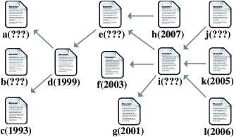
We first look at a simple example of the missing year estimation problem in the paper citation network, shown in Fig. 1. In this example, there are 12 papers ($a-l$) and 10 citation edges. 5 papers ($a,b,e,i,j$) have no year information (i.e. $\in V_{P}^{U}$) and the other 7 papers ($c,d,f,g,h,k,l$) have publishing years (i.e. $\in V_{P}^{K}$). Later on, we will use this example to demonstrate the three MYE algorithms designed for the citation network $G_{P}$.

Figure 1: A simple example of a citation network with 12 papers ($a-l$), where papers ($a,b,e,i,j$) are $\in V_{P}^{U}$ and the remaining ($c,d,f,g,h,k,l$) are $\in V_{P}^{K}$ .

The main idea of estimating the missing years in the citation network $G_{P}$ is to make use of paper citing activities, stated as Assumption 1, together with the available information: a) the year information of those known papers; b) the citation relationships (edges of the $G_{P}$).

Assumption 1

Normally, a paper can only cite those papers published before it, i.e., Eq. (1) is satisfied:

$$Y(t)\leq Y(f),\;\;\forall\;\;e=(t,f)\in E_{P},\;\;t,f\in V_{P}.$$ (1)

Assumption 1 provides the way to determine either a possible upper bound of the target paper’s missing year when it is cited by a known year paper (i.e., $t\in V_{P}^{U}$ and $f\in V_{P}^{K}$); or a possible lower bound of the target paper’s missing year when it cites a known year paper (i.e., $t\in V_{P}^{K}$ and $f\in V_{P}^{U}$). For example, using Fig. 1, we can look at paper $a$ (missing year) and $d$ (published in 1999) with a citation link from $d$ to $a$, we take 1999 as one possible upper bound of $a$’s publishing year, i.e., $Y(a)\leq 1999$. Similarly, when we look at paper $d$ and $e$, we get a lower bound of the real publishing year of $e$, i.e., $1999\leq Y(e)$.

Following this logic, the missing year estimation task can be separated into two steps: (1) deriving the possible year estimation window (two bounds); (2) calculating the missing year value based on the derived window.

For each step, we propose two methods with different complexity, the simple (“Sim”) version and the advanced (“Adv”) version. In the next three subsections, we will introduce the three algorithms designed for MYE in paper citation network $G_{P}$. The three algorithms are different combinations of the two methods in each step, listed in Table 2.

Table 2: Combination of the two proposed methods in each step, for the three algorithms for MYE in $G_{P}$.

Algorithm	Window derivation method	Year value calculation method
$G_{P}$-SS	Simple	Simple
$G_{P}$-AS	Advanced	Simple
$G_{P}$-AA	Advanced	Advanced

2.2.1 Algorithm for MYE in $G_{P}$: $G_{P}$-SS

We will first introduce the simple method for each of the two steps, then we will show how $G_{P}$-SS works by demonstrating the results on the example shown in Fig. 1.

Simple Window Derivation Method: The simple version of the window (bounds) derivation method only involves “one round” (or in a “direct” manner), which means: (1) spatially, we only consider those papers that are one-hop to the target missing year paper; (2) temporally, we only consider immediate (given) information.

Putting together (1) and (2), mathematically, we are deriving the bounds of the missing year paper $p^{U}\in V_{P}^{U}$ through the subset of the papers: $F(p^{U})\cap V_{P}^{K}$ (for the lower bound) and $T(p^{U})\cap V_{P}^{K}$ (for the upper bound) as long as they are not empty. For example, if we look at paper $i$ in Fig. 1, then only $f$ and $g$ (one-hop away from $i$ and with year information) are used for deriving the lower bound, while only $k$ and $l$ for the upper bound. Intuitively, when there are multiple bounds, we will take the tightest one by applying Eq. (2) and (3):

$$\hat{Y}_{CMin}(p^{U}) = \max_{f\;\in\;F(p^{U})\cap V_{P}^{K}}Y(f),\;\textrm{if}\;F(p^{U})\cap V_{P}^{K}\neq\emptyset;$$ (2)

$$= \;\;-\;\infty,\quad\textrm{otherwise};$$

$$\hat{Y}_{CMax}(p^{U}) = \min_{t\;\in\;T(p^{U})\cap V_{P}^{K}}Y(t),\;\textrm{if}\;T(p^{U})\cap V_{P}^{K}\neq\emptyset;$$ (3)

$$= \;\;+\;\infty,\quad\textrm{otherwise},$$

where $\hat{Y}_{CMin}(p^{U})$ denotes the largest possible lower bound of paper $p^{U}$ and $\hat{Y}_{CMax}(p^{U})$ denotes the smallest possible upper bound. Here the $-\infty$ and $+\infty$ have no practical meaning but are used just to represent the non-existent bounds. In the real implementation, they can be assigned to some pre-defined constant variables such as “Default_Win_Min” and “Default_Win_Max”.

Together with the conditions of non-existent bounds, we thus have four types of possible year estimation windows:

Type-1: $$[\hat{Y}_{CMin}(p^{U}),\hat{Y}_{CMax}(p^{U})];$$

Type-2: $$[\;\;\hat{Y}_{CMin}(p^{U}),\quad+\;\infty\quad);$$

Type-3: $$(\quad-\;\infty,\quad\hat{Y}_{CMax}(p^{U})\;\;];$$

Type-4: $$(\quad-\;\infty\quad,\quad+\;\infty\quad).$$

The Type-4 window contains no information for estimation, hence we define Uncovered Paper to be those missing year papers with a Type-4 estimation window. On the other hand, it is possible to make a proper estimation on the year value for the missing year papers with Type-1, Type-2 or Type-3 estimation window.

Simple Year Value Calculation Method: Based on the derived possible year estimation window for each missing year paper $p^{U}$, the next step is to make a guess on its real publishing year. The simple calculation method works in a straightforward way, Eqs. (4)-(7):

Type-1: $$\hat{Y}(p^{U})=\frac{\hat{Y}_{CMin}(p^{U})+\hat{Y}_{CMax}(p^{U})}{2},$$ (4)

Type-2: $$\hat{Y}(p^{U})=\hat{Y}_{CMin}(p^{U}),$$ (5)

Type-3: $$\hat{Y}(p^{U})=\hat{Y}_{CMax}(p^{U}),$$ (6)

Type-4: $$\emph{Uncovered}.$$ (7)

In summary, if both bounds exist (Type-1), we take the average of the two bounds, Eq. (4) (assuming that $Y(p^{U})$ follows any symmetric discrete distribution centered at the middle point of the possible estimation window). If only one bound exists (Type-2 or Type-3), we take the bound value as the calculation result. Otherwise (Type-4), instead of making any random guess, we label it as (Uncovered), which means, the year of such paper cannot be estimated properly. Later on, in the performance evaluation section, we shall consider the uncovered ratio ($=\frac{\textrm{Total \# Uncovered}}{|V_{P}^{U}|}$) of all the proposed algorithms as one of the performance metrics

Considering the example in Fig. 1, we list both the intermediate and final estimation results conducted by apply $G_{P}$-SS in Table 3.

$p^{U}$ in Fig.1	$a$	$b$	$e$	$i$	$j$
$F(p^{U})$	$\emptyset$	$\emptyset$	$d$	$e,f,g$	$i$
$F(p^{U})\cap V_{P}^{K}$	$\emptyset$	$\emptyset$	$d$	$f,g$	$\emptyset$
$T(p^{U})$	$d$	$\emptyset$	$h,i$	$j,k,l$	$\emptyset$
$T(p^{U})\cap V_{P}^{K}$	$d$	$\emptyset$	$h$	$k,l$	$\emptyset$
$\hat{Y}_{CMin}(p^{U})$	$-\;\infty$	$-\;\infty$	1999	2003	$-\;\infty$
$\hat{Y}_{CMax}(p^{U})$	1999	$+\;\infty$	2007	2005	$+\;\infty$
$\hat{Y}(p^{U})$	1999	Uncovered	2003	2004	Uncovered

Table 3: The intermediate and estimation results obtained through $G_{P}$-SS algorithm running on the example of Fig. 1

In Table 3, the first row lists all the 5 papers belonging to $V_{P}^{U}$. The second and third rows list the paper set cited by each of the 5 papers, where the third row only contains papers with year information, e.g. for paper $i$, it cites three papers $F(i)=\{e,f,g\}$ and only two of them have year information, $F(i)\cap V_{P}^{K}=\{f,g\}$. The fourth and fifth rows list the papers that cite each of the 5 papers, where the fifth row only contains papers belonging to $V_{P}^{K}$. The next two rows are the two bounds of the possible estimation window by applying Eqs. (2) and (3), e.g., $\hat{Y}_{CMin}(i)=\max\{Y(f),Y(g)\}=\max\{2003,2001\}=2003$. The last row shows the results derived by the simple year calculation scheme, Eqs. (4)-(7).

The $G_{P}$-SS is simple, quick and easy for both implementation and understanding, but its limitation is also obvious. It has not fully utilized the available information, which results in a high uncovered ratio ($=2/5$ shown in Table 3) and looser bounds. Considering this question, can the information (derived bounds or estimated results after running $G_{P}$-SS) of paper $i$ be useful for its missing year neighbour papers $j$ and $e$? The answer is yes and the next algorithm is designed to deal with this.

2.2.2 Algorithm for MYE in $G_{P}$: $G_{P}$-AS

Comparing to $G_{P}$-SS, $G_{P}$-AS applies the same simple version of year value calculation method, Eqs. (4)-(7), but an advanced method for window derivation with information propagations.

A quick way of extending $G_{P}$-SS is to simply repeat running it. In this way, the estimated result for a missing year paper (e.g. $i$ in Fig. 1) in the previous rounds can be used to derive bounds for its neighbour missing year papers (e.g. $j$ and $e$ in Fig. 1) in the subsequent rounds. However, since the estimated year result for $i$ can be inaccurate, this kind of repeating will definitely propagate and even amplify the inaccuracy.

Advanced Window Derivation Method: Generally in $G_{P}$, for each citation edge linking two papers, there can be three possible conditions: (a) both papers have year information ($\in V_{P}^{K}$); or (b) both papers are missing year ($\in V_{P}^{U}$); or (c) one has year information while the other has not. The limitation of simple window derivation method is that it will only work under condition (c). By rephrasing Eq. (1) as Eq. (8), the advanced window derivation method relaxes this limitation without inducing any inaccuracy in the propagation.

$$\hat{Y}_{CMin}(t)\;\leq\;Y(t)\;\leq\;Y(f)\;\leq\;\hat{Y}_{CMax}(f).$$ (8)

The rationale behind Eq. (8) is to extend the bound transmission rule between two missing year papers: (a) if $\hat{Y}_{CMin}(t)$ exists, it is also a lower bound of $f$; (b) if $\hat{Y}_{CMax}(f)$ exists, it is also an upper bound of $t$. The pseudo code of the advanced window derivation method is included below.

Algorithm 1 The pseudo code of advanced window derivation method

1:  repeat

2:     UpCnt $\leftarrow 0$;

3:     for all $e=(t,f)\in E_{P},t,f\;\in V_{P}$ do

4:        f_CMin_Before$\leftarrow\hat{Y}_{CMin}(f)$;

5:        t_CMax_Before$\leftarrow\hat{Y}_{CMax}(t)$;

6:        if $t,f\in V_{P}^{U}$ then

7:           $\hat{Y}_{CMin}(f)\leftarrow\max\{\hat{Y}_{CMin}(f),\hat{Y}_{CMin}(t)\}$;

8:           $\hat{Y}_{CMax}(t)\leftarrow\min\{\hat{Y}_{CMax}(t),\hat{Y}_{CMax}(f)\}$;

9:        else if $t\in V_{P}^{K}$, $f\in V_{P}^{U}$ then

10:           $\hat{Y}_{CMin}(f)\leftarrow\max\{\hat{Y}_{CMin}(f),Y(t)\}$;

11:        else if $t\in V_{P}^{U}$, $f\in V_{P}^{K}$ then

12:           $\hat{Y}_{CMax}(t)\leftarrow\min\{\hat{Y}_{CMax}(t),Y(f)\}$;

13:        end if

14:        /* Check update counts. */;

15:        if $\hat{Y}_{CMin}(f)\neq\;\;$f_CMin_Before then

16:           UpCnt $\leftarrow$ UpCnt $+1$;

17:        end if

18:        if $\hat{Y}_{CMax}(t)\neq\;\;$t_CMax_Before then

19:           UpCnt $\leftarrow$ UpCnt $+1$;

20:        end if

21:     end for

22:  until UpCnt$\;=\;0$; /* When no update happens, loop ends. */

In Algorithm 1, we first initialize a local variable “UpCnt” which records the total number of bound updates in each loop (Line 2). Lines 3-21 are steps in a loop of processing each citation link of $G_{P}$, where Lines 9-13 are the same as the simple window derivation method, Eq. (2) and Eq. (3), while Lines 6-8 are the essential part that differs from the simple version (also the implementation of the two bound transmission rules of Eq. (8)).

In Table 4, we list both the intermediate and estimation results of applying $G_{P}$-AS on the example of Fig. 1.

$p^{U}$ in Fig.1	Round 1	Round 2	Round 3	$\hat{Y}(p^{U})$
$a$	$(-\infty,1999)$	$(-\infty,1999)$	$(-\infty,1999)$	1999
$b$	$(-\infty,+\infty)$	$(-\infty,+\infty)$	$(-\infty,+\infty)$	NotCovered
$e$	$(1999,2007)$	$(1999,2005)$	$(1999,2005)$	2002
$i$	$(2003,2005)$	$(2003,2005)$	$(2003,2005)$	2004
$j$	$(-\infty,+\infty)$	$(2003,+\infty)$	$(2003,+\infty)$	2003
	UpCnt = 5	UpCnt =2	UpCnt =0

Table 4: The intermediate and estimation results of applying $G_{P}$-AS on the example shown in Fig. 1

From Table 4, we can see that the advanced window estimation takes two rounds (no updates happen in round 3) and the last column is the year estimation results by applying the simple year value calculation method based on the derived bounds. Comparing to Table 3, the improvement is obvious even for this simple example: (1) paper $j$ is no longer labeled as (Uncovered, hence, the uncovered ratio decreases to 1/5; (2) paper $e$ gets a tighter possible estimation window.

So far, we are doing our best to deal with the possible window derivation problem (apparently, paper $b$ in Fig. 1 has no chance of getting a good estimate, and we will discuss the relationship between the uncovered ratio and the structure of the given citation graph $G_{P}$ mathematically in Section 3). In the next algorithm, we investigate how the year value calculation method can be further improved.

2.2.3 Algorithm for MYE in $G_{P}$: $G_{P}$-AA

Given the derived estimation window $[\hat{Y}_{CMin}(p^{U}),\hat{Y}_{CMax}(p^{U})]$ for a missing year paper $p^{U}$, recall Eqs. (4)-(7)(how simple year value calculation method works): (1) if both bounds exist (Type-1), the calculation result is the mean of the two bounds; or (2) if only one bound exists (Type-2 or Type-3), the calculation result equals to the value of the existing bound; or (3) if neither bound exists, then the paper is labeled as Uncovered, representing no proper estimation result.

The year estimation results for cases (1) and (2) affect the accuracy metrics, such as Mean Absolute Error (MAE), while case (3) only affects the uncovered ratio, irrelevant to other metrics. For case (1), it is rational to take the average of the two bounds, since the citing-to activity and cited-by activity can be considered symmetric. However for case (2), more investigation is needed. The physical interpretation of case (2) is based on the assumption that the missing year paper has the same publishing time as the earliest paper that cites it (the upper bound exists), or the latest paper cited by it (the lower bound exists). In reality, this seldom happens. The best guess for a (Type-2 or Type-3) window case may be correlated to the bound value, not just a fixed distance to the bound (e.g. the simple calculation method takes a fixed zero distance). Therefore, the solution for this problem is to find a proper function $\hat{y}(p^{U})=d(WinType(p^{U}),BoundVal(p^{U}))$ to calculate $\hat{y}(p^{U})$ for each missing year paper $p^{U}$, based on its derived estimation window type, denoted by $WinType(p^{U})$ (which takes value of either Type-2 or Type-3), and the value of bound, denoted by $BoundVal(p^{U})$.

To achieve this, we need a separate data set, denoted by $\mathcal{T}$, containing a series of 3-tuple data $t=\{y_{t},WinType_{t},BoundVal_{t}\}\in\mathcal{T}$ for training purpose. Each 3-tuple data corresponds to a missing year paper $t$ in this training set, where $y_{t}$ is the validated real publishing year, $WinType_{t}$ is the derived estimation window type and $BoundVal_{t}$ is the bound value. If we denote $\mathcal{T}_{p^{U}}$ as the subset of $\mathcal{T}$ with respect to $p^{U}$ and $\mathcal{T}_{p^{U}}=\{t|t\in{\mathcal{T}},WinType_{t}=WinType(p^{U}),BoundVal_{t}=BoundVal(p^{U})\}$, then we get the following form for $d(\cdot)$ corresponding with $\mathcal{T}$:

$$\hat{y}(p^{U})=d_{\mathcal{T}}\big{(}WinType(p^{U}),BoundVal(p^{U})\big{)}=\frac{\sum_{t\in\mathcal{T}_{p^{U}}}y_{t}}{|\mathcal{T}_{p^{U}}|},$$ (9)

where $|\mathcal{T}_{p^{U}}|$ is the element count of the set $\mathcal{T}_{p^{U}}$.

The idea of Eq. (9) is to take the expectation of the real publishing years of those papers having the same window type and bound value as $P^{U}$ in the training set $\mathcal{T}$. However it is not trivial to find a proper training set satisfying: (1) a citation graph with similar property and structure to the given $G_{P}$; (2) the $BoundVal$ of this training set covers a wider range than that of $BoundVal(p^{U}),\forall p^{U}\in V_{P}^{U}$.

Advanced Year Value Calculation Method: We first propose a way to find a suitable training set $\mathcal{T}$ which can satisfy both (1) and (2) mentioned above. After that, the estimation results can be calculated through Eq. (9).

One of the most suitable training sets is just inside the given citation network $G_{P}$. In fact, each paper with known year ($\forall p^{K}\in V_{P}^{K}$) can also be used to derive a possible estimation window (by pretending itself to be a missing year paper). Consider the example in Fig. 1, for paper $d(1999)$, the simple window derivation method generates $[1993,+\infty)$. Since this is independent of deriving windows for missing year papers, these two procedures can be merged together to save the running time. The modified advanced window derivation method for $G_{P}$-AA is shown in Algorithm 2.

Algorithm 2 The modified advanced window derivation method for $G_{P}$-AA

1:  repeat

2:     UpCnt $\leftarrow 0$;

3:     for all $e=(t,f)\in E_{P},t,f\;\in V_{P}$ do

4:        f_CMin_Before$\leftarrow\hat{Y}_{CMin}(f)$;

5:        t_CMax_Before$\leftarrow\hat{Y}_{CMax}(t)$;

6:        if $t,f\in V_{P}^{U}$ then

7:           $\hat{Y}_{CMin}(f)\leftarrow\max\{\hat{Y}_{CMin}(f),\hat{Y}_{CMin}(t)\}$;

8:           $\hat{Y}_{CMax}(t)\leftarrow\min\{\hat{Y}_{CMax}(t),\hat{Y}_{CMax}(f)\}$;

9:        else if $t\in V_{P}^{K}$, $f\in V_{P}^{U}$ then

10:           $\hat{Y}_{CMin}(f)\leftarrow\max\{\hat{Y}_{CMin}(f),Y(t)\}$;

11:           $\hat{Y}_{CMax}(t)\leftarrow\min\{\hat{Y}_{CMax}(t),\hat{Y}_{CMax}(f)\}$; /* for training set $\mathcal{T}$. */

12:        else if $t\in V_{P}^{U}$, $f\in V_{P}^{K}$ then

13:           $\hat{Y}_{CMin}(f)\leftarrow\max\{\hat{Y}_{CMin}(f),\hat{Y}_{CMin}(t)\}$; /* for training set $\mathcal{T}$. */

14:           $\hat{Y}_{CMax}(t)\leftarrow\min\{\hat{Y}_{CMax}(t),Y(f)\}$;

15:        else /* $t,f\in V_{P}^{K}$ */

16:           $\hat{Y}_{CMin}(f)\leftarrow\max\{\hat{Y}_{CMin}(f),Y(t)\}$; /* for training set $\mathcal{T}$. */

17:           $\hat{Y}_{CMax}(t)\leftarrow\min\{\hat{Y}_{CMax}(t),Y(f)\}$; /* for training set $\mathcal{T}$. */

18:        end if

19:        /* Check update counts. */;

20:        if $\hat{Y}_{CMin}(f)\neq\;\;$f_CMin_Before then

21:           UpCnt $\leftarrow$ UpCnt $+1$;

22:        end if

23:        if $\hat{Y}_{CMax}(t)\neq\;\;$t_CMax_Before then

24:           UpCnt $\leftarrow$ UpCnt $+1$;

25:        end if

26:     end for

27:  until UpCnt$\;=\;0$; /* When no update happens, loop ends. */

Comparing to Algorithm 1, the pseudo code in Algorithm 2 has added 4 lines (Lines 11, 13, 16 and 17) for preparing the training set. These four lines are still satisfying Eq. (8) for avoiding inducing inaccuracy, but the information is propagated towards papers in set $V^{K}_{P}$. Table 6 lists the intermediate and final results of the example training set $\mathcal{T}$ in Fig. 1.

$p^{K}$ in Fig.1	Round 1	Round 2	Round 3	Round 4	$WinType$
$c(1993)$	$(-\infty,1999)$	$(-\infty,1999)$	$(-\infty,1999)$	$(-\infty,1999)$	Type-3
$d(1999)$	$(1993,+\infty)$	$(1993,2007)$	$(1993,2005)$	$(1993,2005)$	Type-1
$f(2003)$	$(-\infty,+\infty)$	$(-\infty,2005)$	$(-\infty,2005)$	$(-\infty,2005)$	Type-3
$g(2001)$	$(-\infty,+\infty)$	$(-\infty,2005)$	$(-\infty,2005)$	$(-\infty,2005)$	Type-3
$h(2007)$	$(-\infty,+\infty)$	$(1999,+\infty)$	$(1999,+\infty)$	$(1999,+\infty)$	Type-2
$k(2005)$	$(-\infty,+\infty)$	$(2003,+\infty)$	$(2003,+\infty)$	$(2003,+\infty)$	Type-2
$l(2006)$	$(-\infty,+\infty)$	$(2003,+\infty)$	$(2003,+\infty)$	$(2003,+\infty)$	Type-2
	UpCnt = 2	UpCnt = 6	UpCnt =1	UpCnt =0

Table 5: The intermediate and final results of the example training set $\mathcal{T}$ in Fig. 1.

$p^{U}$ in Fig.1	$a$	$j$
Derived Window	$(-\infty,1999)$	$(2003,+\infty)$
$WinType/BoundVal$	Type-3/1999	Type-2/2003
$\hat{Y}(p^{U})$ by $G_{P}$-AS	1999	2003
$\mathcal{T}_{p^{U}}$	c(1993, Type-3, 1999)	k(2005, Type-2, 2003)
		l(2006, Type-2, 2003)
$\hat{Y}(p^{U})$ by $G_{P}$-AA	1993	2006 (2005.5)

Table 6: Comparison on the estimation results on papers $a$ and $j$ of the example in Fig. 1 by $G_{P}$-AS versus $G_{P}$-AA.

Recall Table 4, we notice that the estimation results of paper $a$ and paper $j$ will be affected by the advanced year value calculation method, according to the derived training set in Table 6 and Eq. (9). The comparison on the estimation results between $G_{P}$-AS and $G_{P}$-AA is listed in Table 6.

So far, we are only illustrating how the three algorithms work and how different the estimation results appear. In the experiment section (Section 3), we will see their performance evaluated on the real data sets.

2.3 MYE for paper authorship network $G_{AP}$

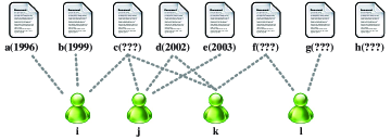
In this section, we move to the paper-author bipartite graph $G_{AP}$. An artificially created example of MYE problem in $G_{AP}$ is shown in Fig. 2. In this example, there are 8 papers ($a-h$) and 4 authors ($i-l)$, where papers $a,b,d,e$ have year information ($\in V_{P}^{K}$) while $c,f,g,h$ are missing year ($\in V_{P}^{U}$).

Figure 2: An example of a paper authorship network with 8 papers ($a-h$) and 4 authors ($i-l)$, where papers ($a,b,d,e$) are $\in V_{P}^{K}$ and ($c,f,g,h$) are $\in V_{P}^{U}$.

For $G_{AP}$, we will also introduce three algorithms, namely $G_{AP}$-Ba, $G_{AP}$-Iter and $G_{AP}$-AdvIter, in order of increasing complexity.

2.3.1 Algorithm for MYE in $G_{AP}$: $G_{AP}$-Ba and $G_{AP}$-Iter

$G_{AP}$-Ba is the basic algorithm and $G_{AP}$-Iter is simply repeating $G_{AP}$-Ba until convergence, thus we introduce them together. The basic algorithm, $G_{AP}$-Ba, consists of three steps:

1. Derive author’s active publishing window.

   For each author, based on the graph topology and paper year information, we can derive an active paper publishing window. Eqs. (10) and (11) give the definition of the two bounds of this window:

   $$AW\_Min(a)=\min_{p\in P(a)\cap V_{P}^{K}}Y(p),$$ (10)

   $$AW\_Max(a)=\max_{p\in P(a)\cap V_{P}^{K}}Y(p),$$ (11)

   where $P(a),\forall\;a\;\in V_{A}$ is the paper set written by author $a$. It is possible that $P(a)\cap V_{P}^{K}=\emptyset$, and we consider it as a non-existent bound. According to the above definition, the two bounds are either co-existent or non-existent.
   

2. Derive the paper’s possible year estimation window.

   Based on the derived author active window, we can further define the paper possible year window:

   $$\hat{Y}_{AMin}(p^{U})=\min\{\max_{a\in A(p^{U})}AW\_min(a),\min_{a\in A(p^{U})}AW\_max(a)\},$$ (12)

   $$\hat{Y}_{AMax}(p^{U})=\max\{\max_{a\in A(p^{U})}AW\_min(a),\min_{a\in A(p^{U})}AW\_max(a)\},$$ (13)

   where $A(p^{U}),\forall p^{U}\in V_{P}^{U}$ is the author set of paper $p^{U}$.
   

   In most cases, $\hat{Y}_{AMin}(p^{U})=\max_{a\in A(p^{U})}AW\_min(a)$ and $\hat{Y}_{AMax}(p^{U})=\min_{a\in A(p^{U})}AW\_max(a)$. However, in case of the condition that authors’ active windows have no intersection (this is possible because the author active window dose not take the missing year papers into account), we rewrite them as Eqs. (12)-(13). For example, we look at paper $c$ in Fig. 2. The author set of paper $c$ is $A(c)=\{i(1996,1999),j(2002,2003),k(2002,2002)\}$ with the author active windows inside parentheses. Then by definition we get $\max_{a\in A(c)}AW\_Min(a)=\max\{1996,2002,2002\}=2002$, while $\min_{a\in A(c)}AW\_Max(a)=\min\{1999,2003,2002\}=1999$. Therefore, according to Eqs. (12)-(13), we can derive the possible year estimation window of paper $c:[1999,2002]$.
   

3. Calculate year value.

   In this algorithm, we apply the simple year value calculation method, the same one as in the $G_{P}$-SS algorithm. There is only a small difference in that in $G_{P}$-SS, there are four types of the year estimation window, whereas in $G_{AP}$, there are only two possible types, both bounds exist (Type-1) or neither exists (Type-4). Therefore, the estimated year value is either $\frac{\hat{Y}_{AMin}(p^{U})+\hat{Y}_{AMax}(p^{U})}{2}$ or labeled as Uncovered.

Note the rationale of the design of the basic algorithm is based on an observation that most authors are continuously active in publishing papers. Hence, the publishing years of his/her papers are usually within a continuous window. If we obtain the windows of all the coauthors of a missing year paper, the intersection of these windows will be an interval that most probably contains the real publishing year.

Algorithm 3 The pseudo code of $G_{AP}$-Iter

1:  repeat

2:     for all $e=(a,p)\in E_{AP},a\in V_{A},p\in V_{P}$ do

3:        if $p\in V_{P}^{K}$ then

4:           $AW\_Min(a)\leftarrow\min\{Y(p),AW\_Min(a)\}$

5:           $AW\_Max(a)\leftarrow\max\{Y(p),AW\_Max(a)\}$

6:        else if $\hat{Y}(p)$ exists then /* $p\in V_{P}^{U}$ */

7:           $AW\_Min(a)\leftarrow\min\{\hat{Y}(p),AW\_Min(a)\}$

8:           $AW\_Max(a)\leftarrow\max\{\hat{Y}(p),AW\_Max(a)\}$

9:        end if

10:     end for

11:     for all $p^{U}\in V_{P}^{U}$ do

12:        for all $a\in A(p^{U})$ do

13:           $maxMin\leftarrow\max\{AW\_Min(a),maxMin\}$

14:           $minMax\leftarrow\min\{AW\_Max(a),minMax\}$

15:        end for

16:        $\hat{Y}_{AMin}(p^{U})\leftarrow\min\{maxMin,minMax\}$

17:        $\hat{Y}_{AMax}(p^{U})\leftarrow\max\{maxMin,minMax\}$

18:        $\hat{Y}(p^{U})\leftarrow\frac{\hat{Y}_{AMin}(p^{U})+\hat{Y}_{AMax}(p^{U})}{2}$

19:     end for

20:  until No update happens

The pseudo code for $G_{AP}$-Iter (including $G_{AP}$-Ba) is shown in Algorithm 3. Lines 2-19 are the steps of $G_{AP}$-Ba, $G_{AP}$-Iter is simply repeating $G_{AP}$-Ba (Line 1). The estimation results in the previous rounds affect the subsequent rounds because each author’s active publishing window will be re-calculated according to all the paper year information (given or estimated in the last round, Lines 7-8). Lines 13-17 are the implementation of Eqs. (12) and (13). The intermediate and final estimation results of running $G_{AP}$-Iter on the example in Fig. 2 is listed in Table 7.

Node	Type	Round 1	Round 2	Round 3
$i$	Author	$(1996,1999)$	$(1996,2001)$	$(1996,2001)$
$j$	Author	$(2002,2003)$	$(2001,2003)$	$(2001,2003)$
$k$	Author	$(2002,2002)$	$(2001,2002)$	$(2001,2002)$
$l$	Author	$(-\infty,+\infty)$	$(2002,2002)$	$(2002,2002)$
$c$	Paper	$(1999,2002)$	$(2001,2001)$	$(2001,2001)$
$\hat{Y}(c)$		2001 (2000.5)	2001	2001
$f$	Paper	$(2002,2002)$	$(2002,2002)$	$(2002,2002)$
$\hat{Y}(f)$		2002	2002	2002
$g$	Paper	$(-\infty,+\infty)$	$(2002,2002)$	$(2002,2002)$
$\hat{Y}(g)$		Uncovered	2002	2002
$h$	Paper	$(-\infty,+\infty)$	$(-\infty,+\infty)$	$(-\infty,+\infty)$
$\hat{Y}(h)$		Uncovered	Uncovered	Uncovered

Table 7: The intermediate and final estimation results obtained by running $G_{AP}$-Ba and $G_{AP}$-Iter on the example shown in Fig. 2

In Table 7, the $G_{AP}$-Iter repeats 3 rounds until convergence. We show the intermediate results of the author active windows for author (nodes $i,j,k,l$), the possible paper publishing windows for missing year papers (nodes $c,f,g,h$), and their estimation results ($\hat{Y}(p^{U}),p^{U}\in\{c,f,g,h\}$) in each round. The column labeled as “Round 1” shows the results generated by algorithm $G_{AP}$-Ba. Comparing to $G_{AP}$-Ba, $G_{AP}$-Iter helps to share information through the co-author relationships, like author $l$ in Table 7. Therefore, $G_{AP}$-Iter obtains a lower uncovered ratio (1/4) than $G_{AP}$-Ba (2/4).

We need to note that $G_{AP}$-Iter may add inaccuracy during the information propagation, i.e. the estimation results in the previous rounds affect the derivation of both the author active windows and estimation results in the subsequent rounds. For example, $\hat{Y}(c)$ after Round 1 is 2001. In Round 2, the active windows of all the coauthors of paper $c$, $P(c)=\{i,j,k\}$ are updated, and hence the related paper year estimation windows get updated also. Although $G_{AP}$-Iter helps to decrease the uncovered ratio, it may not improve an estimation accuracy like MAE (under certain situations, $G_{AP}$-Iter can be even worse than $G_{AP}$-Ba).

In order to compensate for the weakness of $G_{AP}$-Iter so that both the uncovered ratio and estimation accuracies are improved we propose the $G_{AP}$-AdvIter, which has an advanced iteration procedure to reduce the propagation of inaccurate information.

2.3.2 Algorithm for MYE in $G_{AP}$: $G_{AP}$-AdvIter

According to the previous discussion, the key point of improving the estimation accuracy in $G_{AP}$ is to propagate as much “good” information as possible. Hence, we propose a heuristic algorithm, $G_{AP}$-AdvIter to achieve this. Here are some definitions:

1. Consistent-Coauthor-Count between two papers: the number of common coauthors of the two papers. We denote it by function $w(\cdot)$. Given any two papers, we can calculate their Consistent-Coauthor-Count by the following expression:

   $$\forall\;p,\;q\;\in\;V_{P},\;w(p,q)=w(q,p)=|A(p)\cap A(q)|,$$ (14)

   where $w(\cdot)$ is a non-negative integer and equals to zero only when the two papers have no common coauthors.

2. $w$-Consistent-Coauthor-Pair relationship: if any two papers, $\forall p,q\in V_{P}$, satisfy: $w(p,q)=w(q,p)>1$, then we call them a $w$-Consistent-Coauthor-Pair.

3. Consistent-Coauthor-Pair set of a paper $p\in V_{P}$, denoted by $\Omega(p)$:

   $$\Omega(p)=\{q|q\in V_{P}\;\textrm{and}\;w(p,q)>1\}$$ (15)

We give some illustrations of these definitions using the example in Fig. 2: $w(a,g)=|\emptyset|=0$ and $w(c,d)=|\{j,k\}|=2$, thus, paper $c,d$ have the 2-Consistent-Coauthor-Pair relationship. Not including this, there are no more Consistent-Coauthor-Pairs in Fig. 2. Therefore, we obtain $\Omega(c)=\{d\}$, $\Omega(d)=\{c\}$ and $\Omega(p)=\emptyset,\forall p\in\{a,b,e,f,g,h\}$.

It is a reasonable assumption that if more authors work together and publish papers, it is more probable that these papers are published within a small time window. For example, students who worked together with their supervisors/group members and published certain papers during their Master/PhD study. Note this is only a sufficient condition, the reverse may not be true.

The above assumption implies that if two papers have a $w$-Consistent-Coauthor-Pair relationship, then there is a high probability that their publishing years are close. In addition, this probability is positively correlated to the value of $w$. We conjecture that the estimated year values from utilizing the $w$-Consistent-Coauthor-Pair relationship must be “better” information for propagation.

The pseudo code of $G_{AP}$-AdvIter is listed in Algorithm 4, which shows how we make use of the more reliable information for propagation.

Algorithm 4 The pseudo code of $G_{AP}$-AdvIter

1:  for all $p^{U}\in V_{P}^{U}$ do

2:     Derive the Consistent-Coauthor-Pair set, $\Omega(p^{U})$.

3:  end for

4:  repeat

5:     for all $e=(a,p)\in E_{AP},a\;\in V_{A},p\in V_{P}$ do

6:        if $p\in V_{P}^{K}$ then

7:           $AW\_Min(a)\leftarrow\min\{Y(p),AW\_Min(a)\}$

8:           $AW\_Max(a)\leftarrow\max\{Y(p),AW\_Max(a)\}$

9:        else if $\hat{Y}(p)$ exists then /* $p\in V_{P}^{U}$ */

10:           $AW\_Min(a)\leftarrow\min\{\hat{Y}(p),AW\_Min(a)\}$

11:           $AW\_Max(a)\leftarrow\max\{\hat{Y}(p),AW\_Max(a)\}$

12:        end if

13:     end for

14:     for all $p^{U}\in V_{P}^{U}$ do

15:        if $\Omega(p^{U})\cap V_{P}^{K}\neq\emptyset$ then /* for AdvIter */

16:           $\hat{Y}(p^{U})\leftarrow W(p^{U},\gamma)$

17:        else

18:           for all $a\in A(p^{U})$ do

19:              $maxMin\leftarrow\max\{AW\_Min(a),maxMin\}$

20:              $minMax\leftarrow\min\{AW\_Max(a),minMax\}$

21:           end for

22:           $\hat{Y}_{AMin}(p^{U})\leftarrow\min\{maxMin,minMax\}$

23:           $\hat{Y}_{AMax}(p^{U})\leftarrow\max\{maxMin,minMax\}$

24:           $\hat{Y}(p^{U})\leftarrow\frac{\hat{Y}_{AMin}(p^{U})+\hat{Y}_{AMax}(p^{U})}{2}$

25:        end if

26:     end for

27:  until No update happens

Comparing to Algorithm 3, we notice that Algorithm 4 only added Lines 1-3 and Lines 15-16. Lines 1-3 is the process used to find $\Omega(p^{U})$ for each missing year paper, this is done during initialization. Lines 15-16 show that we give higher priority to estimating year values if the $w$-Consistent-Coauthor-Pair relationship can help, than the basic procedure (Lines 17-25). The expression of the function $W$ is in Eq. (16):

$$W(p^{U},\gamma)=\frac{\sum_{q\in\Omega(p^{U})\cap V_{P}^{K}}\;\;w(p^{U},q)^{\gamma}\times Y(q)}{\sum_{q\in\Omega(p^{U})\cap V_{P}^{K}}w(p^{U},q)^{\gamma}},\quad\textrm{if}\;\Omega(p^{U})\cap V_{P}^{K}\neq\emptyset$$ (16)

The meaning of Eq. (16) is to take a $\gamma$-weighted average on the given year information of those papers in the set $\Omega(p^{U})\cap V_{P}^{K}$. For example, if $\Omega(p^{U})\cap V_{P}^{K}=\{q,r\},w(p^{U},q)=2,w(p^{U},r)=3,Y(q)=2000,Y(r)=2002$, then $W(p^{U},\gamma)=\frac{2^{\gamma}\times 2000+3^{\gamma}\times 2002}{2^{\gamma}+3^{\gamma}}$. Here parameter $\gamma$ is used to tune the importance we put on the values of $w$, e.g., if we set $\gamma=0$, it implies that no weight is considered and the result is simply the average. When $\gamma=1$, it is a normal weighted average calculation; while when $\gamma\rightarrow\infty$, it leads to the special case where only the papers in the set $\Omega(p^{U})\cap V_{P}^{K}$ with the largest $w$ are involved in the calculation. In addition, since it is meaningless for function $W$ if $\Omega(p^{U})\cap V_{P}^{K}=\emptyset$, we need to check beforehand (Line 15).

Node	Type	Round 1	Round 2	Round 3
$i$	Author	$(1996,1999)$	$(1996,2002)$	$(1996,2002)$
$j$	Author	$(2002,2003)$	$(2002,2003)$	$(2002,2003)$
$k$	Author	$(2002,2002)$	$(2002,2002)$	$(2002,2002)$
$l$	Author	$(-\infty,+\infty)$	$(2002,2002)$	$(2002,2002)$
$c$	Paper	$(2002,1999)$	$(2001,2001)$	$(2001,2001)$
$\hat{Y}(c)$	$W(c,0)$	2002	2002	2002
$f$	Paper	$(2002,2002)$	$(2002,2002)$	$(2002,2002)$
$\hat{Y}(f)$		2002	2002	2002
$g$	Paper	$(-\infty,+\infty)$	$(2002,2002)$	$(2002,2002)$
$\hat{Y}(g)$		Uncovered	2002	2002
$h$	Paper	$(-\infty,+\infty)$	$(-\infty,+\infty)$	$(-\infty,+\infty)$
$\hat{Y}(h)$		Uncovered	Uncovered	Uncovered

Table 8: The intermediate and final estimation results obtained by running $G_{AP}$-AdvIter on the example shown in Fig. 2

In Table 8, we list the intermediate and final estimation results obtained by running $G_{AP}$-AdvIter on the example shown in Fig. 2. As analyzed previously, $\Omega(c)=\{d\}$, $\Omega(d)=\{c\}$ and $\Omega(p)=\emptyset,\forall p\in\{a,b,e,f,g,h\}$, hence only $\hat{Y}(c)=Y(d)=2002$ is affected by $G_{AP}$-AdvIter and also the related author active windows: $i:(1996,2002)$, $j:(2002,2003)$ and $k:(2002,2002)$.

2.4 MYE for heterogenous network $G$

For a heterogeneous network, $G=(G_{P}\cup G_{AP})$, which consists of both $G_{P}$ and $G_{AP}$, we make use of the proposed methods and the results discussed in the previous two sections. Since for both $G_{P}$ and $G_{AP}$, we proposed three algorithms of different complexity, there can be altogether 9 different combinations. With careful consideration, we pick out 3 typical combinations as MYE algorithms for $G$:

1. $G$-SSBa: combination of $G_{P}$-SS and $G_{AP}$-Ba

2. $G$-ASIter: combination of $G_{P}$-AS and $G_{AP}$-Iter

3. $G$-AdvIter: combination $G_{P}$-AA and $G_{AP}$-AdvIter

In fact, selecting the “combination” is not trivial, this will be explained in more detail next. The common part of the two algorithms consists of these two steps: (a) derivation of possible year estimation window and (b) calculate the estimated year value based on the derived window.

No matter which combined algorithm for $G$ is applied, for each missing year paper, two possible year estimation windows will be derived, one by the $G_{P}$ part $[\hat{Y}_{CMin}(p^{U}),\hat{Y}_{CMax}(p^{U})]$, and the other by the $G_{AP}$ part $[\hat{Y}_{AMin}(p^{U}),\hat{Y}_{AMax}(p^{U})]$, due to the independency of the two procedures.

Considering the four types of the derived estimation window from $G_{P}$ and two types from $G_{AP}$, each missing year paper can end with the following four cases of which case (d) is most likely:

1. $(\hat{Y}_{CMin}(p^{U}),\hat{Y}_{CMax}(p^{U}))=(\hat{Y}_{AMin}(p^{U}),\hat{Y}_{AMax}(p^{U}))=(-\infty,+\infty)$, then it can only lead to the Uncovered estimation result;

2. $(\hat{Y}_{CMin}(p^{U}),\hat{Y}_{CMax}(p^{U}))=(-\infty,+\infty)$ but $[\hat{Y}_{AMin}(p^{U}),\hat{Y}_{AMax}(p^{U})]$ is not, then it is as if only the $G_{AP}$ part algorithm is in action;

3. $(\hat{Y}_{AMin}(p^{U}),\hat{Y}_{AMax}(p^{U}))=(-\infty,+\infty)$ but $[\hat{Y}_{CMin}(p^{U}),\hat{Y}_{CMax}(p^{U})]$ is not, then it is as if only the $G_{P}$ part algorithm is in action;

4. Neither window is $(-\infty,+\infty)$, we will have a detailed discussion for the three algorithms: $G$-SSBa, $G$-ASIter and $G$-AdvIter respectively.

A general criterion is used to combine $G$-SSBa, $G$-ASIter and $G$-AdvIter, this criterion is that we always give higher priority to the window derived from $G_{P}$ than from $G_{AP}$. This is because the former is more reliable than the latter, as the latter may involve inaccuracy in information propagation.

2.4.1 Algorithm for MYE in $G$: $G$-SSBa and $G$-ASIter

Since the structures of $G$-SSBa and $G$-ASIter are similar, we try to merge their pseudo codes together for space saving and ease of description. The pseudo code of $G$-SSBa and $G$-ASIter for case (d) is listed in Algorithm 5.

Algorithm 5 The pseudo code of $G$-SSBa and $G$-ASIter for case (d)

1:  if $G$-SSBa then

2:     $[\hat{Y}_{CMin},\hat{Y}_{CMax}]\leftarrow$ Simple Window Derivation Method in Eq. (2) and (3);

3:  else if $G$-ASIter then

4:     $[\hat{Y}_{CMin},\hat{Y}_{CMax}]\leftarrow$ Advanced Window Derivation Method in Algorithm 1;

5:  end if

6:  repeat

7:     $[\hat{Y}_{AMin},\hat{Y}_{AMax}]\leftarrow$ by $G_{AP}$-Ba, Eqs. (10), (11), (12), (13);

8:     for all $p^{U}\in V_{P}^{U}$ do

9:        /* Init */

10:        $\hat{Y}_{GMin}(p^{U})\leftarrow-\infty$;

11:        $\hat{Y}_{GMax}(p^{U})\leftarrow+\infty$;

12:        if $\hat{Y}_{CMin}(p^{U})>-\infty$ and $\hat{Y}_{CMax}(p^{U})<+\infty$ then

13:           /* Type-1 Window in $G_{P}$ */

14:           if $\hat{Y}_{AMin}(p^{U})<\hat{Y}_{CMin}(p^{U})$ or $\hat{Y}_{AMax}(p^{U})>\hat{Y}_{CMax}(p^{U})$ then

15:              $\hat{Y}_{GMin}(p^{U})\leftarrow\hat{Y}_{CMin}(p^{U})$;

16:              $\hat{Y}_{GMax}(p^{U})\leftarrow\hat{Y}_{CMax}(p^{U})$;

17:           else

18:              $\hat{Y}_{GMin}(p^{U})\leftarrow\max\{\hat{Y}_{CMin}(p^{U}),\hat{Y}_{AMin}(p^{U})\}$;

19:              $\hat{Y}_{GMax}(p^{U})\leftarrow\min\{\hat{Y}_{CMax}(p^{U}),\hat{Y}_{AMax}(p^{U})\}$;

20:           end if

21:        else if $\hat{Y}_{CMin}(p^{U})>-\infty$ and $\hat{Y}_{CMax}(p^{U})=+\infty$ then

22:           /* Type-2 Window in $G_{P}$ */

23:           if $\hat{Y}_{AMax}(p^{U})<\hat{Y}_{CMin}(p^{U})$ then

24:              $\hat{Y}_{GMin}(p^{U})\leftarrow\hat{Y}_{CMin}(p^{U})$;

25:              $\hat{Y}_{GMax}(p^{U})\leftarrow\hat{Y}_{CMin}(p^{U})$;

26:           else

27:              $\hat{Y}_{GMin}(p^{U})\leftarrow\max\{\hat{Y}_{CMin}(p^{U}),\hat{Y}_{AMin}(p^{U})\}$;

28:              $\hat{Y}_{GMax}(p^{U})\leftarrow\hat{Y}_{AMax}(p^{U})$;

29:           end if

30:        else if $\hat{Y}_{CMin}(p^{U})=-\infty$ and $\hat{Y}_{CMax}(p^{U})<+\infty$ then

31:           /* Type-3 Window in $G_{P}$ */

32:           if $\hat{Y}_{AMin}(p^{U})>\hat{Y}_{CMax}(p^{U})$ then

33:              $\hat{Y}_{GMin}(p^{U})\leftarrow\hat{Y}_{CMax}(p^{U})$;

34:              $\hat{Y}_{GMax}(p^{U})\leftarrow\hat{Y}_{CMax}(p^{U})$;

35:           else

36:              $\hat{Y}_{GMin}(p^{U})\leftarrow\hat{Y}_{AMin}(p^{U})$;

37:              $\hat{Y}_{GMax}(p^{U})\leftarrow\min\{\hat{Y}_{CMax}(p^{U}),\hat{Y}_{AMax}(p^{U})\}$;

38:           end if

39:        else

40:           /* Type-4 Window in $G_{P}$ */

41:           Case (b);

42:        end if

43:        /* Simple Year Value Calculation */

44:        $\hat{Y}(p^{U})\leftarrow\frac{\hat{Y}_{GMin}(p^{U})+\hat{Y}_{GMax}(p^{U})}{2}$;

45:     end for

46:     if $G$-SSBa then

47:        Break;

48:     end if

49:  until No update happens

In Algorithm 5, we denote $\hat{Y}_{GMin}(p^{U}),\hat{Y}_{GMax}(p^{U})$ to be the two bounds of the derived year estimation window in $G$. In the beginning, we derive $[\hat{Y}_{CMin},\hat{Y}_{CMax}]$ by a simple window derivation method for algorithm $G$-SSBa, or an advanced window derivation method for algorithm $G$-ASIter (Lines 1-5).

Next, we derive $[\hat{Y}_{GMin},\hat{Y}_{GMax}]$ depending on the type of the window in $G_{P}$, e.g., Lines 12-20 for Type-1, Lines 21-29 for Type-2 and Lines 30-38 for Type-3. The derivation follows the general criterion that if the intersection of $[\hat{Y}_{CMin}(p^{U}),\hat{Y}_{CMax}(p^{U})]$ and $[\hat{Y}_{AMin}(p^{U}),\hat{Y}_{AMax}(p^{U})]$ is not empty, we take this intersection window as $[\hat{Y}_{GMin}(p^{U}),\hat{Y}_{GMax}(p^{U})]$; otherwise, we take $[\hat{Y}_{CMin}(p^{U}),\hat{Y}_{CMax}(p^{U})]$. Line 44 is the same simple year value calculation method as in $G_{P}$-SS, $G_{P}$-AS, $G_{AP}$-Ba and $G_{AP}$-Iter. In fact, if conditions (Line 23 or Line 32) happen (i.e. the two windows do not intersect with each other), the operation (Lines 24-25 and Lines 33-34, together Line 44) is equivalent to Eq. (5)-Eq. (6), taking the bound values. For $G$-SSBa of which the combination includes $G_{AP}$-Ba, the basic procedure will only be carried out once (Lines 46-48); While for $G$-ASIter of which the combination includes $G_{AP}$-Iter, the $[\hat{Y}_{GMin},\hat{Y}_{GMax}]$ window will be propagated until convergence (Line 6 together with Line 49).

2.4.2 Algorithm for MYE in $G$: $G$-AdvIter

$G$-AdvIter is the combination of $G_{P}$-AA and $G_{AP}$-AdvIter, therefore, the concepts of training set $\mathcal{T}$ as well as the Consistent-Coauthor-Pair relationship will be involved. Algorithm 6 list the pseudo code of $G$-AdvIter for case (d):

Algorithm 6 The pseudo code of $G$-AdvIter for case (d)

1:  Run Algorithm 2, derive $[\hat{Y}_{CMin},\hat{Y}_{CMax}]$ and the training set $\mathcal{T}$.

2:  for all $p^{U}\in V_{P}^{U}$ do

3:     Derive the Consistent-Coauthor-Pair set, $\Omega(p^{U})$.

4:  end for

5:  repeat

6:     $[\hat{Y}_{AMin},\hat{Y}_{AMax}]\leftarrow$ by $G_{AP}$-Ba, Eqs. (10), (11), (12), (13);

7:     for all $p^{U}\in V_{P}^{U}$ do

8:        $\hat{Y}(p^{U})\leftarrow Null$;

9:        if $\hat{Y}_{CMin}(p^{U})>-\infty$ and $\hat{Y}_{CMax}(p^{U})<+\infty$ then

10:           /* Type-1 Window in $G_{P}$ */

11:           Derivation of $\hat{Y}_{GMin}(p^{U}),\hat{Y}_{GMax}(p^{U})$; /* Same as Algorithm 5, Lines 12-20 */

12:           /* Year Value Calculate */

13:           if $\Omega(p^{U})\cap V_{P}^{K}\neq\emptyset$ then

14:              $\hat{Y}(p^{U})\leftarrow W_{G}(p^{U},\gamma,\hat{Y}_{CMin}(p^{U}),\hat{Y}_{CMax}(p^{U}))$

15:           end if

16:           if $\hat{Y}(p^{U})=Null$ then /* In case $W_{G}$ does not work */

17:              $\hat{Y}(p^{U})\leftarrow\frac{\hat{Y}_{GMin}(p^{U})+\hat{Y}_{GMax}(p^{U})}{2}$;

18:           end if

19:        else if $\hat{Y}_{CMin}(p^{U})>-\infty$ and $\hat{Y}_{CMax}(p^{U})=+\infty$ then

20:           /* Type-2 Window in $G_{P}$ */

21:           Derivation of $\hat{Y}_{GMin}(p^{U}),\hat{Y}_{GMax}(p^{U})$; /* Same as Algorithm 5, Lines 21-29 */

22:           /* Year Value Calculate */

23:           $dResult\leftarrow d(\textrm{Type-2},\hat{Y}_{CMin}(p^{U}))$;/*call $d(WinType(p^{U}),BoundVal(p^{U})$*/

24:           $\delta\leftarrow dResult-\hat{Y}_{CMin}(p^{U})$;

25:           if $\Omega(p^{U})\cap V_{P}^{K}\neq\emptyset$ then

26:              $\hat{Y}(p^{U})\leftarrow W_{G}(p^{U},\gamma,\hat{Y}_{CMin}(p^{U}),\hat{Y}_{CMin}(p^{U})+2\delta)$

27:           end if

28:           if $\hat{Y}(p^{U})=Null$ then /* In case $W_{G}$ does not work */

29:              if $\hat{Y}_{AMax}(p^{U})<\hat{Y}_{CMin}(p^{U})$ or $dResult\in(\hat{Y}_{GMin}(p^{U}),\hat{Y}_{GMax}(p^{U}))$ then

30:                 $\hat{Y}(p^{U})\leftarrow dResult$

31:              else

32:                 $\hat{Y}(p^{U})\leftarrow\frac{\hat{Y}_{GMin}(p^{U})+\hat{Y}_{GMax}(p^{U})}{2}$;

33:              end if

34:           end if

35:        else if $\hat{Y}_{CMin}(p^{U})=-\infty$ and $\hat{Y}_{CMax}(p^{U})<+\infty$ then

36:           /* Type-3 Window in $G_{P}$ */

37:           Derivation of $\hat{Y}_{GMin}(p^{U}),\hat{Y}_{GMax}(p^{U})$; /* Same as Algorithm 5, Lines 30-38 */

38:           /* Year Value Calculate */

39:           $dResult\leftarrow d(\textrm{Type-3},\hat{Y}_{CMax}(p^{U}))$;/*call $d(WinType(p^{U}),BoundValue(p^{U})$*/

40:           $\delta\leftarrow\hat{Y}_{CMax}(p^{U})-dResult$;

41:           if $\Omega(p^{U})\cap V_{P}^{K}\neq\emptyset$ then

42:              $\hat{Y}(p^{U})\leftarrow W_{G}(p^{U},\gamma,\hat{Y}_{CMax}(p^{U})-2\delta,\hat{Y}_{CMax}(p^{U}))$

43:           end if

44:           if $\hat{Y}(p^{U})=Null$ then /* In case $W_{G}$ does not work */

45:              if $\hat{Y}_{AMin}(p^{U})>\hat{Y}_{CMax}(p^{U})$ or $dResult\in(\hat{Y}_{GMin}(p^{U}),\hat{Y}_{GMax}(p^{U}))$ then

46:                 $\hat{Y}(p^{U})\leftarrow dResult$

47:              else

48:                 $\hat{Y}(p^{U})\leftarrow\frac{\hat{Y}_{GMin}(p^{U})+\hat{Y}_{GMax}(p^{U})}{2}$;

49:              end if

50:           end if

51:        else

52:           /* Type-4 Window in $G_{P}$: Case (b); */

53:        end if

54:     end for

55:  until No update happens

In Algorithm 6, we omit the same code of deriving $\hat{Y}_{GMin}(p^{U}),\hat{Y}_{GMax}(p^{U})$ as in Algorithm 5 (Lines 11, 21, 37). At the beginning (Line 1), we call the function $G_{P}$-AA (Algorithm 2) to derive $\hat{Y}_{CMin}(p^{U}),\hat{Y}_{CMax}(p^{U})$ and the training set $\mathcal{T}$, which is a series of 3-tuple data $\{y_{t},WinType_{t},BoundVal_{t}\}$ from the papers with known year information. The preparation of the Consistent-Coauthor-Pair set for each missing year paper $\Omega(p^{U})$, like $G_{AP}$-AdvIter, is also called (Lines 2-4). The main difference between $G$-AdvIter and $G$-ASIter is the method of calculating year value. For all three types of window in $G_{P}$, we apply the $W_{G}(p^{U},\gamma,y_{l},y_{r})$ function to calculate the year value:

$$\textrm{When}\;\Omega_{G}(p^{U}) = \{q|q\in\Omega(p^{U}),Y(q)\in(y_{l},y_{r})\},\textrm{and}\;\Omega_{G}(p^{U})\cap V_{P}^{K}\neq\emptyset,$$

$$W_{G}(p^{U},\gamma,y_{l},y_{r}) = \frac{\sum_{q\in\Omega_{G}(p^{U})\cap V_{P}^{K}}\;\;w(p^{U},q)^{\gamma}\times Y(q)}{\sum_{q\in\Omega_{G}(p^{U})\cap V_{P}^{K}}w(p^{U},q)^{\gamma}};$$

Otherwise $$= Null.$$ (17)

In Eq. (17), the different part of $W_{G}$ is that we pick out a subset of papers from $\Omega(p^{U})$, denoted by $\Omega_{G}(p^{U})$, satisfying the condition that the paper publishing years are within an input window $[y_{l},y_{r}]$, i.e., $\Omega_{G}(p^{U})=\{q|q\in\Omega(p^{U}),Y(q)\in[y_{l},y_{r}]\}$. For Type-1 window of $G_{P}$, we choose the subset $\Omega_{G}(p^{U})$ by setting the input window to be $[y_{l}=\hat{Y}_{CMin}(p^{U}),y_{r}=\hat{Y}_{CMax}(p^{U})]$ for calculating $\hat{Y}(p^{U})$ (Line 14). But if $\Omega_{G}(p^{U})\cap V_{P}^{K}=\emptyset$, we revert back to the default way (Lines 16-18).

The process for a Type-2 or Type-3 window is a little more complicated. For a Type-2 window, both $\Omega(p^{U})$ and $\mathcal{T}$ are available tools. Due to this we propose the following way: we first derive the estimation year value, denoted by $dResult$, through $d(\cdot)$ function expressed in Eq. (9). We use this $dResult$ and the input parameter $\hat{Y}_{CMin}(p^{U})$ to define a window [$y_{l}=\hat{Y}_{CMin}(p^{U})$, $y_{r}=\hat{Y}_{CMin}(p^{U})+2\delta]$, of which the interval equals to twice of the distance from $dResult$ to $\hat{Y}_{CMin}(p^{U})$, $\delta=dResult-\hat{Y}_{CMin}(p^{U})$. This window is then used to derive $\Omega_{G}(p^{U})$ and calculate $\hat{Y}(p^{U})$ (Lines 23-27). If $\Omega_{G}(p^{U})\cap V_{P}^{K}=\emptyset$, we have a second choice which is $dResult$, if one of the following two conditions is met: (a) The two windows $[\hat{Y}_{CMin}(p^{U}),\hat{Y}_{CMax}(p^{U})]$ and $[\hat{Y}_{AMin}(p^{U}),\hat{Y}_{AMax}(p^{U})]$ have no intersection; or (b) $dResult\in[\hat{Y}_{GMin}(p^{U}),\hat{Y}_{GMax}(p^{U})]$ (Lines 28-31). Otherwise, we change back to the default way (Line 32).

The process for a Type-3 window is symmetric to Type-2. The only difference is that the input window for deriving $\Omega_{G}(p^{U})$ and $\hat{Y}_{CMin}(p^{U})$ becomes $W_{G}(p^{U},\gamma,y_{l}=\hat{Y}_{CMax}(p^{U})-2\delta,y_{r}=\hat{Y}_{CMax}(p^{U}))$ (Lines 39-43).

3 Experiment Results

In this section we present the experiment settings and evaluation results. In the experiment, we test the proposed MYE algorithms in the last section by applying them to all the three types of the academic social networks, the paper citation network $G_{P}$, the paper authorship network $G_{AP}$ and the heterogenous network $G$.

3.1 Data Sets

We have tried three different data sets: Microsoft academic data set Libra (2013), DBLP Ley (2009) with additional citation information, DBLP-Cit data set Tang et al (2007, 2008), and American Physical Society data set APS (2013). The raw data sets are not perfect in that: (a) there exits a proportion of missing year papers; (b) Some citation links are pointing from early published papers to later ones, which breaks Assumption 1.

Since the performance evaluation needs ground truth knowledge, we have to do some preprocessing on the original data sets, including: a) remove these missing year papers and their relationships (citation links and paper-authorship links); b) remove those citation links that break Assumption 1.

Table 9 lists the general information about the three data sets after preprocessing:

Data set	Microsoft Libra	DBLP-Cit	APS
Input Window	(1900 - 2013)	(1900 - 2013)	(1900 - 2013)
#papers	2323235	1558503	463347
#authors	1278407	914053	320964
#total citation links	10003121	2062896	4689142

Table 9: General information of the three data sets used after preprocessing.

As we can see in Table 9, the average number of citation links per paper of the three data sets are: 4.31 for Libra, 1.33 for DBLP-Cit and 10.34 for APS, which appears disparate. This probably reflects how well these three data sets are collected and managed. The APS data set is the most complete in terms of the paper citation information, and the DBLP-Cit is probably the least. For DBLP-Cit, the job to find citation links for an existing paper set is a big challenge. The small number of average paper citation links shows that it is likely only a small proportion of the complete paper citation links are found.

The completeness and accuracy of the citation links will only affect those MYE algorithms that rely on citation information, e.g., the three algorithms for $G_{P}$.

3.2 Evaluation methodology

We apply a similar approach to the K-fold cross validation method Mosteller and Tukey (1968); Kohavi (1995) to evaluate the MYE algorithms. For each date set after pre-processing, we randomly split the paper set into $K$ mutually exclusive groups, i.e., $V_{P}=\bigcup_{k=1}^{K}V_{P_{k}},\textrm{and}\;\forall i\neq j,V_{P_{i}}\cap V_{P_{j}}=\emptyset$. In addition, each group has approximately the same size, $|V_{P_{k}}|\approx\frac{|V_{P}|}{K},k=1,2,\dots,K$.

For a given parameter $K$, the experiment repeats $K$ times. In the $j$th time, the year information of the papers in group $V_{P_{j}}$ is artificially hidden, thus assumed to be the missing year paper set $V_{P}^{U}=V_{P_{j}}$, and the remaining groups become the paper set with known year information, i.e., $V_{P}^{K}=V_{P}\setminus V_{P_{j}}$. The overall performance metrics take the average of the results obtained in each of the $K$ times.

Indirectly, the value of $K$ controls the severity of the missing year phenomenon. For convenience, we define $\eta=\frac{|V_{P}^{U}|}{|V_{P}|}\approx\frac{1}{K}$ to be the Missing Year Ratio of the data set. Throughout the experiment, we have tried 5 different $\eta=\frac{1}{8},\frac{1}{5},\frac{1}{4},\frac{1}{3},\frac{1}{2}$.

3.3 Performance metrics

Three metrics are used to evaluate the performance of the MYE algorithms.

1. Coverage

   We have defined the uncovered ratio in Section 2. It equals to the number of those missing year papers finally labeled as Uncovered by MYE algorithms, divided by the total number of missing year papers $|V_{P}^{U}|$. We use $N^{U}=|V_{P}^{U}|-\textrm{Total\#Uncovered}$ to denote the number of the covered part. In one experiment, the coverage metric is equal to $\frac{N^{U}}{|V_{P}^{U}|}$. With K-fold cross validation, the overall coverage becomes:

   $$Coverage=\frac{1}{K}\sum_{k=1}^{K}\frac{N^{U}_{k}}{|V_{P_{k}}|},$$ (18)

   where the subscript $k$ indicates the $k$th iteration and $V_{P}^{U}=V_{P_{k}}$.

2. Mean absolute error (MAE)

   $$MAE=\frac{1}{K}\sum_{k=1}^{K}\bigg{(}\frac{1}{N^{U}_{k}}\sum_{i=1}^{N^{U}_{k}}|Y(p^{U}_{i})-\hat{Y}(p^{U}_{i})|\bigg{)},$$ (19)

   where the $k$th iteration, $V_{P}^{U}=V_{P_{k}}$, $\hat{Y}(p^{U}_{i})$ is the estimated year. $Y(p^{U}_{i})$ is the real year of $p^{U}_{i}$, which we assumed to be unknown when running the MYE algorithms and used only for validation purposes.

3. Root mean square error (RMSE)

   $$RMSE=\frac{1}{K}\sum_{k=1}^{K}\bigg{(}\sqrt{\frac{1}{N^{U}_{k}}\sum_{i=1}^{N^{U}_{k}}\big{[}Y(p^{U}_{i})-\hat{Y}(p^{U}_{i})\big{]}^{2}}\;\;\bigg{)}.$$ (20)

In order to have a better understanding of the coverage metric, we propose an analytical model to calculate the expected coverage for an undirected graph $G=(V,E)$. According to the basic graph theory Easley and Kleinberg (2010), $G$ can be partitioned into $S$ connected components $G=\bigcup_{i=1}^{S}G_{i}$, where $\forall i,j,G_{i}\cap G_{j}=\emptyset$.

The iteration mechanism of the MYE algorithms (e.g., $G_{AP}$-Iter, or $G_{AP}$-AdvIter) ensures that there can be only two possible outcomes for any connected component $G_{i}=(V_{i},E_{i})$ when propagation stops:

(I) All the missing year papers in this component have feasible estimated values (hence, $\neq$ Uncovered), if and only if there exits at least one paper with known year information in this component, i.e., $V_{i}\cap V_{P}^{K}\neq\emptyset$;

(II) Otherwise, all the missing year papers in this component are labeled as Uncovered.

If we assume the missing year paper is uniformly distributed among the whole paper set, then the expected coverage value can be calculated by Eq. (21):

$$Coverage\big{(}\eta,\bigcup_{i=1}^{S}V_{i}\big{)}=1-\frac{\sum_{i=1}^{S}\;\eta^{|V_{i}|}\cdot|V_{i}|}{\eta|V|}\;.$$ (21)

In Eq. (21), there are two inputs for this calculation: the year missing ratio $\eta$ and the vertex partition $V=\bigcup_{i=1}^{S}V_{i}$. According to the uniform distribution assumption, each paper is selected to be the missing year paper with equal probability $\eta$. Thus the denominator equals to the expected number of missing year papers $|V_{P}^{U}|=\eta|V|$. For each component $G_{i}$, $\eta^{|V_{i}|}$ is the probability that all the papers in it are missing year papers and $\eta^{|V_{i}|}\cdot|V_{i}|$ is hence the expected number of papers that will be labeled as Uncovered.

For the three types of the academic social networks, the above model actually cannot be applied directly. To apply it, we have to make proper modifications: (1) based on the citation network $G_{P}=(V_{P},E_{P})$, we construct $G_{P}^{\prime}=(V_{P},E_{P}^{\prime})$ by implicitly considering all the citation edges as undirected edges, where $E_{P}^{\prime}$ is the undirected edge set. (2) based on the paper authorship network $G_{AP}=(V_{A}\cup V_{P},E_{AP})$, we build a coauthor indicator graph $G_{AP}^{\prime}=(V_{P},E_{PP})$, where the existence of an edge between two papers in $G_{AP}^{\prime}$ indicates that they have at least one common author, i.e., $\forall e_{i,j}\in E_{PP},i,j\in V_{P}\Leftrightarrow A(i)\cap A(j)\neq\emptyset$, where $A(i)$ is the author set of paper $i$. (3) For the heterogenous network $G$, by simply combining $G_{P}^{\prime}$ and $G_{AP}^{\prime}$, we obtain $G^{\prime}=(V_{P},E_{P}^{\prime}\cup E_{PP})$. Now the analytical model can be applied on $G_{P}^{\prime}$, $G_{AP}^{\prime}$ and $G^{\prime}$ to calculate the expected coverage.

3.4 Experiment results in the citation network $G_{P}$

The first set of experiments are conducted on the citation network $G_{P}=(V_{P},E_{P})$. The coverage, MAE and RMSE results of algorithms $G_{P}$-SS, $G_{P}$-AS and $G_{P}$-AA are plotted in Figure 3.

(a) Coverage-Libra

(b) Coverage-DBLP

(c) Coverage-APS

(d) MAE-Libra

(e) MAE-DBLP

(f) MAE-APS

(g) RMSE-Libra

(h) RMSE-DBLP

(i) RMSE-APS

Figure 3: The Coverage, MAE and RMSE of algorithms $G_{P}$-SS (Simple Window Derivation and Simple Value Calculation), $G_{P}$-AS (Advanced Window Derivation and Simple Value Calculation) and $G_{P}$-AA (Advanced Window Derivation and Advanced Value Calculation) in a paper citation network $G_{P}$ of three data sets

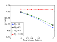
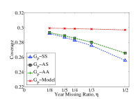
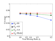
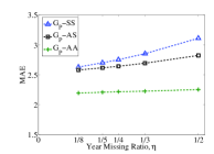
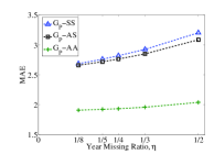
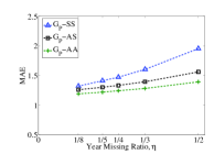
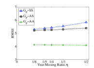
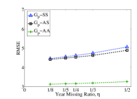
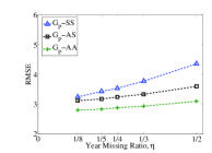
As shown in Figure 3, we have the following observations:

1. For all the three algorithms, when $\eta$ increases, coverage decreases while both MAE and RMSE increase. This implies the more information available helps to get better estimation results, more coverage and less estimation error.

2. In Fig. 3(a)-3(c), the curve of $G_{P}$-AS overlaps with that of $G_{P}$-AA and they have better coverage than $G_{P}$-SS. This is consistent with what we have discussed in Section 2 ($G_{P}$-AS and $G_{P}$-AA use the same advanced window derivation method). However, it appears that all the three coverage curves have certain deviation from the curve (with nodes of red “X” in Fig. 3(a)-3(c)) obtained by the analytical model in Eq. (21).
   
   The reason for this is that the analytical model overestimates the number of covered papers for $G_{P}$-AS and $G_{P}$-AA. Recall that in Section 2, the window propagation method in $G_{P}$ is different to the iteration scheme of $G_{AP}-Iter$ and $G_{AP}-AdvIter$ in that it follows the bound transmission rules in Eq. (8) and does not utilize estimation results in the previous rounds. As a result, the outcome (I) discussed above may not always be true, while (II) remains true. We use a typical and simple example to illustrate. As shown in Fig. 4, there are three papers ($a$, $b$, $c$) and two citation links, where only one paper $b$ has year information while the other two are missing year papers. Fig. 4 plots all the 7 possible topologies.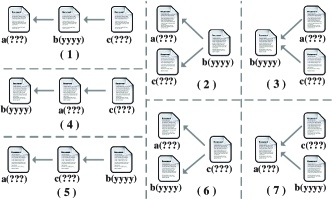

   

   Figure 4: An example of paper citation network with three papers ($a,b,c$) and two citation links. When two papers are missing year ($a$ and $c$), there are totally 7 possible topologies.

   According to outcome (I) of the analytical model, neither $a$ nor $c$ will be labeled as Uncovered. However, in Fig. 4 paper $a$ in case (6), and paper $c$ in case (7) get an Uncovered result by applying the advanced window derivation method in Eq. (8). This would build a more precise analytical model for the citation network, however this is too complicated. Therefore, we stick to the current method in Eq. (21) as an upper bound for the coverage achieved in citation network $G_{P}$.

3. $G_{P}$-AA outperforms the other two for all network types and data sets in terms of both coverage and estimation accuracy, MAE and RMSE.

4. Comparing the three data sets, we find that the coverage on APS data is much higher than the other two and DBLP-Cit is the lowest. This is mainly caused by the completeness of the citation information of the three data sets, mentioned in the beginning of this section. Since APS maintains very complete and accurate citation information, this benefits both coverage and accuracy for the MYE in paper citation network (Fig. 3(c), Fig. 3(f), Fig. 3(i)).

5. In Fig. 3(a) and Fig. 3(b), the coverage on the Libra case is higher than DBLP-Cit, however, its MAE and RMSE are at similar levels (or worse, e.g., $G_{P}$-AA in Fig. 3(d) and Fig. 3(e), all the curves in Fig. 3(g) versus Fig. 3(h)). We think one possible reason is that quantitatively, Libra has a more complete paper citation information than DBLP-Cit, but qualitatively, the correctness of Libra data may be worse. We summarise this in Table 10.

   MYE performance in $G_{P}$
   Coverage	APS $>$ Libra $>$ DBLP
   MAE/RMSE	APS $<$ DBLP $<$ Libra
   Inferred data quality of paper citation information
   Completeness	APS $>$ Libra $>$ DBLP
   Correctness	APS $>$ DBLP $>$ Libra

   Table 10: Summary on data quality of paper citation information of three used datasets inferred from MYE performance in $G_{P}$.

3.5 Experiment results for the paper authorship network $G_{AP}$

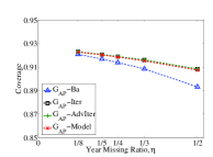
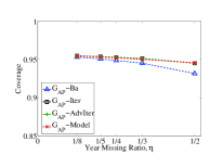
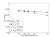
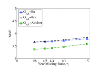
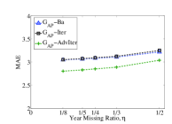
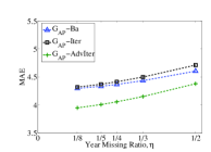
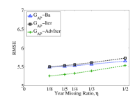
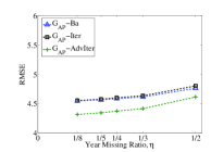
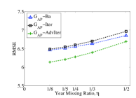
The second set of experiments are conducted on the paper author bipartite network $G_{AP}=(V_{A}\cup V_{P},E_{AP})$. The coverage, MAE and RMSE results of algorithms $G_{AP}$-Ba (the basic scheme), $G_{AP}$-Iter (Simple iteration of the basic scheme) and $G_{AP}$-AdvIter (Iteration with considering Consistent-Coauthor-Pair information) are plotted in Figure 5. Our observations are:

(a) Coverage-Libra

(b) Coverage-DBLP

(c) Coverage-APS

(d) MAE-Libra

(e) MAE-DBLP

(f) MAE-APS

(g) RMSE-Libra

(h) RMSE-DBLP

(i) RMSE-ASP

Figure 5: The coverage, MAE and RMSE of algorithms $G_{AP}$-Ba, $G_{AP}$-Iter and $G_{AP}$-AdvIter in paper author bipartite network $G_{AP}$ of the three data sets

1. In Fig. 5(a)-5(c), the curve of $G_{AP}$-Iter overlaps with that of $G_{AP}$-AdvIter and has better coverage than $G_{AP}$-Ba. As is discussed before (Section 2), $G_{AP}$-Iter and $G_{AP}$-AdvIter utilize the estimation results in the previous rounds for the later iterations (information propagation) which leads to the higher coverage results. In addition, the curves of $G_{AP}$-Iter and $G_{AP}$-Iter match quite well with the expected value generated by the analytical model.

2. In Fig. 5(d)-5(i), which concerns estimation accuracy, we find that $G_{AP}$-Iter obtains worse MAE than $G_{AP}$-Ba. This meets our expectation (in Section 2 that the simple iteration scheme of $G_{AP}$-Iter spreads inaccuracy during the information propagation).

3. It shows that $G_{AP}$-AdvIter performs much better than the other two in both coverage and accuracy. For all different $\eta$, $G_{AP}$-AdvIter consistently makes around $10\%$ improvement in MAE measures and $6\%$ in RMSE measures.

4. If we compare the MAE curves of the three data sets in Fig. 5(d)-5(f), the same algorithm generates the best MAE on DBLP-Cit data set, the worst on APS data set and intermediate on Libra data set. This result indirectly reflects the data quality (on paper-author relationship) of the three data sets, summarized in Table 11. As is widely known that, the original DBLP data set (with no citation information) is well managed and hence maintains the most complete and accurate paper-author/ paper-venue relationships Ley (2009). Libra is an object-level data set, the process of the text-to-object transfer has been done before we obtain them. Different to the paper citation links, the APS data set only provides pure text information of paper-author relationships, therefore, the text-to-object task is done by ourselves with some simple text-based matching scheme, which inevitably induces the number of errors in $G_{AP}$. In fact, this involves several difficult and hot research problems in the community, for example the Author-Paper Identification Challenge and the Author Disambiguation Challenge in KDDCup (2013).

   MYE performance in $G_{AP}$
   Coverage	DBLP $\approx$ Libra $\approx$ APS
   MAE/RMSE	DBLP $<$ Libra $<$ APS
   Inferred data quality of paper-author relationship
   Completeness	DBLP $\approx$ Libra $\approx$ APS
   Correctness	DBLP $>$ Libra $>$ APS

   Table 11: Summary on data quality of paper-author relationship of three used datasets inferred from MYE performance in $G_{AP}$.

3.6 Experiment results for the heterogenous network $G$

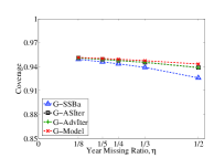
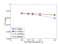
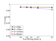
The last set of experiments are conducted on the heterogeneous network $G=(G_{P}\cup G_{AP})$ which consists of both the paper citation network and the paper author bipartite network. The coverage, MAE and RMSE results of algorithms $G$-SSBa (combination of $G_{P}$-SS and $G_{AP}$-Ba), $G$-ASIter (combination of $G_{P}$-AS and $G_{AP}$-Iter) and $G$-AdvIter (combination of $G_{P}$-AA and $G_{AP}$-AdvIter) are plotted in Figure 6.

(a) Coverage-Libra

(b) Coverage-DBLP

(c) Coverage-APS

(d) MAE-Libra

(e) MAE-DBLP

(f) MAE-APS

(g) RMSE-Libra

(h) RMSE-DBLP

(i) RMSE-APS

Figure 6: The Coverage, MAE and RMSE of algorithms $G$-SSBa, $G$-ASIter and $G$-AdvIter in the heterogenous network $G$ of the three data sets.

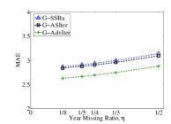
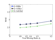
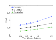
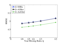
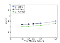
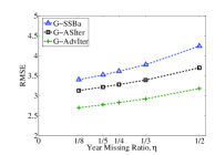
We make three observations according to the results shown in Fig. 6:

1. All the curves have similar shapes as those in Fig.3 and Fig.5, but the results in Fig.6 have the highest coverage and smallest MAE and RMSE. This shows the advantage of the heterogeneous information (both paper citation and paper author relationship) and the proper combination of the MYE algorithms in $G_{P}$ and $G_{AP}$.

2. In Fig. 6(a)-6(c), there appears certain deviations (although milder than those in Fig. 3(a)-3(c)) from the coverage curves of $G$-ASIter and $G$-AdvIter to that generated by the analytical model. This is again due to the overestimation of the expected number of covered papers by the citation network information, since $G$-ASIter and $G$-AdvIter are the combinations from $G_{P}$-AS and $G_{P}$-AA respectively.

3. The $G$-AdvIter outperforms the other two for both coverage and accuracy (with around $8\%$ improvement in MAE and $5\%$ in RMSE for different $\eta$).

4 Related Works

In network analysis, early studies focused on the structural characteristics of missing data, e.g., Kossinets (2006). Borgatti et al (2006) studied the impact of the measurement errors on random Erdős-Rényi networks. A more recent work by Wang et al (2012) reclassifies measurement errors, separating missing data and false data, then analyzes their efforts on different topology properties of an online social network and a publication citation network. However, only few works study techniques to correct measurement errors.

Variants of the well-known PageRank Brin and Page (1998) and HITS Kleinberg (1999) algorithms are often used in social network analysis. Nachenberg et al (2010) use an iterative Belief Propagation Algorithm to identify malware from a large scale of files and machines. Zhu et al (2005) study the propagation of two or more competing labels on a graph, using semi-supervised learning methods.

Temporal information is frequently used in topics of an academic network, e.g. Chiu and Fu (2010); Fu et al (2014). In the research of Academic Rankings, Stringer et al (2008) find nearly all journals will reach a steady-state of citation distribution within a journal-specific time scale, thus they proposed a model for the rank of paper impacts using citation counts. To solve the tricky problem of name disambiguation in a digital library, Tang et al (2012) utilized the multi-hop co-author relationship and its special property of time-dependence. Wang et al (2010) proposed a time-constrained probabilistic factor graph model to mining the highly time-dependent advisor-advisee relationship on the collaboration network.

The topic of evolution of communities also attracts much attention. Blei and Lafferty (2006) have used state space models on the natural parameters of the multinomial distributions to represent the dynamic evolution of topics. Iwata et al (2010) developed the continuous time dynamic model to mine the latent topics through a sequential collection of documents.  Gupta et al (2011) proposed an algorithm that integrates clustering and evolution diagnosis of heterogeneous bibliographic information networks. Lin et al (2011)track the evolution of an arbitrary topic and reveal the latent diffusion paths of that topic in a social community. Li et al (2012) addressed the community detection problem by integrating dynamics and communities into the topic modeling algorithms, and experimented on the Scholarly publications data set ArnetMiner Tang et al (2008), and recently to generalize the preferential attachment model with considering the aging factor Wu et al (2014).

Recently, data cleaning on academic social networks receive much attention. In KDD Cup 2013, the two challenges are the Author-Paper Identification Challenge or the Author Disambiguation Challenge. For both challenges, the publishing year information of each paper is important background knowledge and affect the design of the algorithms. However, the given data set KDDCup (2013) has a high Missing Year Ratio, $\eta=\frac{155784}{2257249}\approx 6.90\%$. This is one of the practical examples and usages that imply the importance of the MYE problems and provide good motivation for this work.

5 Conclusions

In this paper, we are dealing with the papers’ missing publication year recovery problem in the Academic Social Network (ASN). We have considered using three possible networks for estimating missing years: the paper citation network, the paper author bipartite network and the heterogenous network (the combination of the previous two). In each network, we first propose a simple algorithm which is considered as a benchmark. Next another algorithm involving information propagation mechanism is proposed. The propagation mechanism helps to increase the estimation coverage ratio. Finally, an advanced propagation based algorithm is proposed, and in each of the three networks the advanced algorithm outperforms other algorithms and achieves at least an $8\%$ improvement on MAE and $5\%$ on RMSE. In addition, the coverage achieved by the advanced algorithms well matches the results derived by the analytical model.

References

-
APS (2013)
APS (2013) American physical society,
https://publish.aps.org/datasets/ - Blei and Lafferty (2006) Blei D, Lafferty J (2006) Dynamic topic models. In: Proceedings of the 23rd international conference on Machine learning, ACM, pp 113–120
- Borgatti et al (2006) Borgatti S, Carley K, Krackhardt D (2006) On the robustness of centrality measures under conditions of imperfect data. Social Networks 28(2):124–136
- Brin and Page (1998) Brin S, Page L (1998) The anatomy of a large-scale hypertextual web search engine. Computer networks and ISDN systems 30(1):107–117
- Chiu and Fu (2010) Chiu DM, Fu TZ (2010) Publish or perish in the internet age: a study of publication statistics in computer networking research. ACM SIGCOMM Computer Communication Review 40(1):34–43
- Easley and Kleinberg (2010) Easley D, Kleinberg J (2010) Networks, crowds, and markets, vol 8. Cambridge Univ Press
- Fu et al (2014) Fu TZJ, Song Q, Chiu DM (2014) The academic social network. to appear in Scientometrics
- Gupta et al (2011) Gupta M, Aggarwal C, Han J, Sun Y (2011) Evolutionary clustering and analysis of bibliographic networks. In: Advances in Social Networks Analysis and Mining (ASONAM), 2011 International Conference on, IEEE, pp 63–70
- Iwata et al (2010) Iwata T, Yamada T, Sakurai Y, Ueda N (2010) Online multiscale dynamic topic models. In: Proceedings of the 16th ACM SIGKDD international conference on Knowledge discovery and data mining, ACM, pp 663–672
KDDCup (2013)
https://www.kaggle.com/c/kdd-cup-2013-author-paper-identification-challenge/ - Kleinberg (1999) Kleinberg J (1999) Authoritative sources in a hyperlinked environment. Journal of the ACM (JACM) 46(5):604–632
- Kohavi (1995) Kohavi R (1995) A study of cross-validation and bootstrap for accuracy estimation and model selection. In: International joint Conference on artificial intelligence, Lawrence Erlbaum Associates Ltd, vol 14, pp 1137–1145
- Kossinets (2006) Kossinets G (2006) Effects of missing data in social networks. Social networks 28(3):247–268
- Ley (2009) Ley M (2009) Dblp: some lessons learned. Proceedings of the VLDB Endowment 2(2):1493–1500
- Li et al (2012) Li D, Ding Y, Shuai X, Bollen J, Tang J, Chen S, Zhu J, Rocha G (2012) Adding community and dynamic to topic models. Journal of Informetrics 6(2):237–253
Libra (2013)
Libra (2013) Microsoft academic search,
http://academic.research.microsoft.com/ - Lin et al (2011) Lin C, Mei Q, Han J, Jiang Y, Danilevsky M (2011) The joint inference of topic diffusion and evolution in social communities. In: Data Mining (ICDM), 2011 IEEE 11th International Conference on, IEEE, pp 378–387
- Mosteller and Tukey (1968) Mosteller F, Tukey JW (1968) Data analysis, including statistics. In Handbook of Social Psychology
- Nachenberg et al (2010) Nachenberg C, Wilhelm J, Wright A, Faloutsos C (2010) Polonium: Tera-scale graph mining for malware detection
- Stringer et al (2008) Stringer M, Sales-Pardo M, Amaral L (2008) Effectiveness of journal ranking schemes as a tool for locating information. PLoS One 3(2):e1683
- Tang et al (2007) Tang J, Zhang D, Yao L (2007) Social network extraction of academic researchers. In: ICDM’07, pp 292–301
- Tang et al (2008) Tang J, Zhang J, Yao L, Li J, Zhang L, Su Z (2008) Arnetminer: Extraction and mining of academic social networks. In: KDD’08, pp 990–998
- Tang et al (2012) Tang J, Fong A, Wang B, Zhang J (2012) A unified probabilistic framework for name disambiguation in digital library. Knowledge and Data Engineering, IEEE Transactions on 24(6):975–987
- Wang et al (2010) Wang C, Han J, Jia Y, Tang J, Zhang D, Yu Y, Guo J (2010) Mining advisor-advisee relationships from research publication networks. In: Proceedings of the 16th ACM SIGKDD international conference on Knowledge discovery and data mining, ACM, pp 203–212
- Wang et al (2012) Wang D, Shi X, McFarland D, Leskovec J (2012) Measurement error in network data: A re-classification. Social Networks
- Wu et al (2014) Wu Y, Fu TZJ, Chiu DM (2014) Generalized preferential attachment considering aging. Journal of Informetrics 6(3):650–658
- Zhu et al (2005) Zhu X, Lafferty J, Rosenfeld R (2005) Semi-supervised learning with graphs. PhD thesis, Carnegie Mellon University, Language Technologies Institute, School of Computer Science