Warm Dark Matter as a solution to the small scale crisis: new constraints from high redshift Lyman- forest data
Abstract
We present updated constraints on the free-streaming of warm dark matter (WDM) particles derived from an analysis of the Lyman- flux power spectrum measured from high-resolution spectra of 25 quasars obtained with the Keck High Resolution Echelle Spectrometer (HIRES) and the Magellan Inamori Kyocera Echelle (MIKE) spectrograph. We utilize a new suite of high-resolution hydrodynamical simulations that explore WDM masses of 1, 2 and 4 keV (assuming the WDM consists of thermal relics), along with different physically motivated thermal histories. We carefully address different sources of systematic error that may affect our final results and perform an analysis of the Lyman- flux power with conservative error estimates. By using a method that samples the multi-dimensional astrophysical and cosmological parameter space, we obtain a lower limit keV () for warm dark matter particles in the form of early decoupled thermal relics. Adding the Sloan Digital Sky Survey (SDSS) Lyman- flux power spectrum does not improve this limit. Thermal relics of masses 1 keV, 2 keV and 2.5 keV are disfavoured by the data at about the , and C.L., respectively. Our analysis disfavours WDM models where there is a suppression in the linear matter power spectrum at (non-linear) scales corresponding to Mpc which deviates more than 10% from a CDM model. Given this limit, the corresponding “free-streaming mass” below which the mass function may be suppressed is M⊙. There is thus very little room for a contribution of the free-streaming of WDM to the solution of what has been termed the small scale crisis of cold dark matter.
pacs:
98.80.Cqpacs:
98.80.Cq,98.62.Ra,95.35.+dI Introduction
The CDM paradigm, in many respects, has proven to been an immensely successful cosmological model. CDM is based on a cosmological constant plus “cold” dark matter, i.e. dark matter particles whose streaming velocities are negligible for most astrophysical considerations. On large scales, the Planck mission has just delivered another ringing endorsement of this model with its first-year cosmology results planck . On scales below a few (comoving) Mpc, however, the matter power spectrum is still difficult to probe, and it has been repeatedly suggested that dark matter is perhaps “warm”, with a free-streaming length that affects the properties of low-mass (dwarf) galaxies. Warm dark matter (WDM) could alleviate the apparent difficulties of CDM models in reproducing some observations related to the matter power spectrum on scales of a few Mpc and below. The most notable possible tensions under CDM are: the excess of the number of galactic satellites, the cuspiness and high (phase space) density of galactic cores, the luminosities of the Milky Way’s satellites and the properties of galaxies filling voids (e.g. bode ; boylan ; ferrero ; weinberg ).
The main effect of the larger velocities of WDM particles, and the resulting significant free-streaming length, would be to suppress structures on Mpc scales and below. The last few years have seen a re-intensified discussion of this possibility, particularly in light of improvements in numerical models and observations of the mass and internal structure of Local Group satellites libeskind . It has been suggested that a free-streaming length corresponding to that of a thermal relic WDM particle with a mass of 1-2 keV (and in some cases as low as 0.5 keV) provides better agreement between the most recent data and numerical simulations devega ; lovell . The difficulties associated with the cold dark matter paradigm, however, arise on scales where the matter spectrum is highly non-linear at , and where very uncertain baryonic physics is known to play an important role astrophy ; wdm_nonlin ; garrison .
The Lyman- absorption produced by intergalactic neutral hydrogen in the spectra of distant quasars (QSOs)–the so called “Lyman- forest”–provides a powerful alternative tool for constraining dark matter properties, particularly the free-streaming of dark matter particles on the scales in question. The Lyman- forest probes the matter power spectrum in the mildly non-linear regime over a large range of redshifts ( in ground-based data) down to the small scales of interest ( Mpc) croftetal ; Seljak:2006bg . On large scales the SDSS-III BOSS collaboration has recently measured the Baryonic Acoustic Oscillations (BAOs) scale in the 3D correlation function of the Lyman- forest in 50,000 QSOs at BAOs . These findings further emphasize the value of the Lyman- forest as a tracer of cosmological large-scale structure. Constraints on the matter power spectrum from Lyman- forest data on small scales are only limited by the thermal cut-off in the flux power spectrum introduced by pressure and thermal motions of baryons in the photo-ionized intergalactic medium (IGM). The IGM has a characteristic temperature of . While not trivial, modeling the relevant physics with numerical simulations is reasonably straightforward; the power spectrum at the relevant redshifts () and scales is only mildly non-linear and stellar feedback effects are much less important than at lower redshifts vh06 ; feedback .
The basic property of WDM, which impacts on both large scale structure formation and the internal structure of dark matter haloes and the galaxies they are hosting, is the significant “thermal” velocities of the WDM particles (see bode ). The resulting “free-streaming” eliminates density fluctuations on scales below a characteristic comoving wavenumber:
| (1) |
and leads to a very distinctive cut-off in the matter power spectrum at a corresponding scale. For example, the wavenumber at which the linear WDM suppression reaches 50% in terms of matter power, , w.r.t. the CDM case can be approximated as:
| (2) |
where this equation uses the numerical results of Ref. Viel:2005qj . For standard thermal relics, the shape of the cut-off is therefore well characterized in the linear regime and there is an unambiguous relation between the mass of the thermal relic WDM particle and a well-defined free-streaming length (e.g. Viel:2005qj ). Note that we will also quote a free-streaming mass, which is the mass at the mean density enclosed in a half-wavelength mode corresponding to .
For the sake of simplicity, the analysis here is presented in terms of the mass of a thermal relic dark matter particle, for which there is a one-to-one correspondence between the free-streaming length and the particle mass. We should point out, however, that in recent years sterile neutrinos and other non-thermal particles have become popular WDM candidates. Some of these models are actually more similar to mixed dark matter models with cold and warm dark matter components. The shape of the free-streaming “cut-off” can then be quite different from that of a thermal relic, and may instead correspond to a downward step in the power spectrum rather than a cut-off (see sterileboya ; lovell ). There is also no universal relation between free-streaming length and mass of the WDM particles in these models, and the normalization and functional form of this relation varies greatly between different non-thermal WDM candidates. Unfortunately, this has led to considerable confusion in the literature when WDM models, characterized by their model-dependent WDM particle masses, are compared between each other and/or thermal relic models and in particular with Lyman- forest data. For example Ref. lovell quote a sterile neutrino mass of 2keV for their thermal relic WDM model which corresponds, however, to a thermal relic mass of 1.4 keV. For convenience and ease of comparison with the literature, in this work we therefore consider only matter power spectra with cut-off shapes expected for thermal relic WDM particles and quote the unambiguous thermal relic masses (and corresponding cut-off scale) to characterize our WDM models.
The Lyman- forest, due to its spectral nature, probes the matter power spectrum in velocity space. With increasing redshift the ratio of a given (comoving) free-streaming length in velocity space to the thermal cut-off length scale at a given temperature increases as . There is furthermore strong observational evidence that the temperature of the IGM decreases toward higher redshift over the range becker2011a , and therefore a corresponding decrease in the thermal cut-off length scale. Despite observational difficulties, pushing to high redshift allows the models to probe smaller free-streaming lengths and thus to improve the limits on WDM masses. The high-redshift regime has also the advantage of probing structures that are more linear and the WDM cut-off is more prominent at high redshift compared to low redshift wdm_nonlin .
Lyman- forest data to constrain WDM were first used in Ref. Nara where a limit of 750 eV was obtained by using N-body simulations only. In previous work, Ref. Viel:2005qj , we used instead two samples of high-resolution QSO Lyman- forest spectra at to set a lower limit of 550 eV for the mass of a thermal WDM candidate. Following this, Ref. Seljak:2006qw and Ref. Viel:2006kd , using higher-redshift QSO spectra from the Sloan Digital Sky Survey (SDSS) and applying a different analysis method, significantly improved this limit by a factor . As already noted, however, care has to be taken in the correct modeling of the free-streaming properties of “non-thermal” candidate WDM particles of a given model-dependent mass, such as the popular sterile neutrino. In Ref. sterileboya the authors have focused on constraints on a range of such models. Because of a non-zero mixing angle between active and sterile flavour states, X-ray flux observations can also constrain the abundance and decay rate of such WDM particles (e.g. xrayall ). The joint constraints from Lyman- forest data and those from the X-ray fluxes of astrophysical objects now put considerable tension on the parameter space allowed for a sterile neutrino particle with the phase-space distribution proposed by Dodelson & Widrow dw ; CDW , although other, possibly more phsyical scenarios should be explored sterileboya ; kusenko .
In Ref. v08 we presented the most stringent Lyman- forest limits up to that date on the free-streaming of dark matter, m 4 kev (2). That analysis was based on an (at the time) unrivaled sample of high-quality, high resolution QSO absorption spectra extending to . The limit is in obvious conflict with many of the recent suggestions for alleviating the difficulties encountered by numerical models in reproducing the observed properties of Local Group satellite galaxies within the cold dark matter paradigm. These models often assume dark matter to be made up by thermal relic WDM with masses in the range 0.5-2 keV (e.g. lovell ).
Since our study in v08 , the size of our high-quality, high-redshift QSO absorption spectra sample, the quality and size (in particular the dynamic range and resolution) of our numerical simulations and our knowledge of the thermal and ionization state of the IGM at the relevant redshifts have all significantly improved. Motivated by these improvements, and in light of the lively debate of dark matter possibly being warm with masses in the range 0.5-2 keV, we present here a new and much more extensive study of the high-redshift Lyman- forest constraints on the free-streaming properties of dark matter. The new study is based on an improved data set, further refined modeling of the flux power spectrum and a large suite of new numerical hydrodynamical simulations. We also perform a comprehensive investigation of the the systematic uncertainties related to this measurement.
Finally, it is worth highlighting that WDM would have profound implications in many astrophysical and cosmological contexts. In this respect, IGM constraints are highly complementary to other probes based, for example, on the properties of dark matter haloes maccio13 , the number of satellites and their luminosities boylan ; macciofontanot , strong lensing, the velocity function in the local environment zavala , phase-space density constraints shi , the formation of the first stars firststars , the high-redshift quasar luminosity function song , decays of WDM particles in the high redshift universe mapelli , reionization barkana , gamma ray-bursts desouza , galaxy formation aspects menci using N-body/hydrodynamical simulations Wang:2007he ; nonlinear or analytical/semi-analytical methods halomodel ; valageas ; pierpa ; massfunc .
The paper is organized as follows. In Section II we present our new data set. The simulations are described in Section III. The mock quasar sample, which will be important for estimating error amplitude and covariance, is introduced in Section IV. Section V discusses the effect of the most important physical parameters on the flux power spectrum, while most of the remaining nuisance parameters and the impact they have in terms of flux power are discussed in an Appendix. Our main results are reported in Section VI, together with a description of the Monte Carlo sampling of the likelihood space. We summarize our findings and conclude in Section VIII.
II Data
Our analysis is based on high-resolution spectra of 25 quasars with emission redshifts . Compared to our previous analysis in Ref. v08 the number of QSO spectra, at these redshifts, has improved by nearly a factor two. Spectra for fourteen of the objects were taken with the Keck High Resolution Echelle Spectrometer (HIRES) vogt1994 , and the remaining eleven were taken with the Magellan Inamori Kyocera Echelle (MIKE) spectrograph on the Magellan Clay telescope bernstein2002 . Most of the data have been presented elsewhere Becker ; becker2011a ; becker2011b ; calverley2011 . Here we briefly review the relevant features of the spectra, and describe how the flux power spectra were calculated.
The majority of spectra were reduced using a custom set of idl routines based on optimal sky subtraction kelson2003 and optimal extraction horne1986 techniques, while a small subset of the HIRES spectra (PSS 02481802 and BR 12020725) were reduced using the makee software package. The HIRES and MIKE spectra have spectral resolutions of 6.7 and 13.6 km s-1 (FWHM), and the spectra were extracted using 2.1 and 5.0 km s-1 spectral bins, respectively. The one-dimensional relative flux-calibrated spectra were then continuum normalized using spline fits based on power-law extrapolations of the continuum redward of the Lyman- emission line. Median continuum signal-to-noise ratios within the Lyman- forest of each object are typically in the range of per pixel. The continuum estimates are necessarily crude due to the high levels of absorption in the Lyman- forest at these redshifts. We estimate that typical uncertainties in the continuum are of the oder 10-20%, a point we return to in the power spectrum analysis.
To compute the flux power spectra, we first divided the Lyman- forest in each quasar spectrum into two regions of equal redshift length. We then computed the power spectrum of the fractional transmission, , in each region separately, where
| (3) |
Here, is the mean transmitted flux calculated at the mean redshift of each region. We used fixed relations for the mean flux given by , where
| (4) |
The fit to at is from becker2013 , while the evolution at is based on a fit to the mean flux measured from the data presented here. The latter is similar to the trend in presented by fan2006 . We note that our analysis is not sensitive to our choice of using a fixed relation for . In tests where we instead divided each region by the mean flux in that region alone we obtained very similar power spectrum estimates on average. When calculating the flux power spectrum we do not attempt to mask metal lines (see discussion below). We do, however, mask regions of strong telluric absorption (, , , , and Å). The longest-wavelength mask effectively means that we probe up to a maximum redshift of 5.684.
The power spectra for individual regions were averaged over ten logarithmic wavenumber bins in the range with 0.2 dex spacing. The power spectra from all regions were then further averaged according to instrument and the mean redshift in each region. We used median redshifts for a nominal total of eight combined power spectra and 80 data points. In order to be conservative, however, we decided to use a subset of this sample and do not consider the highest redshfit bin for the MIKE data set (which has very large error bars) or the flux power measurements at , which might be affected by continuum fitting uncertainties. The final data set used in the present analysis thus consists of 49 data points.
Preliminary estimates of the error in the power spectra were calculated using a bootstrap approach. It is known, however, that bootstrapping typical underestimates the true errors (e.g. rollinde ). To be conservative, we therefore decided to add an additional 30% uncertainty to our estimates of the errors of the observed flux power spectrum for our standard analysis. We will also quote the tighter limits that would be obtained without this increase of the error estimate. As a further check, we used the set of mock QSO spectra described in Section IV to determine what the expected covariance in the power spectra should be (within the limits of our finite simulation box) at each redshift for a sample of similar size and quality to the one used here. These estimate were used to correct a few error estimates in the real data that appeared to be too small. With these corrections, the final flux power spectra used here have error bars that are larger than .
III Cosmological hydrodynamical simulations
We model the flux power spectrum based on a set of hydrodynamical simulations performed with a modification of the publicly available GADGET-II code. This code implements a simplified star formation criterion Springel:2005mi that turns all gas particles that have an overdensity above 1000 and a temperature below K into star particles. This has been first used and extensively tested in Ref. vhs04 .
The reference model, hereafter referred to as , is a box of length 20 comoving Mpc with gas and cold DM particles (with a gravitational softening length of 1.3 kpc) in a flat CDM universe with cosmological parameters , , and , in agreement both with WMAP-9yr and Planck data wmap7 ; planck . We further explore three different WDM models with masses keV; these models correspond to 50% suppression of power in the linear (redshift independent) matter power spectrum at scales /Mpc, respectively. The initial condition power spectra are generated with CAMBcamb and the suppression and velocity for the WDM particles are implemented using the approach outlined in Ref. Viel:2005qj . In order to assess convergence and evaluate resolution corrections (which are model dependent), we also perform four additional models, one each for the reference and WDM cases, and a single model for the 2 keV simulation only. We also have performed three simulations for CDM, WDM 1 keV and WDM 2 keV in order to check the flux power spectrum convergence at the largest scales of our smaller boxes.
We explore the impact of different thermal histories on the Lyman- forest by modifying the Ultra Violet (UV) background photo-heating rate in the simulations (e.g. Bolton08 ). A power-law temperature-density relation, , arises in the low density IGM () as a natural consequence of the interplay between photo-heating and adiabatic cooling HuiGnedin . We consider a range of values for the temperature at mean density, , and the power-law index of the temperature-density relation, , based on the observational measurements presented recently by Ref. becker2011a . These consist of a set of 3 different indices for the temperature-density relation, , that are kept approximately constant over the redshift range and 3 different temperatures at mean density, K, which evolve with redshift, yielding a total of 9 different thermal histories. The reference thermal history assumes . These 9 thermal histories have been performed for all the 3 WDM models and for the reference CDM case, resulting in a total of 36 simulations.
In addition to these parameters we also consider and vary several other physical parameters for the reference model only, given that these are poorly constrained by the data. These are the redshift of reionization (i.e. the redshift at which the optically thin UV background is switched on in the simulations) which is chosen to be for the reference case and for two additional models; the Hubble constant, with two extra simulations with ; the scalar spectral index, with ; the matter content, with and the r.m.s. amplitude of the matter power spectrum, with . We note here that varying the redshift of reionization in particular enables us to assess the impact of different integrated thermal histories (i.e. the effect of Jeans smoothing, see rorai for a recent discussion) on our analysis. The effect of different integrated thermal histories on Lyman- forest constraints was also considered in Ref. Viel09 using this parameterisation. Overall, a total of 54 hydrodynamical simulations have been performed. Approximately 4000 core hours were required for each (20,512) run to reach , with the higher resolution simulations requiring around 5 times longer.
During the simulation runs, we extract the non-linear matter power spectra in order to compare with wdm_nonlin . For the reference case only, we additioanlly extract the position of the haloes with a friends-of-friends halo finding algorithm for our model of the impact of spatial fluctuations in the UV background on the flux power (see the Appendix for further details).

IV The mock QSO sample
The simulated Lyman- forest spectra are extracted along 5000 random line-of-sights (LOSs) after interpolation of the relevant physical quantities along the LOSs using the SPH formalism. Box-size effects on the flux power are estimated with simulations. Note, however, that the necesary box size correction is below the percent level at the largest scales used. Resolution corrections are, however, important. The flux power spectra are corrected for resolution effects using the simulations (see the Appendix for further details).
The mean flux is varied a posteriori, after having extracted the spectra, by reproducing times the observed (see Appendix). At the end of the procedure the four-dimensional parameter space in is explored fully by means of quadrilinear interpolation performed over the set of 36 hydrodynamical simulations and 108 ( mean flux values) flux models.
In order to get a better understanding of the expected (co)variance properties of the observed data we generate samples of mock QSO absorption spectra which resemble the observational data as closely as possible. The procedure used to create the mock spectra can be summarized as follows: we consider the total redshift path in each redshift bin and combine the short simulated spectra ( Mpc in length) to match the total length of an observed QSO spectrum (approximately 40 spectra are used); we allow for an optical depth evolution along the LOS (which is absent since our simulated spectra are from snapshots at fixed redshifts) following the scaling expected from the fluctuating Gunn-Peterson approximation, (see e.g. rauch97 ); for each short simulated spectrum we consider a 20% error on the quasar continuum placement (the continuum is drawn randomly from a Gaussian distribution around the value 1 with a ); we smooth the flux with a Gaussian at a given FWHM corresponding to the spectrograph resolution and rebin the spectra with the observed pixel-size; we add Gaussian-distributed noise on top of the flux, matching the signal-to-noise of the observational data. We demonstrate in the Appendix that the (instrumental) effects of noise and finite resolution, which are scale and redshift dependent, are below 20% (6%) at the smallest scales for MIKE (HIRES).
The (co)variance properties of this mock sample are in reasonable agreement with those of our observed sample, both as a function of redshift and wavenumber. There are only 5 data points that appear to have error bars that are smaller than those obtained from the mock sample: 4 data points from the MIKE sample ((s/km) at , (s/km) at , (s/km) at ) and one data point from the HIRES sample ( at ). As the observed sample is still small and it is thus expected that the bootstrap errors estimated from the data could be unrealistically small, for these data points we increase the error bars to match those obtained from a mock sample of 30 QSOs in the same redshift bin. These mock data points, with the extra 30% error added, otherwise agree well with those of the observational data, giving us confidence that this is reasonable.
Finally, we note that the hydrodynamical simulations used to construct our mock Lyman- forest spectra do not incorporate chemical elements other than hydrogen and helium. We have therefore estimated how unidentified, lower redshift metal lines in the Lyman- forest may bias our result, and in particular how these narrow absorption lines may alter the flux power spectrum at small scales. Furthermore, the simulations also assume a spatially uniform UV background. We therefore also estimate the impact of spatial fluctuations in the UV background on the Lyman- forest at –. We follow a modified version of the approach described in Ref. BoltonViel11 for exploring fluctuations in the Heionising background at lower redshift, to which we refer the reader for further details. These two systematics effects will also be discussed more extensively in the Appendix.
V The flux power spectrum
V.1 The WDM and thermal cut-offs
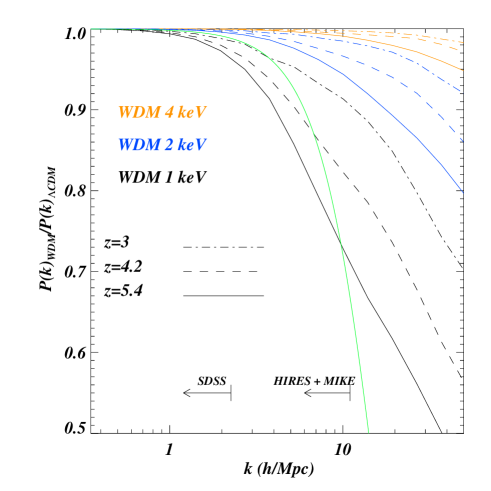
In this Section we demonstrate the distinctively different effects that the thermal (i.e. due to the temperature of the photo-ionized IGM) and WDM cut-off have on the flux power spectrum. We will also check for possible effects due to the limited numerical resolution of our simulations. Firstly, however, it is instructive to consider Fig. 1, where we show the ratio of the non-linear matter power spectra in the WDM and CDM simulations. The results are shown at three different redshifts, . The redshift range – brackets that of the high-resolution data set used in this work. We additionally present the matter power spectrum at to show the evolution of the non-linear power at lower redshift. The three WDM models are reported as orange, blue and black curves for masses of 4,2 and 1 keV, respectively, while the green curve shows the linear suppression for the 2 keV case taken from Ref. Viel:2005qj . The power spectra are already clearly somewhat non-linear at high redshift; the blue and green curves start to differ significantly at small scales at Mpc. In the bottom part of the panel we show the approximate wavenumber ranges that are probed by SDSS and the HIRES+MIKE data set used in our analysis. Note that the non-linear matter suppression is in good agreement with the fitting formula presented in Ref. wdm_nonlin .
In Figure 2 we qualitatively compare a set of noiseless Lyman- forest spectra extracted from the CDM, WDM 1 keV and WDM 2 keV models, represented by the green, black and blue curves respectively. It is clear that the amount of small-scale substructure in the transmitted flux in the CDM is more prominent with respect to the WDM cases. In the rest of this Section we will quantify these differences in terms of the 1D flux power spectrum.
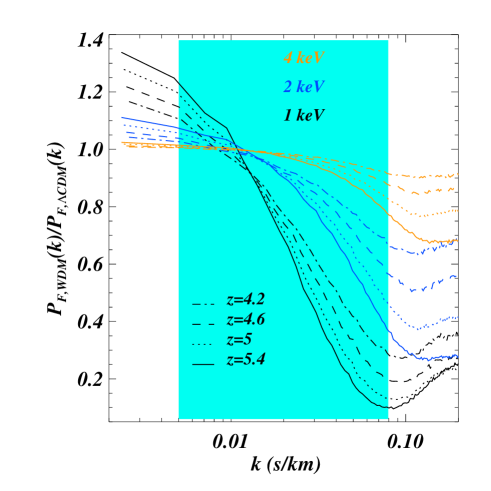
We now turn to Figure 3, which shows the ratio between the 1D flux power of the WDM and CDM models for the four different redshift bins used in the present analysis (note that we compute the power spectrum of the quantity , and we refer to this as the flux power). The suppression of the flux power is larger than that seen in the matter power spectrum. This is due to the fact that the 1D matter power spectrum is an integral of the 3D power spectrum and therefore very sensitive to the small scale cut-off. As expected, the largest differences exist between the 1 keV (black curves) and the CDM model. Note that the flux power also changes at large scales; the requirement of reproducing the same observed mean flux value (given by Eq. 4) results in an increase of the power at those scales (the power spectrum of the WDM flux , not , does show suppression over all scales when compared to CDM). Furthermore, we also note that there is a substantial redshift evolution of the flux power between and .
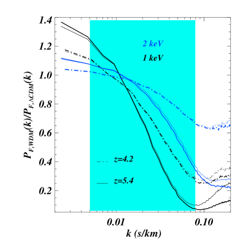
Numerical convergence for WDM simulations can be particularly difficult to achieve (see Ref. Wang:2007he ). In Figure 4 we demonstrate that at the resolution and WDM masses considered in this work, this should, however, not be an issue. Figure 4 compares the flux power extracted from the and 1 and 2 keV simulations to the corresponding CDM simulations at the same resolution. The agreement between the different resolution simulations is very good, typically at the percent level. The differences are largest for the 1 keV case at the smallest scales probed by our data in the current analysis, where they reach the 10% level. The simulated flux power spectra for both CDM and WDM models have therefore been corrected for resolution effects by multiplying the raw power spectra by the ratio of the results from the and simulations. In general, we find the requirements for reaching numerical convergence in terms of flux power are more demanding for absolute values of the flux power rather than ratios of different models w.r.t. the CDM case. This will be discussed further in the Appendix.
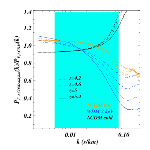
In Figures 5 and 6 we explore the effects of the two thermal parameters, and , on the flux power spectrum. As discussed earlier, the relation is usually parameterized as a power-law, . In both of these figures we also plot the WDM 2keV model in order to emphasize the very distinct differences between the thermal and WDM cut-offs, both in the dependence on wavenumber and redshift. A hotter (colder) value produces a suppression (enhancement) in the flux power spectrum with a redshift dependent cut-off. The WDM cut-off is instead more pronounced and steeper than the cut-off induced by a hotter IGM. The dependence of the thermal cut-off on the slope of the temperature-density is Fig. 6 is also very different from the wavenumber and redshift dependence of the WDM cut-offs, and is much flatter over the wavenumber range considered here.
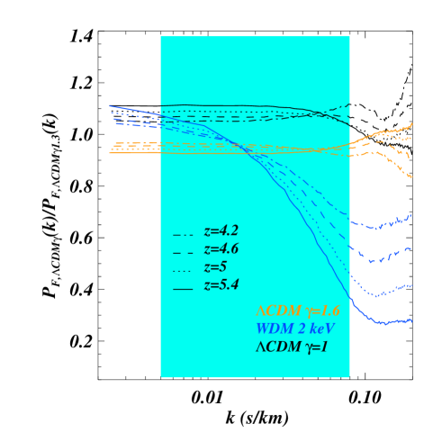
The effects due to to changing the mean flux level are discussed in detail in the Appendix (Fig. 17). We conservatively assume a range of for the observed effective optical depth. We further note that the dependence of changing the mean flux level on wavenumber is even flatter than that obtained for variations of , but shows a weak scale dependence in the highest redshift bin.
V.2 Systematic uncertainties
In this Section we now briefly discuss the following systematic effects: instrumental resolution; noise; spatial fluctations in the UV background and metal line contamination. In the Appendix there is a more detailed description of these nuisance effects and how they are modeled. We only summarize the main quantitative results here. Instrumental resolution, which is different for the two sub-data sets, suppresses the flux power spectrum by at most 20% and 5% for MIKE and HIRES, respectively, at the smallest scales probed, with a negligible redshift dependence. The signal-to-noise ratio impacts at about the 2-3% level at the smallest scales for while it is at the 7% level for the highest redshift bin.
The UV background fluctuations have been implemented with a deliberately extreme model based on ionizing emission from quasars only. The impact of this extreme model of UV fluctuations on the flux power spectrum is quite scale dependent, and rises considerably at large scales (see also UV ). At the scales of interest here the effect on the flux power spectrum is below the 10% level (see Figure 15). This should be considered as a generous upper limit. The metal contamination has a much smaller effect on the flux power spectrum, below the 1% level for the whole range of scales considered (see Figure 16). Apart from the apparently negligible metal contamination, the other nuisance effects have been fully implemented in our analysis.
In Table I, we summarize the main nuisance parameters and present rough estimates of the relative errors induced in the flux power spectrum. Where possible, effects with a known amplitude such as resolution and noise characteristics are simply incorporated into the mock QSO spectra. The remaining parameters are fully marginalized over in our likelihood analysis.
| syst. eff. | Notes | |
|---|---|---|
| data res. | % | corrected |
| data S/N | % | corrected |
| num. res. | % | corrected |
| metals | % | neglected |
| mean flux | % | marginalized |
| thermal history | % | marginalized |
| UV | % | marginalized |
VI Method and Results
We now turn to our analysis of the data and discuss our results. For all 108 flux models considered in our analysis, we compute the ratio of these models with respect to the reference model. We then bin this ratio at the same wavenumbers as the data. In practice, this means we have a 4D parameter matrix with that summarizes all the results obtained from the hydrodynamical simulations, plus some further parameters for which we have established the effect on the flux power for the reference model only. We parameterize the effect of UV background fluctuations on the flux power with a factor that multiplies the flux power spectrum corrections shown in Fig. 16, constrained to be in the range and applied in addition to the corrections discussed in the previous Section ( means that the power spectrum is corrected exactly by the amount shown in the lower panel of Fig. 16). We decide to neglect the effect of metal contamination since it is, as we discuss further in the Appendix, very small. We then perform second order Taylor interpolations for the following remaining parameters: , as in Refs. Viel:2005ha ; v08 .
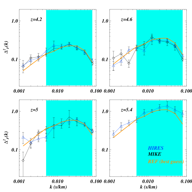
In Figure 7 we compare our best-guess model (the reference simulation), represented by the orange curves, with the observational data. This best-guess model will be the reference point of our likelihood code that will be described below. Note that there is already rough “visual” agreement with the data, albeit with a poor value.

We use a modified version of the code COSMOMC Lewis:2002ah to derive parameter likelihoods from the Lyman- forest data. For the HIRES+MIKE data, we have a set of 15 parameters: 6 cosmological parameters (, , ); 4 parameters describing the thermal state of the IGM, using a power-law parameterization of the temperature-density relation, , with parameters and ; 4 parameters describing the evolution of the effective optical depth with redshift, since a single power-law has been shown to be a poor approximation over this wide redshift range (see Becker ) and one parameter describing the spatial fluctuations in the UV background . We apply strong Gaussian priors to in order to mimic Planck constraints: . We have checked that these priors do not affect any of our constraints on the free-streaming length/WDM mass, but they are helpful in obtaining faster convergence of the Monte-Carlo chains. We vary in the range K and in the range , and thereby heavily penalize the if is outside the physical range . The values of and are not constrained by the data and they are prior dependent: the range chosen are km/s/Mpc and , respectively.
The covariance matrix calculated from our data set is noisy (especially at high redshift), preventing a reliable inversion. We have therefore regularized the observed covariance matrix with the correlation coefficients as estimated from the simulated spectra as in Ref. Lidz:2005gz , with , where and are the covariance matrices of the observed and simulated spectra, respectively.
| parameter | (1) | (2) | best fit |
|---|---|---|---|
| [] | [] | 0.957 | |
| [] | [] | 0.822 | |
| [] | [] | 0.298 | |
| [] | [] | 1.16 | |
| [] | [] | 1.32 | |
| [] | [] | 1.91 | |
| [] | [] | 3.09 | |
| [] | [] | 1.64 | |
| [] | [] | -0.15 | |
| K | [] | [] | 9.2 |
| K | [] | [] | -2.5 |
| [] | [] | 0.18 | |
| [] | [] | 11.2 | |
| keV/ | [] | [] | 0.03 |
Our results are summarized in Table 2. We obtain a upper limit on the parameter 1keV of 0.3,which translates into the following constraints: keV at the C.L. and keV at the C.L., with a best-fit value of keV. For a keV WDM particle the 50% suppression in the 3D linear matter power compared to the CDM case matter power spectrum is at a scale of Mpc, while the suppression at Mpc is about 10%. If we drop the 30% additional error applied to the observed flux power spectrum (see Section II) we get a tighter lower limit of keV (). The gets worse by , but still has a probability of 11% of being this large for the present number of degrees of freedom.
We also took a “frequentist” approach and fixed the values of to 2.5 and 3.3 keV and found the results in terms of the other parameters: in this case the is of course higher than in the CDM model (with , respectively) but nevertheless compatible with the results obtained in our standard analysis. This is similar to the approach used in Ref. cwdm , in which an analysis of mixed cold and warm models was performed in both a Bayesian and in a frequentist approach.
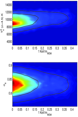
The degeneracies between the parameter 1keV and the other parameters are very weak. In Fig. 8 we show the 2D contour plots for the mean likelihood (in colour) and the marginalized likelihood (black curves) for and versus 1 keV/. In Fig. 9 we report the 1D mean and marginalized likelihoods for 1keV (continuous and dotted curves, respectively).
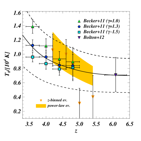
We obtain the following evolution for the temperature-density relation K and . The inferred temperature is decreasing with increasing redshift, while the redshift evolution of is weak. We stress that the IGM thermal state is just one of several nuisance parameter in our likelihood analysis over which we marginalise. We discuss it here in the context of a consistency check rather than as a measurement. With this in mind, in Figure 10 we show the recovered redshift evolution for compared to three input thermal histories used in the simulations and measurements obtained from high resolution Lyman- forest data from Refs. becker2011a ; bolton12 (note that the power-law index of the temperature-density relation, , has not yet been measured directly at ). The shaded orange area brackets the of the temperatures obtained by our standard likelihood analysis after marginalization. The inferred temperature evolution (parameterized as a power law in redshift) is in good agreement with the measurements from Ref. becker2011a . We also tested a model where the IGM temperature is left to vary freely in the four redshift bins, shown by the orange data points with error bars in Figure 10. In the two highest redshift bins this analysis returns temperatures that are rather cold and are disfavored by the data with an unreasonably large temperature jump between and (see Fig. 10). This suggests that in this case we have introduced too many free parameters and are most likely “overfitting” the flux power spectrum. For completeness we mention that with this apparently unphysical temperature evolution our analysis gives a constraint on ( C.L.) which is about 1 keV lower than for our standard analysis and also returns an unreasonably low reduced value. Finally we have also performed a likelihood analysis where the IGM temperature is fixed to be unrealistically cold throughout (3000K, independent of redshift) to allow for a maximum contribution of the free-straming of WDM to the observed cut-off in the flux power. Again just for completeness, for this model the constraint on ( C.L.) is lower by about 0.5 keV compared to our standard analysis.
The recovered effective optical depth values at each redshift bin are usually within 20% of the measured optical depth evolution used as the input into the likelihood calculation. The inferred values for the amplitude and slope of the matter power spectrum and for the matter content do not show biases with respect to the Planck-like priors we used. Overall the for the best fit model is 34 for 37 d.o.f. which has a reasonably high probability of about 60% of being larger than this value.
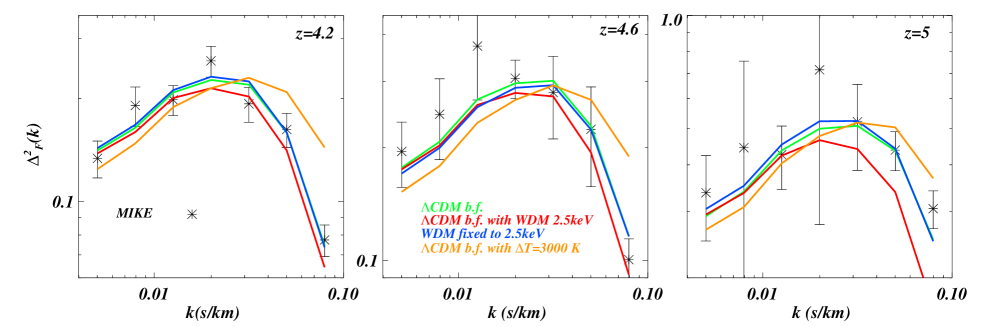
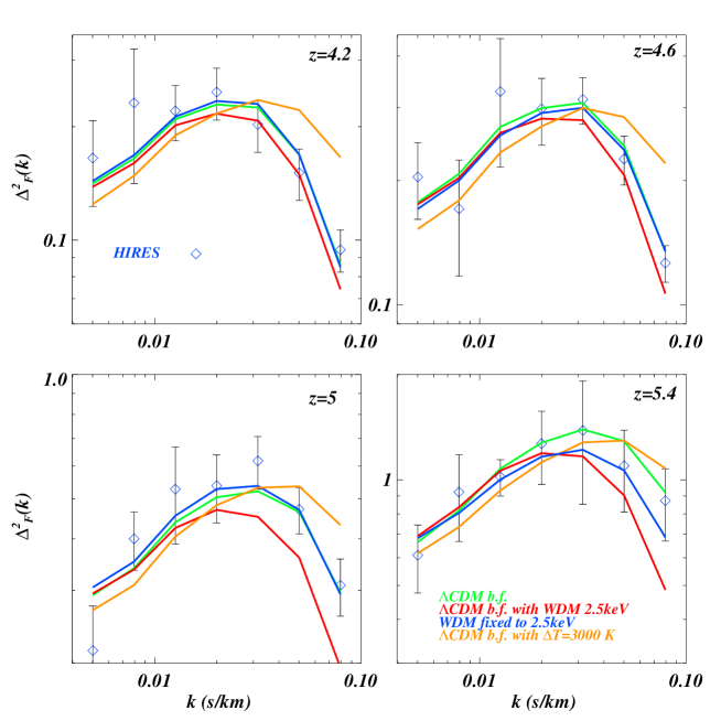
Lastly, in Figures 11 and 12 we show our final best-fit model compared to the data obtained with MIKE and HIRES, respectively. The best fit model is shown as the green curves. We also overplot, for comparison purposes only, three other models that are excluded with very high significance by the present analysis: a model which has a WDM mass of keV (red curves) and a hot model with a temperature value which has been increased by 3000 K with respect to the best fit case (orange curves). When calculating the predicted flux power spectrum for these three models we change only one parameter each time and leave all other parameters fixed at their overall best fit values. In addition, we show the case in which fix keV and allow all other parameters to assume their best-fitting values under this assumption (blue curves).
Compared to our previous findings obtained in Ref. v08 , it is worth stressing the main differences. First of all, from the data side, the sample used here extends to high redshift and double the amount of spectra contributing to the signal at . Secondly, both the simulations and the analysis have been refined by: increasing the number of hydrodynamical simulations and their resolution; improving the method in a way that allows a full sampling of the most relevant parameter space (thermal parameters, WDM cutoff and mean flux) compared to a poorer sampling of the parameter space made in Ref. v08 . When considering only the high-resolution data set, we improve the limits by nearly a factor three from 1.2 keV to 3.3 keV at the C.L., this is due to both the data and the modelling of the flux power.
VII Joint analysis with SDSS data
In this Section we present the joint analysis with the Sloan Digital Sky Survey (SDSS) 1D flux power spectrum data of Ref. McDonald:2004xn where the authors have presented the flux power spectrum of a sample of 3035 QSO absorption in the redshift range drawn from the DR1 and DR2 data releases of SDSS. These data have a spectral resolution of R , and so typical Lyman- absorption features, which have a velocity width of km s-1, are not resolved. The wide redshift range, however, makes this data set very constraining in terms of cosmological parameters. As a final result of their analysis they present an estimate of flux power spectrum at 12 wavenumbers in the range (s/km), equally spaced in for for a total of 132 data points. This measurement is likely to improve soon with the new analysis made by the SDSS-III team of a sample which is about 50 times larger than the one we utilize here palanque .
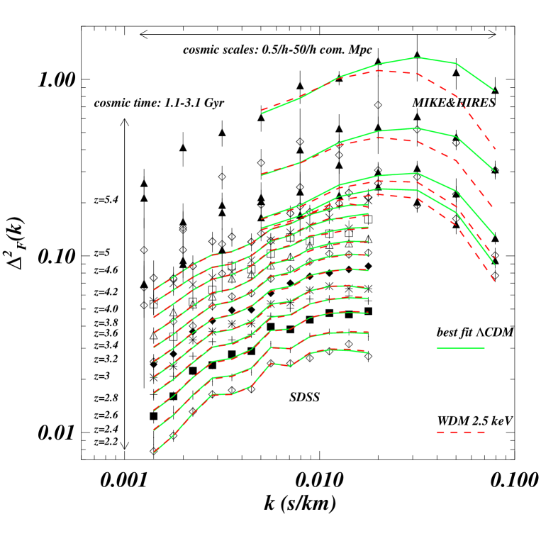
For the joint SDSS+MIKE+HIRES analysis we have used a total of 28 parameters: 15 parameters as used for the HIRES/MIKE spectra (without and the two parameters describing the effective optical depth evolution at ) plus 13 noise-related parameters: 1 parameter which accounts for the contribution of Damped-Lyman- systems and 12 parameters modeling the resolution and the noise properties of the SDSS data set (see McDonald:2004xn ). We do not consider the possible effect of different reionisation scenarios on the SDSS flux power. The covariance matrix of the SDSS flux power is provided by the authors of McDonald:2004eu . The lower limit on is unchanged at 3.3 keV but now with a for the best fit model for a total of 181 data points and 170 degrees of freedom, which has a 23% probability of being this large. Given the fact that the SDSS and MIKE+HIRES data sets do not have redshift overlap there is no significant bias in the other recovered marginalized parameters. Note that for the joint analysis we used the SDSS likelihood based on second order Taylor expansion of the flux power as described in Ref. vh06 and used in Ref. v08 .
Unlike our previous findings obtained in Ref. v08 , where the wide redshift range of SDSS data was helpful in breaking the degeneracies between thermal parameters and WDM cutoff, we notice that in this case the SDSS data do not improve the overall constraints. This means that the constraining power of the new high-resolution data set is higher than the low-resolution SDSS data. The joint analysis gives now a lower limit of 3.3 keV, compared to the previous 4 keV value is thereby slightly less stringent: this is due to the different interplay between the data sets and to the relative role of the degeneracies present between IGM thermal state and WDM cut-off. It is also important to stress that the 30% extra error budget on the high-resolution data impacts on the final results also for the joint analysis making the results less stringent than in Ref. v08 , where this error was not present.
VIII Discussion and Conclusions
| model | (1) | (2) | best fit | /d.o.f. |
|---|---|---|---|---|
| REF. | keV | keV | 33 keV | 34/37 |
| REF. w/o 30% | keV | keV | 100 keV | 48/37 |
| REF. w/o covmat | keV | keV | 14.3 keV | 33.2/37 |
| REF. + SDSS | keV | keV | 42 keV | 183.3/170 |
We have presented a comprehensive analysis of the transmitted Lyman- flux power spectrum extracted from a set of 25 high-resolution QSO spectra taken with the HIRES and MIKE spectrographs. This represents an improved and extended version of the sample originally analysed in v08 . The Lyman- forest is an excellent probe of the matter distribution at intermediate and high redshift in the mildly non-linear regime, from sub-Mpc up to BAO scales. In this work we have focused on constraining any possible suppression of the total matter power spectrum which could be induced by the free-streaming of WDM particles in the form of a thermal relic. Due to the non-linear nature of the the relationship between the observed Lyman- flux and underlying matter density, departures from the standard CDM case are expected over a range of scales that span at least one decade in wavenumber space and can be constrained by the data used in the present analysis. We model this suppression by using a set of high-resolution hydrodynamical simulations and by marginalizing over a large range of physically motivated thermal histories.
The WDM cut-off exhibits a distinctive behavior which we demonstrate is not degenerate with other physical effects due to its different redshift and scale dependence. We consider possible sources of systematic errors including metal line contamination, spatial fluctuations in the UV background intensity and uncertainties in the mean flux level estimation. Galactic feedback either in the form of supernova driven galactic winds or Active Galactic Nuclei (AGN) feedback should not impact the flux power spectra at the high redshift considered in this analysis feedback .
Our final results are obtained by means of a Monte Carlo Markov Chain likelihood analysis around a best-guess reference model. The constraints quoted for have been calculated after marginalization over the other astrophysical and cosmological parameters. Our analysis is conservative in the following sense: we have dropped the estimates of the power spectrum at the largest scales probed by our sample in order not to be sensitive to continuum fitting uncertainties; we add an additional error of about 30% to our error estimates obtained by bootstrapping to account for the expected underestimation of the real error; and we allow for large fluctuations in the UV background fluctuations, which appear to be the most important nuisance factor. Furthermore, we create a mock QSO sample which resembles as closely as possible the real data including noise and resolution and use the covariance matrix of this mock sample as an estimate of the error properties of the real data. Our final result of this analysis is keV at the C.L., where the mass refers to that of a thermal relic. This mass implies that WDM models for which there is a suppression in terms of the 3D linear matter power at scales /Mpc (/Mpc) larger than 10% (50%) when compared to the CDM case, are disfavoured by the present data sets. The corresponding value of the “free-streaming” mass is . A model with a 2.5 keV thermal relic mass is disfavoured by the data at about C.L., a 2 keV mass at about C.L., and a keV model at about C.L. Our final marginalized estimates and best fit values for are summarized in Table III.
Overall, the final results presented are similar to those we have obtained in our previous analysis Ref. v08 [3.3 (4.5) keV vs 4 keV previously if we include (do not include) an additional 30% error to account for a possible underestimate of the statistical error from a boot-strapping analysis). We emphasize, however, that the present analysis is considerably more robust. It uses a larger data set, a much improved analysis based on a broader suite of significantly improved simulations and as well as an extensive analysis of the systematic uncertainties.
Further improvement of the constraints on the free-streaming of dark matter particles from Lyman- forest data could come mainly from an enlarged set of high-quality, high resolution spectra, especially at the highest redshifts where the flux power spectrum is most sensitive to the free-streaming of dark matter. An increase of the dynamical range of the simulations and improved independent constraints on the thermal state and thermal history of the IGM are next on the list as requirements for further corroborating and perhaps pushing the constraints to even larger thermal relic masses. In the future, considerably stronger constraints on WDM may be derived using a baryonic tracer which is colder than the photo-ionized IGM, thus moving the thermal cutoff to smaller scales in the flux power spectrum. Studies of 21 cm absorption/emission by neutral hydrogen gas before reionization, for example, could eventually fulfill this requirement.
However, with a lower limit of M for the mass of dark matter haloes whose abundance could still be significantly affected, the Lyman- forest data appears to leave already very little room for a contribution of the free-streaming of warm dark matter to the solution of what has been termed the small scale crisis of cold dark matter. In particular, recent suggestions for models with relic masses of 0.5-2keV are significantly disfavoured by our analysis. We finally note that our analysis also suggests that it is unlikely that sterile neutrinos could act in that role.
Acknowledgements
A part of the observations were made at the W.M. Keck Observatory which is operated as a scientific partnership between the California Institute of Technology and the University of California; it was made possible by the generous support of the W.M. Keck Foundation. This paper also includes data gathered with the 6.5 meter Magellan Telescopes located at Las Campanas Observatory, Chile. The authors wish to recognize and acknowledge the very significant cultural role and reverence that the summit of Mauna Kea has always had within the indigenous Hawaiian community. We are most fortunate to have the opportunity to conduct observations from this mountain. The hydrodynamical simulations in this work were performed using the COSMOS Supercomputer in Cambridge (UK), which is sponsored by SGI, Intel, HEFCE and the Darwin Supercomputer of the University of Cambridge High Performance Computing Service (http://www.hpc.cam.ac.uk/), provided by Dell Inc. using Strategic Research Infrastructure Funding from the Higher Education Funding Council for England. COSMOS and DARWIN are part of the DIRAC high performance computing facility funded by STFC. MV is supported by the FP7 ERC grant “cosmoIGM” GA-257670, PRIN-MIUR and INFN/PD51 grants. GDB acknowledges support from the Kavli foundation. JSB acknowledges the support of a Royal Society University Research Fellowship. MH acknowledges support by the FP7 ERC Grant Emergence-320596.
*
Appendix A Systematics
A.1 Numerical Convergence
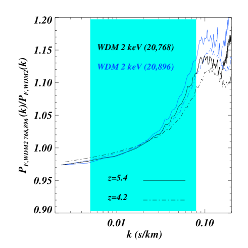
In Figure 14 we compare the 1D flux power spectrum extracted from the WDM 2 keV and models to our reference resolution of . We focus on this WDM mass since it is excluded at high significance by our analysis, yet it is used by the large scale structure community in order to solve apparent problems of CDM at small scales. There is at most a 10-12% correction at the smallest scales probed in our analysis ( s/km) when the flux power spectra from the model are considered, and there is an extra 2% correction when the is considered. After correcting for this, we therefore believe that we have reached 5% agreement in terms of the flux power for the smallest scales considered in this work. This is below the 7.75% (1) statistical error of the data at the same wavenumber.
A.2 Instrumental Effects on the Flux Power
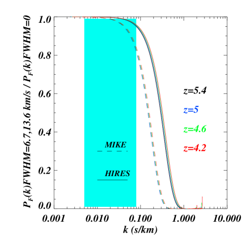
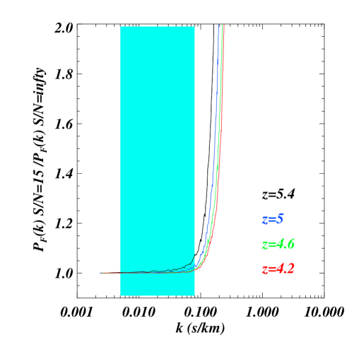
In Figure 15 we show the effect that instrumental resolution and a given signal-to-noise (S/N) ratio has on the Lyman- flux power spectrum in the four different redshift bins of our data sample. These results have been obtained from our mock QSO spectra sample. Note that both of these effects have been incorporated into the Lyman- forest spectra used in our analysis. The S/N ratio results in an increase in the flux power of less than 5% over the range of wavenumbers considered in this work, while instrumental resolution effects are particularly important for the MIKE sample. There is a 20% correction at the smallest scales for the MIKE data (for the HIRES data this value is 5%).
A.3 Systematic Effects on the Flux Power induced by Metals and UV background fluctuations
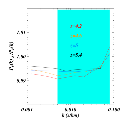
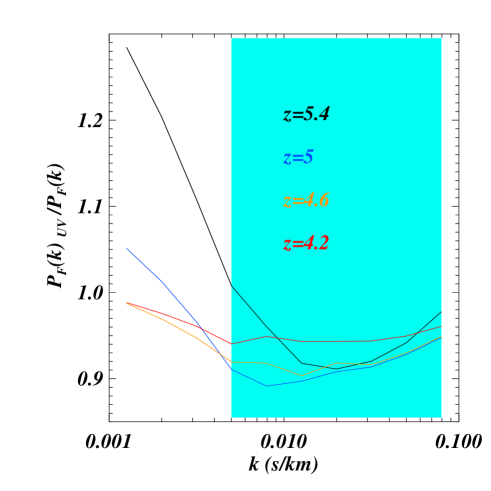
We also consider two important astrophysical nuissance effects in this work: unwanted contamination from metal lines in the Lyman- forest and the effect of spatial fluctuations in the UV background intensity on the observed Lyman- forest transmission.
In the redshift range we consider in this work, –, the most common metal lines in the Lyman- forest will arise from absorbers at lower redshifts. We therefore consider the effect of absorption from three prominent absorption line doublets; C(1548, 1551), Si(1394, 1403) and Mg(2796, 2804), arising over the redshift intervals –, – and –, respectively.
We add these metal lines to Lyman- forest spectra drawn from our reference CDM hydrodynamical model using the following prodcedure. We firstly integrate fits to the column density distribution functions (CDDFs) presented by Scannapieco06 from a set of 19 high resolution VLT/UVES quasar spectra at – over the column density range -, for all three species. We then multiply the results by the redshift path length of our Lyman- forest data set to provide an estimate of the number of metal line absorbers in the Lyman- forest. Note that this approach will likely overestimate the number of Cand Siabsorbers due to the somewhat lower redshift coverage of the Scannapieco06 dataset relative to this work. Our metal contamination estimates are therefore likely to be conservative in this regard. Next, we Monte Carlo sample column densities and line widths for the appropriate number of lines from the Scannapieco06 CDDF fits and the Doppler parameter distribution given by Ref. HuiRutledge99 , with a chosen value for all three species. Finally, we randomly insert these absorption features into the sight-lines in our mock Lyman- forest data set.
In order to estimate the impact of spatial fluctuations in the UV background on the Lyman- forest at – we use a modified version of the approach described in BoltonViel11 , which was used to examine fluctuations in the Heionising background at lower redshift. We refer the reader to Ref. BoltonViel11 for further details. The key difference in this work is that we compute the spatially varying Hphoto-ionisation rate along our simulated sight-lines. We achieve this by computing the specific intensity of the ionising background between – (replacing equation 3 in BoltonViel11 ) by solving:
| (5) |
where is the frequency of the Hionisation edge, is the mean free path for ionising photons presented by Songaila10 and is the power-law slope of the HCDDF Kim02 . The summation in eq. 5 is over all quasars with luminosities, , drawn from the Hopkins07 B-band quasar luminosity function. In order to be conservative, in this work we adopt an extreme model which maximises the effect of the UV fluctuations on the Lyman- forest by assuming all ionising photons in the IGM at – are produced by quasars with . We therefore ignore the significant contribution to the UV background from the more numerous, fainter star-forming galaxies at these redshifts, which effectively smooth out the large-scale fluctuations produced by the rarer quasars. The spatially fluctuating photo-ionisation rates are then obtained by integrating the specific intensity with respect to frequency, weighted by the photo-ionisation cross-section.
In Figure 16 we show the effect that UV fluctuations and metal contamination have on the flux power spectrum. In the wavenumber range considered here, the UV background fluctuations have an effect at around the 10% level at the largest scales, dropping to 5% at smallest scales considered in this work. The effect is larger at high redshift (z=5,5.4) than in the two other redshift bins. Metal contamination affects the flux power very little (at the level) and is at a level below the statistical error bars of our data.
A.4 Mean flux level uncertainties
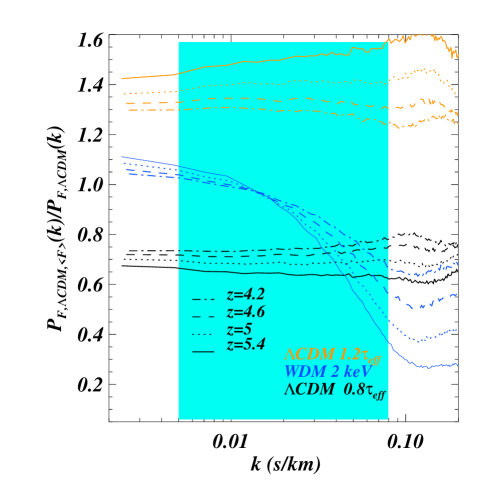
The mean flux level , or alternatively the effective optical depth , is a key ingredient in our flux modeling procedure and a quantity that needs to be marginalized over in the Monte Carlo Markov Chain likelihood estmation. In Figure 17 we demonstrate the effect that a different mean flux level has on the flux power spectrum. We choose two different mean flux levels with 20% higher and lower than the reference value (which corresponds to the observed mean flux). A higher (lower) value for will result in more (less) power relative to the reference value. The trends are similar to those found for the evolution of , i.e. rather flat in wavenumber space, with some weak scale-dependence which is only present in the highest and lowest redshift bins. Our final results are not sensitive to the actual choice of the effective optical depth values, since these are marginalized over in the likelihood estimation.
References
- (1) Planck 2013 results. XVI. Ade, P. A. R., eprint arXiv:1303.5076
- (2) P. Bode, J. P. Ostriker and N. Turok, Astrophys. J. 556, 93 (2001); B. Moore, T. Quinn, F. Governato, J. Stadel and G. Lake, Mon. Not. Roy. Astron. Soc. 310, 1147 (1999); V. Avila-Reese, P. Colin, O. Valenzuela, E. D’Onghia and C. Firmani, Astrophys. J. 559, 516 (2001); M. Miranda, Macció A.V, Mon. Not. Roy. Astron. Soc. 366, 1529 (2006).
- (3) Boylan-Kolchin, Michael; Bullock, James S.; Kaplinghat, Manoj, Mon. Not. Roy. Astron. Soc. 422, 1203 (2012); Peñarrubia, Jorge; Pontzen, Andrew; Walker, Matthew G.; Koposov, Sergey E., ApJ, 759, 42, (2012).
- (4) Ferrero, Ismael; Abadi, Mario G.; Navarro, Julio F.; Sales, Laura V.; Gurovich, Sebastiュマ, Mon. Not. Roy. Astron. Soc. 452, 281 (2012).
- (5) Weinberg, David H.; Bullock, James S.; Governato, Fabio; Kuzio de Naray, Rachel; Peter, Annika H. G., eprint arXiv:1306.0913 (2013).
- (6) Libeskind, Noam I.; Di Cintio, Arianna; Knebe, Alexander; Yepes, Gustavo; Gottloeber, Stefan; Steinmetz, Matthias; Hoffman, Yehuda; Martinez-Vaquero, Luis A., eprint arXiv:1305.5557 (2013).
- (7) de Vega, H. J.; Sanchez, N. G., eprint arXiv:1304.0759; de Vega, H. J.; Salucci, P.; Sanchez, N. G., New Astronomy, 17, 653 (2012).
- (8) Lovell, Mark R.; Eke, Vincent; Frenk, Carlos S.; Gao, Liang; Jenkins, Adrian; Theuns, Tom; Wang, Jie; White, Simon D. M.; Boyarsky, Alexey; Ruchayskiy, Oleg, Mon. Not. Roy. Astron. Soc. 420, 2318 (2012).
- (9) Heitmann, Katrin; White, Martin; Wagner, Christian; Habib, Salman; Higdon, David, The Astrophysical Journal, 715, 1 (2010); Semboloni, Elisabetta; Hoekstra, Henk; Schaye, Joop; van Daalen, Marcel P.; McCarthy, Ian G., Mon. Not. Roy. Astron. Soc. 417, 2020 (2011); van Daalen, Marcel P.; Schaye, Joop; Booth, C. M.; Dalla Vecchia, Claudio, Mon. Not. Roy. Astron. Soc. 415, 4 (2011)
- (10) Viel, M.; Markovic, K.; Baldi, M.; Weller, J., Mon. Not. Roy. Astron. Soc. 421, 50 (2012).
- (11) Garrison-Kimmel, Shea; Rocha, Miguel; Boylan-Kolchin, Michael; Bullock, James; Lally, Jaspreet, eprint arXiv:1301.3137 (2013).
- (12) Croft, Rupert A. C.; Weinberg, David H.; Bolte, Mike; Burles, Scott; Hernquist, Lars; Katz, Neal; Kirkman, David; Tytler, David, The Astrophysical Journal 581, 20 (2002).
- (13) U. Seljak, A. Slosar and P. McDonald, JCAP, 0610, 14, (2006); M. Viel, M. G. Haehnelt and A. Lewis, Mon. Not. Roy. Astron. Soc. 370, L51 (2006)
- (14) Busca, N. et al. Astronomy & Astrophysics, 552, 18 (2013); Slosar, A. et al. Journal of Cosmology and Astroparticle Physics, 04, 026, (2013); Dawson, K. et al., Astronomical Journal, 145, 10, (2013); Ahn , C.P. et al., Astrophysical Journal Supplement, 203, 21, (2012).
- (15) Viel, Matteo; Haehnelt, Martin G., Mon. Not. Roy. Astron. Soc. 365, 231 (2006).
- (16) Viel, Matteo; Schaye, Joop; Booth, C. M., Mon. Not. Roy. Astron. Soc. 429, 1724 (2013).
- (17) M. Viel, J. Lesgourgues, M. G. Haehnelt, S. Matarrese and A. Riotto, Phys. Rev. D 71, 063534 (2005).
- (18) Boyarsky, Alexey; Lesgourgues, Julien; Ruchayskiy, Oleg; Viel, Matteo, Phys. Rev. Lett., 102, 201304 (2009).
- (19) Becker, G. D., Bolton, J. S., Haehnelt, M. G., & Sargent, W. L. W., Mon. Not. Roy. Astron. Soc. , 410, 1096 (2011).
- (20) Narayanan, Vijay K.; Spergel, David N.; Davé, Romeel; Ma, Chung-Pei, Astrophys. J. 543, 103 (2000).
- (21) U. Seljak, A. Makarov, P. McDonald and H. Trac, Phys. Rev. Lett. 97, 191303 (2006).
- (22) M. Viel, J. Lesgourgues, M. G. Haehnelt, S. Matarrese, A. Riotto Phys. Rev. Lett. 97, 071301 (2006).
- (23) A. Boyarsky, A. Neronov, O. Ruchayskiy and M. Shaposhnikov, Phys. Rev. D 74, 103506 (2006); C. R. Watson, J. F. Beacom, H. Yuksel and T. P. Walker, Phys. Rev. D 74, 033009 (2006); A. Boyarsky, J. W. den Herder, A. Neronov, O. Ruchayskiy, Astroparticle Physics, 28, 3, (2007); Abazajian K., Fuller G.M. and Tucker W.H., Astrophys. J. 562, 593 (2001); K. Abazajian and S. M. Koushiappas, Phys. Rev. D 74, 023527 (2006)
- (24) S. Dodelson, L.M. Widrow, Phys. Rev. Lett. 72, 17 (1994)
- (25) S. Colombi, S. Dodelson and L. M. Widrow, Astrophys. J. 458, 1 (1996); S. H. Hansen, J. Lesgourgues, S. Pastor and J. Silk, Mon. Not. Roy. Astron. Soc. 333, 544 (2002).
- (26) A. Kusenko, Phys. Rev. Lett. 97, 241301 (2006)
- (27) Viel, Matteo; Becker, George D.; Bolton, James S.; Haehnelt, Martin G.; Rauch, Michael; Sargent, Wallace L. W., Phys. Rev. Lett. 100, 4 (2008).
- (28) Macció, Andrea V.; Ruchayskiy, Oleg; Boyarsky, Alexey; Munoz-Cuartas, Juan C., Mon. Not. Roy. Astron. Soc. 428, 882 (2013); Anderhalden, D.; Diemand, J.; Bertone, G.; Macció A. V.; Schneider, A.; Journal of Cosmology and Astroparticle Physics, 10, 047 (2012); Villaescusa-Navarro, Francisco; Dalal, Neal, Journal of Cosmology and Astroparticle Physics, 03, 024 (2011)
- (29) Macció, Andrea V.; Fontanot, Fabio, Mon. Not. Roy. Astron. Soc. 404, 16 (2010); Anderhalden, Donnino; Schneider, Aurel; Macció, Andrea V.; Diemand, Juerg; Bertone, Gianfranco, Journal of Cosmology and Astroparticle Physics, 03, 014 (2013); Schneider, Aurel; Smith, Robert E.; Reed, Darren, (2013) arXiv:1303.0839
- (30) Zavala, J.; Jing, Y. P.; Faltenbacher, A.; Yepes, G.; Hoffman, Y.; Gottlober, S.; Catinella, B., The Astrophysical Journal, 700, 2, (2009).
- (31) Shao, Shi; Gao, Liang; Theuns, Tom; Frenk, Carlos S., Mon. Not. Roy. Astron. Soc. 430, 2346 (2013); Boyanovsky, Daniel, Phys. Rev. D 83, 103504 (2011).
- (32) Gao, Liang; Theuns, Tom; Science, 317, 1527, (2007).
- (33) Song, Hyunmi; Lee, Jounghun; ApJ, 703, 14, (2009).
- (34) Mapelli, M.; Ferrara, A.; Pierpaoli, E., Mon. Not. Roy. Astron. Soc. 369, 1719 (2006)
- (35) Barkana, Rennan; Haiman, Zoltan; Ostriker, Jeremiah P., Astrophys. J. 558, 482 (2001).
- (36) de Souza, Rafael S.; Mesinger, Andrei; Ferrara, Andrea; Haiman, Zoltan; Perna, Rosalba; Yoshida, Naoki, eprint arXiv:1303.5060 (2013).
- (37) Menci, N.; Fiore, F.; Lamastra, A., Mon. Not. Roy. Astron. Soc. 766, 110 (2013); Nierenberg, A. M.; Treu, T.; Menci, N.; Lu, Y.; Wang, W., eprint arXiv:1302.3243
- (38) J. Wang and S.D.M. White, Mon. Not. Roy. Astron. Soc. 380, 93 (2007).
- (39) Schneider, Aurel; Smith, Robert E.; Macció, Andrea V.; Moore, Ben, Mon. Not. Roy. Astron. Soc. 424, 684 (2012).
- (40) Smith, Robert E.; Markovic, Katarina, Phys. Rev. D 84, 063507 (2011).
- (41) Valageas, P., Phys. Rev. D 86, 123501 (2012); Boyanovsky, Daniel; Wu, Jun, Phys. Rev. D 83, 043524 (2011).
- (42) Pierpaoli, Elena; Borgani, Stefano; Masiero, Antonio; Yamaguchi, Masahiro, Phys. Rev. D 57, 2089 (1998).
- (43) Benson, A.J. et al., Mon. Not. Roy. Astron. Soc. 428, 1774 (2013); Angulo, Raul E.; Hahn, Oliver; Abel, Tom, eprint arXiv:1304.2406; Lapi, A.; Salucci, P.; Danese, L. eprint arXiv:1305.7382; Fabio Pacucci, Andrei Mesinger, Zoltan Haiman, eprint arXiv:1306.0009
- (44) Vogt, S. S., Allen, S. L., Bigelow, B. C., et al. 1994, Proc. SPIE, 2198, 362
- (45) Bernstein, G. M., Athey, A. E., Bernstein, R., et al. 2002, Proc. SPIE, 4485, 453
- (46) G.D. Becker, M. Rauch, W.L.W. Sargent, Astrophys. J. 662, 72 (2007).
- (47) Becker, G. D., Sargent, W. L. W., Rauch, M., & Calverley, A. P. Astrophys. J., 735, 93 (2011).
- (48) Calverley, A. P., Becker, G. D., Haehnelt, M. G., & Bolton, J. S., Mon. Not. Roy. Astron. Soc. 412, 2543 (2011).
- (49) Kelson, D. D. 2003, PASP, 115, 688
- (50) Horne, K. 1986, PASP, 98, 609
- (51) Becker, G. D., Hewett, P. C., Worseck, G., & Prochaska, J. X. Mon. Not. Roy. Astron. Soc. 430, 2067 (2013).
- (52) Fan, X., Strauss, M. A., Becker, R. H., et al., Astr. Journal, 132, 117 (2006).
- (53) Rollinde, E.; Theuns, T.; Schaye, J.; Paris, I.; Petitjean, P., Mon. Not. Roy. Astron. Soc. 428, 540. (2013).
- (54) V. Springel, Mon. Not. Roy. Astron. Soc. 364, 1105 (2005).
- (55) M. Viel, M. G. Haehnelt and V. Springel, Mon. Not. Roy. Astron. Soc. 354, 684 (2004).
- (56) Komatsu, E. et al. Astrophys. J. Supplement 192, 2 (2011).
- (57) Lewis, Antony; Challinor, Anthony; Lasenby, Anthony, ApJ, 538, 473 (2000).
- (58) Bolton, J. S., Viel, M., Kim, T.-S., Haehnelt, M. G. & Carswell, R. F. MNRAS, 386, 1131 (2008).
- (59) Hui, L., & Gnedin, N. Y. Mon. Not. Roy. Astron. Soc. 292, 27 (1997).
- (60) Rorai, A., Hennawi, J. F., & White, M. eprint arXiv:1305.0210 (2013).
- (61) Viel, M., Bolton, J. S., & Haehnelt, M. G.,Mon. Not. Roy. Astron. Soc. 399, L39 (2009).
- (62) Bird, Simeon; Vogelsberger, Mark; Sijacki, Debora; Zaldarriaga, Matias; Springel, Volker; Hernquist, Lars, Mon. Not. Roy. Astron. Soc. 429, 4 (2013).
- (63) Regan, John A.; Haehnelt, Martin G.; Viel, Matteo; Mon. Not. Roy. Astron. Soc. 374, 196 (2007).
- (64) Rauch, M., Miralda-Escude, J., Sargent, W. L. W., et al. 1997, ApJ, 489, 7
- (65) Bolton, J. S., & Viel, M. Mon. Not. Roy. Astron. Soc., 414, 241 (2011).
- (66) P. McDonald et al., Mon. Not. Roy. Astron. Soc. 360, 1471 (2006); R.A.C. Croft, Astrophys. J. 610, 642 (2004).
- (67) M. Viel and M. G. Haehnelt, Mon. Not. Roy. Astron. Soc. 365, 231 (2006).
- (68) A. Lewis and S. Bridle, Phys. Rev. D 66, 103511 (2002); CosmoMC home page: http://www.cosmologist.info/cosmomc/
- (69) A. Lidz et al., Astrophys. J. 638, 27 (2006).
- (70) Boyarsky, Alexey; Lesgourgues, Julien; Ruchayskiy, Oleg; Viel, Matteo, Journal of Cosmology and Astroparticle Physics, 05, 012 (2009).
- (71) Bolton, James S.; Becker, George D.; Raskutti, Sudhir; Wyithe, J. Stuart B.; Haehnelt, Martin G.; Sargent, Wallace L. W., Mon. Not. Roy. Astron. Soc. 419, 2880 (2012)
- (72) P. McDonald et al., Astrophys. J. 635, 761 (2005).
- (73) Palanque-Delabrouille, Nathalie et al., eprint arXiv:1306.5896
- (74) P. McDonald et al., Astrophys. J. Suppl. 163, 80 (2006).
- (75) Scannapieco, E., Pichon, C., Aracil, B., et al. Mon. Not. Roy. Astron. Soc., 365, 615 (2006).
- (76) Hui, L., & Rutledge, R. E. Astrophys. J. , 517, 541 (1999).
- (77) Songaila, A., & Cowie, L. L. Astrophys. J. , 721, 1448 (2010).
- (78) Bolton, J. S., & Haehnelt, M. G. Mon. Not. Roy. Astron. Soc., 382, 325 (2007).
- (79) Hopkins, P. F., Richards, G. T., & Hernquist, L., Astrophys. J. , 654, 731 (2007).
- (80) Kim, T.-S., Carswell, R. F., Cristiani, S., D’Odorico, S., & Giallongo, E. Mon. Not. Roy. Astron. Soc., 335, 555 (2002).