Angular Preisach analysis of Hysteresis loops and FMR lineshapes of ferromagnetic nanowire arrays

Abstract

Preisach analysis is applied to the study of hysteresis loops measured for different angles between the applied magnetic field and the common axis of ferromagnetic Nickel nanowire arrays. When extended to Ferromagnetic Resonance (FMR) lineshapes, with same set of parameters extracted from the corresponding hysteresis loops, Preisach analysis shows that a different distribution of interactions or coercivities ought to be used in order to explain experimental results. Inspecting the behavior of hysteresis loops and FMR linewidth versus field angle, we infer that angular dependence might be exploited in angle sensing devices that could compete with Anisotropic (AMR) or Giant Magnetoresistive (GMR) based devices.

I Introduction

Ferromagnetic nanowires possess interesting properties that might be exploited in spintronic devices such as race-track type magnetic non-volatile memory called MRAM (based on transverse domain-wall dynamics Dynamics ; Torque ) and magnetic logic devices Sun ; Yan ; Katine . They might also be used in magnonic devices based on spin-wave excitation and propagation magnon .

Ferromagnetic nanowires have applications in microwave devices such as circulators coupling , superconducting single-photon GHz detectors and counters counters , information storage (as recording media and read-write devices), Quantum transport (such as GMR GMR circuits) as well as in Quantum computing and Telecommunication.

They are simpler than nanotubes since their physical properties do not depend on chirality and they can be grown with a variety of methods Growth ; Tannous : Molecular Beam Epitaxy, Electrochemical methods (Template synthesis, Anodic Alumina filters), Chemical solution techniques (Self-assembly, Sol-Gel, emulsions…) and can be grown with a tunable number of monolayers and length Tunable .

Ordered arrays of nanowires may be of paramount importance in areas such as high-density patterned media information recording an example of which is the Quantum Magnetic Disk Chou . They might be also of interest in novel high-frequency communication or signal-processing devices based on the exploitation of spin-waves (in magnonic crystals made of magnetic superlattices or multilayers) magnon to transfer and process information or spin-currents with no dissipative Joule effect.

In this work, we explore the possibility for Nickel ferromagnetic nanowire arrays (FNA) to be of interest in angle sensitive devices. For this goal we perform field angle dependent hysteresis loops and FMR lineshape measurements in the X-band (9.4 GHz). Preisach analysis is applied to extract from the measured effective anisotropy field $H_{eff}$ several angle dependent physical parameters (such as interaction and coercivity) while changing nanowire diameter from 15 nm to 100 nm.

These findings might be exploited in angle dependent sensing devices that might compete with present AMR or GMR angle sensors.

This work is organized as follows: In section 2, measured hysteresis loops versus field angle are presented and analyzed with Preisach modeling, whereas in section 3 the same analysis is performed on the FMR lineshape measurements. We conclude the work in section 4. Appendix I details the FMR angular fitting procedure whereas Appendix II is a general overview of Preisach modeling.

II Hysteresis loops versus field angle

Our Nickel FNA are fabricated with an electrochemical deposition method similar to the one used by Kartopu et al. Growth and the common length is 6 $\mu$m for all diameters while the average interwire distance is about 350 nm.

We have performed angle (0^∘, 30^∘, 45^∘, 60^∘and 90^∘) dependent VSM (Vibrating Sample Magnetometry) and FMR on these variable diameter (15 nm, 50 nm, 80 nm and 100 nm) arrays from liquid Helium (4.2 K) to room temperature Tannous . We have shown that the easy axis orientation for the 15 nm diameter sample is perpendicular to the wire axis in sharp contrast with the 50 nm, 80 nm and 100 nm samples. This is a surprising result since we expect (from bulk Ni) that the easy axis along the wire axis by comparing the value of shape energy with respect to anisotropy energy.

Figure 1: Magnetization $\bm{M}$, applied field $\bm{H}$ and corresponding angles $\theta,\,\;\phi,\;\,\theta_{H},\phi_{H}$ they make with the nanowire axis that can be considered as an ellipsoid-shaped single domain with characteristic lengths $a=d/2$ and $c$ with $d$ the diameter. When the aspect ratio $c/a$ is large enough the ellipsoid becomes an infinite cylinder.

Results obtained from the angular behavior of the resonance field $H_{res}$ versus $\theta_{H}$ shows that $H_{res}$ is minimum at 90^∘for the 15 nm sample whereas it is minimum at 0^∘for the larger diameter samples agree with hysteresis loops obtained from VSM measurements and confirm presence of the transition of easy axis direction from perpendicular at 15 nm to parallel to nanowire axis at 50 nm diameter.

In this work we concentrate on room-temperature angle dependence experimental results and modeling. Preisach modeling is used to understand the angular behavior of the hysteresis loops and the FMR lineshapes. After explaining the shortcomings of the Classical Preisach Model (CPM) we use the Preisach Model for Patterned Media (PM2) to interpret the static (hysteresis loops) and the dynamic (FMR) measurements for all angles and diameters.

The Preisach modeling we use is based essentially on probability densities for interaction $h_{i}$ and coercive $h_{c}$ fields.

If we rotate the field distribution $(h_{i},h_{c})$ by 45^∘with respect to the reference system $(H_{\alpha},H_{\beta})$ (or switching field system; see Appendix I), we get the relations:

$$h_{i}=(H_{\alpha}+H_{\beta})/\sqrt{2},h_{c}=(H_{\alpha}-H_{\beta}-2H_{0})/\sqrt{2}$$ (1)

where $H_{0}$ is the distribution maximum.

The CPM density is given by a product of two Gaussian densities pertaining to the interaction and coercive fields degrees of freedom:

$$p(h_{i},h_{c})=\frac{1}{2\pi\sigma_{i}\sigma_{c}}\exp(-\frac{h_{i}^{2}}{2\sigma_{i}^{2}})\exp(-\frac{h_{c}^{2}}{2\sigma_{c}^{2}})$$ (2)

where the standard deviation of the interaction and coercive fields are given by $\sigma_{i}$ and $\sigma_{c}$ respectively.

The PM2 model is based on the following description:

$$p(h_{i},h_{c})=\frac{1}{2\pi\sigma_{i}\sigma_{c}}\exp(-\frac{h_{c}^{2}}{2\sigma_{c}^{2}})\times\hskip 56.9055pt$$

$$\{(\frac{1+m}{2})\exp(-\frac{{(h_{i}-h_{i0})}^{2}}{2\sigma_{i}^{2}})+(\frac{1-m}{2})\exp(-\frac{{(h_{i}+h_{i0})}^{2}}{2\sigma_{i}^{2}})\}$$ (3)

where the normalized magnetization $m=\frac{M}{M_{S}}$ has been introduced as well as an average interaction field $h_{i0}$. The magnetization $M$ is determined by double integration over the field distribution (see Appendix I). Moreover, coercivity is represented by a single Gaussian density whereas interactions are represented by a superposition of two Gaussian densities shifted to left and right with respect with respect to the average field $h_{i0}$ .

Figure 2: (Color on-line) Room temperature VSM measured hysteresis loops (continuous blue lines) $M/M_{S}$ versus $H$ (in Oersteds) in the 15, 50, 80 and 100 nm diameter cases (displayed from top to bottom) and their Preisach fit (black dots). The field is along the nanowire axis. Note the mismatch observed in the 50 nm case as discussed in the text.

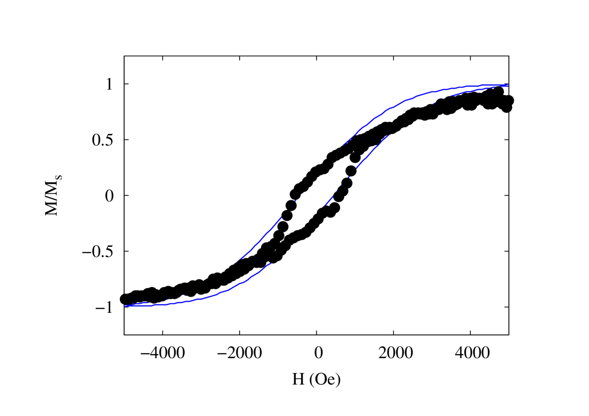
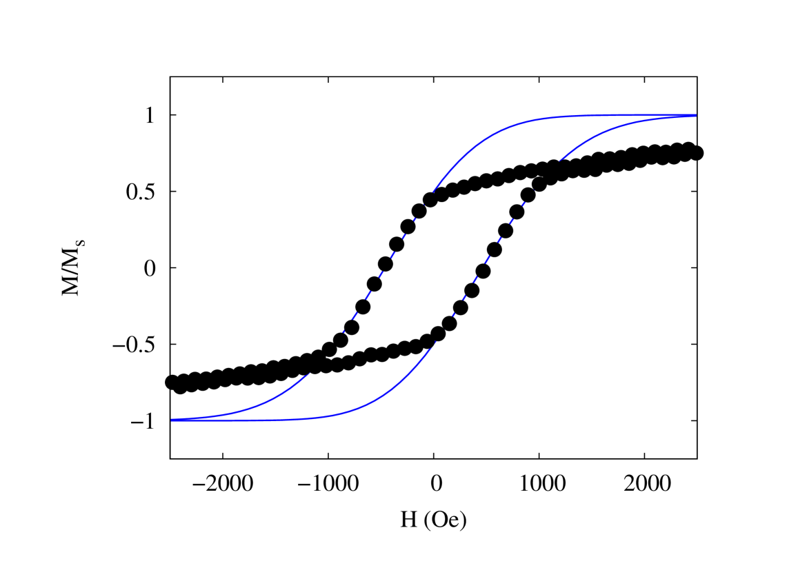
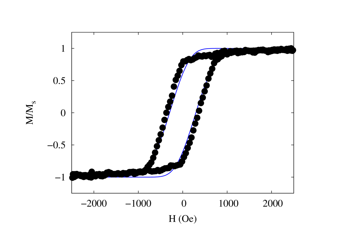
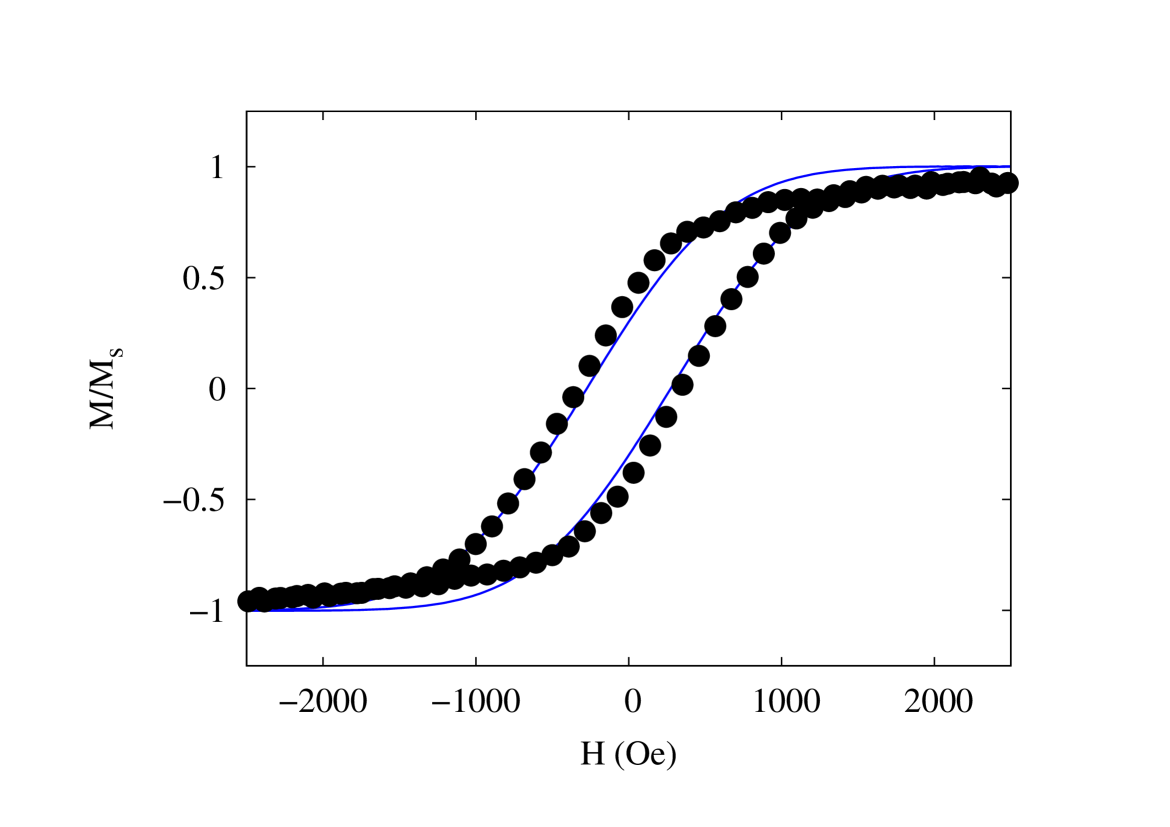
Loop inclination increases with $\sigma_{i}$ whereas loop width increases with $\sigma_{c}$. Hence interactions between ”hysterons” (or nanowires in our case) are responsible for the inclination observed in the VSM hysteresis loops. The fit parameters are given in table 1.

Table 1: Fitting parameters of the PM2 model of the hysteresis loops of Ni 15, 50, 80 and 100 nm diameter samples when external field $H$ is along nanowire axis i.e. $\theta_{H}=0$ (see fig. 1).

$d$(nm)	$H_{0}$ (Oe)	$h_{i0}$ (Oe)	$\sigma_{i}$ (Oe)	$\sigma_{c}$ (Oe)
15	120	600	1800	555
50	180	30	600	600
80	170	170	200	390
100	170	300	650	348

The coercivity parameter reflects presence of pinning centers hampering domain motions.

The Preisach fit is next made on the angular (between field and nanowire axis, see fig. 1) dependent hysteresis loops and we present in Table 2 the detailed results, as an example, for the 100 nm diameter case.

Table 2: Fitting parameters of the PM2 model of the hysteresis loops of Ni 100 nm diameter samples for several angles $\theta_{H}$ between external field $H$ and nanowire axis (see fig. 1).

Angle $\theta_{H}$	$H_{0}$ (Oe)	$h_{i0}$ (Oe)	$\sigma_{i}$ (Oe)	$\sigma_{c}$ (Oe)
0∘	170	300	650	348
30∘	170	200	750	360
45∘	170	100	900	345
60∘	100	50	1180	365
90∘	100	20	1300	450

One of the great advantages of the PM2 model is that the loop width is controlled by the standard deviation of the coercive fields $\sigma_{c}$ whereas its inclination is tunable by the standard deviation of the interaction fields $\sigma_{i}$. Once we fit the hysteresis loop we use the same parameters to evaluate the FMR lineshape as explained next.

III FMR lineshape versus angle

Individual wires inside the array are aligned parallel to each other within a deviation of a few degrees. They are characterized by a cylindrical shape with a typical variation in diameter of less than 5% with a low-surface roughness and a typical length of 6 microns.

FMR experiments are performed with the microwave pumping field $h_{rf}$ operating at 9.4 GHz with a DC bias field $H$ making a variable angle $\theta_{H}$ with the nanowire axis (through sample rotation).

Previously, several studies have considered reversal modes by domain nucleation and propagation (see for instance Henry et al. Henry for an extensive discussion of the statistical determination of reversal processes and distribution functions of domain nucleation and propagation fields). Moreover, Ferré et al. Ferre and Hertel Hertel showed the existence of domains with micromagnetic simulations). We do not consider domain nucleation and propagation in this work and rather concentrate on transverse single domain case.

Thus, the angular dependence of $H_{res}$ in the uniform mode is obtained by considering an ellipsoid with energy $E$ comprised of a small second-order effective uniaxial anisotropy cubic contribution ($K_{1}$ term in eq. 4) and (shape) demagnetization energy ($\pi M_{S}^{2}$ term in eq. 4 with $M_{S}$ the saturation magnetization). Their sum is the total anisotropy energy $E_{A}$ to which we add a Zeeman term $E_{Z}$ due to the external field $H$:

$$E=E_{A}+E_{Z}=(K_{1}+\pi M_{S}^{2})\sin^{2}\theta$$

$$-M_{S}H[\sin\theta\sin\theta_{H}\cos(\phi-\phi_{H})+\cos\theta\cos\theta_{H}]$$ (4)

$\theta$ is the angle the magnetization makes with the nanowire axis (see fig. 1).

The resonance frequency is obtained from the Smit-Beljers Smit formula that can be derived from the Landau-Lifshitz equation of motion with a damping term $\alpha$:

$$\left[{\frac{\omega}{\gamma}}\right]^{2}=\frac{(1+\alpha^{2})}{M_{S}^{2}\sin^{2}\theta}\left[{\frac{\partial^{2}E}{\partial\theta^{2}}\frac{\partial^{2}E}{\partial\phi^{2}}-\left({\frac{\partial^{2}E}{\partial\theta\,\partial\phi}}\right)^{2}}\right]$$ (5)

The frequency linewidth is given by:

$$\Delta\omega=\frac{\gamma\alpha}{M_{S}}\left({\frac{\partial^{2}E}{\partial\theta^{2}}+\frac{1}{\sin^{2}\theta}\frac{\partial^{2}E}{\partial\phi^{2}}}\right)$$ (6)

The frequency-field dispersion relation is obtained from the Smit-Beljers equation after evaluating the angular second derivatives Ebels of the total energy and taking $\phi=\phi_{H}=\frac{\pi}{2}$:

$$\frac{\omega}{\gamma}=\sqrt{(1+\alpha^{2})[H_{{eff}}\cos 2\theta+H\cos(\theta-\theta_{H})]}\times$$

$$\hskip 85.35826pt\sqrt{[H_{{eff}}\cos^{2}\theta+H\cos(\theta-\theta_{H})]}$$ (7)

At resonance, we have $\omega=\omega_{r}$, the resonance frequency, $\theta=\theta_{H}$ and the applied field $H=H_{res}$, the resonance field, when we are dealing with the saturated case. In the unsaturated case the magnetization angle $\theta\neq\theta_{H}$ and one determines it directly from energy minimization.

The above relation 7 provides a relationship between the effective anisotropy field $\bm{H}_{eff}$ and the external field $H$ at the resonance frequency.

Generally, the effective anisotropy field $\bm{H}_{eff}$ can be obtained from the vectorial functional derivative of the energy $E_{A}$ (eq. 4) with respect to magnetization $\bm{H}_{eff}~{}=~{}-\frac{\delta E_{A}}{\delta\bm{M}}$ that becomes in the uniform case the gradient with respect to the magnetization components $\bm{H}_{eff}~{}=~{}-\frac{\partial E_{A}}{\partial\bm{M}}$.

Moreover, we need to determine magnetization orientation $\theta_{0}$ at equilibrium. This is obtained from the minimum condition by evaluating the first derivative ${(\frac{\partial E}{\partial\theta})}_{\theta_{0}}=0$ and requiring positivity of the second derivative. Consequently, we get:

$$(K_{1}+\pi M_{S}^{2})\sin 2\theta_{0}=M_{S}\,H\,\sin\,\left({\theta_{H}-\theta_{0}}\right)$$ (8)

This equilibrium equation 8 and Smit-Beljers equation 7 are used simultaneously to determine the resonance field $H_{res}$ versus angle $\theta_{H}$ as analyzed next.

III.1 Analysis of the effective anisotropy field

In order to evaluate the total effective anisotropy field $H_{{eff}}$, we include in the energy $E_{A}$, demagnetization, magnetocrystalline anisotropy, and interactions among nanowires, with the corresponding fields $H_{dem}=2\pi M_{S}$, $H_{K}=\frac{2K_{1}}{M_{S}}$ and $H_{i}$, thus:

$$H_{{eff}}=H_{dem}+H_{i}+H_{K}$$ (9)

The interaction field $H_{i}$ comprises dipolar interactions between nanowires that depend on porosity $P$ (filling factor) and additional interactions as described in the CPM and PM2 models (see Appendix II). For example, if we consider the simplest case, demagnetization and dipolar fields are of the same form and may be written Ebels as a single term $2\pi M_{S}(1-3P)$.

Experimentally, the resonance field $H_{res}$ versus field angle $\theta_{H}$ peaks Encinas at $\omega_{r}/\gamma$, hence it is possible to extract the effective anisotropy field $H_{{eff}}$ through the use of eq. 7. Thus the Landé $g$-factor, saturation magnetization $M_{S}$ and cubic anisotropy constant $K_{1}$ can be determined with a least-squares fitting method Tannous similar to the one used in Appendix I.

This yields the following table 3 containing fitting parameters $K_{1}$ and $M_{S}$ (Anisotropy and saturation magnetization) versus diameter.

Table 3: Room temperature fitting parameters $K_{1}$ and $M_{S}$ with corresponding Nickel nanowire diameter $d$ and average separation $D$. Effective $H_{{eff}}$ and anisotropy $H_{K}$ fields are determined with Smit-Beljers. Comparing with bulk Nickel anisotropy aniso coefficient at room temperature: $K_{1}=-4.5\times 10^{4}$ erg/cm³ and saturation magnetization $M_{S}$=485 emu/cm³ we infer that as the diameter increases we get closer to the bulk values as expected with $K_{1}$ changing by about two orders of magnitude.

$d$	$D$	$K_{1}$	$M_{S}$	$H_{{eff}}$	$H_{K}$
(nm)	(nm)	(erg/cm3)	(emu/cm3)	(Oe)	(Oe)
15	256	-1.909 $\times$ 106	988.22	2344.58	-3864.61
50	510	-1.621 $\times$ 105	451.95	2122.17	-717.52
80	393	-2.424 $\times$ 105	453.25	1778.32	-1069.56
100	497	-8.037 $\times$ 104	410.24	2185.78	-391.81

From table 3, one infers that as the diameter increases the Ni bulk values are steadily approached which is a good test of the FMR fit.

III.2 Preisach modeling of FMR lineshape and transverse susceptibility

The FMR lineshape is obtained from the field derivative $\frac{d<\chi_{xx}^{{}^{\prime\prime}}>}{dH}$ of the average transverse susceptibility imaginary part $<\chi^{{}^{\prime\prime}}_{xx}>$ given by:

$$<\chi_{xx}^{{}^{\prime\prime}}>=\iint_{S}p(H_{\alpha},H_{\beta})\chi_{xx}^{{}^{\prime\prime}}dH_{\alpha}dH_{\beta}$$ (10)

The fields $H_{\alpha},H_{\beta}$ are the switching fields that define the Preisach plane (see Appendix II) over which the double integration above is performed in order to estimate the average.

The expression of the transverse susceptibility imaginary part is derived directly from the energy Dumitru and given by:

$$\chi_{xx}^{{}^{\prime\prime}}=\frac{\omega}{{(\omega_{r}^{2}-\omega^{2})}^{2}+\omega^{2}\Delta\omega_{r}^{2}}\times$$

$$\left[-\gamma^{2}(1+\alpha^{2})\left(\frac{\partial^{2}E}{\partial\theta^{2}}\right)\Delta\omega_{r}+\alpha\gamma M_{S}(\omega_{r}^{2}-\omega^{2})\right]$$ (11)

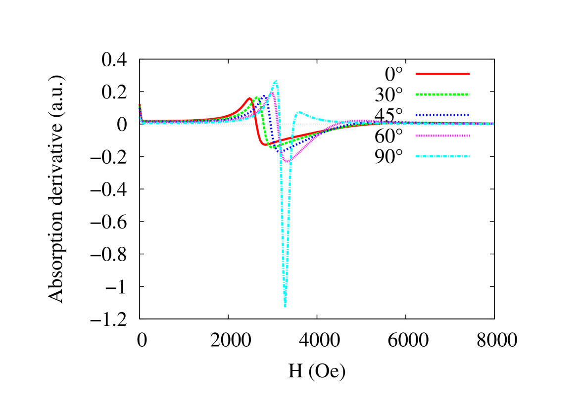
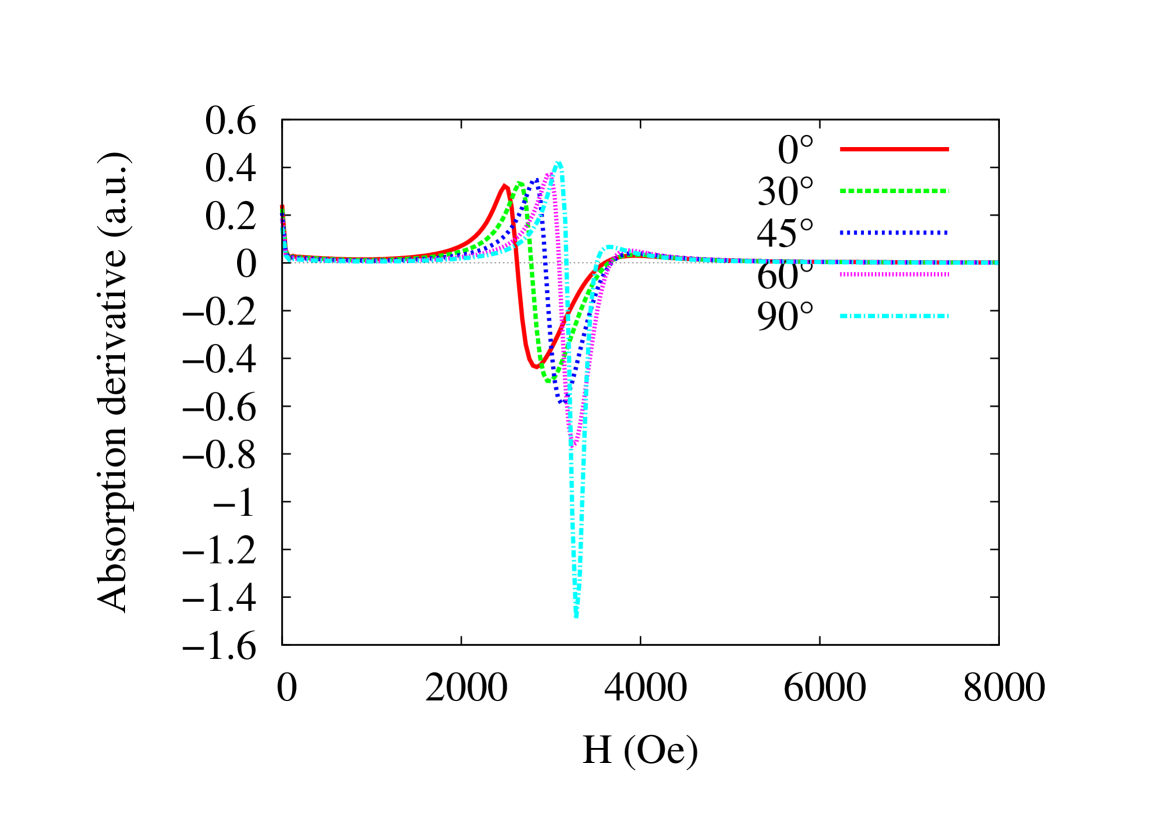
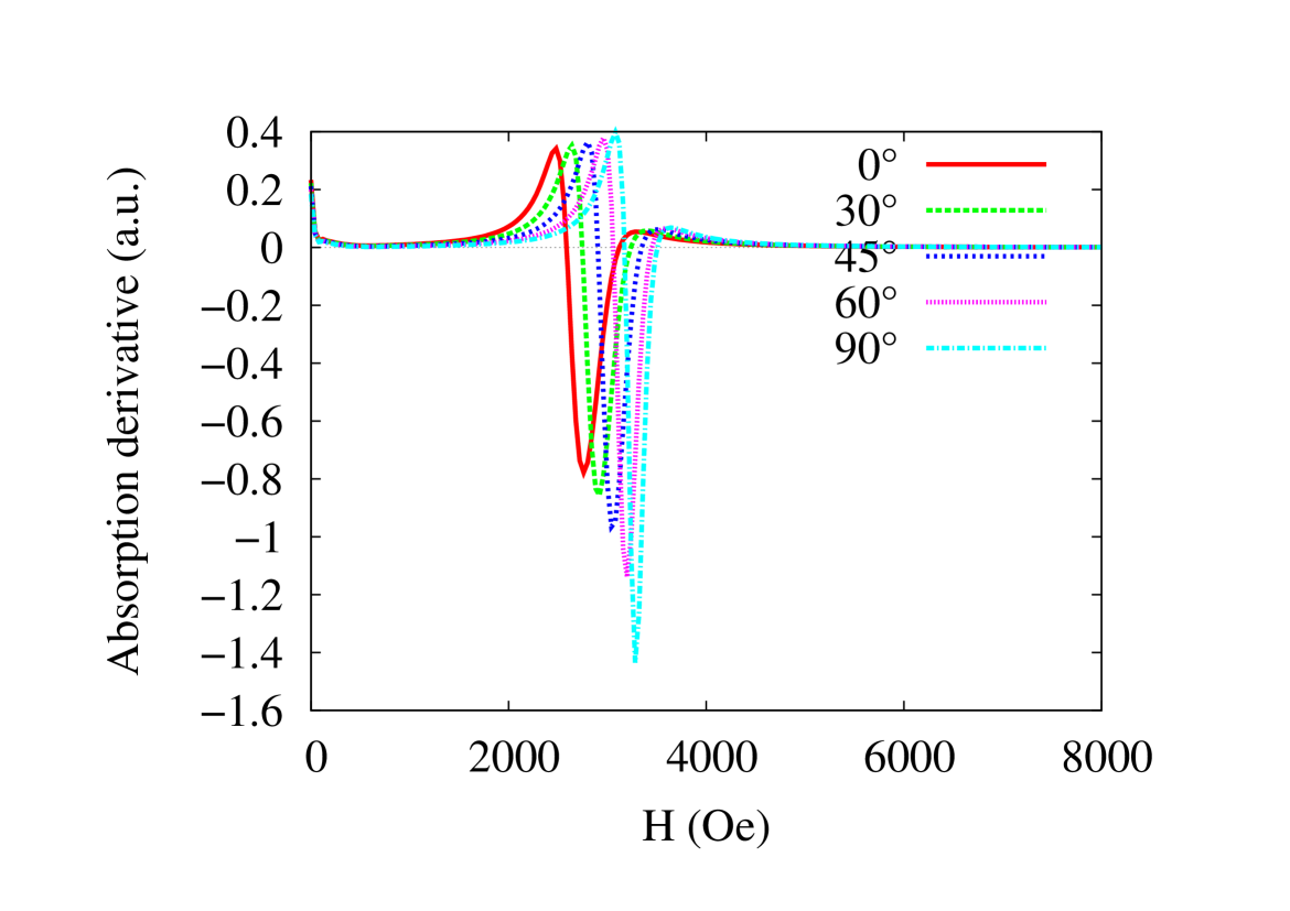
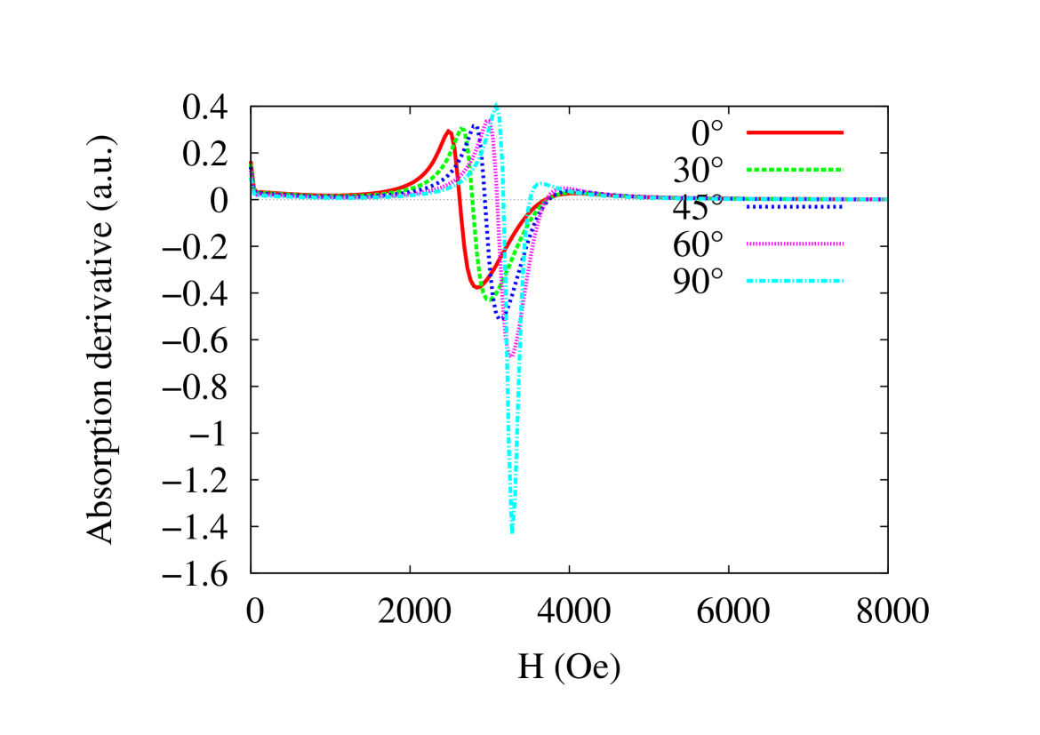
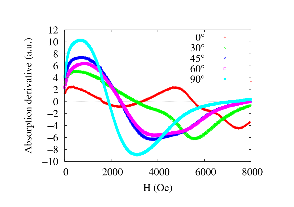
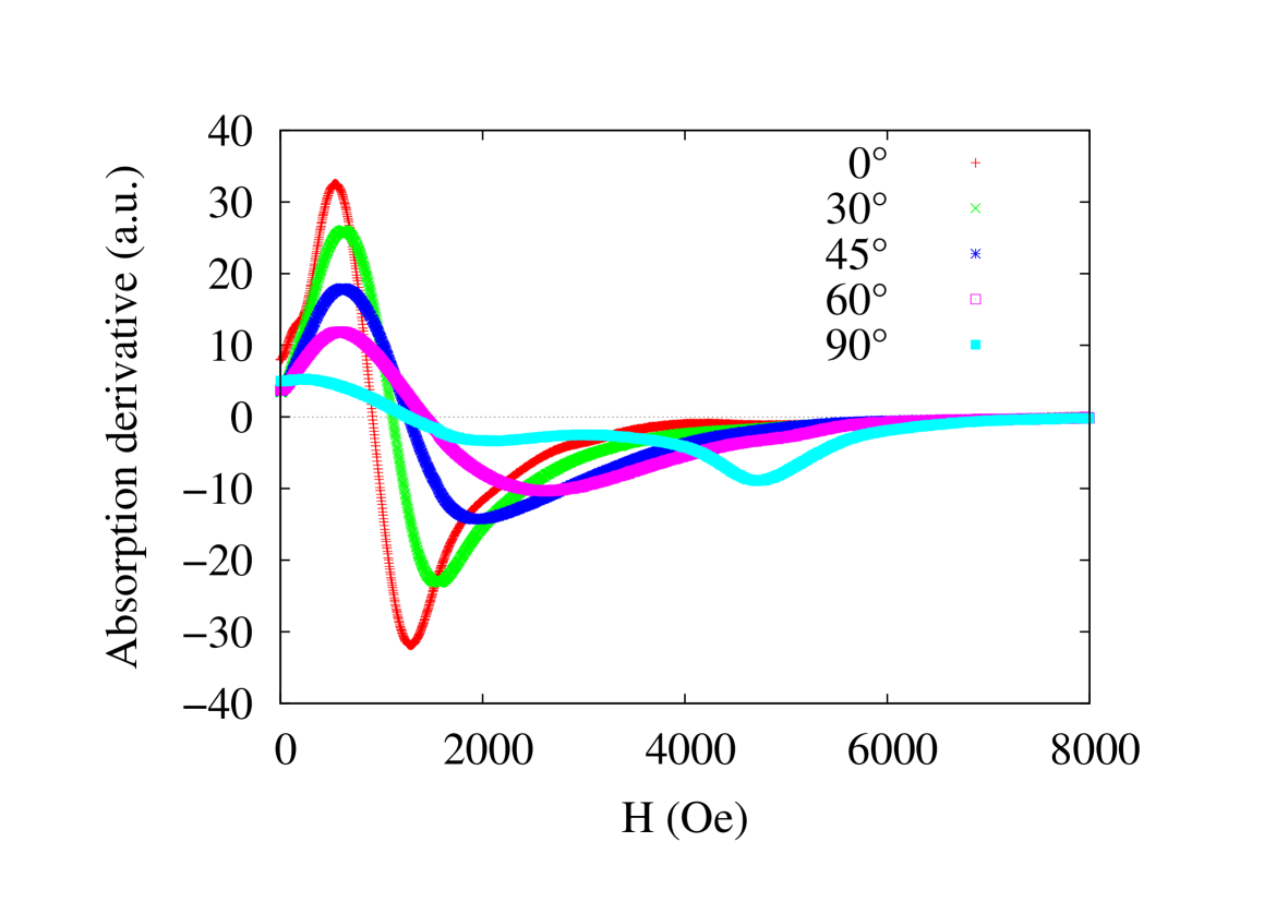
Performing the above double integral over the Preisach plane we spline the values obtained and take the derivative with respect to $H$ from the splined value (see for instance Numerical Recipes NR ). The results are displayed in fig. 3.

Figure 3: (Color on-line) Calculated derivative of the absorption $\frac{d<\chi_{xx}^{{}^{\prime\prime}}>}{dH}$ versus field for several field angles $\theta_{H}$ and all diameters. The Preisach parameters are the same used in the hysteresis loop fit. The lineshape is in arbitrary units and drawn for field angles of 0, 30, 45, 60 and 90 degrees, in all diameter cases: 15, 50, 80 and 100 nm (from top to bottom).

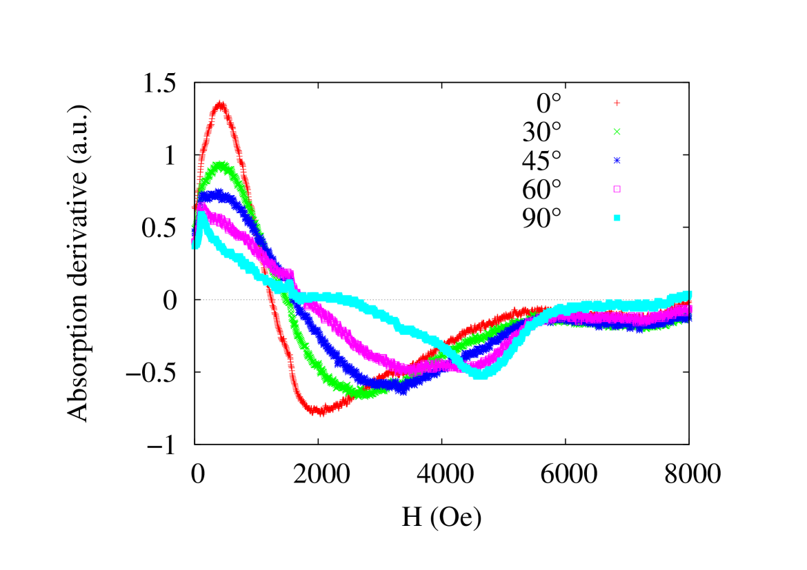
The FMR derivative spectrum is easily found to be asymmetric in contrast to what is normally obtained with Landau-Lifshitz-Gilbert modeling. The Preisach PM2 results agree with lineshapes previously obtained in the literature by Ebels et al. Ebels as well as Dumitru et al. Dumitru but not with our measurements (see fig. 4) that display a small field shift with angle $\theta_{H}$.

In table 4 we display results we obtain for the PM2 parameters that fitted the hysteresis loops and FMR measurements of $\chi_{xx}^{{}^{\prime\prime}}$ versus field in the Ni2 and Ni6 sample cases Dumitru . Note that some values of Table 4 are different from those given in Table I of ref. Dumitru , nevertheless it shows that the PM2 model is capable of achieving hysteresis loop and FMR results for the samples Ni2 and Ni6.

Table 4: Results obtained for PM2 model parameters belonging to samples Ni2 and Ni6 studied by Dumitru et al. Dumitru . We differ from some of the parameters displayed in their Table I.

Fields (Oe)	Field orientation	Ni2	Ni6
$H_{0}$	in wire plane	120	180
	perpendicular to wire plane	125	170
$h_{i0}$	in wire plane	1430	180
	perpendicular to wire plane	70	580
$\sigma_{i}$	in wire plane	260	720
	perpendicular to wire plane	250	610
$\sigma_{c}$	in wire plane	40	240
	perpendicular to wire plane	60	265

Turning to the calculated linewidths concerning our FMR measurements, we infer that they are smaller than the experimental values which implies that we have to include additional interactions in the dynamic (FMR) calculation. This is due to the fact we concentrate on the PM2 model with the same values of the parameters that previously fitted the hysteresis loops for all field angles. This contrasts with Dumitru et al. Dumitru who did the fit for two orientations of the field only ($\theta_{H}=$ 0^∘and 90^∘).

Moreover, let us point out from the $H_{res}$ versus $\theta_{H}$ fit (in Table 3) that in the dynamic case, several values, such as the anisotropy constant $K_{1}$ changes significantly, when diameter is reduced from 100 nm to 15 nm because of the appearance of surface anisotropy Tannous . Therefore a more complex Preisach model needed in order to fit static and dynamic results with the same sets of parameters for all angles.

Figure 4: (Color on-line) Measured FMR lineshape versus field for different angles with respect to nanowire axis at a frequency of 9.4 GHz and at room temperature. The lineshape $\frac{d<\chi_{xx}^{{}^{\prime\prime}}>}{dH}$ in arbitrary units is drawn for various angles $\theta_{H}=$ 0, 30, 45, 60 and 90 degrees, for 15, 50, 80 and 100 nm nanowire diameters (from top to bottom).

III.3 Angular Analysis of FMR lineshape width results

Measured FMR lineshapes (absorption derivative spectra Ebels ) for different angles are displayed in fig. 4 for 15 nm, 50 nm, 80 nm and 100 nm diameter cases. Generally the lineshapes behave versus magnetic field as the derivative of a Lorentzian.

We use a least-squares algorithm to extract the values of the Lorentzian widths as explained in Appendix I.

The width results displayed in Table 5 show that it is possible to relate unambiguously the value of the Lorentz derivative width to the angle $\theta_{H}$ for a given diameter, hence the possibility to build angle sensors on the basis of that observation.

Table 5: Lorentz derivative widths (in Oe), versus field angle $\theta_{H}$, fitted with respect to experimental angular FMR lineshapes pertaining to 15, 50, 80 and 100 nm diameter samples.

$d$(nm)	0∘	30∘	45∘	60∘	90∘
15	3557	2742	1806	1791	1364
50	1020	1120	1251	1495	2069
80	839	1092	1278	1349	2215
100	638	777	909	1100	1227

Lorentz derivative widths generally decrease as we increase nanowire diameter for all angles. For a fixed diameter, they increase with angle in the 50, 80 and 100 nm whereas in the 15 nm case they decrease. This originates from the fact, the 15 nm case possesses a large surface anisotropy as analysed previously in ref. Tannous , besides the lineshape behavior in this case is more complicated than the larger diameter cases.

IV Discussion and Conclusion

We have performed angular Preisach analysis for the static (VSM hysteresis loops) and dynamic measurements (FMR lineshape widths) and shown that many results can be deeply understood and might be further developed in order to be embedded in applications such as angle detection sensors.

The transition at 50 nm in VSM and FMR measurements is extremely promising because of several potential applications in race-track MRAM devices. Yan et al. Yan predicted that in Permalloy nanowires of 50 nm and less, moving zero-mass domain walls may attain a velocity of several 100 m/s beating Walker limit obeyed in Permalloy strips with same lateral size. Hence, nanowire cylindrical geometry in contrast to prismatic geometry of stripes bears important consequences on current injection in nanowires that applies Slonczewski type torques Kiselev on magnetization affecting domain wall motion with reduced Ohmic losses Tretiakov .

Ordered arrays of nanowires are good candidates for patterned media and may also be used in plasmonic applications such as nano-antenna arrays or nanophotonic waveguides in integrated optics plasmon . Recently Stipe , heat assisted magnetic perpendicular recording using plasmonic aperture nano-antenna has been tested on patterned media in order to process large storage densities starting at 1 Tbits/in² and scalable up to 100 Tbits/in².

While the Preisach PM2 model can explain separately the static or dynamic results, one might extend it through the use of other distributions of interaction and coercivity in order to explain the VSM and FMR measurements simultaneously for all angles.

Nonetheless, the angular behavior of the linewidth is interesting enough to consider its use in angle sensors that might compete with present technology based on AMR or GMR effects.

Appendix A Angular FMR linewidth evaluation procedure

We have developed a procedure based on a least squares minimization procedure of the curve $\frac{d\chi^{{}^{\prime\prime}}}{dH}$ versus $H$ to the set of $n$ experimental measurements ${[x_{i},~{}y_{i}]}_{i=1,n}$ where $x_{i}=H_{i}$ and $y_{i}=\frac{d\chi^{{}^{\prime\prime}}(\bm{\beta};x_{i})}{dH}$. $\bm{\beta}$ represents a set of fitting parameters.

One of the parameters is the width $\Delta H$ obtained from a fitting procedure to the derivative of a Lorentzian whose expression is given by:

$$\left[\frac{d\chi^{{}^{\prime\prime}}}{dH}\right]_{\mathscr{L}}=\frac{A(H-H_{0})}{({\Delta H}^{2}+(H-H_{0})^{2})^{2}}$$ (12)

$H_{0}$ is not a fitting parameter since it can be determined by the intersection of the lineshape with the $H$ axis. The parameters $A,\Delta H$ are determined with a fitting procedure. Writing the set of minima equations to be satisfied at the data points:

$$\frac{1}{n}\sum_{i=1}^{n}\left\{\left[\frac{d\chi^{{}^{\prime\prime}}(\bm{\beta};x_{i})}{dH}\right]_{\mathscr{L}}-y_{i}\right\}^{2}\mbox{ minimum},\\$$

The fitting method is based on the Broyden algorithm, a generalization to higher dimension of the one-dimensional secant method NR that allows us to determine in a least-squares fashion, the set of unknowns $A,\Delta H$. Broyden method is selected because it can handle over or under-determined numerical problems and that it works from a singular value decomposition point of view NR . This means it is able to circumvent singularities and deliver a practical solution to the problem at hand as an optimal setNR within a minimal distance from the real one.

Appendix B Preisach formalism overview

Preisach model mayergoyz91 is based on a statistical approach towards magnetization processes mayergoyz91 , bertotti98 .

Comparing Preisach formalism and micromagnetics is akin to understanding the link between thermodynamics and statistical mechanics.

The nanowire array is viewed as made of single domain interacting entities each nanowire being represented by a switching field and a local interaction field. The local interaction field in each nanowire is assumed to be constant. A system of interacting nanowires is represented by a probability density function (PDF) $p(h_{i},h_{c})$ depending on interaction and coercive fields $H_{i}$ and $H_{c}$ respectively.

The main objective in Preisach modeling is to find the best $p(h_{i},h_{c})$ such that the best possible agreement with system behavior is obtained.

Preisach formalism is an energy-based description of hysteresis, and does not require that the material under investigation be decomposable into discrete physical entities such as magnetic particles.

It assumes that the magnetic system free energy functional can be decomposed into an ensemble of elementary two level (double well) subsystems (TLS)mayergoyz91 .

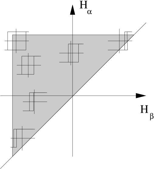
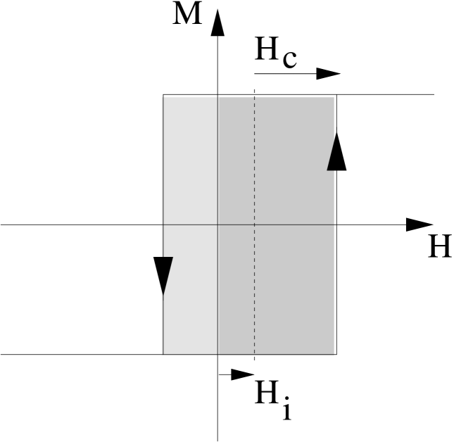
It represents the magnetic material into a collection of microscopic bistable units ”hysterons” having statistically distributed coercive and interaction fields. Each unit is characterized by a rectangular hysteresis loop (see fig. 5) and its status is determined by the actual field and history of the applied external fields.

The classical version (CPM) of the model is based on the use of a joint distribution of normalized interaction fields $H_{i}$ and coercive fields $H_{c}$. The interaction fields $H_{i}$ induce a shift in the elementary hysteresis loop (see fig. 5) whereas the coercive fields increase its width. Integrating the density over a given path in the Preisach plane yields a magnetization process.

These fields originate from the existence of switching fields $(H_{\alpha},H_{\beta})$ that span the Preisach plane (see fig. 5) such that:

$$H_{\alpha}=H_{i}+H_{c},\hskip 5.69046ptH_{\beta}=H_{i}-H_{c},$$

$$H_{i}=\frac{H_{\alpha}+H_{\beta}}{2},\hskip 5.69046ptH_{c}=\frac{H_{\alpha}-H_{\beta}}{2}$$ (13)

Mayergoyz mayergoyz91 has demonstrated that the necessary and sufficient conditions for a system to be rigorously described by a CPM are the wiping-out and congruency properties Stancu . A hysteretic system will present the wiping-out property when it returns to the same state after performing a minor loop. The second property refers to the shape of the minor loops measured in the same field range; if all these minor loops are congruent within a given field range and this property does not depend on the actual field range used in the experiment, the system obeys the congruency property.

Figure 5: (a) Preisach ($H_{\alpha},H_{\beta}$) plane displaying different hysteresis loops at different locations. At each point an elementary hysteresis loop is displayed characterized by the values of the interaction $H_{i}$ and coercive $H_{c}$ fields. (b) An elementary hysteron with a square hysteresis loop is shown shifted by the interaction field $H_{i}$ and possessing a half-width given by the coercive field $H_{c}$.

The major hysteresis loop is obtained when a path linear in the applied field is used mayergoyz91 , bertotti98 . Thus, in order to estimate the the hysteresis loop, we determine the magnetization $M$ with a double integration over the PDF as given below:

$$M=2M_{S}\int_{0}^{\infty}dh_{i}\int_{0}^{b(h_{i})}dh_{c}p(h_{i},h_{c})$$ (14)

where the function $b(h_{i})$ represents such path.

The $H_{i},H_{c}$ PDF can be either analytically built from standard PDF (Gaussian, Lorentzian, uniform etc…) or experimentally determined from FORC (First Order Reversal Curves) measurements. This originates from the fact magnetic interactions between nanowires are a major determinant of noise levels in magnetic media whether it is used for storage or processing such as in spintronics.

While conventional methods of characterizing magnetic interactions utilize Isothermal Remanent Magnetization (IRM) and remanence DC Demagnetization (DCD) curves mayergoyz91 , Preisach modeling is based on some distribution which is supposed to adequately describe the magnetic system at hand.

FORC is a popular measurement leading to an appropriate Preisach model. It begins with sample saturation with a large positive field. The field is ramped down to a reversal field $H_{\alpha}$. FORC consists of a measurement of the magnetization as the field is then increased from $H_{\alpha}$ back up to saturation. The magnetization at applied field $H_{\beta}$ on the FORC with reversal point $H_{\alpha}$ is denoted by $M(H_{\alpha},H_{\beta})$, where $H_{\beta}\geq H_{\alpha}$ .

The PDF is obtained from the second mixed derivative:

$$p(H_{\alpha},H_{\beta})=-\frac{\partial^{2}M}{\partial H_{\alpha}\partial H_{\beta}}$$ (15)

Let us assume we adopt a double Lorentzian PDF given by:

$$p(h_{i},h_{c})=\frac{2}{\pi\sigma^{2}_{i}H^{2}_{0}[\frac{\pi}{2}+\tan^{-1}(\frac{1}{\sigma_{i}})]}\times$$

$$\frac{1}{[1+(\frac{h_{i}+h_{c}-H_{0}}{\sigma_{i}H_{0}})^{2}][1+(\frac{h_{i}-h_{c}-H_{0}}{\sigma_{i}H_{0}})^{2}]}$$ (16)

with $h_{i},h_{c}$ a set of normalized fields, $\sigma_{i},\sigma_{c}$ the standard deviation of the individual Lorentzian/Gaussian distributions considered as independent) we find hysteresis loops that are upstraight whereas the VSM measured loops exhibit some inclination.

When one uses rather a double Gaussian PDF as in the CPM case, we get inclined hysteresis loops as observed with the VSM measurements.

Nevertheless both approaches do not agree with the hysteresis loops that we find experimentally as described by Dumitru et al. Dumitru . This is why we use the PM2 model as explained in section II.

References

- (1) A Singh, S Mukhopadhyay and A Ghosh, Phys. Rev. Lett. 105, 067206 (2010).
- (2) A Singh and A Ghosh, Phys. Rev. B 84, 060407(R) (2011).
- (3) Z. Z. Sun and J. Schliemann, Phys. Rev. Lett. 104, 037206 (2010).
- (4) M. Yan, A. Kakay, S. Gliga and R. Hertel, Phys. Rev. Lett. 104, 057201 (2010).
- (5) C. T. Boone, J. A. Katine, M. Carey, J. R. Childress, X. Cheng, and I. N. Krivorotov, Phys. Rev. Lett. 104, 097203 (2010).
- (6) V. V. Kruglyak, S. O. Demokritov and D. Grundler, J. Phys. D: Appl. Phys. 43, 264001 (2010).
- (7) Coupling GHz range electromagnetic waves (with 30 cm) to nanowires of diameter 100 nm must respect the cutoff condition . Devices using surface plasmons may be used to inject electromagnetic energy through nanowires (see for instance Ditlbacher et al. plasmon ).
- (8) J. K. W. Yang, E. Dauler, A. Ferri, A. Pearlman, A. Verevkin, G. Gol’tsman, B. Voronov, R. Sobolewski, W. E. Keicher and K. K. Berggren, IEEE Trans. App. Superconductivity, 15, 626 (2005).
- (9) A. Fert, Rev. Mod. Phys. 80, 1517 (2008), P. Grünberg Rev. Mod. Phys. 80, 1531 (2008).
- (10) Electrochemical methods have been extensively described in the literature and a recent review on the subject would be for instance G. Kartopu, O. Yalçin, K.-L. Choy, R. Topkaya, S. Kazan, and B. Aktaş, J. Appl. Phys. 109, 033909 (2011) or H. Pan, B. Liu, J. Yi, C. Poh, S. Lim, J. Ding, Y. Feng, C. H. A. Huan and J. Lin, J. Phys. Chem. B 109, 3094 (2005).
- (11) C. Tannous, A. Ghaddar and J. Gieraltowski, Appl. Phys. Lett. 100, 182401 (2012).
- (12) A. Klein, A. Schmidt, W. Meyer, L. Hammer, and K. Heinz Phys. Rev. B 81, 115431 (2010).
- (13) S. Y. Chou, Proceedings of the IEEE, 85, 652 (1997).
- (14) Y. Henry, A. Iovan, J.-M. George and L. Piraux, Phys. Rev. B. 66, 184430 (2002).
- (15) R. Ferré, K. Ounadjela, J. M. George, L. Piraux and S. Dubois, Phys. Rev. B. 56, 14066 (1997).
- (16) R. Hertel, J. Appl. Phys. 90, 5752 (2001).
- (17) In spite of the fact bulk Nickel has cubic anisotropy aniso , our description based on uniaxial anisotropy is sufficient Wegrowe to describe the FMR spectra. For a description based on a cubic anisotropy see De La Torre Medina et al. Darques .
- (18) L. Baselgia, M. Warden, F. Waldner, Stuart L. Hutton, John E. Drumheller, Y. Q. He, P. E. Wigen, and M. Marys̆ko, Phys. Rev. B 38, 2237 (1988).
- (19) U. Ebels, J. Duvail, P. Wigen, L. Piraux, L. D. Buda, K. Ounadjela, Phys. Rev. B 64, 144421 (2001).
- (20) A. Encinas, M. Demand, L. Vila, L. Piraux, and I. Huynen, Appl. Phys. Lett. 81, 2032 (2002).
- (21) Cubic anisotropy energy to sixth-order is: where: are the cosines of the angles, the magnetization makes with the axes respectively (see fig. 1). At room temperature, bulk Nickel values are: erg/cm3, erg/cm3 and =485 emu/cm3.
- (22) I. Dumitru, F. Li, J. B. Wiley, D. Cimpoesu, A. Stancu and L. Spinu IEEE Trans. Mag. 42 3225 (2006), see also L. Spinu, I. Dumitru, A. Stancu and D. Cimpoesu JMMM 296, 1 (2006).
- (23) W. H. Press, W. T. Vetterling, S. A. Teukolsky and B. P. Flannery, ”Numerical Recipes in C: The Art of Scientific Computing”, Second Edition, Cambridge University Press (New-York, 1992).
- (24) S. I. Kiselev, J. C. Sankey, I. N. Krivorotov, N. C. Emley, R. J. Schoelkopf, R. A. Buhrman and D. C. Ralph, Nature 425, 380 (2003) .
- (25) O. A. Tretiakov, Y. Liu, and A. Abanov, Phys. Rev. Lett. 105, 217203 (2010).
- (26) H. Ditlbacher, A. Hohenau, D. Wagner, U. Kreibig, M. Rogers, F. Hofer, F. R. Aussenegg and J. R. Krenn, Phys. Rev. Lett. 95, 257403 (2005).
- (27) B. C. Stipe, T. C. Strand, C. C. Poon, H. Balamane, T. D. Boone, J. A. Katine, J-L Li, V. Rawat, H. Nemoto, A. Hirotsune, O. Hellwig, R. Ruiz, E. Dobisz, D. S. Kercher, N. Robertson, T. R. Albrecht and B. D. Terris, Nature Photonics 4, 484 (2010).
- (28) I. D. Mayergoyz, Mathematical models of hysteresis (Springer-Verlag, New-York, 1991), see also R.B. Gorbet, Control of Hysteretic Systems with Preisach Representations, PhD Thesis, University of Waterloo (Ontario, CANADA 1997).
- (29) G. Bertotti, Hysteresis in Magnetism (Academic Press, San Diego, 1998).
- (30) L. Stoleriu, A. Stancu, L. Mitoseriu, D. Piazza and C. Galassi, Phys. Rev. B 74, 174107 (2006).
- (31) J-E Wegrowe, D. Kelly, A. Franck, S.E. Gilbert and J-Ph. Ansermet Phys. Rev. Lett. 82, 3681 (1999).
- (32) J. De La Torre Medina, M. Darques and L. Piraux, J. Phys. D: Appl. Phys. 41, 032008 (2008).