Preprocess the Photospheric Vector Magnetograms for NLFFF Extrapolation using a Potential Field Model and an Optimization Method

Abstract

Numerical reconstruction/extrapolation of coronal nonlinear force-free magnetic field (NLFFF) usually takes the photospheric vector magnetogram as input at the bottom boundary. Magnetic field observed at the photosphere, however, contains force which is in conflict with the fundamental assumption of the force-free model and measurement noise which is unfavorable for practical computation. Preprocessing of the raw magnetogram has been proposed by Wiegelmann, Inhester, and Sakurai (2006) to remove the force and noise for providing better input for NLFFF modeling. In this paper we develop a new code of magnetogram preprocessing which is consistent with our extrapolation method CESE–MHD–NLFFF (Jiang, Feng, and Xiang, 2012; Jiang and Feng, 2012a). Basing on a magnetic-splitting rule that a magnetic field can be split into a potential field part and a non-potential part, we split the magnetogram and deal with the two parts separately. Preprocessing of the magnetogram’s potential part is based on a numerical potential field model, and the non-potential part is preprocessed using the similar optimization method of Wiegelmann, Inhester, and Sakurai (2006). The code is applied to the SDO/HMI data and results show that the method can remove efficiently the force and noise and improve the quality of extrapolation.

1 Introduction

sec:intro

Magnetic field extrapolation is an important tool to study the three-dimensional (3D) solar coronal magnetic field, which is difficult to measure directly (Sakurai, 1989; Aly, 1989; Amari et al., 1997; McClymont, Jiao, and Mikic, 1997; Wiegelmann, 2008; DeRosa et al., 2009). The models being used most popularly for field extrapolation are the potential field model, the linear force-free field model, and the nonlinear force-free field (NLFFF) model. These models are all based on the same assumption that the Lorentz force is self-balancing in the corona, but adopt different simplifications of the current distribution. Among these models, the NLFFF model is the most precise one for characterizing magnetic field in the low corona, where there is significant and localized electric current, especially in active regions.

Regarding the NLFFF extrapolation, it is routine to use the vector magnetograms observed on the photosphere as input, at least in most of the available extrapolation codes (e.g., Wheatland, Sturrock, and Roumeliotis, 2000; Wiegelmann, 2004; Amari, Boulmezaoud, and Aly, 2006; Valori, Kliem, and Fuhrmann, 2007; Jiang and Feng, 2012a; Jiang, Feng, and Xiang, 2012; Inoue et al., 2011). This, however, poses a basic problem (also a major headache) to the force-free field modelers, because the magnetic field in the photosphere is forced by the plasma significantly (Metcalf et al., 1995), which is in conflict with the fundamental assumption of force-freeness. From the photosphere to the corona, the magnetic field passes through a highly stratified and inhomogeneous plasma environment with plasma $\beta$ varying abruptly from $>1$ to $\ll 1$ (Gary, 2001); thus the force-free condition cannot be fulfilled globally. By a study of the observed chromospheric field in a sampled active region, Metcalf et al. (1995) conclude that the magnetic field is not force-free in the photosphere, but becomes force-free roughly $400$ km above the photosphere. A recent statistical study by Liu et al. (2012) using a large number of magnetograms from Huairou Solar Observing Station gives similar conclusions.

This complication leads to the desire to use measurements of the vector field in the force-free upper chromosphere instead. However, the vector field is not as easily measured in the chromosphere as in the photosphere. Even the chromospheric field is measured, it is still problematic for extrapolation since the surface in which any particular magnetically-sensitive line will form varies in time and space, and in particular the height will be different along different lines of sight. So one cannot assume that the vector field is given on a plane or sphere at the bottom of the extrapolation volume as in the case of the photospheric magnetograms. The practical use of the chromospheric magnetograms as boundary conditions for extrapolations is still to be explored.

As an alternative way to alleviate the problem, one can consider to modify the photospheric magnetograms to simulate the force-free chromospheric magnetograms, which is first suggested by Wiegelmann, Inhester, and Sakurai (2006). Since the interface between the photosphere and the bottom of the force-free domain is rather thin (say, about 400 km), especially if compared with the spatial scale of the coronal field (about tens of megameters), the basic field structures of the chromosphere should be very similar to those of the photosphere, except that (i) there must be some smoothness of the structures due to the fast expansion of field from the high-$\beta$ to low-$\beta$ regions and (ii) the very fine magnetic elements are just closed within this interface and thus show no signal in the force-free domain. Thanks to these reasons, modifications that need to be made on the photospheric field to mimic the force-free chromospheric field ought to be not significant and can hopefully be made within/around the error margins of the measurement.

The procedure of modifying a raw photospheric magnetogram to a force-free chromospheric one is usually called ‘preprocessing’ (Wiegelmann and Neukirch, 2006; Fuhrmann, Seehafer, and Valori, 2007; Metcalf et al., 2008; Fuhrmann et al., 2011; Yamamoto and Kusano, 2012). To guide the preprocessing, there are constraints that must be fulfilled by the target magnetogram. On the boundary surface $S$ of an ideally force-free field ${\mathbf{B}}$ in a volume $V$, the field satisfies the following necessary conditions

eq:m1$$F_{x}=\int_{S}B_{x}B_{z}{\ \mathrm{d}}x{\ \mathrm{d}}y=0,\ \ F_{y}=\int_{S}B_{y}B_{z}{\ \mathrm{d}}x{\ \mathrm{d}}y=0,$$

$$F_{z}=\int_{S}E_{B}{\ \mathrm{d}}x{\ \mathrm{d}}y=0,\ \ T_{x}=\int_{S}yE_{B}{\ \mathrm{d}}x{\ \mathrm{d}}y=0,\ \ T_{y}=\int_{S}xE_{B}{\ \mathrm{d}}x{\ \mathrm{d}}y=0,$$

$$T_{z}=\int_{S}(yB_{x}B_{z}-xB_{y}B_{z}){\ \mathrm{d}}x{\ \mathrm{d}}y=0.$$ (1)

where $E_{B}=B_{x}^{2}+B_{y}^{2}-B_{z}^{2}$. These expressions are derived from the volume integrals of the total magnetic force and torque (Aly, 1989; Sakurai, 1989; Tadesse, 2011)

eq:m11$${\mathbf{0}}=\int_{V}{\mathbf{j}}\times{\mathbf{B}}{\ \mathrm{d}}V=\int_{V}\nabla\cdot{\mathbf{T}}{\ \mathrm{d}}V=\int_{S}{\mathbf{T}}{\ \mathrm{d}}{\mathbf{S}},$$

$${\mathbf{0}}=\int_{V}{\mathbf{r}}\times({\mathbf{j}}\times{\mathbf{B}}){\ \mathrm{d}}V=\int_{V}\nabla\cdot{\mathbf{T}}^{\prime}{\ \mathrm{d}}V=\int_{S}{\mathbf{T}}^{\prime}{\ \mathrm{d}}{\mathbf{S}}$$ (2)

where ${\mathbf{T}}$ is magnetic stress tensor,

$${\mathbf{T}}_{ij}=-\frac{{\mathbf{B}}^{2}}{2}\delta_{ij}+B_{i}B_{j}$$ (3)

and ${\mathbf{T}}_{ij}^{\prime}=\epsilon_{ikl}r_{k}{\mathbf{T}}_{lj}$. Generally the surface integration has to be carried out over a closed volume, but in preprocessing magnetograms for extrapolation of a computational cube, the surface integrals of Equation (eq:m11) is usually restricted within the bottom magnetogram since the contribution from other (side and top) boundaries is small and negligible, and in the following $S$ will represent only the area of magnetograms. With this assumption, Equation (eq:m1) is the component form of the surface integrals in Equation (eq:m11). So the first task of preprocessing is to drive the raw magnetogram to fulfill the constraints of Equation (eq:m1) and thus to be closer to an ideally force-free magnetogram. This task is also dubbed as ‘removing force’ in the forced magnetogram. The second task of preprocessing is to smooth the raw data to mimic the field expansion. Smoothing is also very necessary for the practical computation based on numerical difference with limited resolution, which cannot resolve sufficiently small structures in the raw data. Besides, smoothing can remove measurement noise and increase signal-to-noise ratio.

Several preprocessing codes (Wiegelmann, Inhester, and Sakurai, 2006; Fuhrmann, Seehafer, and Valori, 2007; Metcalf et al., 2008) have been developed and they share the basic approach proposed by Wiegelmann, Inhester, and Sakurai (2006). A functional $L$ is designed by adding up the $\chi^{2}$ deviations from the constraints of Equation (eq:m1), the terms that control deviation from the raw data and the smoothness with different weights, e.g.,

$$\ilabel{eq:L}L=\mu_{1}L_{1}+\mu_{2}L_{2}+\mu_{3}L_{3}+\mu_{4}L_{4}$$ (4)

where $\mu$ is the weighting factor, $L_{1}=F_{x}^{2}+F_{y}^{2}+F_{z}^{2}$, $L_{2}=T_{x}^{2}+T_{y}^{2}+T_{z}^{2}$, $L_{3}=\int_{S}|{\mathbf{B}}-{\mathbf{B}}_{\rm obs}|^{2}{\ \mathrm{d}}s$, and $L_{4}$ measures the roughness of the data. Then the target magnetogram is searched by minimizing the functional $L$ using an optimization method. Different algorithms of smoothing and optimization have been utilized and the results are more or less different, as shown in a comparison study by Fuhrmann et al. (2011). Also the differences can result from different choices of the weighting factors.

Under this framework of preprocessing, there are two problems not well addressed, namely, to what extent the force is needed to be removed and to what extent the smoothing can be performed? We care about these problems from both numerical and physical considerations. Ideally we prefer the map to satisfy the force-free constraints precisely, but this condition need not be satisfied strictly considering that numerical discretization error is unavoidable in the extrapolation with finite resolution. The smoothing also ought not to be done arbitrarily if we want to mimic the expansion of the field from the photosphere to some specific height above. Over-smoothing of the data may smear the basic structures while a too-limited smoothing cannot filter the small-scale noise sufficiently. A careful choice of the weighting factors $\mu$ is required to deal with these problems.

This paper is devoted to handling these problems in the preprocessing. We use the values of force-freeness and smoothness calculated from numerical potential-field solution at some height above the photosphere as a reference to guide the preprocessing. Based on a simple rule that any magnetic field can be split into two parts: a potential field and a non-potential field, we develop a new preprocessing code using this splitting of the magnetic field, which is consistent with our extrapolation code CESE–MHD–NLFFF (Jiang and Feng, 2012a; Jiang, Feng, and Xiang, 2012). We show below how the raw magnetogram can be driven to force-free and smooth with the same level as that of the numerical potential field at a height of roughly 400 km above the photosphere, i.e., the bottom of the force-free domain. The remainder of the paper is organized as follows. In Section sec:method we give the basic method and formulas, and we show how to choose the weighting factors in Section sec:mu. We then apply the method to preprocess two sampled magnetograms taken by SDO/HMI and analyze the results in Section sec:res. Finally discussion and conclusions are given in Section sec:con.

2 Method

sec:method

Generally the coronal magnetic field can be split into two parts: a potential field matching the normal component of the bottom magnetogram, and a non-potential part with the normal field vanishing at the bottom. Particularly, of the vector magnetogram, the magnetic field ${\mathbf{B}}$ can be written as

$${\mathbf{B}}={\mathbf{B}}_{0}+{\mathbf{B}}_{1}=(B_{0x}+B_{1x},B_{0y}+B_{1y},B_{0z})$$ (5)

where $(B_{0x},B_{0y},B_{0z})$ are the components of the potential part ${\mathbf{B}}_{0}$ and $(B_{1x},B_{1y})$ the components of the non-potential part ${\mathbf{B}}_{1}$. Note that $B_{0z}=B_{z}$ and $B_{1z}=0$.

Supposing ${\mathbf{B}}$ is a force-free magnetogram and since its potential part ${\mathbf{B}}_{0}$ already fulfills the force-free conditions of Equation (eq:m1), we can derive special force-free conditions for its non-potential part $(B_{1x},B_{1y})$, which are expressed as

eq:m3$$\int_{S}B_{1x}B_{0z}{\ \mathrm{d}}x{\ \mathrm{d}}y=0,\ \ \int_{S}B_{1y}B_{0z}{\ \mathrm{d}}x{\ \mathrm{d}}y=0,$$

$$\int_{S}\Gamma_{B}{\ \mathrm{d}}x{\ \mathrm{d}}y=0,\ \ \int_{S}x\Gamma_{B}{\ \mathrm{d}}x{\ \mathrm{d}}y=0,\ \ \int_{S}y\Gamma_{B}{\ \mathrm{d}}x{\ \mathrm{d}}y=0,$$

$$\int_{S}(yB_{1x}B_{0z}-xB_{1y}B_{0z}){\ \mathrm{d}}x{\ \mathrm{d}}y=0$$ (6)

where we denote $\Gamma_{B}=B_{1x}^{2}+B_{1y}^{2}+2(B_{0x}B_{1x}+B_{0y}B_{1y})$. The derivation is straightforward, for example

$$E_{B}=(B_{0x}+B_{1x})^{2}+(B_{0y}+B_{1y})^{2}-B_{0z}^{2}$$

$$=E_{B_{0}}+B_{1x}^{2}+B_{1y}^{2}+2(B_{0x}B_{1x}+B_{0y}B_{1y})=E_{B_{0}}+\Gamma_{B},$$ (7)

and we have

$$\int_{S}\Gamma_{B}{\ \mathrm{d}}x{\ \mathrm{d}}y=\int_{S}E_{B}{\ \mathrm{d}}x{\ \mathrm{d}}y-\int_{S}E_{B_{0}}{\ \mathrm{d}}x{\ \mathrm{d}}y=0.$$ (8)

All other expressions in Equation (eq:m3) can be derived easily in the similar way.

Let $\mathcal{B}~{}(\mathcal{B}_{x},\mathcal{B}_{y},\mathcal{B}_{z})$ denote the observed photospheric field, i.e., the raw magnetogram, and its splitting form is

$$\mathcal{B}=\mathcal{B}_{0}+\mathcal{B}_{1}=(\mathcal{B}_{0x}+\mathcal{B}_{1x},\mathcal{B}_{0y}+\mathcal{B}_{1y},\mathcal{B}_{0z})$$ (9)

with $\mathcal{B}_{0}$ and $\mathcal{B}_{1}$ denoting the potential and non-potential parts, respectively. Here $\mathcal{B}_{0}$ is computed based on $\mathcal{B}_{z}$ using the potential field model and then $\mathcal{B}_{1}$ is also obtained. The computation of a potential field needs only the normal component of the field on the bottom and is now a trivial task, which can be carried out conveniently by using the Green’s function method (Metcalf et al., 2008) or other much faster scheme (Jiang and Feng, 2012b).

Generally, $\mathcal{B}_{1}$ does not fulfill the force-free conditions of Equation (eq:m3). If without smoothing, we only need to let ${\mathbf{B}}_{0}=\mathcal{B}_{0}$ and reduce the non-potential part $\mathcal{B}_{1}$ to ${\mathbf{B}}_{1}$ satisfying Equation (eq:m3). For the purpose of smoothing, ${\mathbf{B}}_{0}$ is obtained by taking the data at a plane just one pixel above the photosphere from the 3D potential field extrapolated from the observed $\mathcal{B}_{0z}$. This is suitable for the SDO/HMI data which has a pixel size of about 360 km (i.e., 0.5 arcsec), an approximate height above which the coronal field becomes force-free according to Metcalf et al. (1995). For magnetograms with other sizes of pixel, we need to take the potential field data at a given physical height (where the force-free assumption becomes valid, e.g., 400 km) and not necessarily one pixel above the photosphere. ${\mathbf{B}}_{0}$ obtained in this way can be regarded as the potential part of the chromospheric field, also a preprocessed counterpart of $\mathcal{B}_{0}$. Of course, if the measurements of chromospheric longitudinal fields are available (e.g., Yamamoto and Kusano, 2012), we recommend using those data directly to construct the potential part ${\mathbf{B}}_{0}$, which is certainly preferred over that based on the photospheric $\mathcal{B}_{0z}$.

The second task, to reduce $\mathcal{B}_{1}$ to ${\mathbf{B}}_{1}$, is carried out using an optimization method similarly to Wiegelmann, Inhester, and Sakurai (2006). We intend to minimize the total magnetic force and torque which are quantified by

$$L_{1}=L_{11}^{2}+L_{12}^{2}+L_{13}^{2},\ \ L_{2}=L_{21}^{2}+L_{22}^{2}+L_{23}^{2}$$ (10)

where for convenience of presentation we denote

$$L_{11} \equiv \sum_{\rm p}B_{1x}B_{0z},\ \ L_{12}\equiv\sum_{\rm p}B_{1y}B_{0z},\ \ L_{13}\equiv\sum_{\rm p}\Gamma_{B},$$ (11)

$$L_{21} \equiv \sum_{\rm p}x\Gamma_{B},\ \ L_{22}\equiv\sum_{\rm p}y\Gamma_{B},\ \ L_{23}\equiv\sum_{\rm p}(yB_{1x}B_{0z}-xB_{1y}B_{0z}).$$ (12)

Here the summation $\sum_{\rm p}$ is over all the pixels of the magnetogram, and these summations are the numerical counterparts of the integrals in Equation (eq:m3).

The observation term $L_{3}$ (to restrict the deviation from the observed data) and smoothing functional $L_{4}$ (to control the smoothness) are also considered by Wiegelmann, Inhester, and Sakurai (2006)

$$L_{3} = \sum_{\rm p}\left[(B_{1x}-\mathcal{B}_{1x})^{2}+(B_{1y}-\mathcal{B}_{1y})^{2}\right],$$

$$L_{4} = \sum_{\rm p}\left[(\Delta B_{1x})^{2}+(\Delta B_{1y})^{2}\right]$$ (13)

where $\Delta$ is a usual five-point 2D-Laplace operator, i.e., for the pixel $(i,j)$

$$\Delta B_{i,j}\equiv B_{i+1,j}+B_{i-1,j}+B_{i,j+1}+B_{i,j-1}-4B_{i,j}.$$ (14)

This simply states that the smaller $L_{4}$ gives the smoother data.

Additionally, the above functionals $L_{\ell}$ (where $\ell=1,2,3,4$) are normalized by $N_{\ell}$ which are given by

$$N_{1} = \left(\sum_{\rm p}|\mathcal{B}|^{2}\right)^{2},\ \ N_{2}=\left(\sum_{\rm p}\sqrt{x^{2}+y^{2}}|\mathcal{B}|^{2}\right)^{2},$$

$$N_{3} = \sum_{\rm p}(\mathcal{B}_{x}^{2}+\mathcal{B}_{y}^{2}),\ \ N_{4}=\sum_{\rm p}\left[\left(\overline{\Delta}\mathcal{B}_{1x}\right)^{2}+\left(\overline{\Delta}\mathcal{B}_{1y}\right)^{2}\right]$$ (15)

where

$$\overline{\Delta}B_{i,j}\equiv B_{i+1,j}+B_{i-1,j}+B_{i,j+1}+B_{i,j-1}+4B_{i,j}.$$ (16)

We use a steepest descent method (Press et al., 1992) to minimize a weighted average of the above functionals

$$\ilabel{eq:L}L=\sum_{\ell=1}^{4}\frac{\mu_{\ell}}{N_{\ell}}L_{\ell}$$ (17)

where $\mu_{\ell}$ is the weighting factor. Generally, the weighting factors for the magnetic force and torque are simply given by $\mu_{1}=\mu_{2}=1$ since there is no obvious reason to give bias on any of these two quantities. The determination of $\mu_{3}$ and $\mu_{4}$ will be described in the next section, and different combinations of them are tested for two HMI magnetograms to search the optimal choice in Section sec:res.

Since $L$ is an explicit functional of the arguments $(B_{1x},B_{1y})$, its gradient $\nabla L$ can be expressed at each pixel $q$ as

$$\frac{\partial L}{\partial(B_{1x})_{q}}=2\frac{\mu_{1}}{N_{1}}\left[L_{11}(B_{0z})_{q}+L_{13}(2B_{1x}+2B_{0x})_{q}\right]$$

$$+2\frac{\mu_{2}}{N_{2}}\left[L_{21}(2xB_{1x}+2xB_{0x})_{q}+L_{22}(2yB_{1x}+2yB_{0x})_{q}+L_{23}(yB_{0z})_{q}\right]$$

$$+2\frac{\mu_{3}}{N_{3}}(B_{1x}-\mathcal{B}_{1x})_{q}+2\frac{\mu_{4}}{N_{4}}(\Delta(\Delta B_{1x}))_{q},$$ (18)

$$\frac{\partial L}{\partial(B_{1y})_{q}}=2\frac{\mu_{1}}{N_{1}}\left[L_{12}(B_{0z})_{q}+L_{13}(2B_{1y}+2B_{0y})_{q}\right]$$

$$+2\frac{\mu_{2}}{N_{2}}\left[L_{21}(2xB_{1y}+2xB_{0y})_{q}+L_{22}(2yB_{1y}+2yB_{0y})_{q}+L_{23}(-xB_{0z})_{q}\right]$$

$$+2\frac{\mu_{3}}{N_{3}}(B_{1y}-\mathcal{B}_{1y})_{q}+2\frac{\mu_{4}}{N_{4}}(\Delta(\Delta B_{1y}))_{q}.$$ (19)

The procedure of the steepest descent is performed as follows. We start from an initial guess $(B_{1x}^{0},B_{1y}^{0})$, e.g., the observed data $(\mathcal{B}_{1x},\mathcal{B}_{1y})$, and march the solution in each iteration $k$ along the steepest descent direction (i.e., opposite to the gradient direction) by

$$(B_{1x}^{k+1})_{q}=(B_{1x}^{k})_{q}-\lambda_{k}\frac{\partial L}{\partial(B_{1x}^{k})_{q}},\ \ (B_{1y}^{k+1})_{q}=(B_{1y}^{k})_{q}-\lambda_{k}\frac{\partial L}{\partial(B_{1y}^{k})_{q}}.$$ (20)

It is important to choose a proper step size $\lambda_{k}$ at each step to maximize the local descent. This can be determined by a bisection line-search algorithm to solve the one-dimensional optimization problem at every iteration

$$\lambda_{k}=\arg\min L({\mathbf{B}}_{1}^{k}-\lambda\nabla L({\mathbf{B}}_{1}^{k})).$$ (21)

The iteration is terminated if the maximum residual of the field $[{\rm res}({\mathbf{B}}_{1})]_{\max}$, defined by

$$\ilabel{res}[{\rm res}({\mathbf{B}}_{1})]_{\max}=\lambda_{k}\max[\nabla L({\mathbf{B}}_{1}^{k})],$$ (22)

is smaller than $0.1$ gauss (G) for 10 successive steps.

3 Choice of the Weighting Factor $\mu$

sec:mu

A careful choice of optimal weighting factors $\mu$ is critical for a good performance of preprocessing. Using the qualities of force-freeness and smoothness of the numerical potential part ${\mathbf{B}}_{0}$ as a reference, we guide the optimization of $\mu$ according to the follow constraints:

i) The residual force and torque in the target magnetogram ${\mathbf{B}}$ should be reduced to the same order of those in ${\mathbf{B}}_{0}$;

ii) The smoothness of the target magnetogram ${\mathbf{B}}$ should reach the same level as that of ${\mathbf{B}}_{0}$ (Since $B_{z}=B_{0z}$, it means that the smoothness of $B_{x}$ and $B_{y}$ should match that of $B_{z}$. This is reasonable since there is no preference for any component of the vector);

iii) With the constraints i) and ii) fulfilled, the deviation between the target magnetogram ${\mathbf{B}}$ and the observed data $\mathcal{B}$ should be minimized.

In the constraints the residual magnetic force and torque of the data are quantified by two parameters, $\epsilon_{\rm force}$ and $\epsilon_{\rm torque}$, defined as usual

$$\epsilon_{\rm force} = \frac{|\sum_{\rm p}B_{x}B_{z}|+|\sum_{\rm p}B_{y}B_{z}|+|\sum_{\rm p}E_{B}|}{\sum_{\rm p}(B_{x}^{2}+B_{y}^{2}+B_{z}^{2})},$$ (23)

$$\epsilon_{\rm torque} = \frac{|\sum_{\rm p}xE_{B}|+|\sum_{\rm p}yE_{B}|+|\sum_{\rm p}(yB_{x}B_{z}-xB_{y}B_{z})|}{\sum_{\rm p}\sqrt{x^{2}+y^{2}}(B_{x}^{2}+B_{y}^{2}+B_{z}^{2})}.$$ (24)

and the smoothness of component $B_{m}$ ($m=x,y,z$) is measured by

$$S_{m}=\sum_{\rm p}\left[(\Delta B_{m})^{2}\right]/\sum_{\rm p}\left[(\overline{\Delta}B_{m})^{2}\right].$$ (25)

Beside the above constraints the total iteration steps needed by computation is also considered if the magnetogram’s resolution is very high, since the computing time of the preprocessing may be rather long.

Figure 1.: The observed vector magnetograms for AR 11283 at 05:36 UT on 8 September 2011 and AR 11429 at 00:00 UT on 7 March 2012. The background shows the vertical components with saturation values of $\pm 1000$ G; the vectors represent the transverse field and only the field stronger than $200$ G is plotted. The length unit is 0.5 arcsec.fig:rawmaps

Figure 2.: Preprocessed results for the magnetogram of AR 11283 with different $\mu_{3}$ and $\mu_{4}$. Results for different values of $\mu_{4}$ are plotted using different colors and line styles as denoted in the top left panel. The dashed lines in the top right and middle right panels represent the parameter values of the potential part ${\mathbf{B}}_{0}$, which is used as the reference to choose the optimal weights. The optimal weights are chosen such that $\epsilon_{\rm force},\epsilon_{\rm torque}$, $S_{x}$, and $S_{y}$ are close to those of ${\mathbf{B}}_{0}$ and $L_{3}/N_{3}$ is minimized. fig:result11283

Figure 3.: Same as Figure fig:result11283 but for AR 11429.fig:result11429

Table 1.: Quality of the magnetograms. The preprocessed results are produced with the optimal weighting factors $\mu_{3}=0.001$ and $\mu_{4}=1$. The parameter $\epsilon_{\rm flux}$ is the total magnetic flux normalized by the total unsigned flux.

Data	$\epsilon_{\rm flux}$	$\epsilon_{\rm force}$	$\epsilon_{\rm torque}$	$S_{x}$	$S_{y}$	$S_{z}$
AR 11283
Raw	-7.88E-02	2.84E-01	2.38E-01	8.38E-03	1.28E-02	2.49E-03
Preprocessed	-8.98E-02	1.02E-02	1.50E-02	1.55E-04	2.25E-04	1.92E-04
Numerical potential	-8.98E-02	9.14E-03	1.40E-02	2.10E-04	1.78E-04	1.92E-04
AR 11429
Raw map	-1.36E-02	1.82E-01	1.55E-01	3.76E-03	3.43E-03	1.21E-03
Preprocessed map	-1.46E-02	3.98E-03	2.81E-03	7.52E-05	7.82E-05	8.61E-05
Numerical potential	-1.46E-02	3.19E-03	2.96E-03	8.38E-05	8.53E-05	8.61E-05

tab:quality

Figure 4.: Comparison of the raw magnetogram and preprocessed magnetogram for AR 11283. The left column is the raw data, the middle column is the preprocessed data and the right column is the absolute differences between them. Rows from top to bottom are the three components of the data and the vertical current $J_{z}$, respectively. Over the images of $B_{x},B_{y}$, and $B_{z}$ components are the contour lines of their zero values.fig:map11238

Figure 5.: Same as Figure fig:map11238 but for AR 11429.fig:map11429

Figure 6.: Histograms of the changes of the vector components for all the pixels between the raw and preprocessed magnetograms. The horizontal axis represents the the absolute values of the differences between the raw and preprocessed data, and the vertical axis represents the number of the pixels normalized by the total number. The average changes are also labelled on the figure.fig:dBhistrogram

Figure 7.: Evolutions of the functional with iterations in the optimization process. dBmax is the maximum residual of the field in each iteration step, see Equation (res).fig:iter

4 Preprocessing the SDO/HMI Magnetograms

sec:res

In this section we apply the preprocessing code to several magnetograms taken by SDO/HMI, and search the optimal values for the weighting factors. The Helioseismic and Magnetic Imager (HMI) on board the Solar Dynamics Observatory (SDO) provides photospheric vector magnetograms with a high resolution both in space and time. It observes the full Sun with a 4k$\times$4k CCD whose spatial sampling is 0.5 arcsec per pixel. Raw filtergrams are obtained at six different wavelengths and six polarization states in the Fe i 6173 Å absorption line, and are collected and converted to observable quantities (like Dopplergrams, continuum filtergrams, and line-of-sight and vector magnetograms) on a rapid time cadence. For the vector magnetic data, each set of filtergrams takes 135 s to be completed. To obtain vector magnetograms, Stokes parameters are first derived from filtergrams observed over a 12-min interval and then inverted through the Very Fast Inversion of the Stokes Vector (Borrero et al., 2011). The 180^∘ azimuthal ambiguity in the transverse field is resolved by an improved version of the “minimum energy” algorithm (Leka et al., 2009). Regions of interest with strong magnetic field are automatically identified near real time (Turmon et al., 2010). A detailed description on how the vector magnetograms are produced can be found on the website //http://jsoc.stanford.edu/jsocwiki/VectorPaper.

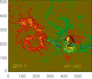
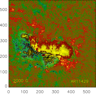
The raw magnetograms we use here were downloaded from http://jsoc.stanford.edu/jsocwiki/ReleaseNotes2, where the HMI vector magnetic field data series hmi.B_720s_e15w1332 are released for several active regions. There are two special formats, i.e., direct cutouts and remapped images. We use the remapped format which is more suitable for modeling in local Cartesian coordinates, since the images are computed with a Lambert cylindrical equal area projection centered on the tracked region. For our test, we select two active regions, AR 11283 and AR 11429, both of which produced X-class flares and thus were very non-potential. Figure fig:rawmaps shows the magnetograms for AR 11283 at 05:36 UT on 8 September 2011 and AR 11429 at 00:00 UT on 7 March 2012. The size of the magnetograms are respectively $600\times 512$ and $560\times 560$ pixels.

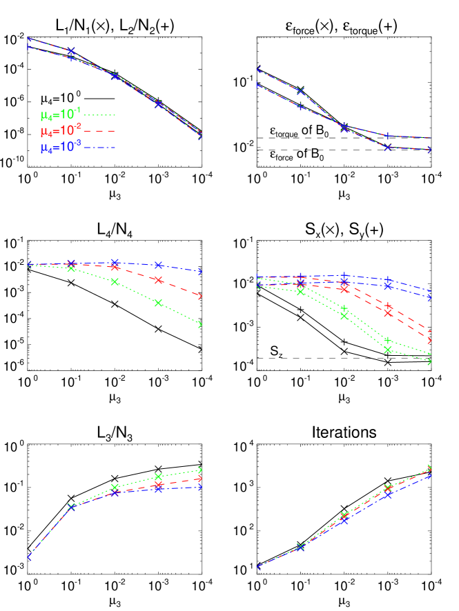
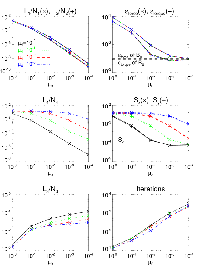
In Figures fig:result11283 and fig:result11429 we show the preprocessing results with different sets of $\mu_{3}$ and $\mu_{4}$. Since for such large magnetograms it is nontrivial to perform plenty of tests with continuous sets of weighting factors to pick the optimal one, we only compute the results for several groups of $\mu_{3}$ and $\mu_{4}$ as shown in the figures, i.e., $\mu_{3}=1,0.1,0.01,0.001,0.0001$ and $\mu_{4}=1,0.1,0.01,0.001$. For each set of weighting factors, the normalized terms $L_{l}/N_{l}$ and the smoothness and the force-free quality $\epsilon_{\rm force}$ and $\epsilon_{\rm torque}$ are plotted. By comparing the results with fixed $\mu_{3}$ but different $\mu_{4}$, we can see that the force-free parameters $L_{1}/N_{1},L_{2}/N_{2},\epsilon_{\rm force}$, and $\epsilon_{\rm torque}$ are almost entirely determined by $\mu_{3}$. When decreasing $\mu_{3}$, i.e., allowing more freedom of modifying the raw data, $L_{1}$ and $L_{2}$ decrease very quickly (their magnitude decreases quicker than that of $\mu_{3}$), but the residual force parameters $\epsilon_{\rm force}$ and $\epsilon_{\rm torque}$ reach a minimum and cannot be reduced any further. This is because the potential part ${\mathbf{B}}_{0}$ has a non-zero value of $\epsilon_{\rm force}$ and $\epsilon_{\rm torque}$ (due to numerical error of finite resolution), which is the minimum of $\epsilon_{\rm force},\epsilon_{\rm torque}$ that can be reached for the target magnetograms. The results for both tests show that $\mu_{3}=0.001$ is small enough which gives $\epsilon_{\rm force}$ and $\epsilon_{\rm torque}$ nearly the same as those of ${\mathbf{B}}_{0}$, meaning that the force in the non-potential part ${\mathbf{B}}_{1}$ is decreased near or under the level of numerical error. Even smaller $\mu_{3}$ cannot improve the quality of force-freeness, but deviates the target magnetograms farther away from the original data. Thus we set the optimal value of $\mu_{3}=0.001$. With a given value of $\mu_{3}$, the values of smoothness are controlled by $\mu_{4}$. Obviously $\mu_{4}=1$ is a good choice which gives the values of $S_{x}$ and $S_{y}$ very similar to $S_{z}$, meaning that the smoothness of the target magnetograms is consistent with their potential part ${\mathbf{B}}_{0}$. We believe the choice of weight for smoothness here is more physics-based than in other methods in which it is given more or less arbitrarily.

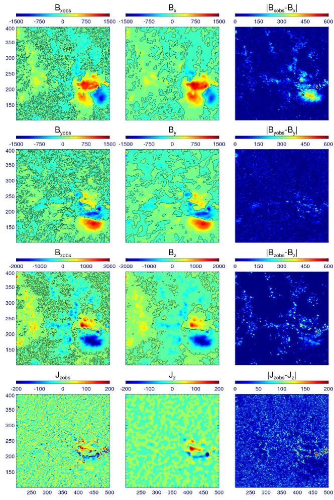
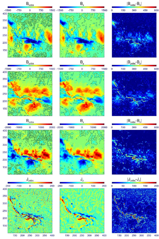
The results of preprocessing the two magnetograms with the optimal weighting factors $\mu_{3}=0.001$ and $\mu_{4}=1$ are summarized in Table tab:quality. Figures fig:map11238 and fig:map11429 show a comparison of the original and preprocessed magnetograms. Here the color-map is designed to manifest both strong and weak fields. As shown, the map after preprocessing resamples the feature of the original data while small structures tend to be smoothed out. In the bottom of the figures we plot the results for the vertical current $J_{z}$ which is calculated by taking finite differences of the transverse field

$$\ilabel{eq:alpha}J_{z}^{i,j}=\frac{B_{y}^{i+1,j}-B_{y}^{i-1,j}}{2}-\frac{B_{x}^{i,j+1}-B_{x}^{i,j-1}}{2}.$$ (26)

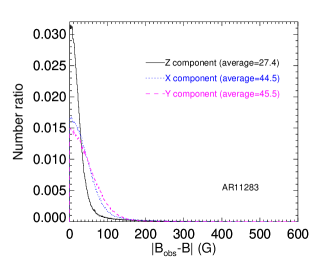
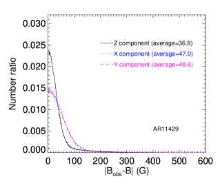
Since the numerical differences are very sensitive to noise, random noise in the data exhibits more clearly in the $J_{z}$ map, particularly in weak field regions, and they are suppressed effectively by the smoothing. Histograms are plotted in Figure fig:dBhistrogram to show the distributions of the absolute differences between the raw and preprocessed magnetograms over all the pixels. Apparently different approaches of modifying the data give different distributions, i.e., the distribution for the $z$-component is distinct from those for the $x$ and $y$-components. This is because the modification for $B_{z}$ is determined solely by the potential model, while modifications for $B_{x},B_{y}$ are additionally made by the optimization process. The change in the vertical field is less than those for the transverse field. This is consistent with the observation which measures the line-of-sight component much more precisely than the transverse field, and thus we have more freedom to modify the transverse field. Still it should be noted that here the potential-field modeled $B_{z}$ may not approximate well the real chromospheric $B_{z}$, which is preferred to be taken by direct measurements if available.

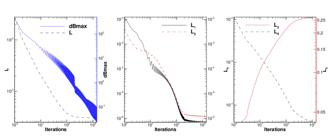
We finally show in Figure fig:iter the process of iteration in the optimization method. Only the result for AR 11283 is plotted as an example. As shown, the functional $L$ decreased very quickly. By only 200 iteration steps, it almost reaches its minimum, reduced by about two orders of magnitude from its initial value. The sub-functionals $L_{1}$ and $L_{2}$ have similar evolution, although with small oscillations, and the sub-functional $L_{4}$ keeps decreasing but very slowly after 200 steps.

5 Conclusions

sec:con

In this paper we have developed a new code of preprocessing the photospheric vector magnetograms for NLFFF extrapolation. The method is based on a simple rule that any vector magnetograms can be split into a potential field part and a non-potential part and we deal with two parts separately. Preprocessing of the potential part is simply performed by taking the data sliced at a plane about $400$ km above the photosphere from the 3D potential-field numerical solution, which is extrapolated from the observed vertical field. Then the non-potential part is modified by an optimization method to fulfill the constraints of total magnetic force-freeness and torque-freeness. As for practical computation based on numerical discretization, a strict satisfaction of force-free constraints is apparently not necessary. Also the extent of the smoothing to be applied to the data need to be carefully determined, if we want to mimic the field expansion from the photosphere to some specific height above. We use the values of force-freeness and smoothness calculated from the preprocessed potential-field part as a reference to guide the preprocessing of the non-potential field part, i.e., we require that the target magnetograms have the same level of force-freeness and smoothness as the reference data. These requirements can restrict well the values of the free parameters, i.e., the weighting factors in the optimization functional. The code is applied to the SDO/HMI data. Preprocessed results show that the method can remove efficiently the force and noise, if we properly choose the weighting factors. For two sampled HMI magnetograms, we find that the optimal weights are $\mu_{3}=0.001$ and $\mu_{4}=1$, with which the target magnetgrams can be driven to force-free and smooth with the same level as that of the numerical potential field at the bottom of the force-free domain.

The preprocessing code here is developed as a sub-program for a project of applying our extrapolation code CESE–MHD–NLFFF (Jiang, Feng, and Xiang, 2012; Jiang and Feng, 2012a) to observed data. We have applied CESE–MHD–NLFFF to SDO/HMI data with both raw and preprocessed magnetograms (Jiang and Feng, 2013). By a careful comparison of the results, we find that the quality of extrapolation is indeed improved using the preprocessed magnetograms, including the force-freeness of the results (e.g., measured by a current-weighted mean angle between the magnetic field ${\mathbf{B}}$ and electric current ${\mathbf{J}}$) and the free energy contents. For example in the extrapolation of AR 11283, the mean angle between ${\mathbf{B}}$ and ${\mathbf{J}}$ for the entire extrapolation box of $600\times 512\times 300$ pixels is reduced from $24^{\circ}$ to $17^{\circ}$ and the free energy is increased from $\approx 0.5\times 10^{32}$ erg to $1.0\times 10^{32}$ erg.

Acknowledgements

This work is jointly supported by the 973 program under grant 2012CB825601, the Chinese Academy of Sciences (KZZD-EW-01-4), the National Natural Science Foundation of China (41204126, 41274192, 41031066, and 41074122), and the Specialized Research Fund for State Key Laboratories. Data are courtesy of NASA/SDO and the HMI science teams. The authors thank the anonymous referee for invaluable comments.

References

- Aly (1989) Aly, J.J.: 1989, Sol. Phys. 120, 19.
- Amari, Boulmezaoud, and Aly (2006) Amari, T., Boulmezaoud, T.Z., Aly, J.J.: 2006, A&A 446, 691.
- Amari et al. (1997) Amari, T., Aly, J.J., Luciani, J.F., Boulmezaoud, T.Z., Mikic, Z.: 1997, Sol. Phys. 174, 129.
- Aschwanden et al. (2012) Aschwanden, M.J., Wuelser, J.P., Nitta, N.V., Lemen, J.R., DeRosa, M.L., Malanushenko, A.: 2012, ApJ 756, 124.
- Bobra, van Ballegooijen, and DeLuca (2008) Bobra, M.G., van Ballegooijen, A.A., DeLuca, E.E.: 2008, ApJ 672, 1209.
- Borrero et al. (2011) Borrero, J., Tomczyk, S., Kubo, M., Socas-Navarro, H., Schou, J., Couvidat, S., Bogart, R.: 2011, Solar Phys. 273, 267.
- DeRosa et al. (2009) DeRosa, M.L., Schrijver, C.J., Barnes, G., Leka, K.D., Lites, B.W., Aschwanden, M.J. et al.: 2009, ApJ 696, 1780.
- Fuhrmann, Seehafer, and Valori (2007) Fuhrmann, M., Seehafer, N., Valori, G.: 2007, A&A 476, 349.
- Fuhrmann et al. (2011) Fuhrmann, M., Seehafer, N., Valori, G., Wiegelmann, T.: 2011, A&A 526, A70.
- Gary (2001) Gary, G.A.: 2001, Sol. Phys. 203, 71.
- Inoue et al. (2011) Inoue, S., Kusano, K., Magara, T., Shiota, D., Yamamoto, T.T.: 2011, ApJ 738, 161.
- Jiang, Feng, and Xiang (2012) Jiang, C., Feng, X., Xiang, C.: 2012, ApJ 755, 62.
- Jiang and Feng (2012a) Jiang, C.W., Feng, X.S.: 2012, ApJ 749, 135.
- Jiang and Feng (2012b) Jiang, C.W., Feng, X.S.: 2012, Sol. Phys. 281, 621.
- Jiang and Feng (2013) Jiang, C.W., Feng, X.S.: 2013, ApJ 769, 144.
- Leka et al. (2009) Leka, K., Barnes, G., Crouch, A., Metcalf, T., Gary, G., Jing, J., Liu, Y.: 2009, Solar Phys. 260, 83.
- Liu et al. (2012) Liu, S., Su, J.T., Zhang, H.Q., Deng, Y.Y., Gao, Y., Yang, X., Mao, X.J.: 2012, ArXiv e-prints.
- McClymont, Jiao, and Mikic (1997) McClymont, A.N., Jiao, L., Mikic, Z.: 1997, Sol. Phys. 174, 191.
- Metcalf et al. (1995) Metcalf, T.R., Jiao, L., McClymont, A.N., Canfield, R.C., Uitenbroek, H.: 1995, ApJ 439, 474.
- Metcalf et al. (2008) Metcalf, T.R., DeRosa, M.L., Schrijver, C.J., Barnes, G., van Ballegooijen, A.A., Wiegelmann, T., Wheatland, M.S., Valori, G., McTtiernan, J.M.: 2008, Sol. Phys. 247, 269.
- Press et al. (1992) Press, W.H., Teukolsky, S.A., Vetterling, W.T., Flannery, B.P.: 1992, Numerical recipes in FORTRAN. The Art of Scientific Computing, Cambridge University Press, Cambridge, 414.
- Sakurai (1989) Sakurai, T.: 1989, Space Sci. Rev. 51, 11.
- Su et al. (2009) Su, Y., van Ballegooijen, A., Lites, B.W., Deluca, E.E., Golub, L., Grigis, P.C., Huang, G., Ji, H.: 2009, ApJ 691, 105.
- Tadesse (2011) Tadesse, T.: 2011, Nonlinear force-free reconstruction of the coronal magnetic field with advanced numerical methods. Ph.D. thesis, Max Planck Institute for Solar System Research.
- Turmon et al. (2010) Turmon, M., Jones, H.P., Malanushenko, O.V., Pap, J.M.: 2010, Sol. Phys. 262, 277.
- Valori, Kliem, and Fuhrmann (2007) Valori, G., Kliem, B., Fuhrmann, M.: 2007, Sol. Phys. 245, 263.
- Wheatland, Sturrock, and Roumeliotis (2000) Wheatland, M.S., Sturrock, P.A., Roumeliotis, G.: 2000, ApJ 540, 1150.
- Wiegelmann (2004) Wiegelmann, T.: 2004, Sol. Phys. 219, 87.
- Wiegelmann (2008) Wiegelmann, T.: 2008, J. Geophys. Res. 113, 3.
- Wiegelmann and Neukirch (2006) Wiegelmann, T., Neukirch, T.: 2006, A&A 457, 1053.
- Wiegelmann, Inhester, and Sakurai (2006) Wiegelmann, T., Inhester, B., Sakurai, T.: 2006, Sol. Phys. 233, 215.
- Yamamoto and Kusano (2012) Yamamoto, T.T., Kusano, K.: 2012, ApJ 752, 126.