Near-Optimal Sensor Placement
for Linear Inverse Problems

Abstract

A classic problem is the estimation of a set of parameters from measurements collected by only a few sensors. The number of sensors is often limited by physical or economical constraints and their placement is of fundamental importance to obtain accurate estimates. Unfortunately, the selection of the optimal sensor locations is intrinsically combinatorial and the available approximation algorithms are not guaranteed to generate good solutions in all cases of interest.

We propose FrameSense, a greedy algorithm for the selection of optimal sensor locations. The core cost function of the algorithm is the frame potential, a scalar property of matrices that measures the orthogonality of its rows. Notably, FrameSense is the first algorithm that is near-optimal in terms of mean square error, meaning that its solution is always guaranteed to be close to the optimal one.

Moreover, we show with an extensive set of numerical experiments that FrameSense achieves state-of-the-art performance while having the lowest computational cost, when compared to other greedy methods.

I Introduction

In many contexts, it is of interest to measure physical phenomena that vary in space and time. Common examples are temperature, sound, and pollution. Modern approaches tackling this problem are often based on wireless sensor networks (WSN), namely systems composed of many sensing nodes, each capable of measuring, processing and communicating information about the surrounding environment.

Challenges and trade-offs characterize the design of a WSN. One of the key aspects to design a successful WSN is the optimization of the spatial locations of the sensors nodes, given the location’s impact on many relevant indicators, such as coverage, energy consumption and connectivity. When the data collected by the WSN is used to solve inverse problems, the optimization of the sensor locations becomes even more critical. In fact, the location of the sensor nodes determines the error of the solution of the inverse problem and its optimization represents the difference between being able to obtain a reasonable solution or not. In this work we consider linear inverse problems defined as

$$\boldsymbol{f}={\boldsymbol{\Psi}}\boldsymbol{\alpha},$$ (1)

where $\boldsymbol{f}\in\mathbb{R}^{N}$ is the measured physical field, $\boldsymbol{\alpha}\in\mathbb{R}^{K}$ are the parameters to be estimated and ${\boldsymbol{\Psi}}\in\mathbb{R}^{N\times K}$ is the known linear model representing the relationship between the measurements and the parameters. Note that this simple model can be easily adapted to more complicated scenarios. For example, if the collected measurements are linear combinations of the physical field, as in the presence of a sampling kernel, we simply consider ${\boldsymbol{\Psi}}=\boldsymbol{\Phi}\boldsymbol{\Theta}$, where $\boldsymbol{\Phi}$ and $\boldsymbol{\Theta}$ represent the sampling kernel and the physical phenomenon, respectively.

The role of $\boldsymbol{\alpha}$ depends on the specific inverse problem. For example, if the WSN is designed for source localization, $\boldsymbol{\alpha}$ represents the location and the intensity of the field sources. On the other hand, if we are planning to interpolate the measured samples to recover the entire field, we may think of $\boldsymbol{\alpha}$ as its low-dimensional representation. In other scientific applications, for example [1, 2, 3], the solution of a linear inverse problem is a step within a complex procedure and $\boldsymbol{\alpha}$ may not have a direct interpretation. Nonetheless, the accurate estimation of $\boldsymbol{\alpha}$ is of fundamental importance.

It is generally too expensive or even impossible to sense the physical field $\boldsymbol{f}$ with $N$ sensor nodes, where $N$ is determined by the resolution of the discrete physical field. Assume we have only $L<N$ sensors, then we need to analyze how to choose the $L$ sampling locations such that the solution of the linear inverse problem (1) has the least amount of error. Namely, we would like to choose the most informative $L$ rows of ${\boldsymbol{\Psi}}$ out of the $N$ available ones. One could simply adopt a brute force approach and inspect all the possible combinations for the $L$ sensor locations. In this case, the operation count is exponential due to its combinatorial nature, making the approach unfeasible even for modest values of $N$.

It is possible to significantly reduce the computational cost by accepting a sub-optimal sensor placement produced by an approximation algorithm. In this case, near-optimal algorithms are desired since they always produce a solution of guaranteed quality. We measure this quality as the ratio between the value of the approximated solution and the value of the optimal one, and we call it the approximation factor.

I-A Problem Statement and Prior Art

We consider the linear model introduced in (1) and a WSN measuring the field at only $L<N$ locations. We denote the sets of measured locations and of available locations as $\mathcal{L}=\{i_{1},\ldots,i_{L}\}$ and $\mathcal{N}=\{1,\ldots,N\}$, respectively. Note that $\mathcal{L}\subseteq\mathcal{N}$ and $|\mathcal{L}|=L$.

The measured field is denoted as $\boldsymbol{f}_{\cal{L}}\in\mathbb{R}^{L}$, where the subscript represents the selection of the elements of $\boldsymbol{f}$ indexed by $\cal{L}$. Consequently, we define a pruned matrix ${\boldsymbol{\Psi}}_{\cal{L}}\in\mathbb{R}^{L\times K}$, where we kept only the rows of ${\boldsymbol{\Psi}}$ indexed by $\cal{L}$. We obtain a smaller linear system of equations,

$$\boldsymbol{f}_{\cal{L}}={\boldsymbol{\Psi}}_{\cal{L}}\boldsymbol{\alpha},$$ (2)

where we still recover $\boldsymbol{\alpha}$, but with a reduced set of measurements, $L\geq K$. Note that we have by definition ${\boldsymbol{\Psi}}_{\mathcal{N}}={\boldsymbol{\Psi}}$ and $\boldsymbol{f}_{\mathcal{N}}=\boldsymbol{f}$.

Given the set of measurements $\boldsymbol{f}_{\mathcal{L}}$, there may not exist an $\widehat{\boldsymbol{\alpha}}$ that solves (2). If it exists, the solution may not be unique. To overcome this problem, we usually look for the least squares solution, defined as $\widehat{\boldsymbol{\alpha}}=\arg\min_{\boldsymbol{\alpha}}\|{\boldsymbol{\Psi}}_{\cal{L}}\boldsymbol{\alpha}-\boldsymbol{f}_{\cal{L}}\|_{2}^{2}.$ Assume that ${\boldsymbol{\Psi}}_{\cal{L}}$ has rank $K$, then this solution is found using the Moore-Penrose pseudoinverse,

$$\widehat{\boldsymbol{\alpha}}={\boldsymbol{\Psi}}_{\cal{L}}^{+}\boldsymbol{f}_{\cal{L}},$$

where ${\boldsymbol{\Psi}}_{\cal{L}}^{+}=({\boldsymbol{\Psi}}_{\cal{L}}^{*}{\boldsymbol{\Psi}}_{\cal{L}})^{-1}{\boldsymbol{\Psi}}_{\cal{L}}^{*}$. The pseudoinverse generalizes the concept of inverse matrix to non-square matrices and is also known as the canonical dual frame in frame theory. For simplicity of notation, we introduce $\mathbf{T}_{\mathcal{L}}={\boldsymbol{\Psi}}_{\cal{L}}^{*}{\boldsymbol{\Psi}}_{\cal{L}}\in\mathbb{R}^{K\times K}$, a Hermitian-symmetric matrix that strongly influences the reconstruction performance. More precisely, the error of the least squares solution depends on the spectrum of $\boldsymbol{T}_{\cal{L}}$. That is, when the measurements $\boldsymbol{f}_{\cal{L}}$ are perturbed by a zero-mean i.i.d. Gaussian noise with variance $\sigma^{2}$, the mean square error ($\operatorname{MSE}$) of the least squares solution [4] is

$$\operatorname{MSE}\left(\widehat{\boldsymbol{\alpha}}\right)=\|\widehat{\boldsymbol{\alpha}}-\boldsymbol{\alpha}\|_{2}^{2}=\sigma^{2}\sum_{k=1}^{K}\frac{1}{\lambda_{k}},$$ (3)

where $\lambda_{k}$ is the $k$-th eigenvalue of the matrix $\boldsymbol{T}_{\cal{L}}$. We thus state the sensor placement problem as follows.

Problem 1.

Given a matrix ${\boldsymbol{\Psi}}\in\mathbb{R}^{N\times K}$ and a number of sensors $L$, find the sensor placement $\cal{L}$ such that

$$\arg\min_{\cal{L}}\sum_{k=1}^{K}\frac{1}{\lambda_{k}} |\mathcal{L}|=L.$$ subject to (4)

Note that if $\boldsymbol{T}_{\mathcal{L}}$ is rank deficient, that is $\operatorname{rank}(\boldsymbol{T}_{\mathcal{L}})<K$, then the $\operatorname{MSE}$ is not bounded.

A trivial choice would be to design algorithms minimizing directly the $\operatorname{MSE}$ with some approximation procedure, such as greedy ones. In practice, the $\operatorname{MSE}$ is not used because it has many unfavorable local minima. Therefore, the research effort is focused in finding tight proxies of the $\operatorname{MSE}$ that can be efficiently optimized. In what follows, we survey different approximation strategies and proxies from the literature.

I-B Prior work

Classic solutions to the sensor placement problem can be classified in three categories: convex optimization, greedy methods and heuristics.

Convex optimization methods [5, 6] are based on the relaxation of the Boolean constraints $\{0,1\}^{N}$ representing the sensor placement to the convex set $[0,1]^{N}$. This relaxation is usually not tight as heuristics are needed to choose the sensor locations and there is no a-priori guarantee on the distance from the optimal solution. The authors in [6] define an online bound for the quality of the obtained solution by looking at the gap between the primal and the dual problem.

Heuristic methods [7, 8, 9, 10, 11, 12] are valid options to reduce the cost of the exhaustive search, which has a prohibitive cost. Again, even if the methods work in practice, little can be said about the quality or the optimality of the solution.

Greedy algorithms leveraging the submodularity of the cost function [13] are a class of algorithms having polynomial complexity and guaranteed performance with regards to the chosen cost function [5, 14, 15, 16, 17]. Since the MSE is not submodular in general [15, 17], alternative cost functions have been considered [5, 14, 15, 16, 17]. The proposed methods are theoretically near-optimal with regards to the chosen cost function, but little can be said about the achieved MSE. Moreover, the local optimization of the proposed cost functions are computationally demanding, often requiring the inversion of large matrices [14]. Therefore, approximations of the cost functions have been proposed [14], offering a significant speedup for an acceptable reduction of the solution’s quality.

Beside the approximation strategy, approximation algorithms are differentiated by the chosen cost function. Under restrictive assumptions, the $\operatorname{MSE}$ can be chosen as a cost function, see [15, 18]. In [17], the authors bounded the performance of greedy algorithms optimizing $\operatorname{R}^{2}$, a measure of goodness of fit based on the $\operatorname{MSE}$, using the concept of submodularity ratio. However, such algorithm is generally less performant than the greedy algorithms optimizing proxies of the $\operatorname{MSE}$. Common proxies of the $\operatorname{MSE}$ are inspired by information theoretic measures such as entropy [12], cross-entropy [19, 16] and mutual information [14]. A popular choice is the maximization of the log determinant of $\boldsymbol{T}_{\mathcal{L}}$, being the volume of the confidence ellipsoid given by the measurements. This proxy has been historically introduced in D-Optimal experiment design [20], but has also been successfully proposed as a cost function for a convex relaxed method [6] and greedy algorithms [5]. Other proxies have also been introduced in optimal experiment design, such as maximization of the smallest eigenvalue $\lambda_{K}$ (E-Optimal design) or the maximization of the trace of $\boldsymbol{T}_{\mathcal{L}}$ (T-Optimal design). A detailed description of the different choices available for experiment design can be found in [20].

(a)

(b)

Figure 1: A graphical representation of the unit-norm rows of two matrices ${\boldsymbol{\Psi}}$ and $\boldsymbol{\Phi}$. On the left, the rows ${\boldsymbol{\Psi}}$ are optimally spread on $\mathbb{R}^{2}$ minimizing the $\operatorname{FP}$ and the $\operatorname{MSE}$. This is also know as the Mercedes-Benz frame and is a typical example of a unit-norm tight frame. On the right, ${\boldsymbol{\Psi}}$ is the frame built by adding a vector to the orthonormal basis of $\mathbb{R}^{2}$ $[\boldsymbol{\phi_{1}},\boldsymbol{\phi}_{2}]$. The three vectors are not minimizing the $\operatorname{FP}$ and therefore they are not in equilibrium with regards to the frame force. You can envision a parallel example with three electrons on a unit circle under the Coulomb force. More precisely, if the three electrons are free to move, they would reach an equilibrium when located as the vectors of ${\boldsymbol{\Psi}}$, up to a rotation factor.

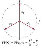
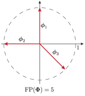
Note that there exists optimal strategies with a reasonable computational cost for some specific scenarios. This is the case when we have the freedom of completely designing the matrix ${\boldsymbol{\Psi}}_{\cal{L}}$ given the dimensions $L$ and $K$. More precisely, if $L=K$, the optimal basis corresponds to an orthonormal basis, while if $L>K$, then we are looking for a unit-norm tight frame [21, 22]. Benedetto et al. showed that each tight frame is a non-unique global minimizer of the frame potential ($\operatorname{FP}$), that is a scalar property of the frame defined as

$$\operatorname{FP}({\boldsymbol{\Psi}}_{\cal{L}})=\sum_{i,j\in\cal{L}}|\left<{\boldsymbol{\psi}}_{i},{\boldsymbol{\psi}}_{j}\right>|^{2},$$

where ${\boldsymbol{\psi}}_{i}$ is the $i$th row of ${\boldsymbol{\Psi}}_{\cal{L}}$. One of the reasons of the popularity of the $\operatorname{FP}$ in the frame theory community is its interesting physical interpretation [23]. Namely, it is the potential energy of the so-called frame force, a force between vectors inspired by the Coulomb force. The frame force and its potential energy have been introduced for their orthogonality encouraging property: the force is repulsive when the angle between the two vectors is acute, null when they are orthogonal and attractive when the angle is obtuse. A graphical explanation of this physical interpretation is given in Figure 1, where the unit-norm rows of two matrices ${\boldsymbol{\Psi}}$ and $\boldsymbol{\Phi}$ belonging to $\mathbb{R}^{3\times 2}$ are represented. While ${\boldsymbol{\Psi}}$, that is the unit-norm tight frame minimizing the $\operatorname{FP}$, has vectors as close to orthogonality as possible and therefore in equilibrium with regards to the frame force, the vectors of $\boldsymbol{\Phi}$ are not optimally close to orthogonality and the $\operatorname{FP}$ is thus not minimized. Note that according to frame theory [22], ${\boldsymbol{\Psi}}$ is the matrix that also achieves the minimum $\operatorname{MSE}$ (per component).

Note that the $\operatorname{FP}$ is also known as the total summed correlation in communication theory [24]. It is used to optimize the signatures of CDMA systems to achieve the Welch’s lower bound [25] and maximize the capacity of the channel.

Given its interpretation and its role in defining the existence of tight frames—the optimal frames in terms of $\operatorname{MSE}$—we hypothesize that the $\operatorname{FP}$ is an interesting cost function for an approximation algorithm.

I-C Our contributions

We propose FrameSense, a greedy sensor placement method that minimizes the frame potential to choose the sensing locations $\mathcal{L}$. We briefly summarize the innovative aspects of the proposed algorithm:

• Under some stability conditions regarding the spectrum of ${\boldsymbol{\Psi}}$, FrameSense is the only known algorithm, to the best of our knowledge, that is near-optimal with regards to $\operatorname{MSE}$.

• FrameSense outperforms other greedy algorithms in terms of $\operatorname{MSE}$.

• FrameSense is on par with the method based on convex relaxation [6], which uses heuristics to improve the local solution and has a significantly higher complexity.

• The computational cost of FrameSense is significantly lower with regards to the other considered algorithms.

The remainder of the paper uses the following notations: calligraphic letters as $\mathcal{C}$ indicate sets of elements, while bold letters as ${\boldsymbol{\Psi}}$ and ${\boldsymbol{\psi}}$ indicates matrices and vectors, respectively. The $k$-th largest eigenvalue of $\mathbf{T}_{\mathcal{L}}={\boldsymbol{\Psi}}^{*}_{\mathcal{L}}{\boldsymbol{\Psi}}_{\mathcal{L}}$ is denoted as $\lambda_{k}$. Moreover, we always consider a real physical field $\boldsymbol{f}$ and real matrices ${\boldsymbol{\Psi}}$ for simplicity but the extension to the complex domain does not require major adjustments.

The content is organized as follows. In Section II we introduce some frame theory concepts focusing on the role of the $\operatorname{FP}$. We describe FrameSense and the analysis of its near-optimality in Section III and we numerically compare its performance with various other algorithms in Section IV.

II The frame potential in frame theory

This section briefly introduces some of the basic concepts of frame theory that are useful to understand and analyze the proposed algorithm. Frame theory studies and designs families of matrices ${\boldsymbol{\Psi}}_{\mathcal{L}}$ such that $\boldsymbol{T}_{\mathcal{L}}$ is well-conditioned. More precisely, ${\boldsymbol{\Psi}}_{\mathcal{L}}$ is a frame for a Hilbert space $\mathbb{H}$ if there exists two scalars $A$ and $B$ such that $0<A\leq B<\infty$ so that for every $\mathbf{x}\in\mathbb{H}$ we have

$$A\|\mathbf{x}\|_{2}^{2}\leq\|{\boldsymbol{\Psi}}_{\mathcal{L}}\mathbf{x}\|_{2}^{2}\leq B\|\mathbf{x}\|_{2}^{2},$$

where $A$ and $B$ are called frame bounds. ${\boldsymbol{\Psi}}_{\mathcal{L}}$ is a tight frame when $A=B$ and its columns are orthogonal by construction. Of particular interest is the case of unit norm tight frames (UNTF); these are tight frames whose frame elements—the rows ${\boldsymbol{\psi}}_{i}$—have unit norm. These provide Parseval-like relationships, despite the non-orthogonality of the frame elements of ${\boldsymbol{\Psi}}_{\mathcal{L}}$. In addition to (3), there are other interesting relationships between the characteristics of ${\boldsymbol{\Psi}}_{\mathcal{L}}$ and the spectrum of $\boldsymbol{T}_{\mathcal{L}}$. For example, we can express the $\operatorname{FP}$ as

$$\operatorname{FP}({\boldsymbol{\Psi}}_{\mathcal{L}})=\operatorname{Trace}({\boldsymbol{T}_{\mathcal{L}}}^{*}\boldsymbol{T}_{\mathcal{L}})=\sum_{k=1}^{K}|\lambda_{k}|^{2}.$$

Moreover, the sum of the eigenvalues of $\boldsymbol{T}_{\mathcal{L}}$ is equal to the sum of the norm of the rows, $\sum_{i=1}^{L}\|{\boldsymbol{\psi}}_{i}\|^{2}=\sum_{k=1}^{K}\lambda_{k}$.

These quantities of interest take a simplified analytical form for UNTFs. In this scenario, we know [22] that the $\operatorname{FP}$ is minimum with regards to all other matrices of the same size with unit-norm rows, and it is equal to $\operatorname{FP}_{\text{UNTF}}=\frac{L^{2}}{K}$. According to [22], the optimal $\operatorname{MSE}$ is also achieved when the $\operatorname{FP}$ is minimized and it is equal to $\operatorname{MSE}_{\text{UNTF}}=\frac{K^{2}}{L}$. Note that in this case all the eigenvalues are equal, $\lambda_{\text{UNTF}}=\lambda_{i}=\frac{L}{K}\;\forall i$.

Next, we would like to intuitively explain why the $\operatorname{FP}$ is a good candidate to be a proxy for the $\operatorname{MSE}$. Consider the distance between the $\operatorname{FP}$ of a matrix with unit-norm rows ${\boldsymbol{\Psi}}_{\mathcal{L}}\in\mathbb{R}^{L\times K}$ and the $\operatorname{FP}$ of a UNTF. Then, it is possible to show that this distance is always positive and equal to

$$\operatorname{FP}({\boldsymbol{\Psi}}_{\mathcal{L}})-\operatorname{FP}_{\text{UNTF}}=\sum_{k=1}^{K}\left(\lambda_{k}-\frac{L}{K}\right)^{2},$$

where $\frac{L}{K}$ is the value of the eigenvalues $\lambda_{\text{UNTF}}$. Note that if we minimize the $\operatorname{FP}$ of ${\boldsymbol{\Psi}}_{\mathcal{L}}$, then each $\lambda_{k}$ converges to $\frac{L}{K}$.

At the same time, the distance between the $\operatorname{MSE}$ of ${\boldsymbol{\Psi}}_{\mathcal{L}}$ and the $\operatorname{MSE}$ of the UNTF can be expressed as

$$\operatorname{MSE}({\boldsymbol{\Psi}}_{\mathcal{L}})-\operatorname{MSE}_{\text{UNTF}}=\sum_{k=1}^{K}\left(\frac{1}{\lambda_{k}}-\frac{K}{L}\right).$$

Now, it is easy to see that if the eigenvalues converge to $\frac{L}{K}$, then $\operatorname{MSE}({\boldsymbol{\Psi}}_{\mathcal{L}})$ converges to the $\operatorname{MSE}$ of a UNTF, being also the optimal one [22].

III FrameSense: a near-optimal sensor placement

Even if the intuition given in Section II is clear, it does not directly explain why an algorithm placing the sensor according to the $\operatorname{FP}$ would perform well in terms of $\operatorname{MSE}$. Indeed, we need to address some complications such as matrices ${\boldsymbol{\Psi}}$ having rows with different norms and the non-uniform convergence of the eigenvalues. In what follows, we first describe the details of FrameSense and then analyze its near-optimality in terms of both the $\operatorname{FP}$ and the $\operatorname{MSE}$.

III-A The algorithm

FrameSense finds the sensor locations $\mathcal{L}$ given the known model ${\boldsymbol{\Psi}}$ and the number of available sensors nodes $L$ with a greedy minimization of the $\operatorname{FP}$. It is a greedy “worst-out” algorithm: at each iteration it removes the row of ${\boldsymbol{\Psi}}$ that maximally increases the $\operatorname{FP}$. In other words, we define a set of locations $\mathcal{S}$ that are not suitable for sensing and at each iteration we add to $\mathcal{S}$ the row that maximizes the following cost function:

$$F(\mathcal{S})=\operatorname{FP}({\boldsymbol{\Psi}})-\operatorname{FP}({\boldsymbol{\Psi}}_{\mathcal{N}\setminus\mathcal{S}}).$$ (5)

The pseudo-code for FrameSense is given in Algorithm 1.

Require: Linear Model ${\boldsymbol{\Psi}}$, Number of sensors $L$
Ensure:  Sensor locations $\cal{L}$
 

1. Initialize the set of locations, $\mathcal{L}=\emptyset$.

2. Initialize the set of available locations, ${\cal{N}}=\{1,\ldots,N\}$.

3. Find the first two rows to eliminate, $\mathcal{S}=\arg\max_{i,j\in\mathcal{N}}|\left<{\boldsymbol{\psi}}_{i},{\boldsymbol{\psi}}_{j}\right>|^{2}$.

4. Update the available locations, $\mathcal{L}=\mathcal{N}\setminus\mathcal{S}$.

5. Repeat until $L$ locations are found

   1. If $|\mathcal{S}|=N-L$, stop.

   2. Find the optimal row, $i^{*}=\arg\min_{i\in{\cal{L}}}F\left({\cal{S}}\cup i\right)$.

   3. Update the set of removed locations, $\mathcal{S}=\mathcal{S}\cup i^{*}$.

   4. Update the available locations, $\mathcal{L}=\mathcal{L}\setminus i^{*}$.

Algorithm 1 FrameSense

One may ask why we do not optimize directly the $\operatorname{MSE}$, instead of minimizing the $\operatorname{FP}$, which indirectly optimizes the $\operatorname{MSE}$. As we have already indicated, a greedy algorithm optimizing a general function, like the $\operatorname{MSE}$, converges to a local stationary point of the cost function and we have no guarantee on the distance from the global optimum. On the other hand, we can prove that FrameSense is near-optimal with regards to the $\operatorname{FP}$ by exploiting the submodularity of the cost function. In addition, we also guarantee the performance of FrameSense in terms of the $\operatorname{MSE}$, exploiting a link between $\operatorname{FP}$ and $\operatorname{MSE}$.

III-B Near-optimality of FrameSense with regards to $\operatorname{FP}$

We define the performance of FrameSense with regards to $\operatorname{FP}$ using the theory of submodular functions. We start by defining the concept of submodularity that relates to the concept of diminishing returns: if we add an element to a set $\mathcal{Y}$, the benefit is smaller or equal than adding the same element to one of the subsets of $\mathcal{Y}$. Then, we introduce a theorem by Nemhauser et al. [13] that defines the approximation factor of greedy algorithms maximizing a submodular function. We continue by showing that FrameSense satisfies the conditions of Nemhauser’s theorem and we derive its approximation factor in terms of $\operatorname{FP}$.

Definition 1 (Submodular function).

Given two sets $\mathcal{X}$ and $\mathcal{Y}$ such that $\mathcal{X}\subset\mathcal{Y}\subset\mathcal{N}$ and given an element $i\in\mathcal{N}\setminus\mathcal{Y}$, a function $G$ is submodular if it satisfies

$$G(\mathcal{X}\cup i)-G(\mathcal{X})\geq G(\mathcal{Y}\cup i)-G(\mathcal{Y}).$$ (6)

Submodular functions are useful in combinatorial optimization because greedy algorithms have favorable properties when optimizing a function with such a property. More precisely, it has been proved that the greedy maximization of submodular functions is near-optimal [13].

Theorem 1 (Near-optimal maximization of submodular function [13]).

Let $G$ be a normalized, monotone, submodular set function over a finite set $\mathcal{N}$. Let $\mathcal{L}$ be the set of $L$ elements chosen by the greedy algorithm, and let $\operatorname{OPT}=\max_{\mathcal{A}\subset\mathcal{N},|\mathcal{A}|=L}G(\mathcal{A})$ be the optimal set of elements. Then

$$G(\mathcal{L})\geq\left(1-\frac{1}{e}\right)\operatorname{G}(\operatorname{OPT}),$$

where $e$ is Euler’s number.

Namely, if $G$ satisfies the conditions of Theorem 1, then the solution of the greedy algorithm is always close to the optimal one. These conditions are satisfied by the cost function $F$ in (5), as shown in the following lemma.

Lemma 1 (Submodularity of the cost function).

The set function maximized in Algorithm 1,

$$F(\mathcal{S})=\operatorname{FP}({\boldsymbol{\Psi}})-\operatorname{FP}({\boldsymbol{\Psi}}_{\mathcal{N}\setminus\mathcal{S}}),$$ (7)

is a normalized, monotone, submodular function.

Proof.

The set function $F$ is normalized if $F(\emptyset)=0$. Here, normalization is trivially shown since ${\boldsymbol{\Psi}}={\boldsymbol{\Psi}}_{\mathcal{N}}$ by definition. To show monotonicity, we pick a generic matrix ${\boldsymbol{\Psi}}$ of $N$ rows, a set $\mathcal{X}$ and an index $i\notin\mathcal{X}$. Then, we compute the increment of $F$ due to $i$ with regards to the set $\mathcal{X}$, showing that it is always positive.

$$F(\mathcal{X}\cup i)-F(\mathcal{X}) =\operatorname{FP}({\boldsymbol{\Psi}}_{\mathcal{N}\setminus\mathcal{X}})-\operatorname{FP}({\boldsymbol{\Psi}}_{\mathcal{N}\setminus\mathcal{X}\cup{i}})$$

$$\overset{(a)}{=}\sum_{n,m\in\mathcal{A}\cup{i}}|\langle{\boldsymbol{\psi}}_{n},{\boldsymbol{\psi}}_{m}\rangle|^{2}-\sum_{n,m\in\mathcal{A}}|\langle{\boldsymbol{\psi}}_{n},{\boldsymbol{\psi}}_{m}\rangle|^{2}$$

$$=2\sum_{n\in\mathcal{A}}|\langle{\boldsymbol{\psi}}_{n},{\boldsymbol{\psi}}_{i}\rangle|^{2}+|\langle{\boldsymbol{\psi}}_{i},{\boldsymbol{\psi}}_{i}\rangle|^{2}\geq 0,$$

where $(a)$ is due to a change of variable $\mathcal{N}\setminus\mathcal{X}=\mathcal{A}$. Assuming without loss of generality that $\mathcal{Y}=\mathcal{X}\cup j$, we check the submodularity according to Definition 1 .

$$F(\mathcal{X}\cup i)-F(\mathcal{X})-F(\mathcal{Y}\cup i)+F(\mathcal{Y})$$

$$=F(\mathcal{X}\cup i)-F(\mathcal{X})-F(\mathcal{X}\cup\left\{i,j\right\})+F(\mathcal{X}\cup j)$$

$$=\operatorname{FP}({\boldsymbol{\Psi}}_{\mathcal{A}\cup\left\{i,j\right\}})-\operatorname{FP}({\boldsymbol{\Psi}}_{\mathcal{A}\cup{j}})-\operatorname{FP}({\boldsymbol{\Psi}}_{\mathcal{A}\cup{i}})+\operatorname{FP}({\boldsymbol{\Psi}}_{\mathcal{A}})$$

$$=2\sum_{n\in\mathcal{A}\cup{j}}|\langle{\boldsymbol{\psi}}_{n},{\boldsymbol{\psi}}_{i}\rangle|^{2}-2\sum_{n\in\mathcal{A}}|\langle{\boldsymbol{\psi}}_{n},{\boldsymbol{\psi}}_{i}\rangle|^{2}$$

$$=2|\langle{\boldsymbol{\psi}}_{i},{\boldsymbol{\psi}}_{j}\rangle|^{2}\geq 0.$$

∎

Now, we use Theorem 1 to derive the approximation factor of FrameSense with regards to the $\operatorname{FP}$.

Theorem 2 ($\operatorname{FP}$ approximation factor).

Consider a matrix ${\boldsymbol{\Psi}}\in\mathbb{R}^{N\times K}$ and a given number of sensors $L$, such that $K\leq L<N$. Denote the optimal set of locations as $\text{OPT}=\arg\max_{\mathcal{A}\subset\mathcal{N},|\mathcal{A}|=L}\operatorname{FP}({\boldsymbol{\Psi}}_{\mathcal{A}})$ and the greedy solution found by FrameSense as $\mathcal{L}$. Then, $\mathcal{L}$ is near-optimal with regards to the $\operatorname{FP}$,

$$\operatorname{FP}({\boldsymbol{\Psi}}_{\mathcal{L}})\leq\gamma\operatorname{FP}({\boldsymbol{\Psi}}_{\text{OPT}}),$$ (8)

where $\gamma=\left(1+\frac{1}{e}\left(\operatorname{FP}({\boldsymbol{\Psi}})\frac{K}{{{L_{\text{MIN}}}^{2}}}-1\right)\right)$ is the approximation factor and $L_{\text{MIN}}=\min_{|\mathcal{L}|=L}\sum_{i\in\mathcal{L}}\|{\boldsymbol{\psi}}_{i}\|^{2}$ is the sum of the norms of the $L$ rows with the smallest norm.

Proof:

According to Lemma 1, the cost function used in FrameSense satisfies the conditions of Theorem 1. Therefore,

$$F(\overline{\text{OPT}})-F(\mathcal{S})\leq\frac{1}{e}(F(\overline{\text{OPT}})),$$

where $F(\mathcal{S})=\operatorname{FP}({\boldsymbol{\Psi}})-\operatorname{FP}({\boldsymbol{\Psi}}_{\mathcal{N}\setminus\mathcal{S}})$ is the considered cost function, $\mathcal{S}$ is the set of rows eliminated by FrameSense and $\overline{\text{OPT}}=\mathcal{N}\setminus\text{OPT}$. If we consider the cost function, we obtain

$$\operatorname{FP}({\boldsymbol{\Psi}}_{\mathcal{N}\setminus\mathcal{S}})\leq\left(1-\frac{1}{e}\right)\operatorname{FP}({\boldsymbol{\Psi}}_{\mathcal{N}\setminus\overline{\text{OPT}}})+\frac{1}{e}\operatorname{FP}({\boldsymbol{\Psi}}).$$ (9)

Then, we note that the following minimization problem,

$$\operatorname{minimize}_{\mathcal{L}}\operatorname{FP}({\boldsymbol{\Psi}}_{\mathcal{L}}) |\mathcal{L}|=L,$$ subject to

is equivalent, under the change of variable $\mathcal{L}=\mathcal{N}\setminus\mathcal{S}$, to

$$\operatorname{minimize}_{\mathcal{S}}\operatorname{FP}({\boldsymbol{\Psi}}_{\mathcal{N}\setminus\mathcal{S}}) |\mathcal{S}|=N-L.$$ subject to

Using the equivalence in (9), we obtain

$$\operatorname{FP}({\boldsymbol{\Psi}}_{\mathcal{L}})\leq\left(1+\frac{1}{e}\left(\frac{\operatorname{FP}({\boldsymbol{\Psi}})}{\operatorname{FP}({\boldsymbol{\Psi}}_{\text{OPT}})}-1\right)\right)\operatorname{FP}({\boldsymbol{\Psi}}_{\text{OPT}}),$$

To conclude the proof, we bound from above the term $\frac{1}{e}\frac{\operatorname{FP}({\boldsymbol{\Psi}})}{\operatorname{FP}({\boldsymbol{\Psi}}_{\text{OPT}})}$. First, we consider the optimal solution OPT to select a tight frame whose rows have a summed norm of $L_{\text{OPT}}=\sum_{i\in\text{OPT}}\|{\boldsymbol{\psi}}_{i}\|^{2}$,

$$\operatorname{FP}({\boldsymbol{\Psi}}_{\mathcal{L}})\leq\left(1+\frac{1}{e}\left(\operatorname{FP}({\boldsymbol{\Psi}})\frac{K}{{L_{\text{OPT}}}^{2}}-1\right)\right)\operatorname{FP}({\boldsymbol{\Psi}}_{\text{OPT}}).$$

Then, we assume that OPT selects the rows having the smallest norm, $L_{\text{OPT}}\geq L_{\text{MIN}}=\min_{|\mathcal{L}|=L}\sum_{i\in\mathcal{L}}\|{\boldsymbol{\psi}}_{i}\|^{2}.$ ∎

Note that the $\operatorname{FP}$ of the original matrix influences significantly the final result: the lower the $\operatorname{FP}$ of ${\boldsymbol{\Psi}}$, the tighter the approximation obtained by the greedy algorithm. Therefore, FrameSense performs better when the original matrix ${\boldsymbol{\Psi}}$ is closer to a tight frame. In fact, the $\operatorname{FP}$ is bounded as follows,

$$\frac{\left(\sum_{i=1}^{N}\|{\boldsymbol{\psi}}_{i}\|^{2}\right)^{2}}{K}\leq\operatorname{FP}({\boldsymbol{\Psi}})\leq\left(\sum_{i=1}^{N}\|{\boldsymbol{\psi}}_{i}\|^{2}\right)^{2},$$

where the lower bound is reached by tight frames and the upper bound by rank 1 matrices.

Moreover, Theorem 2 suggests to remove from ${\boldsymbol{\Psi}}$ the rows whose norm is significantly smaller with regards to the others to improve the performance of FrameSense. This suggestion is intuitive, since such rows are also the least informative.

III-C Near-optimality of FrameSense with regards to $\operatorname{MSE}$

Having a near-optimal $\operatorname{FP}$ does not necessarily mean that the obtained $\operatorname{MSE}$ is also near-optimal. Here, we show that, under some assumptions on the spectrum of ${\boldsymbol{\Psi}}$, FrameSense is near-optimal with regards to the $\operatorname{MSE}.$

Before going to the technical details, we generalize the concept of number of sensors to account for the norms of the rows of ${\boldsymbol{\Psi}}$. More precisely, we keep $L$ as the number of rows and we define $L_{\mathcal{A}}=\sum_{i\in\mathcal{A}}\|{\boldsymbol{\psi}}_{i}\|^{2}$ as the sum of the norms of the rows of ${\boldsymbol{\Psi}}_{\mathcal{A}}$ for a generic set $\mathcal{A}$. We also define the two extremal values of $L_{\mathcal{A}}$,

$$L_{\text{MIN}}=\min_{\mathcal{A}\in\mathcal{N},|\mathcal{A}|=L}\sum_{i\in\mathcal{A}}\|{\boldsymbol{\psi}}_{i}\|^{2},$$ (10)

$$L_{\text{MAX}}=\max_{\mathcal{A}\in\mathcal{N},|\mathcal{A}|=L}\sum_{i\in\mathcal{A}}\|{\boldsymbol{\psi}}_{i}\|^{2},$$ (11)

indicating respectively the minimum and the maximum value of $L_{\mathcal{A}}$ among all possible selections of $L$ out of $N$ rows of ${\boldsymbol{\Psi}}$. $L_{\mathcal{A}}$ is also connected to the spectrum of $\boldsymbol{T}_{\mathcal{A}}$. Indeed, $L_{\mathcal{A}}$ is the trace of $\boldsymbol{T}_{\mathcal{A}}$ and thus it is also the sum of its eigenvalues,

$$L_{\mathcal{A}}=\sum_{i\in\mathcal{A}}\|{\boldsymbol{\psi}}_{i}\|^{2}=\operatorname{Trace}(\boldsymbol{T}_{\mathcal{A}})=\sum_{i\in\mathcal{A}}\lambda_{i}.$$

If ${\boldsymbol{\Psi}}$ has rows with unit-norm, then $L_{\mathcal{A}}=L_{\text{MIN}}=L_{\text{MAX}}=L$.

As a first step to prove the near-optimality with regards to $\operatorname{MSE}$, we consider a possible placement $\mathcal{A}$ and we bound the $\operatorname{MSE}$ of the matrix ${\boldsymbol{\Psi}}_{\mathcal{A}}$ using its $\operatorname{FP}$ and the spectrum of $\boldsymbol{T}_{\mathcal{A}}$. To obtain such a bound, we use a known inequality [26] involving variance, arithmetic mean and harmonic mean of a set of positive bounded numbers, in this case the eigenvalues of $\boldsymbol{T}_{\mathcal{A}}$. The following lemma describes the bound, while its proof is given in Appendix -A.

Lemma 2 (MSE bound).

Consider any ${\boldsymbol{\Psi}}_{\mathcal{A}}\in\mathbb{R}^{L\times K}$ with $|\mathcal{A}|=L\leq K$ and denote the spectrum of $\boldsymbol{T}_{\mathcal{A}}$ as $\lambda_{1}\geq\ldots\geq\lambda_{K}$. Then the $\operatorname{MSE}$ is bounded according to the $\operatorname{FP}$ as,

$$\operatorname{MSE}({\boldsymbol{\Psi}}_{\mathcal{A}})\leq\frac{K}{L_{\text{MIN}}}\frac{\operatorname{FP}({\boldsymbol{\Psi}}_{\mathcal{A}})}{{\lambda_{K}}^{2}},$$ (12)

$$\operatorname{MSE}({\boldsymbol{\Psi}}_{\mathcal{A}})\geq\frac{K}{L_{\text{MAX}}}\frac{\operatorname{FP}({\boldsymbol{\Psi}}_{\mathcal{A}})}{{\lambda_{1}}^{2}},$$ (13)

where $L_{\text{MIN}}$ and $L_{\text{MAX}}$ are defined as in (10) and (11).

Lemma 2 is key to study the approximation factor with regards to the $\operatorname{MSE}$. Specifically, it allows to analyze the two extremal cases:

• Given the optimal $\operatorname{FP}$, what is the lowest $\operatorname{MSE}$ we can achieve?

• Given the worst case $\operatorname{FP}$ according to Theorem 2, what is the largest $\operatorname{MSE}$ we may encounter?

Lemma 2 implies the necessity to properly bound the spectrum of any ${\boldsymbol{\Psi}}_{\mathcal{A}}$ with a given $\operatorname{FP}$ obtained from ${\boldsymbol{\Psi}}$. While it is possible to bound $\lambda_{1}$ with the $\operatorname{FP}$, it is also easy to build matrices with $\lambda_{K}=0$, compromising the bound given in (12). Therefore, we introduce the following property to control the eigenvalues of any $\boldsymbol{T}_{\mathcal{A}}$.

Definition 2 ($(\delta,L)$-bounded frame).

Consider a matrix ${\boldsymbol{\Psi}}\in\mathbb{R}^{N\times K}$ where $N\geq L$ and $N>K$. Then, we say that ${\boldsymbol{\Psi}}$ is $(\delta,L)$-bounded if, for every $\mathcal{A}\subseteq\mathcal{N}$ such that $|\mathcal{A}|=L$, $\boldsymbol{T}_{\mathcal{A}}$ has a bounded spectrum

$$\frac{L_{\text{MEAN}}}{K}-\delta\leq\lambda_{i}\leq\frac{L_{\text{MEAN}}}{K}+\delta,$$

where $1\leq i\leq K$, $\delta\geq 0$ and $L_{\text{MEAN}}=\frac{L}{N}\sum_{i\in\mathcal{N}}\|{\boldsymbol{\psi}}_{i}\|^{2}$ is average value of $L_{\mathcal{A}}$.

The concept of $(\delta,L)$-bounded frames is similar to the notion of matrices satisfying the restricted isometry property, that are used in compressive sensing to guarantee the reconstruction of a sparse vector from a limited number of linear measurements [27]. Moreover, it allows us to define an approximation factor for the $\operatorname{MSE}$ that does not depend on the $\operatorname{FP}$, the cost-function we minimize.

(a)

(b)

(c)

(d)

Figure 2: Performance comparison between FrameSense and other greedy algorithms using common cost functions. We randomly generate matrices with $N=100$ and $K=30$ and test different greedy algorithms for a varying number of placed sensors $L$. The performance is measured in terms of $\operatorname{MSE}$, so the lower the curve, the higher the performance. The shaded areas represent the positive side of the error bars, measured using the standard deviation over 100 realizations. We consider four different types of sensing matrices, and in all cases FrameSense outperforms the other algorithms. We underline the consistency of FrameSense over the four types of matrices.

Figure 3: Comparison in terms of computational time as a function of $N$ between FrameSense and other greedy algorithms using commonly considered cost functions. The lower the curve the faster the algorithm. Note how FrameSense is the fastest algorithm, the exception being the random selection. Moreover, observe how the different algorithms scales equivalently with $N$. Errors bars are not shown because they are smaller than the markers.

Theorem 3 (MSE approximation factor for $(\delta,L)$-bounded frames).

Consider a matrix ${\boldsymbol{\Psi}}\in\mathbb{R}^{N\times K}$ and $L\geq K$ sensors. Assume ${\boldsymbol{\Psi}}$ to be a $(\delta,L)$-bounded frame, let $d$ be the ratio $\left.L_{\text{MEAN}}\middle/K\right.$ and define the optimal placement in terms of $\operatorname{MSE}$ as $\text{OPT}=\arg\min_{\mathcal{A}\in\mathcal{N},|\mathcal{A}|=L}\operatorname{MSE}({\boldsymbol{\Psi}}_{\mathcal{A}})$. Then the solution $\mathcal{L}$ of FrameSense is near-optimal with regards to the $\operatorname{MSE}$,

$$\operatorname{MSE}({\boldsymbol{\Psi}}_{\mathcal{L}})\leq\eta\operatorname{MSE}({\boldsymbol{\Psi}}_{\text{OPT}})\text{ with }\eta=\gamma\frac{(d+\delta)^{2}}{(d-\delta)^{2}}\frac{L_{\text{MAX}}}{L_{\text{MIN}}},$$

where $\eta$ is the approximation factor of the $\operatorname{MSE}$ and $\gamma$ is the approximation factor of the $\operatorname{FP}$.

Proof:

First, we compute the worst case $\operatorname{MSE}$ when FrameSense yields the worst $\operatorname{FP}$, that is for $\operatorname{FP}({\boldsymbol{\Psi}}_{\mathcal{L}})=\gamma\operatorname{FP}({\boldsymbol{\Psi}}_{\text{OPT}})$. Using the upper bound (12) and the bounds on the spectrum for $(\delta,L)$-bounded frames, we have

$$\operatorname{MSE}({\boldsymbol{\Psi}}_{\mathcal{L}})\leq\frac{K}{L_{\text{MIN}}}\frac{\gamma\operatorname{FP}({\boldsymbol{\Psi}}_{\text{OPT}})}{(d-\delta)^{2}}.$$ (14)

Then, we compute the best case $\operatorname{MSE}$ when the $\operatorname{FP}$ is optimal. We note that the lower bound (13) of the $\operatorname{MSE}$ is monotonically decreasing with regards to the $\operatorname{FP}$. Therefore, we use the same strategy considered for the lower bound, and obtain

$$\operatorname{MSE}({\boldsymbol{\Psi}}_{\text{OPT}})\leq\frac{K}{L_{\text{MAX}}}\frac{\operatorname{FP}({\boldsymbol{\Psi}}_{\text{OPT}})}{(d+\delta)^{2}}.$$ (15)

Note that we consider that the optimal $\operatorname{MSE}$ is achieved for the optimal $\operatorname{FP}$ because the lower bound of the $\operatorname{MSE}$ is monotonically decreasing with regards to $\operatorname{FP}.$ Finally, we compute the $\operatorname{MSE}$ approximation ratio as the ratio between (14) and (15), obtaining the desired result. ∎

The definition of $(\delta,L)$-bounded frames is key to the proof. It turns out that many families of adequately normalized random matrices satisfy Definition 2, but it is hard to build deterministic matrices with such property. Nonetheless, FrameSense works well even for ${\boldsymbol{\Psi}}$ that are not provably $(\delta,L)$-bounded. The same happens for compressed sensing and RIP matrices [28].

III-D Practical considerations on FrameSense

One point of FrameSense that needs improvement is the optimization of the sensing energy $L_{\mathcal{L}}$. In fact, the $\operatorname{FP}$ tends to discard the rows having a larger norm, which in theory could be more relevant to minimize the $\operatorname{MSE}$. As an example, consider a matrix ${\boldsymbol{\Psi}}$ built as follows,

$${\boldsymbol{\Psi}}=\begin{bmatrix}{\boldsymbol{\Psi}}_{0}\\ C{\boldsymbol{\Psi}}_{0}\end{bmatrix},$$ (16)

where ${\boldsymbol{\Psi}}_{0}$ is a generic matrix and $C>1$ is a constant. FrameSense would sub-optimally pick rows from the first matrix, discarding the ones from the second matrix and creating a sub-optimal sensor placement. In fact, the second matrix would have a lower $\operatorname{MSE}$ thanks to the multiplicative constant $C$. To limit such phenomenon, we optimize the sensor location on ${\boldsymbol{\Psi}}^{\prime}$, that is a ${\boldsymbol{\Psi}}$ with unit-norm rows. This solution is not perfect: it removes the negative bias introduced by the norm of ${\boldsymbol{\psi}}_{i}$, but it does not exploit the sensing energy to improve the sensor placement $\mathcal{L}$. We leave to future work the study of a new $\operatorname{FP}$-based algorithm able to exploit the information contained in the norm of the rows.

We conclude this section with a quantification of the bounds given in Theorem 2 and Theorem 3 in a simple scenario. Consider a matrix ${\boldsymbol{\Psi}}\in\mathbb{C}^{N\times K}$ filled with i.i.d. Gaussian complex random variables with zero mean and variance $\sigma^{2}=1/K$. Assume that $L=c_{1}K$ and $N=c_{2}K$, with $c_{2}>1>c_{1}$. Then, we have the following inequalities verified in expectation,

$$\|{\boldsymbol{\psi}}_{i}\|_{2}=1\quad\forall i,$$

$$\frac{K}{{L_{\text{MIN}}}^{2}}=\frac{1}{{c_{1}}^{2}K},$$

$$\operatorname{FP}({\boldsymbol{\Psi}})={c_{2}}^{2}{c_{1}}^{2}K.$$

According to Theorem 2, the approximation factor of the $\operatorname{FP}$ is equal to $\gamma=1+\frac{c_{2}^{2}-1}{e}$. We assume that $K$ is sufficiently large and we consider the Marchenko-Pastur law [29] to compute the following approximated bounds for the eigenvalues of ${\boldsymbol{\Psi}}_{\mathcal{L}}$,

$$d-\delta=\sqrt{\frac{1}{c_{1}}}\left(1-\sqrt{c_{1}}\right)^{2}\leq\lambda_{i}\leq\sqrt{\frac{1}{c_{1}}}\left(1+\sqrt{c_{1}}\right)^{2}=d+\delta.$$

In this scenario, the $\operatorname{MSE}$ approximation factor is equal to,

$$\eta=\left(1+\frac{{c_{2}}^{2}-1}{e}\right)\left(\frac{1+\sqrt{c_{1}}}{1-\sqrt{c_{1}}}\right)^{4}.$$

For example, if $c_{1}=0.25$ and $c_{2}=6$, then we have $\gamma\approx 14$ and $\eta\approx 50$.

IV Numerical Results

In this section, we analyze the performance of FrameSense and compare it with state-of-the-art algorithms for sensor placement.

IV-A Synthetic data

First, we compare the $\operatorname{FP}$ with other cost functions when used in a naive greedy algorithm. Among the ones listed in Section I-B, we select the following three cost functions: mutual information [14], determinant of $\boldsymbol{T}_{\mathcal{L}}$ [5], and $\operatorname{MSE}$ [15]. We also consider an algorithm that randomly places the sensors to relate the obtained results to a random selection.

(a)

(b)

(c)

(d)

Figure 4: Tradeoff between computational time and $\operatorname{MSE}$. We randomly generate matrices—according to four different models—with $N=100$, $K=30$ and $L=50$ sensors. The performance is measured in terms of $\operatorname{MSE}$, therefore the lower the dot, the higher the performance. On the other hand, the computational time is measured in seconds. The error bars are represented as ellipsoids, where the length of the axes represent the standard deviation of the data point. Note that, FrameSense is the fastest algorithm by one order of magnitude and it is the second best algorithm in terms of $\operatorname{MSE}$. When the legend refer to a cost function, we considered a naive greedy algorithm optimizing that cost function. On the other hand, we refer to the authors for specific algorithms implementing complicated schemes and/or heuristics.

Figure 5: Analysis of the tradeoff between computational time and $\operatorname{MSE}$ for FrameSense and the convex relaxed algorithm proposed by Joshi et al. [6]. We generate 100 Gaussian matrices with $K=20$ and of increasing size $N=\{50,100,150,200,300,400,500\}$, while we place $L=0.5N$ sensors. The error bars are represented as ellipsoids, where the length of the axes represent the standard deviation of the data point. We measure the average computational time together with the average $\operatorname{MSE}$, showing that while FrameSense is significantly faster than the convex algorithm, the difference in $\operatorname{MSE}$ is minimal. Moreover, the gap in the quality of the solution decreases for an increasing size of the problem $N$.

The greedy algorithms are tested on different types of sensing matrices ${\boldsymbol{\Psi}}$:

• random matrices with Gaussian i.i.d. entries,

• random matrices with Gaussian i.i.d. entries whose rows are normalized,

• random matrices with Gaussian i.i.d. entries with ortho-normalized columns, that we call random tight frame due to the Naimark theorem [30],

• random matrices with Bernoulli i.i.d entries.

Note that the use of random matrices is sub-optimal, since we would rarely encounter such a case in a real-world scenario. However, it is the only available dataset that allows us to test thoroughly the different algorithms.

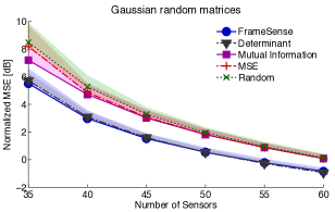
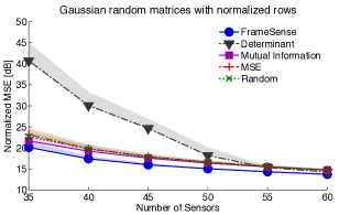
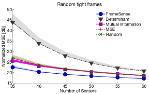
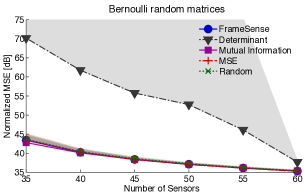
We consider ${\boldsymbol{\Psi}}\in\mathbb{R}^{100\times 30}$ and evaluate the performance in terms of $\operatorname{MSE}$ for $L=\{35,35,40,45,50,55,60\}$. We use 100 different instances for each combination, and we compute the average $\operatorname{MSE}$ as a function of $L$. Note that the $\operatorname{MSE}$ is always computed using (3), which assumes i.i.d. Gaussian noise perturbing the measurements $\boldsymbol{f}$ and a uniform distribution on $\boldsymbol{\alpha}$. The relatively small size of ${\boldsymbol{\Psi}}$ and the low number of trials are due to the lack of scalability of certain cost functions, which require the computation of large matrices. The results are given in Figure 2. We note that FrameSense is consistently outperforming all other cost functions. In the random Gaussian matrices case, the determinant shows similar results. However, looking at the Bernoulli matrices case, we see that the determinant leads to a significantly worse $\operatorname{MSE}$. Note that certain cost functions show worse performance than a random selection of the rows. While this phenomena could be partially explained by the special properties of certain families of random matrices, it indicates the importance of choosing a well-studied cost function for which we can obtain performance bounds with respect to the $\operatorname{MSE}$.

According to the theory of random matrices, any selection of rows should have the same spectrum on expectation. Therefore, it should not be possible to outperform the random selection of rows. However, the theoretical analysis of random matrices is generally valid only asymptotically, while here we show results for relatively small matrices. This phenomenon could also be of interest for other domains, such as compressed sensing, indicating the possibility of optimizing the spectrum of random matrices to improve their performance.

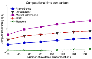
In Figure 3, we show the average computational time with regards to the number of possible sensor locations $N=\{20,50,80,\ldots,200\}$. We consider 100 random Gaussian matrices ${\boldsymbol{\Psi}}\in\mathbb{R}^{N\times 10}$ and we place $0.5N$ sensors. We underline that FrameSense is significantly faster than any other greedy algorithm, the only exception being the random selection that has a computational time close to zero. Note that the other parameters, such as as $L$ and $K$, have little influence on the computational time, which strongly depends on $N$.

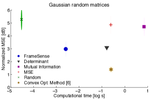
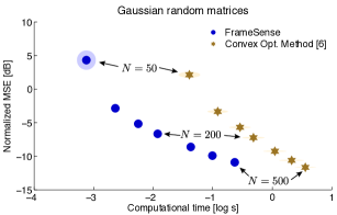
In a second experiment, we compare FrameSense with a state-of-the-art method based on convex optimization [6]. Since the algorithm proposed by Joshi et al. [6] is structurally different from FrameSense, we focus this analysis on two parameters: the computational time and the $\operatorname{MSE}$. We fix $K=20$ and the ratio between the number of sensors and the number of available locations as $L/N=0.5$. Then, we vary the number of possible locations as $N=\{50,100,150,200,300,400,500\}$. The results for Gaussian random matrices are given in Figure 5. First, we note that the convex method achieves a lower $\operatorname{MSE}$, however the performance gap decreases when we increase the number of sensors. This is not surprising, since FrameSense is a greedy algorithm that does not require parameter fine-tuning nor heuristics, while the convex relaxation method integrates some efficient heuristics. For example, at every iteration, it refines the selection by looking at all the possible swaps between the chosen locations and the discarded ones. This strategy is particularly effective when $L\approx K$: in fact, swapping just one row can improve significantly the spectrum of $\boldsymbol{T}_{\mathcal{L}}$, and consequently the $\operatorname{MSE}$ achieved by ${\boldsymbol{\Psi}}_{\mathcal{L}}$. The heuristics, while effective in terms of $\operatorname{MSE}$, increase also the computational cost. In fact, FrameSense is significantly faster.

The last comparison also opens an interesting direction for future work. In fact, the convex relaxed algorithm optimizes the determinant of $\boldsymbol{T}_{\mathcal{L}}$ and its near-optimality in terms of $\operatorname{MSE}$ has not been shown. Moreover, this cost function has been proven to be less effective compared to $\operatorname{FP}$ when used in a greedy algorithm (see Figure 2). Therefore, we expect that a convex relaxed scheme based on the $\operatorname{FP}$ has the potential to define a new state of the art, mixing the advantages of $\operatorname{FP}$ and the heuristics proposed in [6].

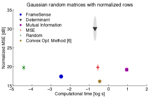
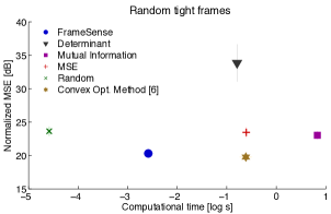
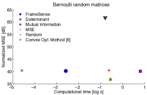
To conclude the performance analysis, we study the trade-off between computational complexity and performance for all the considered algorithms, greedy and not. We picked 100 instances of each of the random matrices proposed in the first experiment with $N=100$, $L=40$ and $K=30$. We measured the average computational time and average $\operatorname{MSE}$ obtained by each algorithm and the results are given in Figure 4. We note a general trend connecting the four subfigures: FrameSense is the fastest algorithm, by at least an order of magnitude, while its performance is just second, as previously shown, to the convex relaxed method proposed by Joshi et al. [6].

Since the sensor placement is an off-line procedure, we may argue that the computational time is of secondary importance. While this is true in many applications, there are certain applications where it is necessary to recompute $\mathcal{L}$ regularly. This is usually the case when ${\boldsymbol{\Psi}}$ changes in time due to changes of the physical field and it is possible to adaptively reallocate the sensors. In other applications, such as the ones where we attempt to interpolate the entire field from $L$ measurements, the number of possible locations $N$ grows with the desired resolution. In this case, a lower computational time is of critical importance.

(a)

(b)

Figure 6: Comparison between FrameSense, the other greedy algorithms and a coherence-based greedy algorithm proposed in [31]. In this experiment, we consider the sensors placement to estimate the temperature of an 8-core microprocessor using a limited number of sensors. Two different matrices are proposed: on the left, the matrix $\Psi\in\mathbb{R}^{420\times 16}$ is generated from a principal component analysis of known thermal maps as in [31]; on the right, the matrix $\Psi\in\mathbb{R}^{420\times 16}$ is the subsampled DCT matrix proposed in [32]. The shaded area represents the positive side of the error bar for the random sensor placement, measured using the standard deviation over 100 realizations. Note that FrameSense significantly outperforms the previous coherence-based method and the other greedy algorithms, in particular when the number of sensors is close to the number of estimated parameters, that is $K=16$.

IV-B Temperature estimation on many-core processors

We now analyze the impact of FrameSense on a real-world problem where sensor placement is of fundamental importance. We describe the problem, followed up by a simulation showing the improvement with respect to the state of the art.

The continuous evolution of process technology increases the performance of processors by including more cores memories and complex interconnection fabrics on a single chip. Unfortunately, a higher density of components increases the power densities and amplifies the concerns for thermal issues. In particular, it is key to design many-core processors that prevent hot spots and large on-chip temperature gradients, as both conditions severely affect the overall system’s characteristics. A non-exhaustive list of problems induced by thermal stress includes higher failure rate, reduced performance, increased power consumption due to current leakage and increased cooling costs. To overcome these issues, the latest designs include the thermal information into the workload allocation strategy to obtain optimal performance while avoiding critical thermal scenarios. Consequently, a few sensors are deployed on the chip to collect thermal data. However, their number is limited by area/power constraints and their optimal placement, that detects all the worst-case thermal scenarios, is still unresolved and has received significant attention [33, 8, 32, 34, 35].

An improved sensor placement algorithm would lead to a reduction of the sensing cost in terms of used silicon surface. Moreover, it implies a reduction of the reconstruction error, making possible the use of more aggressive scheduling strategies and consequently improves the processor performance. In [31], we proposed the following strategy: learn ${\boldsymbol{\Psi}}$ using a principal component analysis on an extensive set of simulated thermal maps, then place the sensors with a greedy algorithm minimizing the coherence between the rows. This work achieved a significant improvement compared to the previous state-of-the-art approach [32] that was based on specific knowledge of the spectrum of the thermal maps.

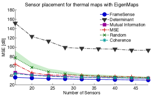
We consider a sensing matrix ${\boldsymbol{\Psi}}$ equivalent to one defined in [31] but at a lower resolution for computational reasons. More precisely, we consider thermal maps at a resolution of $16\times 15$ and a matrix ${\boldsymbol{\Psi}}\in\{420\times 16\}$. Then, we compare FrameSense, our previous greedy algorithm from [31] and the other algorithms considered in Figure 2. The results are shown in Figure 6. We note that the performance of the placement algorithm has been further improved by FrameSense, without increasing the computational cost or changing the reconstruction strategy. Moreover, we are now able to guarantee the near-optimality of the algorithm with respect to the $\operatorname{MSE}$ of the estimated thermal map.

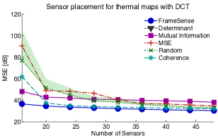
Note that we are only discussing the impact of an optimized sensor placement when we consider the ${\boldsymbol{\Psi}}$ based on the Eigenmaps described in [31]. The joint problem of sensor placement and reconstruction of thermal maps is more complex and other factors may play a fundamental role. For example, it may be more convenient to use an opportunely constructed DCT frame [32] to reduce the memory occupation at the price of a reduced reconstruction precision. The comparison of the reconstruction performance in terms of $\operatorname{MSE}$ for the various algorithms when considering the ${\boldsymbol{\Psi}}\in\mathbb{R}^{420\times 16}$ based on the DCT frame are given in Figure 6. Again, FrameSense outperforms all the other placement algorithms, in particular when the number of sensors is limited.

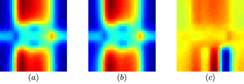
In Figure 7, we present an example of a thermal map and the two reconstructions obtained by sensor placements optimized by either FrameSense or the coherence-based algorithm. Notably, the reconstruction obtained with the sensor placement proposed by FrameSense is significantly more precise.

V Conclusions

We studied the optimization of sensor placement when the collected measurements are used to solve a linear inverse problem. The problem is equivalent to choosing $L$ rows out of $N$ from a matrix ${\boldsymbol{\Psi}}$ such that the resulting matrix has favorable spectral properties. The problem is intrinsically combinatorial and approximation algorithms are necessary for real-world scenarios. While many algorithms have been proposed, none has guaranteed performance in terms of the $\operatorname{MSE}$ of the solution of the inverse problem, which is the key merit figure.

We proposed FrameSense, a greedy worst-out algorithm minimizing the $\operatorname{FP}$. Even if this chosen cost function is well-known in frame theory for its fundamental role in the construction of frames with optimal $\operatorname{MSE}$, FrameSense is the first algorithm exploiting it as a cost function for the sensor placement problem. Our theoretical analysis demonstrates the following innovative aspects:

• FrameSense is near-optimal with respect to the $\operatorname{FP}$, meaning that it always places the sensors such that the obtained $\operatorname{FP}$ is guaranteed to be close to the optimal one.

• under RIP-like assumptions for ${\boldsymbol{\Psi}}$, FrameSense is also near-optimal with respect to the $\operatorname{MSE}$. Note that FrameSense is the first algorithm with this important property.

Figure 7: Examples of reconstruction of a thermal map of resolution $56\times 60$ using two different sensor placements. The real thermal map is depicted in $(a)$, while the reconstructed thermal maps using FrameSense and the algorithm proposed in [31] are given in $(b)$ and $(c)$, respectively. $L=16$ sensors are placed to measure $K=16$ parameters and the measurements are corrupted by noise with an SNR of 8.5 dB. Note that the reconstruction using FrameSense is close to the real map, while the other one is extremely noisy. The details regarding the generation of the thermal maps are available in [31].

We provided extensive numerical experiments showing that FrameSense achieves the best performance in terms of $\operatorname{MSE}$ while having the lowest computational complexity when compared to many other greedy algorithms. FrameSense is also competitive performance-wise with a state-of-the-art algorithm based on a convex relaxation proposed in [6], while having a substantially smaller computational time.

We showed that FrameSense has appealing performance on a real-world scenario, the reconstruction of thermal maps of many-core processors. We showed a potential for reducing the number of sensors required to estimate precisely the thermal distribution on a chip, reducing the occupied area and the consumed power by the sensors.

Future work will be three-fold. First, it is foreseeable to relax the RIP-like condition on ${\boldsymbol{\Psi}}$ by considering that the characteristics of the $\operatorname{FP}$ are potentially sufficient to avoid ${\boldsymbol{\Psi}}_{\mathcal{L}}$ matrices with an unfavorable spectral distribution. Moreover, it would be interesting to show that there exists matrices, random or deterministic, that are $(\delta,L)$-bounded frames. Second, we believe that a convex relaxed scheme based on the $\operatorname{FP}$ integrating the heuristics proposed by Joshi et al. [6] could improve significantly the $\operatorname{MSE}$ of the obtained solution, while keeping the near-optimality thanks to the $\operatorname{FP}$. Third, we would like to derive a new cost function that exploits the sensing energy of the rows, as described in Section III-D.

-A Proof of Lemma 2

In this section, we bound the $\operatorname{MSE}$ of a matrix ${\boldsymbol{\Psi}}_{\mathcal{A}}\in\mathbb{R}^{L\times K}$ as a function of its $\operatorname{FP}$ and the spectrum $\left\{\lambda_{i}\right\}_{i=1}^{K}$ of $\boldsymbol{T}_{\mathcal{L}}$.

First, consider the harmonic mean $\operatorname{H}=\frac{K}{\sum_{k}\frac{1}{\lambda_{j}}}$, the arithmetic mean $\operatorname{A}=\frac{\sum_{k}\lambda_{k}}{K}$ and the standard deviation $\operatorname{S}=\sqrt{\frac{1}{K}\sum_{k}\left(\lambda_{k}-A\right)^{2}}$ of the eigenvalues of $\boldsymbol{T}_{\mathcal{L}}$. All these quantities are linked to $\operatorname{MSE}\left({\boldsymbol{\Psi}}_{\mathcal{A}}\right)$,the number of sensors $L$ and $\operatorname{FP}\left({\boldsymbol{\Psi}}_{\mathcal{A}}\right)$. More precisely, we have

$$\operatorname{H}=\frac{K}{\operatorname{MSE}\left({\boldsymbol{\Psi}}_{\mathcal{A}}\right)},$$

$$\operatorname{A}=\frac{L_{\mathcal{A}}}{K},$$

$$\operatorname{S}=\sqrt{\frac{1}{K}\left(\operatorname{FP}\left({\boldsymbol{\Psi}}_{\mathcal{A}}\right)-\frac{{L_{\mathcal{A}}}^{2}}{K}\right)}.$$

Then, we consider the following bounds for the harmonic mean of a set of positive numbers derived by Sharma [26],

$$\frac{(M-\operatorname{S})^{2}}{M(M-2\operatorname{S})}\leq\frac{\operatorname{A}}{\operatorname{H}}\leq\frac{(m+\operatorname{S})^{2}}{m(m+2\operatorname{S})},$$

where $m$ and $M$ are the smallest and the largest number in the set. We use the expressions of $\operatorname{A}$ and $\operatorname{H}$ and we remove the mixed term in the denominator to obtain,

$$\frac{K^{2}}{L_{\mathcal{A}}}\left(1+\frac{\operatorname{S}^{2}}{M^{2}}\right)\leq\operatorname{MSE}\left({\boldsymbol{\Psi}}_{\mathcal{A}}\right)\leq\frac{K^{2}}{L_{\mathcal{A}}}\left(1+\frac{\operatorname{S}^{2}}{m^{2}}\right).$$

As expected when the $\operatorname{FP}$ achieves its global minima, that is $\operatorname{S}=0$, we achieve the optimal MSE of a tight frame.

To conclude the proof, we consider the two bounds separately starting from the lower one. Let $M=\lambda_{1}$ and we plug in the value of $S$. We also consider without loss of generality $L_{\mathcal{A}}\leq L_{\text{MAX}}$, since we can always improve the $\operatorname{MSE}$ by increasing the sensing power $L_{\mathcal{A}}$. Then,

$$\operatorname{MSE}\left({\boldsymbol{\Psi}}_{\mathcal{L}}\right)\geq\frac{K^{2}}{L_{\text{MAX}}}\left(1+\frac{\operatorname{FP}({\boldsymbol{\Psi}}_{\mathcal{A}})}{K{\lambda_{1}}^{2}}-\frac{{L_{\text{MAX}}}^{2}}{K^{2}{\lambda_{1}}^{2}}\right).$$

We obtain the final result by using lower bound on the largest eigenvalue: $\lambda_{1}\geq\frac{L_{\text{MAX}}}{K}$.

The approach to prove the upper bound is exactly symmetrical. Specifically, consider $m=\lambda_{N}$, $L_{\mathcal{A}}\geq L_{\text{MIN}}$ and use the upper bound on the smallest eigenvalue $\lambda_{N}\leq\frac{L_{\text{MAX}}}{K}$.

References

- [1] M. Vetterli, P. Marziliano, and T. Blu, “Sampling signals with finite rate of innovation,” IEEE Trans. Signal Process., vol. 50, no. 6, pp. 1417–1428, 2002.
- [2] R. G. Baraniuk and M. B. Wakin, “Random projections of smooth manifolds,” Found. Comput. Math., vol. 9, no. 1, pp. 51–77, 2009.
- [3] A. M. Bruckstein, D. L. Donoho, and M. Elad, “From sparse solutions of systems of equations to sparse modeling of signals and images,” SIAM Review, vol. 51, no. 1, pp. 34–81, 2009.
- [4] M. Fickus, D. G. Mixon, and M. J. Poteet, “Frame completions for optimally robust reconstruction,” arXiv, July 2011.
- [5] M. Shamaiah, S. Banerjee, and H. Vikalo, “Greedy sensor selection: Leveraging submodularity,” in IEEE Conference on Decision and Control (CDC), 2010.
- [6] S. Joshi and S. Boyd, “Sensor selection via convex optimization,” IEEE Trans. Signal Process., vol. 57, no. 2, pp. 451–462, 2009.
- [7] M. Al-Obaidy, A. Ayesh, and A. F. Sheta, “Optimizing the communication distance of an ad hoc wireless sensor networks by genetic algorithms,” Artif. Intell. Rev., vol. 29, no. 3-4, 2008.
- [8] R. Mukherjee and S. Memik, “Systematic temperature sensor allocation and placement for microprocessors,” in Design Automation Conference (DAC), 2006.
- [9] S. Lau, R. Eichardt, L. Di Rienzo, and J. Haueisen, “Tabu search optimization of magnetic sensor systems for magnetocardiography,” IEEE Trans. Magn., vol. 44, no. 6, pp. 1442–1445, 2008.
- [10] P. L. Chiu and F. Y. S. Lin, “A simulated annealing algorithm to support the sensor placement for target location,” in Canadian Conference on Electrical and Computer Engineering, 2004.
- [11] D. J. C. MacKay, “Information-based objective functions for active data selection,” Neural Comput., vol. 4, no. 4, pp. 590–604, 1992.
- [12] H. Wang, K. Yao, G. Pottie, and D. Estrin, “Entropy-based sensor selection heuristic for target localization,” in International Conference on Information Processing in Sensor Networks (IPSN), 2004.
- [13] G. Nemhauser, L. Wolsey, and M. Fisher, “An analysis of approximations for maximizing submodular set functions—I,” Math. Prog., vol. 14, pp. 265–294, 1978.
- [14] A. Krause, A. Singh, and C. Guestrin, “Near-optimal sensor placements in Gaussian processes: Theory, efficient algorithms and empirical studies,” J. Mach. Learn. Res., vol. 9, pp. 235–284, 2008.
- [15] A. Das and D. Kempe, “Algorithms for subset selection in linear regression,” in ACM Symposium on Theory of Computing (STOC), 2009.
- [16] M. Naeem, S. Xue, and D. C. Lee, “Cross-Entropy optimization for sensor selection problems,” in International Symposium on Communications and Information Technologies (ISCIT), 2009.
- [17] A. Das and D. Kempe, “Submodular meets spectral: greedy algorithms for subset selection, sparse approximation and dictionary selection,” in International Conference on Machine Learning (ICML), 2011.
- [18] D. Golovin, M. Faulkner, and A. Krause, “Online distributed sensor selection,” in International Conference on Information Processing in Sensor Networks (IPSN), 2010.
- [19] N. Ramakrishnan, C. Bailey-Kellogg, S. Tadepalli, and V. N. Pandey, “Gaussian processes for active data mining of spatial aggregates,” in International Conference on Data Mining (SDM), 2005.
- [20] D. M. Steinberg and W. G. Hunter, “Experimental design: review and comment,” Technometrics, vol. 26, no. 2, pp. 71–97, 1984.
- [21] V. K. Goyal, M. Vetterli, and N. Thao, “Quantized overcomplete expansions in IRn: Analysis, synthesis, and algorithms,” IEEE Trans. Inf. Theory, vol. 44, no. 1, pp. 16–31, 1998.
- [22] J. Benedetto and M. Fickus, “Finite normalized tight frames,” Adv. Comput. Math., vol. 18, no. 2, pp. 357–385, 2003.
- [23] P. G. Casazza, M. Fickus, J. Kovačević, M. Leon, and J. Tremain, “A physical interpretation of tight frames,” in Harmonic analysis and applications, pp. 51–76. Springer, 2006.
- [24] M. Rupf and J. L. Massey, “Optimum sequence multisets for synchronous code-division multiple-access channels,” IEEE Trans. Inf. Theory, vol. 40, no. 4, pp. 1261–1266, 1994.
- [25] J. Kovacevic and A. Chebira, “Life beyond bases: The advent of frames (Part II),” IEEE Signal Process. Mag., vol. 24, no. 5, pp. 115–125, 2007.
- [26] R. Sharma, “Some more inequalities for arithmetic mean, harmonic mean and variance,” J. Math. Inequal, vol. 2, pp. 109–114, 2008.
- [27] E. J. Candès and M. B. Wakin, “An introduction to compressive sampling,” IEEE Signal Process. Mag., vol. 25, no. 2, pp. 21–30, 2008.
- [28] H. Monajemi, S. Jafarpour, M. Gavish, D. L. Donoho, S. Ambikasaran, S. Bacallado, D. Bharadia, Y. Chen, Y. Choi, and M. Chowdhury, “Deterministic matrices matching the compressed sensing phase transitions of Gaussian random matrices,” Proc. Natl. Acad. Sci. U.S.A., vol. 110, no. 4, pp. 1181–1186, 2013.
- [29] R. Couillet and M. Debbah, “Signal processing in large systems: a new paradigm,” IEEE Signal Process. Mag., vol. 30, no. 1, pp. 24–39, 2013.
- [30] J. Kovačević and A. Chebira, “Life beyond Bases: The advent of frames (Part I),” IEEE Signal Process. Mag., vol. 24, no. 4, pp. 86–104, 2007.
- [31] J. Ranieri, A. Vincenzi, A. Chebira, D. Atienza, and M. Vetterli, “EigenMaps: algorithms for optimal thermal maps extraction and sensor placement on multicore processors,” in Design Automation Conference (DAC), 2012.
- [32] A. N. Nowroz, R. Cochran, and S. Reda, “Thermal monitoring of real processors: techniques for sensor allocation and full characterization.,” in Design Automation Conference (DAC), 2010.
- [33] R. Cochran and S. Reda, “Spectral techniques for high-resolution thermal characterization with limited sensor data,” in Design Automation Conference (DAC), 2009.
- [34] S. Reda, R. Cochran, and A. N. Nowroz, “Improved thermal tracking for processors using hard and soft sensor allocation techniques,” IEEE Trans. Comput., vol. 60, no. 6, pp. 841–851, 2011.
- [35] S. Sharifi and T. Š. Rosing, “Accurate direct and indirect on-chip temperature sensing for efficient dynamic thermal management,” IEEE Trans. Comput.-Aided Des. Integr. Circuits Syst., vol. 29, no. 10, pp. 1586–1599, 2010.