Two-dimensional SIR epidemics with long range infection
Abstract
We extend a recent study of susceptible-infected-removed epidemic processes with long range infection (referred to as I in the following) from 1-dimensional lattices to lattices in two dimensions. As in I we use hashing to simulate very large lattices for which finite size effects can be neglected, in spite of the assumed power law for the probability that a site can infect another site a distance vector apart. As in I we present detailed results for the critical case, for the supercritical case with , and for the supercritical case with . For the latter we verify the stretched exponential growth of the infected cluster with time predicted by M. Biskup. For we find generic power laws with dependent exponents in the supercritical phase, but no Kosterlitz-Thouless (KT) like critical point as in 1-d. Instead of diverging exponentially with the distance from the critical point, the correlation length increases with an inverse power, as in an ordinary critical point. Finally we study the dependence of the critical exponents on in the regime , and compare with field theoretic predictions. In particular we discuss in detail whether the critical behavior for slightly less than 2 is in the short range universality class, as conjectured recently by F. Linder et al.. As in I we also consider a modified version of the model where only some of the contacts are long range, the others being between nearest neighbors. If the number of the latter reaches the percolation threshold, the critical behavior is changed but the supercritical behavior stays qualitatively the same.
I Introduction
Epidemic spreading processes have attracted increasing attention in the statistical physics community Newman (2002). In the simplest case of short range infection, no cooperative effects Janssen et al. (2004); Bizhani et al. (2012), and ‘removal’ after the infection (i.e. either immunization or death), this ‘general epidemic process’ Mollison (1977); Grassberger (1983) generates ordinary percolation clusters. In the present paper we shall deal with the generalization to the case where the process lives on a 2-d square lattice and at least some of the infections have long range. More precisely we shall study cases where each site can infect a finite number of other sites, and the probability for an infection to ‘jump’ a distance vector decreases for large as with .
Models of this type were first suggested by Mollison (1977). A first calculation of critical exponents in Grassberger (1986) was flawed, as pointed out by Janssen Janssen et al. (1999), and numerical verifications of the exponents calculated in Janssen et al. (1999) where presented in Linder et al. (2008).
These works were done in the spirit of the renormalization group (RG) for critical phenomena, and have to be seen in the context of other models with long range interactions, most prominently the Ising model Fisher et al. (1972); Sak (1973); Yamazaki (1977); Gusmão and Theumann (1983); Honkonen and Nalimov (1989); Luijten and Messingfeld (2001); Luijten and Blöte (2002). As we shall discuss later in detail, they give most unambiguous results for , where analytic results can be obtained by means of perturbative field theoretic RG.
Related to this was work on the case , which started already very early with papers by Ruelle Ruelle (1969), Dyson Dyson (1969), Anderson Anderson et al. (1970), Thouless Thouless (1969) and others. The main result obtained there was that the 1-dimensional Ising model with not only has a phase transition, but that the critical point is of Kosterlitz-Thouless (KT) type: Below the critical temperature one finds power laws with continuously varying exponents, while near the critical point the correlation length increases exponentially with the inverse distance from it. The most detailed numerical verification of the Ising model predictions is in Luijten and Messingfeld (2001). Analogous mathematical results for the Potts model and for percolation were obtained in Cardy (1981); Schulman (1983); Aizenman and Newman (1986); Aizenman et al. (1988), but where not tested numerically for more than two decades, because of the obvious problem of simulating the very large lattices required to overcome finite size effects. They were verified only recently in Grassberger (2013) (denoted as I in the following), where hashing was used to simulate 1-d lattices of size .
Independently of the above mentioned work on SIR epidemics with long range contacts leading to power laws, increasingly much interest has been devoted recently to supercritical epidemics with . Partly this comes from the interest in the navigability of small world networks Kleinberg (2000), partly from interest in the spreading of various agents (viruses like influenza or HIV, computer viruses, rumors, and even money Brockmann et al. (2006); Brockmann and Hufnagel (2007)) on real world networks. But even apart from such epidemic-like processes, spatial networks with long range links have become powerful paradigms for complex real world systems Barthélemy (2011). Supercritical SIR epidemics with long range infection provide the easiest and most straightforward way to generate them.
The main objective of the present paper is to extend the simulations of I to two spatial dimensions. Again we shall use hashing, in order to simulate square lattices with sites. We could have easily increased this to sites with only minor loss of efficiency, but we checked that finite size effects can be safely neglected already with sites, for nearly all values of (except for very close and below zero) and for all observables. While these simulations have no finite lattice size corrections, there are of course finite cluster size corrections, or eqivalently corrections to scaling due to the finite duration of the epidemic. We thus complement these simulations also with simulations on finite lattices (up to ) where we followed all epidemics until they died. In Sec. 2 we shall define the models in detail, and sketch the main results. Supercritical epidemics with will be discussed in Sec. 3, while the case is treated in Sec. 4. Finally, the critical case is studied in Sec. 5, and our conclusions are drawn in Sec. 6.
II The model and basic features
We shall only deal with basic SIR epidemics on the square lattice with periodic boundary conditions. In all simulations the lattice size is sites, time is discrete and the infective period is one time step, after which sites become immune. We start always with a single infected site at , all other sites being susceptible. In each time step every infected site tries to infect in average other sites. If these sites are no longer susceptible, no replacements for them are chosen, i.e. the number of new infections is just reduced.
As in I, we consider two different models as how the target sites for new infections are selected. Most of the simulations were done for model (A), where each target site with distance vector from the infectious site is chosen randomly with probability . More precisely, we select first such sites, and then one more site is chosen with probability .
In model (B) (studied only in Sec. IV) we first infect each of the four neighbors with probability , and then choose additional targets as in model (A). For this means that the process is always supercritical, and for it implies that every epidemic always leads to an infinite cluster. We include this model for comparison with results in the mathematical literature Biskup (2004); Benjamini and Berger (2001); Berger (2004); Coppersmith et al. (2002), where the emphasis was on supercritical long range percolation.
Following Linder et al. Linder et al. (2008), we define for implicitly
by the following simple algorithm:
(i) We first chose two random numbers uniformly from .
(ii) If , we discard them and choose a new pair until .
(iii) Finally, we define
where all four sign combinations are chosen with equal probability. (iv) When computing the position of the new infected site, we added x and used periodic boundary conditions.
For this can be modified suitably, but we shall not give any details as we will in the following show only simulations for . These simulations took in total about four CPU years on modern PCs.
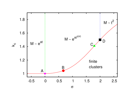
The phase diagram for model (A) is shown in Fig. 1. Below the continuous curve, i.e. for small values of , there are only finite clusters with probability 1. Infinite epidemics can exist only above this critical curve . For clusters are tree-like, i.e. the probability that a given site is one a finite loop decreases as an inverse power of the lattice size . This implies in particular for (for slightly larger than 0, we found numerically that the critical curve scales as ). The masses of supercritical clusters with (i.e., to the left of the left dashed line) increase thus exponentially with time. In contrast, for (to the right of the the right hand dashed line) supercritical clusters are essentially compact with linearly increasing size, i.e. their masses increase . In between, for , the masses of supercritical clusters increase as stretched exponentials with dependent exponents, as proven in Biskup (2004, 2009). In general, for dimensions of space, the boundaries between mean field, intermediate range and short range are at and Biskup (2004, 2009).
For critical epidemics, however, the boundaries between these mean field, intermediate, and short range regimes are different. Critical exponents are mean field like for all ( for spatial dimensions), i.e. to the left of point B Janssen et al. (1999); Linder et al. (2008). For all critical exponents depend continuously on , until the short range regime is reached. According to Linder et al. (2008), this happens at point C which corresponds to ( in general), where and are the order parameter and correlation length critical exponents for ordinary (short-range) percolation). Our own simulations, presented in Sec. 5, suggest that the short range regime extends only down to . The detailed critical behavior for is unclear.
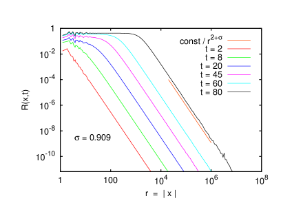
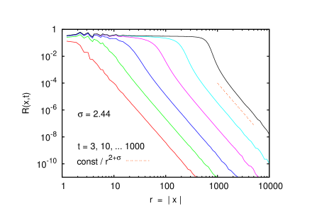
At and also the spatial structure of clusters of removed sites changes qualitatively. Assume that the epidemic started at . Then the density of removed sites decreases for any asymptotically as
| (1) |
for all , while becomes increasingly flat when . The latter is illustrated for in Fig. 1 of I, while the former is illustrated in Fig. 2.
Eq. (1) holds also for when , but at smaller distances the density decays faster than a power law, see Fig. 3. At least for supercritical epidemics this transition between the behaviors illustrated in Figs. 2 and 3 happens exactly at . Whether this is still true for critical epidemics will be discussed in Sec. 5.
III Supercritical Behavior for .
Although most studies of percolation and epidemic processes in the physics literature deal only with critical cases, it is clear that supercritical processes are of utmost practical importance. Indeed, it can be argued that most real epidemics like rabies, HIV, or various strands of influenza are far supercritical, take place in two dimensions of space, and are transmitted – due to long distance travels – by effective contacts with long range. Accordingly, there are several papers in the recent physics literature where either the spreading or the topology of the generated clusters were studied.
Typical examples for the former are Mancinelli et al. (2002); del Castillo-Negrete et al. (2003) and Brockmann and Hufnagel (2007), where front propagation was studied by mean field type arguments. While a finite speed of propagation was claimed in Brockmann and Hufnagel (2007), velocities that increase exponentially with time were found in Mancinelli et al. (2002); del Castillo-Negrete et al. (2003). As regards the topology of the cluster of removed sites, the main discussion was whether it forms a small world network (with graph diameter increasing logarithmically with the number of sites), has dimension two (as for short range epidemics), or is in between Sen and Chakrabarti (2001); Sen et al. (2001); Moukarzel and Argollo de Menzes (2002); Goswami et al. (2011); Emmerich et al. (2012).
As seen from Fig. 2, the spatial structure of cluster is rather simple. For small distances from the seed, there is a region of constant density smaller than 1, while there is a power law decay at larger densities. Indeed, Fig. 2 and similar plots for other values of are compatible, for large , with a scaling form
| (2) |
with
| (3) |
and a smooth cross-over between the two regimes. The fact that for all can be shown easily. Indeed, since the chance for site to get infected by site is , the probability for it to have never been infected is
| (4) |
giving
| (5) |
According to Eq. 2, the function also controls the geometric average radial size,
| (6) |
It also controls the size of the cluster of infected sites at any given time, which is a fuzzy ring of radius .
If the size would increase exponentially with time, as obtained in mean field theory Mancinelli et al. (2002); del Castillo-Negrete et al. (2003), this would mean that the cluster has the small world property, since its graph diameter is . On the other hand, if the radius would increase linearly Brockmann and Hufnagel (2007), its dimension would be . Actually, as proven rigorously in Biskup (2004, 2009), neither is correct. Instead, the size increases for any dimension like a stretched exponential,
| (7) |
with
| (8) |
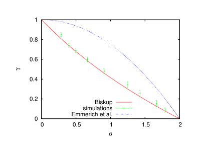
For one has , i.e. one obtains the small world behavior of mean field theory. For , on the other hand, . Qualitatively similar behavior was suggested in Emmerich et al. (2012) on the basis of numerical simulations, but the detailed functional form of obtained in Emmerich et al. (2012) was different.
-
•
First of all, for finite slightly different results are obtained when , the number of active sites, or the number of removed (‘immune’) sites is considered, although they all should show the same asymptotic behavior up to powers of . In the following we shall concentrate on .
-
•
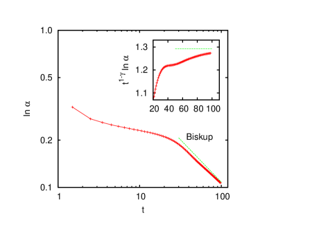
Secondly, as found also in I, directly fitting with a stretched exponential gives much too large estimates for . It is much better to define an effective growth rate
(9) which should, according to Eq. (7), decrease as .
-
•
For small values of , does increase exponentially with for very long times, if is not very large. The reason is that the deviation from exponential increase is due to saturation effects, and these set in very late for small and . This is clearly seen in Fig. 4, where is plotted against on a log-log plot. The straight dashed line is the prediction of Eqs. (7) and (8), and it gives a decent fit only for . Due to this effect, we were not able to verify Eq. (8) for .
-
•
As seen in the insert in Fig. 4, even for large values of there are strong systematic deviations from the predicted asymptotic behavior (notice that statistical errors in Fig. 4 are much smaller that the line width). Similar systematic corrections were also found for all other values of and . It seems that they were underestimated in I and are responsible for most of the systematic overestimation of found in that paper.
IV The case
In the supercritical phase, the transition between intermediate and short-range behaviors happens at . For we found in I that the number of infected sites increases for with a power law
| (10) |
provided was larger than a critical value . The power depended continuously on , and the behavior near the critical point was of Kosterlitz-Thouless type with the correlation length (and time) increasing like a stretched exponent with the distance from criticality. The order parameter (the density of the infinite cluster) was a constant at criticality, showing that the transition is first order.
Indeed, except for details this behavior for had been predicted long ago, and some aspects had even been proven rigorously Cardy (1981); Schulman (1983); Aizenman and Newman (1986); Aizenman et al. (1988). Comparably detailed predictions are not available for . It was conjectured in Benjamini and Berger (2001) that scaling with continuously varying exponents as in Eq. (10) holds for model (B) with (i.e., when every site is connected to each of its neighbors, so that ), but neither the dependence of on nor the behavior in model (A) are known.
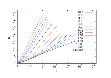
Values of for model (A) and for different values of are shown in Fig. 6. We see that indeed all curves for show power laws for large , with exponents decreasing with . As approaches from above, this asymptotic power law sets in later and later. At the same time, in this limit a different power law is observed for small , with an exponent which is compatible within errors with the exponent for critical SIR epidemics with short range contacts Grassberger (1992) (a more detailed comparison with short range SIR epidemics will be given in the next section).
For model (B) with the behavior is slightly different. In that case the process is always supercritical, and thus the asymptotic power laws hold down to . There is no time regime for small where the asymptotic power law is replaced by a different power law. This is not true for model (B) with . Although the process is also in this case supercritical for any number of long range contacts (and thus the threshold value of is also trivial), we found that otherwise the behavior is similar to the one shown in Fig. 6: When converges from above towards the critical value , converges to a value that is larger than the value for short range critical SIR epidemics. Indeed this value seems to be compatible with the limit found for model (A), i.e.
| (11) |
for both model (A) and model (B) with .
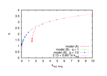
The exponents are plotted against in Fig. 7, together with analogous exponents for model (B). For large one sees a logarithmic increase similar to the one found in one spatial dimension,
| (12) |
Indeed, this behavior is common to both models, because short range bonds (which make the entire difference between models (A) and (B) are irrelevant when .
.
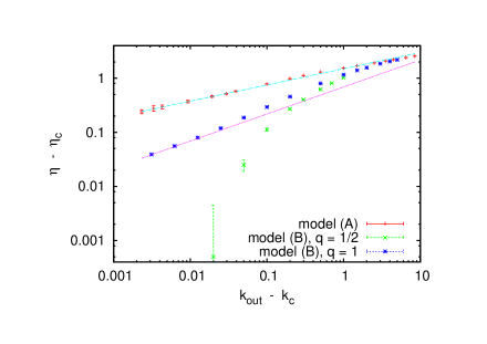
The detailed threshold behavior of cannot be seen from Fig. 7, therefore we show in Fig. 8 the same data plotted on a log-log plot, where we also changed the abscissa from to and the vertical axis from to . We see clear indications for power laws in model (A) and in model (B) with , while the data suggest a different behavior for model (B) with . More precisely, the data for model (B) with suggest
| (13) |
while for model (A) we find .
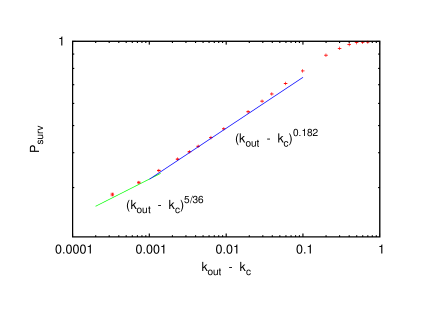
For , the percolation transition at is known to be discontinuous Aizenman and Newman (1986); Aizenman et al. (1988), as found also numerically in I. This is not the case for , as seen from Fig. 9. There we see that the survival probability vanishes at the critical point, as expected for a second order transition. Indeed, for values of very close to we see that , where is compatible with the order parameter exponent for ordinary (short range) critical percolation. This is not surprising, as we expect this scaling for all , but the huge corrections to scaling visible in Fig. 9 indicate that we should be careful with any quick conclusion. The detailed behavior at the critical point will be discussed in the next section.
V Critical Behavior
V.1 “Easy” regions and general overview
First we shall discuss the “easy” regions, i.e. values of far from the transition points B, C and D in Fig. 1, while the vicinities of these points will be discussed in later subsections.
For one is far in the mean field regime. We do not show any data, but it suffices to say that all critical exponents agreed with with their predictions to very high accuracy. There was also no problem near point A in Fig. 1, where the supercritical model changes from mean field to the intermediate phase. We expect of course highly non-trivial behavior as one goes from the critical line into the supercritical phase, when (see I for the analogous situation in ), but this seems to leave no traces on the critical line. Similarly, there is no problem for , where we recover short range behavior.
For intermediate values we do not have exact predictions for the critical exponents, but in the central part of this region, say , we find rather clean scaling laws with only moderate corrections to scaling. Typical results obtained for , e.g., are shown in Figs. 10 to 15.
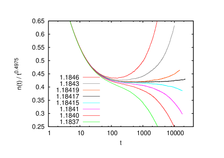
In Fig. 10 we show the average number of infected sites as a function of for various values of near the critical point. More precisely, in order to do justice to the very small error bars, we plotted , where is an estimate for the critical exponent. If it is chosen correctly, the data for should be horizontal for large . We see of course considerable corrections for , but they do not prevent precise estimates of and .
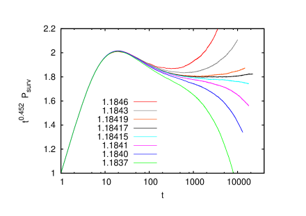
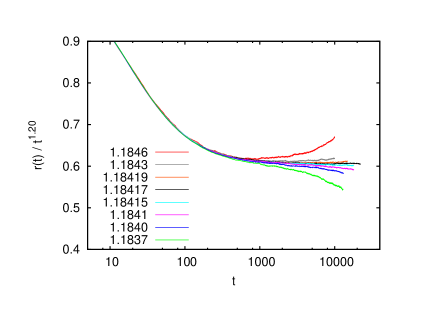
Similar plots for the survival probability and for the (geometric) average radius of the cluster of infected sites are shown in Figs. 11 and 12. They show that power laws
| (14) |
are indeed observed for the same value of . Also they satisfy the hyperscaling relation .
While and are sufficient to describe scaling exactly at the critical point, one more exponent is needed to describe scaling near the critical point. For this we can use e.g. the order parameter exponent or the correlation length exponent . For our growth simulations, the most convenient exponent is, however, which describes how the correlation time diverges as . It also describes how fast the different curves in Figs. 10 to 12 diverge at . Technically it is defined by defining first , and using then the finite-time scaling ansatz
| (15) |
where is an everywhere analytic universal scaling function.
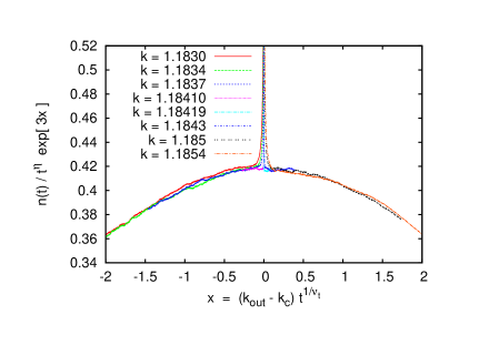
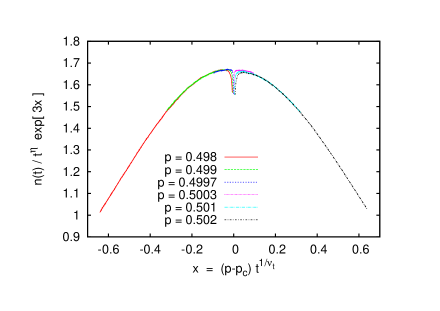
The most precise way to measure it in ordinary percolation is to relate to correlations between cluster sizes and cluster perimeter lengths Lorenz and Ziff (1998); Grassberger (2003, 2006). In the present case this cannot be used, so we had to estimate it from data collapse plots, although these are notoriously unreliable in the presence of strong corrections to scaling. Results for are shown in Fig. 13, and analogous results for ordinary bond percolation are shown for comparison in Fig. 14. In order to improve the accuracy, we plotted in both cases not against , but we multiplied the former by a suitable exponential , where the constant is chosen such as to make the scaling function horizontal at .
We see a good data collapse both in Fig. 13 and in Fig. 14, with obvious deviations near due to scaling violations at small (in Fig. 14 we only plotted data for ). For bond percolation we used of course the exactly known values for and the estimates of the critical exponents from Grassberger (1992), while we used in Fig. 13 the parameters determined from Fig. 10. We obtained .
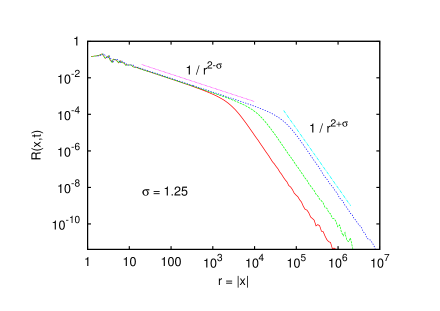
Finally, let us discuss the densities of removed sites, i.e. the densities of the percolation cluster at different times (the densities of active sites are trivially related). In Fig. 15 we see two different power laws (as also found in I for the 1-d case). More precisely, we find the same scaling law Eq. (2), but with
| (16) |
Again can be taken equal to , the geometric average cluster radius. As in the 1-d case this gives immediately a relation between the critical exponents Janssen et al. (1999),
| (17) |
(notice that was defined differently in I, as , while we now use the more conventional definition ). This is satisfied within statistical errors.
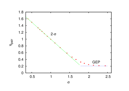
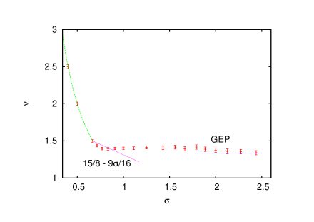
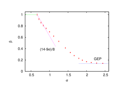
In general, we define the pair connectedness exponent by
| (18) |
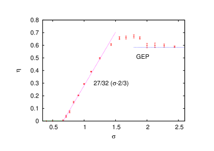
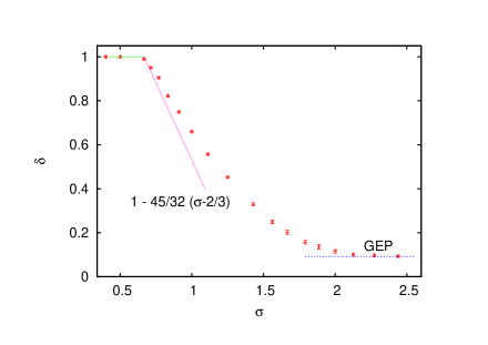
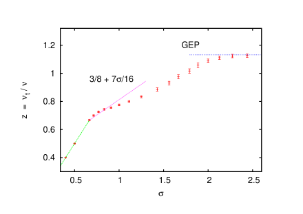
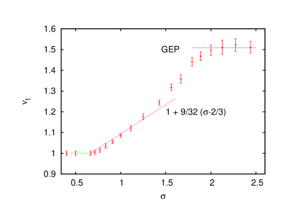
for . We also obtain the correlation length exponent by . Using these, we summarize our numerical results for the critical exponents in Figs. 16 to 22. In these plots we also indicate the results for ordinary percolation (the “General Epidemic Process, GEP) and for mean percolation, and the -expansion results of Janssen et al. (1999). While these results need no further comment in the “easy” regions, the results in the “hard” regions will be discussed in the following subsections. Here we just point out that all exponents are very precisely given by the mean field values for . For there are much larger corrections to the (presumably exact) GEP values, hinting at considerable finite-time corrections. We should say that the error bars in the “hard” regions are dominated by uncertainties in the extrapolation . They are not straightforward statistical errors, and their estimation is highly subjective, as for all critical exponents. It is quite obvious that some error bars (e.g. those for ) are wrong, but we included them on purpose, stressing thereby that meaningful error bars are virtually impossible. As we said, details are given in the following subsections.
In the intermediate region, different exponents follow the predictions of the -expansion to varying degree. Overall, the agreement is best for , while it is worst for .
V.2 The critical case for
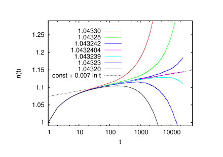
As we said, we encountered no problems for . Results exactly at are shown in Fig. 23. We see that indeed at the critical point, with very small but clearly visible corrections. These corrections are compatible with being logarithmic,
| (19) |
but the smallness of the amplitude suggests that they are more likely to be log-log corrections,
| (20) |
with . Precise fits of this form are if course meaningless, unless they were guided by theory.
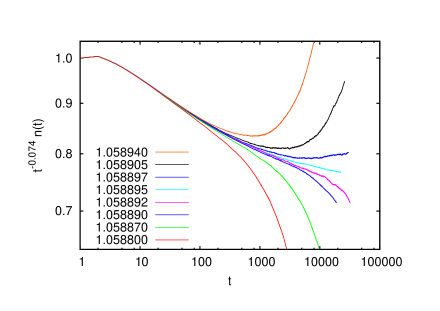
The situation is much worse for slightly larger than 2/3, as also seen from Figs. 16 to 22. In Fig. 24 we show for . None of the curves in this plot is linear, showing that the scaling limit is not yet reached even for . Curves for finally turn upward, showing that is larger than this value. If we assume conservatively that the curve for becomes asymptotically horizontal, then the value used in this plot is the correct exponent. But it is smaller than the value 0.087 predicted by the -expansion, indicating that corrections to scaling are even larger than suggested by Fig. 24. Similar problems were seen also for and 0.833, and had been found also in I for .
V.3 The intermediate to short range cross-over
Even worse corrections to scaling were found at the cross-over from intermediate to short range behavior, near points C and D in Fig. 1.
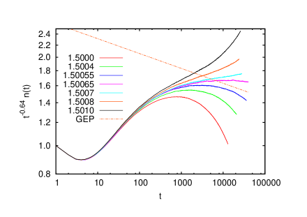
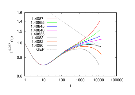
The growth of at is shown in Fig. 25. More precisely, we show there , where the power of the prefactor was chosen so that the most straight curves are roughly horizontal at large . But none of the curves is really straight. Moreover, for we expect all scaling laws to agree with short range epidemics. The scaling for the latter, corresponding to , is indicated by the dashed-dotted line. Similar plots were obtained for all . Results for
| (21) |
are e.g. shown in Fig. 26.
According to Ref. Linder et al. (2008), the ordinary (short range, GEP) percolation universality class prevails for all . The main reason for this is that
| (22) |
is supposed to be an exact result Janssen et al. (1999) in the intermediate critical phase. The latter seems indeed supported by Fig. 20, if we interpret the deviations seen there as finite time corrections. While this could be consistent with Fig. 26, it would be very hard to reconcile this conjecture with Fig. 25. If there is no singularity at , it would be very hard to understand the huge finite time corrections seen in the latter.
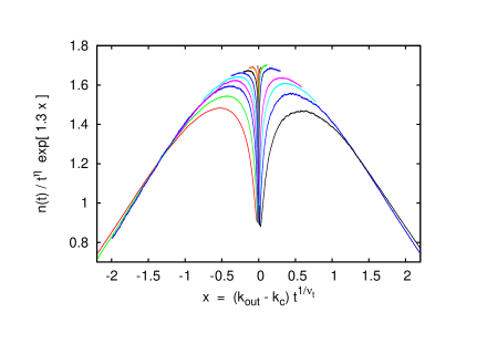
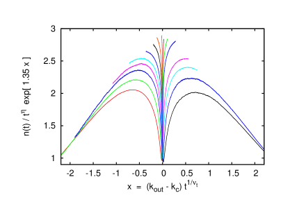
A further argument against the conjecture that ordinary GEP universality extends to comes from collapse plots similar to Figs. 13 and 14. In Fig. 27 we show twice the same data for , once using the critical exponent suggested by Fig. 25 (panel a), and then using the GEP exponents and (panel b). At first sight, it seems that panel a shows the better collapse. But we should not forget that a good collapse is only demanded for large , i.e. in the wings of the figure (, say). There, panel b shows the better collapse. But the scaling function – the envelope of the individual curves – has a parabolic shape only in panel a. In panel b it seems to be tent-like, or has an even worse cusp singularity at .
We conclude thus that the universality class does indeed change at . The critical exponents there are still those of the GEP (as suggested also by Fig. 9), but the scaling functions become singular, presumably due to logarithmic corrections to scaling.
Very puzzling is that some exponents () seem to keep their GEP values down to , while others () seem to change at . For , the situation is unclear.
It is not entirely clear why none of these problems were seen in the simulations of Linder et al. (2008). It is true that these authors used much smaller statistics (5000 runs for each parameter set, while each curve in the figures shown above is based on to runs). They also used much smaller lattices, for which finite lattice effects became a problem for large , while the above results are free of any finite lattice corrections. Still, the effects seen e.g. in Figs. 25 and 26 are hard to miss.
V.4 Finite lattice simulations at
Finally, we performed also simulations on finite lattices, in order obtain independent estimates for the fractal dimension of the percolation cluster and for exponents and . In I we had refrained from such simulations, because it was not clear how finite size effects should be described in the Kosterlitz-Thouless type transition that holds there at . For , however, the transition is a standard second order phase transition (except for possible logarithmic corrections), and we can assume that the usual finite size scaling (FSS) applies.
In the following we show only results for , since there the discrepancy between the scenarios proposed in Linder et al. (2008) and in the present paper is most clear. At face value, the simulations presented in the last subsection suggest that and ( is the fractal dimension of the cluster of “removed” sites), while according to Linder et al. (2008) these deviations should vanish in the scaling limit . In the above simulations we studied the limit for finite , while simulations on finite lattices allow us to study the limit for finite . It is hoped that both limits together can clarify the situation better than either limit by itself.
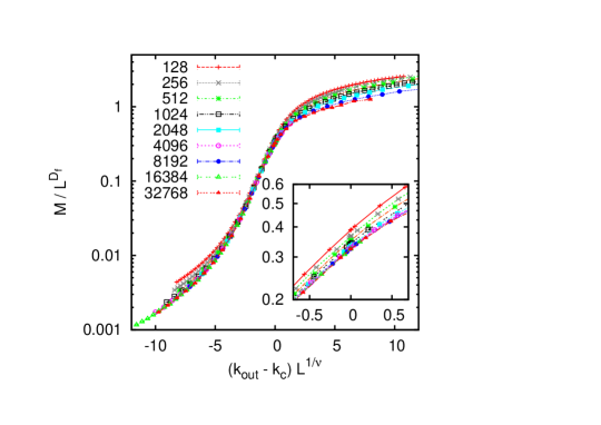
In Fig. 28 we show a data collapse based on the FSS ansatz
| (23) |
where is the mass of the cluster of “removed” (i.e. previously infected) sites. We see substantial scaling violations far away from the critical point, which was of course to be expected. The main plot of the figure suggests that these scaling violations are very small in the central (scaling) region of the plot. The insert shows that this is not quite true, but that the main violations come from small values of . The data for large suggest that
| (24) |
From these we obtain . These values are significantly different from their values for ordinary percolation, but are fully consistent with the values obtained in the last subsection.
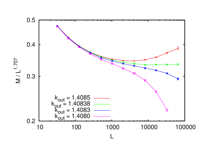
While this is a further indication that the cross-over to ordinary percolation does not happen at , it is not very convincing since scaling corrections are notoriously easy to miss in such data collapse plots. Therefore we also show in Fig. 29 log-log plots of against , for several values of close to . Asymptotically, these curves should veer up (down), if is larger (smaller) than . From Fig. 26 (and from the corresponding plot for we see two main alternatives.
-
•
Either (a): assumes the GEP value, in which case ;
-
•
Or (b): , in which case .
The data in Fig. 26 clearly indicate that the value 1.4085 is supercritical, while 1.408 and 1.4083 are subcritical, in perfect agreement with Fig. 26. But they also suggest strongly that is very close to critical. In this case the fractal dimension would be , which is definitely smaller than the value of ordinary percolation. On the basis of Fig. 26 alone, a critical value 1.40835 seems unlikely but not excluded. But it would give an even smaller value of and is thereby clearly excluded. Our final estimate is , where the uncertainty is mainly due to the uncertainty of .
VI Discussion and Conclusions
This work was triggered by recent discussions in the physics literature of spatially embedded networks with long range connections Barthélemy (2011); Sen and Chakrabarti (2001); Moukarzel and Argollo de Menzes (2002); Sen et al. (2001); Goswami et al. (2011); Kosmidis et al. (2008); Li Daqing et al. (2011); Emmerich et al. (2012) and supercritical epidemic processes leading to such networks del Castillo-Negrete et al. (2003); Mancinelli et al. (2002); Brockmann and Hufnagel (2007). Our simulations showed that most of these speculations are obsolete, but in retrospect this was to be expected. The correct topology of such networks was known rigorously since 2004 Biskup (2004). If the probability to infect a neighbor at distance decays as with , then the number of nodes reached by a path of length increased like a stretched exponential with known (and non-trivial) exponent. Our simulations fully agree with this prediction, in spite of the notorious difficulty to fit stretched exponentials.
Another class of problems is concerned with the supercritical behavior at . It was observed already in the late 1960’s that the case is special. For instance, the 1-d Ising model shows a phase transition for , while it has no transition for . For 1-d percolation, a seminal early result was that there is a discontinuous phase transition at with Kosterlitz-Thouless like behavior in the supercritical regime Aizenman and Newman (1986). No analogous result was known in two dimensions, although there are conjectures Benjamini and Berger (2001) that there also might exist continuously varying exponents in the supercritical phase. In the present paper we verify this conjecture and suggest various scaling laws related to it.
In contrast to the 1-d case, the percolation transition in the 2-d case with is continuous. Indeed, there are very strong theoretical arguments that the critical exponents at this point are exactly those of ordinary percolation or, as far as temporal aspects are concerned, of the “general epidemic process” (GEP). On the other hand, there is a long-standing debate for the Ising model (where the situation in this respect should be very similar) whether the ordinary short-range behavior should end at or extend some way into the region Fisher et al. (1972); Sak (1973); Yamazaki (1977); Gusmão and Theumann (1983); Honkonen and Nalimov (1989); Luijten and Blöte (2002). This debate is mostly centered around field theoretic arguments, but the most recent simulations Luijten and Blöte (2002) seemed to have settled the problem: The ordinary short-rang behavior extends a finite amount into the region . The same conclusion was reached for percolation in Linder et al. (2008).
Our present simulations show rather convincingly that this is wrong – at least for percolation, but the theoretical analogy suggests also for the Ising model. There is a singularity at , and at least some of the critical exponents are different for all from those for ordinary percolation. While we are rather confident about this basic claim 111Notice that one cannot use the huge corrections to scaling seen e.g. in Fig. 25 to argue away the problem. If there were no singularity at , there would be no reason for any large corrections to scaling., details are much harder to pin down due to huge corrections to scaling. This represents the main open problem related to the present paper.
The field theory that had given rise to the above debate can be treated by renormalization group methods near Janssen et al. (1999), where a field theoretic -expansion predicts anomalous critical exponents up to first order in . When comparing our simulations with these predictions, we find again large discrepancies, which might suggest that the -expansion is more singular that expected. Again more works would be needed to settle this question.
In summary, percolation with long range infection is a fascinating problem. It touches basic questions of renormalization group theory, it has applications to real-world epidemics, and it sheds light on the structure of real-world complex networks. And, finally, it still shows a number of open questions after having been studied for more than 40 years.
Acknowledgments
For very helpful discussions I want to thank Aicko Schumann and Deepak Dhar. I also want to thank the latter for the kind hospitality at the Tata Institute of Fundamental Research in Mumbai, where part of this work was done. The work was begun at the Complexity Science Group at the Universality of Calgary. Finally my thanks go to Haye Hinrichsen and Hans-Karl Janssen for illuminating correspondence.
References
- Newman (2002) M. E. J. Newman, Phys. Rev. E 66, 016128 (2002).
- Janssen et al. (2004) H.-K. Janssen, M. Müller, and O. Stenull, Phys. Rev. E 70, 026114 (2004).
- Bizhani et al. (2012) G. Bizhani, M. Paczuski, and P. Grassberger, Phys. Rev. E 86, 011128 (2012).
- Mollison (1977) D. Mollison, J. R. Stat. Soc. B 30, 283 (1977).
- Grassberger (1983) P. Grassberger, Math. Biosc. 63, 157 (1983).
- Grassberger (1986) P. Grassberger, “Spreading of epidemic processes leading to fractal structures,” in Fractals in Physics, edited by L. Pietronero and E. Tosatti (Elsevier, 1986) p. 273.
- Janssen et al. (1999) H.-K. Janssen, K. Oerding, F. van Wijland, and H. J. Hilhorst, Eur. Phys. J. B 7, 137 (1999).
- Linder et al. (2008) F. Linder, J. Tran-Gia, S. R. Dahmen, and H. Hinrichsen, J. Phys. A 41, 185005 (2008).
- Fisher et al. (1972) M. E. Fisher, S. Ma, and B. G. Nickel, Phys. Rev. Lett. 29, 917 (1972).
- Sak (1973) J. Sak, Phys. Rev. B 8, 281 (1973).
- Yamazaki (1977) Y. Yamazaki, Phys. Lett. 61A, 207 (1977).
- Gusmão and Theumann (1983) M. A. Gusmão and W. K. Theumann, Phys. Rev. B 28, 6545 (1983).
- Honkonen and Nalimov (1989) J. Honkonen and M. Y. Nalimov, J. Phys. A 22, 751 (1989).
- Luijten and Messingfeld (2001) E. Luijten and H. Messingfeld, Phys. Rev. Lett. 86, 5305 (2001).
- Luijten and Blöte (2002) E. Luijten and W. J. Blöte, Phys. Rev. Lett. 89, 025703 (2002).
- Ruelle (1969) D. Ruelle, Statistical Mechanics: Rigorous Results (Benjamin, 1969).
- Dyson (1969) F. J. Dyson, Commun. Math. Phys. 91, 212 (1969).
- Anderson et al. (1970) P. W. Anderson, G. Yuval, and D. R. Hamann, Phys. Rev. B 1, 4464 (1970).
- Thouless (1969) D. J. Thouless, Phys. Rev. 187, 732 (1969).
- Cardy (1981) J. Cardy, J. Phys. A 14, 1407 (1981).
- Schulman (1983) L. S. Schulman, J. Phys. A 16, L639 (1983).
- Aizenman and Newman (1986) M. Aizenman and C. M. Newman, Commun. Math. Phys. 107, 611 (1986).
- Aizenman et al. (1988) M. Aizenman, J. T. Chayes, L. Chayes, and C. M. Newman, J. Stat. Phys. 50, 1 (1988).
- Grassberger (2013) P. Grassberger, J. Stat. Mech. (2013).
- Kleinberg (2000) J. Kleinberg, in Proceedings of the thirty-second annual ACM symposium on Theory of computing, STOC ’00 (ACM, New York, NY, USA, 2000) pp. 163–170.
- Brockmann et al. (2006) D. Brockmann, L. Hufnagel, and T. Geisel, Nature 439, 462 (2006).
- Brockmann and Hufnagel (2007) D. Brockmann and L. Hufnagel, Phys. Rev. Lett. 98, 178301 (2007).
- Barthélemy (2011) M. Barthélemy, Physics Reports 499, 1 (2011).
- Biskup (2004) M. Biskup, Ann. Prob. 19, 2938 (2004).
- Benjamini and Berger (2001) I. Benjamini and N. Berger, Rand. Struct. Alg. 19, 102 (2001).
- Berger (2004) N. Berger, (2004), arXiv:math:0409021 .
- Coppersmith et al. (2002) D. Coppersmith, D. Gamarnik, and M. Sviridenko, Rand. Struct. Alg. 21, 1 (2002).
- Biskup (2009) M. Biskup, (2009), arXiv:math:0406379v2 .
- Mancinelli et al. (2002) R. Mancinelli, D. Vergni, and A. Vulpiani, Europhys. Lett. 60, 532 (2002).
- del Castillo-Negrete et al. (2003) D. del Castillo-Negrete, B. A. Carreras, and V. E. Lynch, Phys. Rev. Lett. 91, 018302 (2003).
- Sen and Chakrabarti (2001) P. Sen and B. Chakrabarti, J. Phys. A 34, 7749 (2001).
- Sen et al. (2001) P. Sen, K. Banerjee, and T. Biswas, Phys. Rev. E 66, 037102 (2001).
- Moukarzel and Argollo de Menzes (2002) C. F. Moukarzel and M. Argollo de Menzes, Phys. Rev. E 65, 056709 (2002).
- Goswami et al. (2011) S. Goswami, S. Biswas, and P. Sen, Physica A 390, 972 (2011).
- Emmerich et al. (2012) T. Emmerich, A. Bunde, S. Havlin, Li Guanlian, and Li Daqing, (2012), arXiv:1206.5710 .
- Grassberger (1992) P. Grassberger, J. Phys. A: Math. Gen. 25, 5475 (1992).
- Lorenz and Ziff (1998) C. D. Lorenz and R. M. Ziff, Phys. Rev. E 57, 230 (1998).
- Grassberger (2003) P. Grassberger, Phys. Rev. E 67, 036101 (2003).
- Grassberger (2006) P. Grassberger, J. Stat. Mech. 2006, P01004 (2006).
- Kosmidis et al. (2008) K. Kosmidis, S. Havlin, and A. Bunde, Europhys. Lett. 82, 48005 (2008).
- Li Daqing et al. (2011) Li Daqing, K. Kosmidis, A. Bunde, and S. Havlin, Nature Physics 7, 481 (2011).
- Note (1) Notice that one cannot use the huge corrections to scaling seen e.g. in Fig. 25 to argue away the problem. If there were no singularity at , there would be no reason for any large corrections to scaling.