Non-Standard Models, Solar Neutrinos, and Large $\theta_{13}$

Abstract

Solar neutrino experiments have yet to see directly the transition region between matter-enhanced and vacuum oscillations. The transition region is particularly sensitive to models of non-standard neutrino interactions and propagation. We examine several such non-standard models, which predict a lower-energy transition region and a flatter survival probability for the ⁸B solar neutrinos than the standard large-mixing angle (LMA) model. We find that while some of the non-standard models provide a better fit to the solar neutrino data set, the large measured value of $\theta_{13}$ and the size of the experimental uncertainties lead to a low statistical significance for these fits. We have also examined whether simple changes to the solar density profile can lead to a flatter ⁸B survival probability than the LMA prediction, but find that this is not the case for reasonable changes. We conclude that the data in this critical region is still too poor to determine whether any of these models, or LMA, is the best description of the data.

I Introduction

With the recent precision measurements of $\theta_{13}$ Ahn et al. (2012); An et al. (2013), the model of neutrino mixing is nearly complete. Of the seven new parameters added to the standard model to describe neutrino flavor transformation, only two remain unmeasured: the sign of the mass difference between the first and third mass eigenstates, and the value of the CP-violating phase $\delta$. For a large fraction of neutrino transformation phenomenology, however, the current knowledge of the parameters is expected to be good enough to describe neutrino measurements very accurately. Much of the trust in the model comes from the fact that it neatly mirrors quark mixing, which has been subject to intense scrutiny for over four decades. Yet the model of neutrino mixing is still just that—a model—and until we test that model with the kind of precision with which we have explored the rest of particle physics, we do not know whether it is in fact a complete description of neutrinos.

Construction of a broad precision measurement program with neutrino oscillations suffers not only because of the difficulty in detecting neutrinos, but also because the model makes few predictions other than oscillations themselves. In vacuum, experiments can measure oscillation behavior very precisely, but any deviation seen between predicted transformation probability and observation must first be interpreted as a change to the mixing parameters, rather than new physics. A search for new physics thus relies primarily on looking for deviations from the $L/E$ behavior that mass-difference-driven oscillations must have. Such searches can be sensitive to interesting new physics scenarios such as transformation to sterile neutrinos Aguilar et al. (2001); Aguilar-Arevalo et al. (2010); Adamson et al. (2011), or neutrino decay Gninenko (2009); Barger et al. (1999).

The situation is dramatically different once neutrino passage through matter is considered. The weakness of neutrino interactions allows coherent processes - including those from new interactions or more exotic physics - to affect flavor transformation in a measurable way. Indeed, even in Wolfenstein’s Wolfenstein (1978) seminal paper, he considers primarily the effects of flavor-changing neutral currents (FCNC) as a driver of neutrino flavor transformation in matter. Mikheyev and Smirnov Mikheyev and Smirnov (1986) subsequently demonstrated that ‘standard’ oscillations in matter of varying density—such as that of the Sun—can lead to resonant flavor conversion. This implied that even tiny effects may be observable. MSW flavor transformation is an explicit prediction of the Standard Model and the model of neutrino oscillations. It states that given measured mixing parameters, which can be provided independently from solar neutrino measurements, and density profiles of the Sun and the Earth, the phenomenology of the MSW effect is exactly specified. Yet any interaction with matter that distinguishes neutrino states, even interactions weaker than the weak interaction itself, can spoil the agreement with MSW predictions. That precision measurements using solar neutrinos are possible has been demonstrated very clearly by the observed hints of non-zero $\theta_{13}$ that came out of comparing solar neutrino measurements with those of the KamLAND reactor experiment Aharmim et al. (2010). The precision of this comparison rivaled that of the measurements by the dedicated Double CHOOZ Abe et al. (2012) experiment.

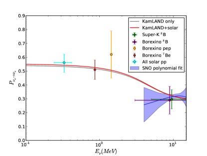
While many future experiments Akiri et al. (2011); Kisiel et al. (2009); Abe et al. (2011a) are planned to terrestrially observe matter-enhanced oscillations, and thus look for non-standard effects, to date the only large observed matter enhancement is for solar neutrinos. In Fig. 1 we show the predictions of the survival probability for solar neutrinos, spanning the energy regime from the lowest-energy $pp$ neutrinos to the highest-energy $hep$ neutrinos. We show both a curve using just the mixing parameters as measured by KamLAND Gando et al. (2011) and one with all solar data included, using the best-fit large-mixing angle (LMA) parameters. As has been pointed out by many authors Bahcall and Peña-Garay (2004); Friedland (2011), the predicted survival probability has three regimes. At high energies the effects of matter are pronounced, and thus the suppression of $\nu_{e}$s exceeds the average value of $1-1/2\sin^{2}2\theta$ expected for just vacuum oscillations. At low energies vacuum effects are dominant, thus the survival probability matches the vacuum value. Between about 1 MeV and 4 MeV there is a transition region between the low- and high-energy regimes, where the survival probability decreases from the vacuum average to the matter-dominated value. It is in this transition region where non-standard effects would be most pronounced, as they interfere with the expectations from standard MSW transformation. As Nature would have it, probing this region is particularly difficult. Water Cherenkov experiments have poor energy resolution and hence difficulty getting below thresholds of 4 MeV, whereas scintillation experiments are typically either small or restricted to observing neutrinos through the elastic scattering of electrons, whose differential cross section is maximally broad.

Figure 1: (Color online) MSW prediction for $P_{\nu_{e}\to\nu_{e}}$ for the three-flavor KamLAND best fit parameters and the combined solar best fit parameters. Note that the $pep$ uncertainties are not Gaussian and the value is only $\sim 2\sigma$ from zero. Data points for Borexino and S-K ⁸B represent the survival probability averaged over the measured energy range.

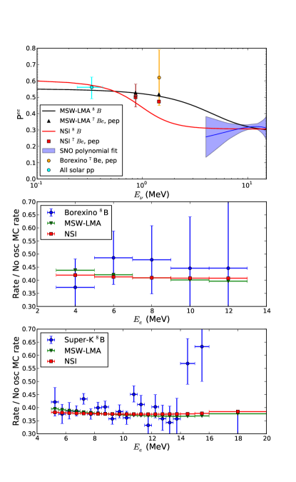
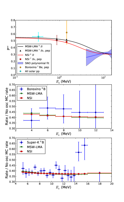
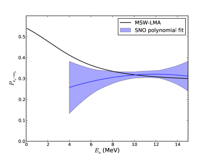
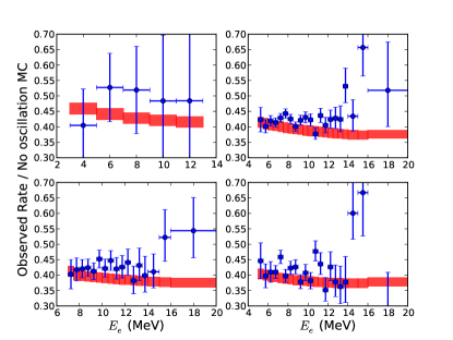
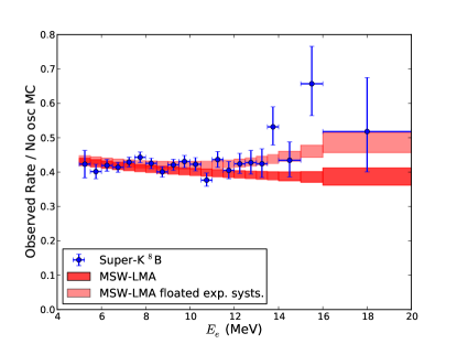
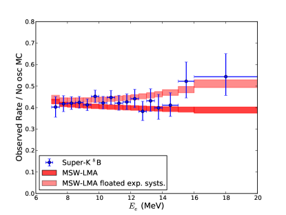
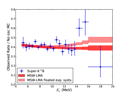
Many authors Friedland et al. (2004); Guzzo et al. (2002); Miranda et al. (2006); Palazzo (2011); Barger et al. (2005); Cirelli et al. (2005); Gonzalez-Garcia et al. (2006); Gonzalez-Garcia and Maltoni (2008); Gonzalez-Garcia et al. (2007) have put forth non-standard models and performed fits to the solar neutrino data set. Prior to the recent $\theta_{13}$ measurements, Palazzo Palazzo (2011) showed that non-standard interaction models provide a somewhat better fit to the solar neutrino data than does the standard MSW flavor transformation. The reason non-standard effects are preferred is the frustratingly persistent flatness of the high-energy solar $\nu_{e}$ survival probability, as measured by experiments observing ⁸B neutrinos. In Figs. 2 and 3, we show the ⁸B measurements from the Sudbury Neutrino Observatory (SNO), Borexino, and the Super-Kamiokande (S-K) experiments, with the expectation from large-mixing angle MSW effect superimposed. We see that while the data is consistent with MSW, no experiment sees clear evidence of the expected rise due to the matter / vacuum transition region. The three experiments appear to differ in their comparison to the model: SNO fits the prediction best at high energies rather than low, while S-K is the reverse. In other words, SNO’s data appears to be flatter than predicted by MSW due to the fact that at low energies the survival probability fit is lower than the MSW curve, while S-K’s data appears to be flatter because the high energy event rate is higher than predicted by MSW, but in all cases the end result is that the data appears flatter than expected. The Borexino experiment’s uncertainties are clearly too large to make a meaningful comparison with their data alone.

Figure 2: (Color online) KamLAND’s combined best fit MSW-LMA prediction versus SNO extracted ${}^{8}B$ survival probability. The band represents the RMS spread at any given energy, i.e., not including energy correlations.

Figure 3: (Color online) Top left: Borexino, top right: S-K I, bottom left: S-K II, bottom right: S-K III. Event rates binned in measured electron energy with each bin scaled by Monte Carlo predictions assuming GS98SF2 fluxes, versus the same ratio for the expected rates assuming KamLAND’s combined best fit LMA parameters and SNO’s NC ${}^{8}B$ flux prediction. Error bars on the data points represent statistical and energy uncorrelated systematic uncertainties combined in quadrature. Detector response parameters have been fixed at their reported value; the width of the band does not include the effect of correlated systematic uncertainties. The best fit oscillation prediction band width represents the uncertainty on the ⁸B flux. Note that we have suppressed the zero for these figures to better illustrate the comparison between data and model.

In this paper we perform fits to the global solar neutrino data sets, including constraints on $\theta_{13}$ and the most recent measurements by the SNO collaboration. Section II describes each experiment we consider, how we simulate its results, and how we handle its statistical and systematic uncertainties. Section III describes our fitting procedure and our parameterization of the survival probability for each model we consider, and the results of the fit for each model are given in Section IV.

II Data Sets and Approach

Our solar neutrino data sets include the weighted average of the results of the gallium experiments (SAGE, GALLEX, and GNO) given in Ref. Abdurashitov et al. (2009), and separately the results of the Chlorine experiment Cleveland et al. (1998). These experiments provide integral measurements of several solar neutrino fluxes. For the ‘realtime’ experiments, which measure exclusive fluxes, we include the most recent SNO results Aharmim et al. (2011) for ⁸B, the measurements of S-K I Hosaka et al. (2006), S-K II Cravens et al. (2008), and S-K III Abe et al. (2011b) (which are also ⁸B), and the measurements of Borexino for ⁷Be Bellini et al. (2011), ⁸B Bellini et al. (2010), and $pep$ Bellini et al. (2012).

We follow the standard approach taken by other authors, except for the handling of the SNO results, for which explicit energy-dependent survival probabilities are provided. For all data sets other than SNO we predict the expected number of events either in a given energy bin or as an integral flux. To achieve this we convolve the neutrino energy spectrum with its interaction cross section on a given target, and the outgoing electron energy with the detector’s response. For a given oscillation hypothesis, we include in this integral the energy dependence of the survival probability. Because of the dependence on the production region within the Sun we calculate the survival probabilities separately for each solar neutrino source. The Super-Kamiokande collaboration has provided bin-by-bin “no-oscillation” spectra that include their full Monte Carlo detector model. Therefore for a given oscillation hypothesis we scale their numbers by the ratio of oscillation to no-oscillation calculated using the analytic Gaussian response they have provided.

Our survival probability calculation is an analytical approximation to a full three-flavor numerical integration of the wave equation. We assume in all cases that $\Delta m^{2}_{31}/E$ is much larger than $\Delta m^{2}_{21}/E$ or any matter potential so the third flavor decouples and propagates independently of the other two. In addition, we assume adiabatic propagation in the Sun corrected by a two-flavor jump probability calculated at the resonance of maximal adiabaticity violation Parke (1986) (the results agree well with numerical calculations). We integrate over production location in the Sun for high metallicity model GS98SF2 Grevesse and Sauval (1998) and low metallicity model AGSS09SF2 Asplund et al. (2009), using neutrino production and solar density distributions from each Serenelli et al. (2011). For the day-night effect we use the procedure described in Ref. Akhmedov et al. (2004), modeling the Earth as two spherical shells of constant density. We use a parameterized average annual solar exposure as described in Ref. Lisi and Montanino (1997). Although we float the mixing parameters in our fits to data, we constrain them by known terrestrial measurements. For the dominant $\theta_{12}$ and $\Delta m^{2}_{21}$ parameters we use constraints from KamLAND Gando et al. (2011), and constrain $\theta_{13}$ by the results of the Daya Bay An et al. (2013) and RENO Ahn et al. (2012) collaborations.

Interaction cross sections for the Chlorine experiment are taken from Bahcall Bahcall et al. (1996), including the estimated theoretical uncertainties. For the Gallium experiments, we assume zero strength for capture to the first two excited states of ⁷¹Ge, as given in Appendix C of Ref. Abdurashitov et al. (2009) of the SAGE collaboration. The remaining cross section has uncertainties that are highly asymmetric for certain energies. We follow Bahcall’s suggestion Bahcall (1997) and take a conservative approach that treats uncertainties for energies above 2 MeV and uncertainties below 2 MeV as being correlated with each group but not with each other. To handle the asymmetric nature of the uncertainties, we use a bifurcated Gaussian. For the elastic scattering cross section of electrons, which applies to Borexino and Super-Kamiokande, we use the cross section that includes radiative and electroweak corrections as given by Bahcall Bahcall et al. (1995).

We consider all experimental uncertainties to be independent, with the exception of the three S-K measurements for which we treat the normalization uncertainties as being correlated across the three data sets. We have marginalized over systematic uncertainties for each experiment.

For Chlorine, Gallium, and Borexino, we check our reproduction of their data by comparing their no-oscillation flux predictions to our calculations. Borexino only gives a prediction for their integral measurement, but as mentioned earlier S-K provides binned no-oscillation predictions, allowing us to check our calculations more carefully. The binned predictions differ from our calculations by around a few percent per bin, which we assume to be due to unreported differences between the Gaussian detector response given in Ref. Abe et al. (2011b) and their full detector Monte Carlo. Once we scale our binned data by these differences, our integral flux predictions match within one percent.

For the results of the SNO collaboration, we can conveniently use the $\nu_{e}$ survival probability directly. To test a given oscillation hypothesis against the SNO survival probability, we use the prescription described in Refs. Aharmim et al. (2010) and Aharmim et al. (2011). The survival probability is projected onto the detected ⁸B spectrum, and the quadratic form used by the SNO collaboration is extracted. In this way, the comparison comes down to a test of just six parameters: three for the day survival probability,

$$P^{day}_{ee}(E_{\nu} = c_{0}+c_{1}(E_{\nu}[\text{MeV}]-10)$$ (1)

$$+c_{2}(E_{\nu}[\text{MeV}]-10)^{2},$$

two for the day-night asymmetry,

$$A_{ee}(E_{\nu}=a_{0}+a_{1}(E_{\nu}[\text{MeV}]-10),$$ (2)

and one for the ⁸B flux scale.

III Fit

Our interest is in reasonably generic non-standard models, especially those with the ability to flatten the ⁸B survival probability. For this analysis we have chosen three types of models: non standard contributions to forward scattering as described in Friedland et al. (2004), mass varying neutrinos Barger et al. (2005), and long-range leptonic forces Gonzalez-Garcia et al. (2007).

We used these models to calculate survival probabilities, including the dominant standard MSW-LMA oscillation. We perform a maximum likelihood fit to the data, floating the standard mixing parameters ($\theta_{12},\Delta m^{2}_{21},\theta_{13}$) and various non-standard parameters for each model as well as the flux scaling for each neutrino production reaction and a systematic parameter for the shape of the ⁸B spectrum Bahcall et al. (1996). Where we reference $\chi^{2}$ in this paper we mean $-2\log\mathcal{L}$. We constrain the values of the known mixing parameters to the values measured by the KamLAND collaboration Gando et al. (2011) for the (1,2) sector, and the measurements of KamLAND, Daya Bay, and RENO for $\theta_{13}$. The flux for each neutrino production reaction is constrained by the standard solar model values and uncertainties, although for ⁸B the main constraint instead comes from SNO’s NC measurement.

III.1 Non-Standard Forward Scattering

As suggested by Friedland in Friedland et al. (2004), one can generically parameterize these non-standard contributions with an effective low-energy four-fermion operator

$$\mathcal{L}=-2\sqrt{2}G_{F}(\bar{\nu}_{\alpha}\gamma_{\rho}\nu_{\beta})(\epsilon^{f\tilde{f}P}_{\alpha\beta}\bar{f}_{P}\gamma^{\rho}\tilde{f}_{P})+h.c.,$$ (3)

where P=L,R, and $\epsilon^{f\tilde{f}P}_{\alpha\beta}$ denotes the strength of the non-standard interaction between neutrinos of flavors $\alpha$ and $\beta$ and the P handed components of fermions $f$ and $\tilde{f}$. Only vector components where $f=\tilde{f}$ of the non-standard interaction can affect the neutrino propagation, so we let $\epsilon^{f}_{\alpha\beta}\equiv\epsilon^{ffL}_{\alpha\beta}+\epsilon^{ffR}_{\alpha\beta}$. One can define $\epsilon_{\alpha\beta}=\sum_{f=u,d,e}\epsilon^{f}_{\alpha\beta}n_{f}/n_{e}$. Then the matter part of the generic three flavor NSI oscillation Hamiltonian can be written as

$$\mathcal{H}=\sqrt{2}G_{F}n_{e}\begin{pmatrix}1+\epsilon_{ee}&\epsilon^{*}_{e\mu}&\epsilon^{*}_{e\tau}\\ \epsilon_{e\mu}&\epsilon_{\mu\mu}&\epsilon^{*}_{\mu\tau}\\ \epsilon_{e\tau}&\epsilon_{\mu\tau}&\epsilon_{\tau\tau}\end{pmatrix}.$$ (4)

As in our standard survival probability calculation, we assume the third flavor decouples and that the non-standard contribution to the potential is much smaller than $\Delta m^{2}_{31}/E$. Then the effective two flavor Hamiltonian is

$$\textbf{H}^{2\nu}= \frac{\Delta m^{2}_{21}}{4E}\begin{pmatrix}-\cos 2\theta_{12}&\sin 2\theta_{12}\\ \cos 2\theta_{12}&\sin 2\theta_{12}\end{pmatrix}$$ (5)

$$+\sqrt{2}G_{f}n_{e}\begin{pmatrix}\cos\theta_{13}&\epsilon_{1}^{*}\\ \epsilon_{1}&\epsilon_{2}\end{pmatrix}$$

where

$$\epsilon_{1} = c_{13}(\epsilon_{e\mu}c_{23}-\epsilon_{e\tau}s_{23})$$ (6)

$$-s_{13}[\epsilon_{\mu\tau}s^{2}_{23}-\epsilon^{*}_{\mu\tau}c^{2}_{23}+(\epsilon_{\mu\mu}-\epsilon_{\tau\tau})c_{23}s_{23}],$$

$$\epsilon_{2} = \epsilon_{\mu\mu}c^{2}_{23}-(\epsilon_{\mu\tau}+\epsilon^{*}_{\mu\tau})s_{23}c_{23}+\epsilon_{\tau\tau}s^{2}_{23}$$ (7)

$$+c^{2}_{13}\epsilon_{ee}+s_{13}[(e^{-i\delta}\epsilon_{e\mu}+e^{i\delta}\epsilon^{*}_{e\mu})s_{23}c_{13}$$

$$+(e^{-i\delta}\epsilon_{e\tau}+e^{i\delta}\epsilon^{*}_{e\tau})c_{13}c_{23}]$$

$$-s^{2}_{13}[\epsilon_{\mu\mu}s^{2}_{23}+(\epsilon_{\mu\tau}+\epsilon^{*}_{\mu\tau})s_{23}c_{23}+\epsilon_{\tau\tau}c^{2}_{23}].$$

We follow the example of Ref. Friedland et al. (2004) to calculate a modified mixing angle in matter as well as a jump probability to get a predicted survival probability.

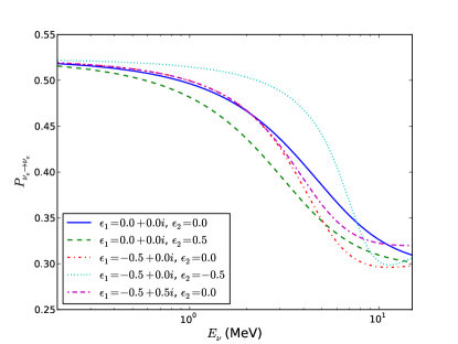
This model adds up to three new parameters to the survival probability: $Re[\epsilon_{1}],Im[\epsilon_{1}],\epsilon_{2}$. Fig. 4 shows the effect of each one on the shape of the survival probability.

Figure 4: (Color online) Survival probabilities for a range of the NSI parameters $\epsilon_{1},\epsilon_{2}$

Current constraints on the strength of these vertices come from accelerator experiments like NuTeV and CHARM, atmospheric neutrino and charged lepton experiments like LEP, and by limits on the charged lepton operators. The parameters $\epsilon_{e\mu},\epsilon_{\mu\mu}$ are well constrained ($\lower 2.0pt\hbox{$\,\buildrel\scriptstyle<\over{\scriptstyle\sim}\,$}10^{-2}-10^{-3}$), and analysis of atmospheric neutrino data has shown $\epsilon_{\mu\tau}\lower 2.0pt\hbox{$\,\buildrel\scriptstyle<\over{\scriptstyle\sim}\,$}10^{-2}$ Gonzalez-Garcia and Maltoni (2008). However there remain vertices that can still be quite large, for example, $|\epsilon^{f}_{e\tau,ee}|\lower 2.0pt\hbox{$\,\buildrel\scriptstyle<\over{\scriptstyle\sim}\,$}0.5$, or $|\epsilon^{dR}_{tt}|<6$.

By letting all the muon vertices go to zero, we get

$$\epsilon_{1} = -c_{13}s_{23}\epsilon_{e\tau}+s_{13}c_{23}s_{23}\epsilon_{\tau\tau},$$ (8)

$$\epsilon_{2} = s^{2}_{23}\epsilon_{\tau\tau}+c^{2}_{13}\epsilon_{ee}+s_{13}c_{13}c_{23}(e^{-i\delta}\epsilon_{e\tau}+e^{i\delta}\epsilon_{e\tau}^{*})$$ (9)

$$-s^{2}_{13}c^{2}_{23}\epsilon_{\tau\tau}.$$

The effect of these non-standard parameters on the survival probability as a function of energy is shown in Fig. 4.

III.2 Mass Varying Neutrinos

III.2.1 Neutrino Density Effects

In Ref. Barger et al. (2005) it was proposed that neutrinos are coupled to dark energy in a way that their energy densities track each other. This model was made to resolve the coincidence of the energy density of dark energy and matter being similar today even though their ratio scales as $\sim$1/(scale factor)³. In general this implies so-called ‘Mass Varying Neutrinos’ (MaVaNs), where the neutrino mass becomes a function of the neutrino density. If the neutrino couples to a scalar field, then following Ref. Cirelli et al. (2005) at low energy one can write an effective Lagrangian in a model independent way

$$\textbf{L}(m_{i})= \sum_{i}\left[m_{i}\overline{\nu}^{c}_{i}\nu_{i}+m_{i}n_{i}^{C\nu B}\right.$$

$$\left.+\int\frac{d^{3}k}{(2\pi)^{3}}\sqrt{k^{2}+m_{i}^{2}}f_{i}(k)+V_{0}(m_{i})\right].$$ (10)

Here $n_{i}^{C\nu B}=112$ cm^-3 is the number density of non-relativistic relic neutrinos of each type and $f_{i}(k)$ is the occupation number for momentum k of non-relic neutrinos in our medium (in this case a function of the neutrino production profile in the Sun). Then one can parameterize the scalar potential $V_{0}(m_{i})\propto f(m_{i}/\mu)$ where $\mu$ is some arbitrary mass scale. The observed equation of state for dark energy implies that the potential must be flat, while minimizing the total potential implies it must decrease with increasing neutrino mass. Various forms for the scalar potential have been suggested, for example, $\log(\mu/m_{i})$ or $(m_{i}/\mu)^{-\alpha}$. For either of these forms, minimizing the effective potential implies that

$$m_{i}(r)\approx m_{i,0}-|U_{e,i}|^{2}A(r)m_{i,0}^{2},$$ (11)

where $m_{i,0}$ is the vacuum mass of $\nu_{i}$ and

$$A(r)=\frac{1}{n^{C\nu B}}\int\frac{d^{3}k}{(2\pi)^{3}}\frac{1}{\sqrt{k^{2}+m_{i}^{2}}}f_{e}(k,r).$$ (12)

Here we have used the fact that $f_{i}(k,r)=|U_{e,i}|^{2}f_{e}(k,r)$ Cirelli et al. (2005).

Then before MSW matter effects, we have

$$\Delta m^{2}_{21,eff}(r) = m_{2}^{2}(r)-m_{1}^{2}(r)$$ (13)

$$\approx \Delta m^{2}_{21,0}\left[1-3s^{2}_{12}c^{2}_{13}A(r)m_{1,0}\right]$$

$$+2c^{2}_{13}A(r)\left[c^{2}_{12}-s^{2}_{12}\right]m_{1,0}^{3},$$

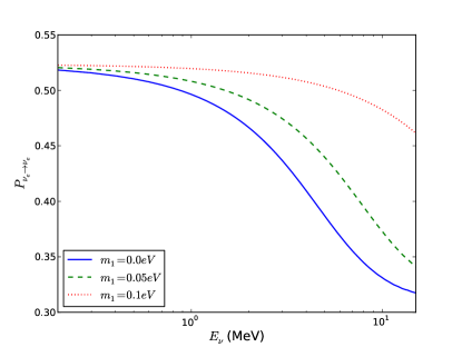
and we can solve for the survival probability by substituting this effective mass squared difference into the survival probability calculations for normal MSW oscillations. Then given a particular distribution of neutrinos, our effective mass squared difference becomes a function of the vacuum neutrino mass $m_{1,0}$. The survival probability for various values of the vacuum mass is shown in Fig. 5.

A previous two-flavor oscillation analysis of solar data and KamLAND found a $3\sigma$ upper limit of $m_{1,0}<0.009$ eV, with no improvement in the fit to the data over MSW-LMA Cirelli et al. (2005).

Figure 5: (Color online) Survival probabilities for the neutrino density dependent MaVaN model at several values of $m_{1,0}$

III.2.2 Fermion Density Effects

In addition to the effect described above, it is possible for this scalar field to couple to visible matter. Ref. Gonzalez-Garcia et al. (2006) parameterizes this model by adding a light scalar field $\phi$ of mass $m_{\phi}$, which is weakly coupled to neutrinos and fermions;

L $$= \sum_{i}\overline{\nu}_{i}(i\not{\partial}-m_{i,0})\nu_{i}+\sum_{f}\overline{f}(i\not{\partial}-m_{f,0})f$$ (14)

$$+\frac{1}{2}\phi(\partial^{2}-m_{\phi}^{2})\phi+\sum_{ij}\lambda^{ij}\overline{\nu}_{i}\nu_{j}\phi$$

$$+\sum_{f}\lambda^{f}\overline{f}f\phi.$$

Then the elements of the mass matrix become

$$m_{ij}(r) = m_{i,0}\delta_{ij}-M_{ij}(r),$$

$$M_{ij}(r) = \frac{\lambda^{ij}}{m_{\phi}^{2}}\left(\sum_{f}\lambda^{f}n_{f}(r)\right.$$ (15)

$$\left.+\sum_{i}\lambda^{ii}\int\frac{d^{3}k}{(2\pi)^{3}}\frac{M_{ii}}{\sqrt{k^{2}+M^{2}_{ii}}}f_{i}(k,r)\right).$$

We will only consider the added effect of the coupling to fermionic matter by letting $m_{1,0}\sim 0$, such that

$$M_{ij}(r)=\frac{\lambda^{ij}}{m_{\phi}^{2}}\sum_{f}\lambda^{f}n_{f}(r).$$ (16)

Assuming that effect of this coupling is small compared to $m_{3,0}$, we can decouple the third neutrino state. Then diagonalizing the 1-2 sector for the mass eigenstates in matter gives

$$\cos 2\theta^{m}_{12}(r_{0})=\frac{2\Delta m^{2}_{21}(r)\cos 2\theta_{12}-A(r)}{\Delta m^{2}_{m}}$$ (17)

where

$$\Delta m^{2}_{m} = \left((\Delta m^{2}_{21}(r))^{2}+4M_{3}^{4}(r)\right.$$ (18)

$$\left.-2A(r)\Delta m^{2}_{21}(r)\cos 2\theta_{12}+A^{2}\right)^{\frac{1}{2}},$$

$$\Delta m^{2}_{21}(r) = (m_{2,0}-M_{2}(r))^{2}-(m_{1,0}-M_{1}(r))^{2},$$ (19)

and $M_{1,2,3}$ are linear combinations of the $M_{ij}$s, and can be parameterized as

$$M_{i}(r)=\alpha_{i}\rho(r)$$ (20)

for matter density $\rho(r)$. Then we can substitute the mixing angle in matter from Eq. 17 into our standard oscillation equations to get a survival probability as a function of our parameters $\alpha_{i}$.

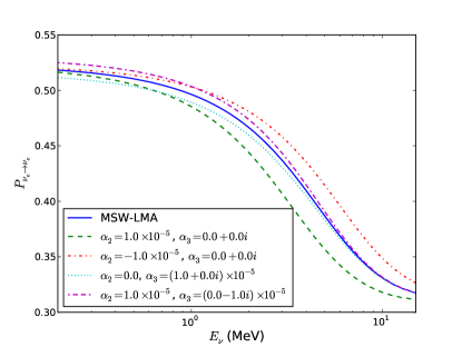
For the KamLAND constraint, we replace $\theta_{12}$ with $\theta_{12}^{m}$ and $\Delta m^{2}_{21}$ with $\Delta m^{2}_{m}$ as defined above except with $A\to-A$ and $\rho\sim 3$gr/cm³ for the density of the Earth’s crust. The survival probability for various values of the parameters $\alpha_{i}$ is shown in Fig. 6.

Current limits for the effective Yukawa coupling of any scalar with $m_{\phi}\lower 2.0pt\hbox{$\,\buildrel\scriptstyle>\over{\scriptstyle\sim}\,$}10^{-11}$eV to nucleons from tests of the inverse square law are $|\lambda^{N}|\lower 2.0pt\hbox{$\,\buildrel\scriptstyle<\over{\scriptstyle\sim}\,$}10^{-21}$ [22]. A previous two-flavor oscillation analysis of solar data plus KamLAND Gonzalez-Garcia et al. (2006) found 90% confidence level bounds of

$$-2.2\times 10^{-5}\leq \alpha_{2}/\text{eV} \leq 1.4\times 10^{-4},$$ (21)

$$|\alpha_{3}|/\text{eV} \leq 2.3\times 10^{-5}\text{ for }\alpha_{3}^{2}>0,$$ (22)

$$|\alpha_{3}|/\text{eV} \leq 3.4\times 10^{-5}\text{ for }\alpha_{3}^{2}<0.$$ (23)

Figure 6: (Color online) Survival probabilities for the fermion density dependent MaVaN model at several values of $\alpha_{2},\alpha_{3}$

III.3 Long-Range Leptonic Forces

We consider another group of generic non-standard interactions characterized by a new long-range force coupling to lepton flavor number. Since lepton flavor number is not conserved, such a force is likely to have a finite range. In general if the range is long enough, we follow Ref. Gonzalez-Garcia et al. (2007) and write the effect of the force at some point in the Sun in terms of a function

$$W(r)=\frac{2\pi\lambda}{r}\int_{0}^{R_{sun}}dr^{\prime}r^{\prime}n_{e}(r^{\prime})\left(e^{-|r^{\prime}-r|/\lambda}-e^{-(r^{\prime}+r)/\lambda}\right),$$ (24)

where $\lambda$ is the range of the force. Long range forces of this kind can be probed by studying experimental tests of the equivalence principle; this sort of analysis was used to get a bound on a vector long-range force’s dimensionless coupling constant $k_{V}<10^{-49}$ Okun (1996). More recently Gonzalez-Garcia et al Gonzalez-Garcia et al. (2007) performed a two flavor oscillation analysis of solar data to find $3\sigma$ bounds for scalar, vector, and tensor forces of infinite range that couple to electron number of

$$k_{S}(e) \leq 5.0\times 10^{-45}\text{ }(m_{1}=0\text{eV}),$$ (25)

$$k_{S}(e) \leq 1.5\times 10^{-46}\text{ }(m_{1}=0.1\text{eV}),$$ (26)

$$k_{V}(e) \leq 2.5\times 10^{-53},$$ (27)

$$k_{T}(e) \leq 1.7\times 10^{-60}\text{eV}^{-1}.$$ (28)

III.3.1 Scalar Interaction

In the case where the new long-range force is a scalar coupling, we see a similar situation to the MaVaN. We now have a light scalar that only couples to neutrinos and electrons, which one can parameterize in terms of the function W(r). The new term in the Lagrangian for the neutrinos is

$$\textbf{L}=-g_{0}\phi\overline{\nu}\nu$$ (29)

and so the kinetic part of the Hamiltonian gains a term

$$\textbf{M}^{\prime}=U_{12}^{\dagger}U_{13}^{\dagger}U_{23}^{\dagger}\begin{pmatrix}-M_{s}(r)&0&0\\ 0&0&0\\ 0&0&0\end{pmatrix}U_{23}U_{13}U_{12},$$ (30)

where $M_{s}(r)=k_{s}(e)W(r)$ and $k_{s}(e)=\frac{g_{0}^{2}}{4\pi}$. After decoupling the third flavor and diagonalizing the mass matrix for the remaining two we get the matter mixing angle in the adiabatic limit of

$$\sin 2\theta^{m}_{12}(r_{0})=\frac{\sin 2\theta_{12}\Delta m^{2}_{s}}{\Delta m^{\prime 2}_{s}}$$ (31)

where

$$\Delta m^{2}_{s} = \Delta m^{2}_{12}-M_{s}(r_{0})\Delta m_{12}c^{2}_{13},$$ (32)

$$(\Delta m^{\prime 2}_{s})^{2} = \left[\Delta m^{2}_{s}\cos 2\theta_{12}-2E_{\nu}V(r_{0})c^{2}_{13}\right.$$ (33)

$$\left.-M_{s}^{2}(r_{0})c^{2}_{13}+M_{s}(r_{0})(m_{1}+m_{2})\right]^{2}$$

$$+\sin 2\theta_{12}\Delta m^{2}_{s}.$$

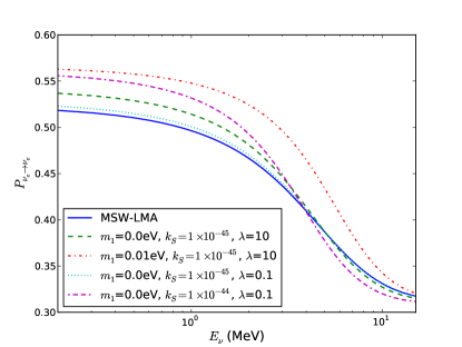
The survival probability for various values of the range and coupling strength is shown in Fig. 7.

Figure 7: (Color online) Survival probabilities for a long-range scalar interaction at various values of the range and strength of the coupling and the neutrino mass scale.

III.3.2 Vector Interaction

If the force is mediated by a vector boson $A_{\alpha}$, then

$$\textbf{L}=-g_{1}A_{\alpha}\overline{\nu}\gamma^{\alpha}\nu$$ (34)

and the potential $V(r)=V_{MSW}+k_{V}W(r)$ where $k_{V}=\frac{g_{1}^{2}}{4\pi}$. We can solve for the survival probability using the standard MSW oscillation equations, substituting in the above for the MSW potential.

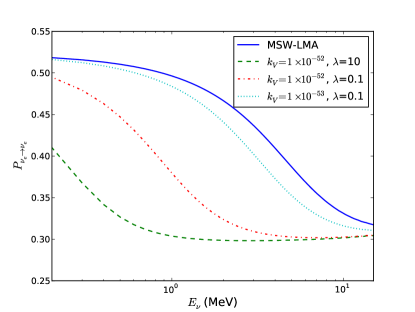
The survival probability for various values of the range and coupling strength is shown in Fig. 8.

Figure 8: (Color online) Survival probabilities for a long-range vector interaction at various values of the range and strength of the coupling.

III.3.3 Tensor Interaction

If the force is mediated by a tensor field with spin 2, $\chi_{\alpha\beta}$, then

$$\textbf{L}=-\frac{g_{2}}{2}\chi_{\alpha\beta}\left(\overline{\nu}\gamma^{\alpha}i\partial^{\beta}\nu-i\partial^{\alpha}\overline{\nu}\gamma^{\beta}\nu\right).$$ (35)

Now the potential is $V(r)=V_{MSW}+E_{\nu}k_{T}W(r)$, where $k_{T}=m_{e}\frac{g_{2}^{2}}{4\pi}$. Again we can use the standard MSW oscillation equations substituting in this new potential.

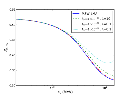
The survival probability for various values of the range and coupling strength is shown in Fig. 9.

Figure 9: (Color online) Survival probabilities for a long-range tensor interaction at various values of the range and strength of the coupling.

III.4 Non-Standard Solar Model

We want to check that any improvement in the fit achieved by replacing MSW with a non-standard model cannot be easily reproduced by modifying solar model parameters. In addition, we want to see that we are sensitive to the transition region independent of exact knowledge of the Sun — that is, that small changes in the parameters of the solar model do not create changes in the transition region on the order of the small effects expected from non-standard models. To this end, in addition to comparing fits using both the high metallicity and low metallicity solar models, we use the fact that in the adiabatic approximation, there are only two inputs from the solar model that affect the survival probability. They are the absolute flux constraints, and the convolution of the density profile with the neutrino production profiles. We can effectively remove many of our assumptions about the solar model from our fit by removing the absolute flux constraints entirely, and for the other two sets of parameters, distorting the density profile linearly, so that

$$n_{e}^{\prime}(r)=(1+\delta_{0}+\alpha r)n_{e}(r)$$ (36)

for some change in the core density $\delta_{0}$, where $\alpha$ is determined by $\delta_{0}$ and the constraint that the total mass remains the same. A recent study has shown that a change in the central density is plausible, and was able to create a model with the central density increased by over 10% using stellar evolution software Lopes and Turck-Chièze (2013).

We can get a reasonable constraint on the uncertainty of the solar density profile by comparing the predictions of standard solar models to helioseismological measurements of the sound profile, which differ by around 1% Bahcall et al. (2006, 2005).

In this fit we will not constrain the density change since we are also using it as a proxy for any change in the production profile. Additionally, although we cannot use the flux constraints from the solar model in this fit since they are no longer valid once we change the density, we can constrain the sum of the fluxes using the luminosity of the Sun Bahcall (2002) and constrain the ratio of the $pp$ to $pep$ fluxes since the nuclear matrix elements are the same Gonzalez-Garcia et al. (2010).

IV Results

IV.1 Large Mixing Angle MSW

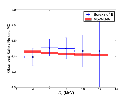
We find the best fit point for standard MSW-LMA at $\Delta m^{2}_{21}=7.462\times 10^{-5}$ eV${}^{2},\sin^{2}\theta_{12}=0.301,\sin^{2}\theta_{13}=0.0242$, with a ⁸B flux of $5.31\times 10^{6}$ cm^-2s^-1. The fit compared to the data sets of SNO, Borexino, and S-K is shown in Figs. 10-14. Although in general for the analyses in this paper we marginalize over S-K’s systematic uncertainties, it is important to note how they affect the goodness of the fit. To show this effect, we plot the observed rate in S-K against the predicted rate calculated from our best fit mixing parameters in two ways: first fixing the energy scale, energy resolution, and efficiency to the values reported by S-K, and second using values for these parameters obtained by floating them in our fit. In both cases the width of the band does not include any of the systematic uncertainties associated with these parameters since they are energy dependent and so cannot be captured in a single plot. We find the best fit with the energy scale at $+1.1\sigma$, the energy resolution at $-1.0\sigma$ and the overall efficiency at $+0.6\sigma$. The efficiency systematic uncertainty increases the average predicted ratio while the other two each bend up the high energy end of the spectrum. In other words, while the LMA prediction appears to be a poor fit to the high-energy region of the S-K data, the allowed variation from S-K’s systematic uncertainties can explain the difference if they are moved roughly 1$\sigma$ from their central values. Better constraints on the S-K detector response parameters might therefore lead to a more significant disagreement with the LMA model.

Figure 10: (Color online) Our best fit MSW-LMA prediction versus SNO extracted ${}^{8}B$ survival probability. The band represents the RMS spread at any given energy, i.e., not including energy correlations.

Figure 11: (Color online) Borexino event rate binned in measured electron energy with each bin scaled by Monte Carlo predictions assuming GS98SF2 fluxes, versus the same ratio for the expected rates assuming our best fit LMA parameters and fluxes. Error bars on the data points represent statistical uncertainties only. The best fit oscillation prediction band width represents the uncertainty on the ⁸B flux.

Figure 12: (Color online) S-K I event rates binned in measured electron energy with each bin scaled by Monte Carlo predictions assuming GS98SF2 fluxes, versus the same ratio for the expected rates assuming our combined best fit LMA parameters and fluxes. Error bars on the data points represent statistical and energy uncorrelated systematic uncertainties combined in quadrature. The two bands show the effect of the correlated systematic uncertainties: for the dark band, detector response parameters have been fixed at their reported values, while for the light they have been floated in the fit. The best fit oscillation prediction band width represents the uncertainty on the ⁸B flux.

Figure 13: (Color online) S-K II event rates binned in measured electron energy with each bin scaled by Monte Carlo predictions assuming GS98SF2 fluxes, versus the same ratio for the expected rates assuming our combined best fit LMA parameters and fluxes. Error bars on the data points represent statistical and energy uncorrelated systematic uncertainties combined in quadrature. The two bands show the effect of the correlated systematic uncertainties: for the dark band, detector response parameters have been fixed at their reported values, while for the light they have been floated in the fit. The best fit oscillation prediction band width represents the uncertainty on the ⁸B flux.

Figure 14: (Color online) S-K III event rates binned in measured electron energy with each bin scaled by Monte Carlo predictions assuming GS98SF2 fluxes, versus the same ratio for the expected rates assuming our combined best fit LMA parameters and fluxes. Error bars on the data points represent statistical and energy uncorrelated systematic uncertainties combined in quadrature. The two bands show the effect of the correlated systematic uncertainties: for the dark band, detector response parameters have been fixed at their reported values, while for the light they have been floated in the fit. The best fit oscillation prediction band width represents the uncertainty on the ⁸B flux.

IV.2 Non-Standard Forward Scattering

We formulate our results for this section to be comparable to Palazzo Palazzo (2011), so $\epsilon^{e}_{\alpha\beta}=\epsilon^{u}_{\alpha\beta}=0$. For a more general case to first order $n_{f}/n_{e}$ can be considered constant in the Sun, thus any combination of $\epsilon^{e,u,d}$’s would just be a scaling of our results.

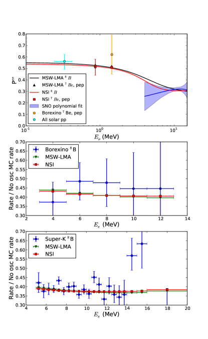
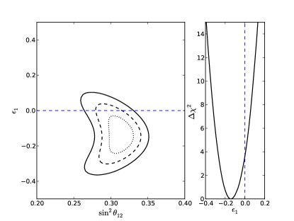
First we consider only real $\epsilon_{1}$ with $\epsilon_{2}=0$. Including the most up-to-date solar results and the most recent KamLAND results as a constraint, letting $\theta_{12}$ and $\Delta m^{2}_{12}$ float and fixing $\theta_{13}=0$, we get a best fit of $\epsilon_{1}=-0.137^{+0.070}_{-0.071}$, shown in Fig. 15, which well matches results from Palazzo. After letting $\theta_{13}$ float and adding in the constraint from RENO and Daya Bay, the significance becomes smaller, with a best fit value of $\epsilon_{1}=-0.145^{+0.118}_{-0.109}$, shown in Figs. 16 and 17. The best fit survival probability compared to MSW-LMA and to data considered in this analysis is shown in the appendix in Fig. 27.

Figure 15: Left: Two flavor contours with $\epsilon_{2}=0$ and real $\epsilon_{1}$. Contours are shown for 68%, 95%, and 99.73% confidence levels for 2 d.o.f., where the $\chi^{2}$ has been minimized with respect to all undisplayed parameters. Right: $\Delta\chi^{2}$ as a function of $\epsilon_{1}$.

Figure 16: Left: Three flavor contours including constraints from RENO and Daya Bay. Contours are shown for 68%, 95%, and 99.73% confidence levels for 2 d.o.f., where the $\chi^{2}$ has been minimized with respect to all undisplayed parameters. Right: $\Delta\chi^{2}$ as a function of $\epsilon_{1}$.

Figure 17: Three flavor contours including constraints from RENO and Daya Bay for $\epsilon_{1}$ and $\theta_{13}$. Contours are shown for 68%, 95%, and 99.73% confidence levels for 2 d.o.f., where the $\chi^{2}$ has been minimized with respect to all undisplayed parameters.

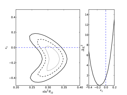
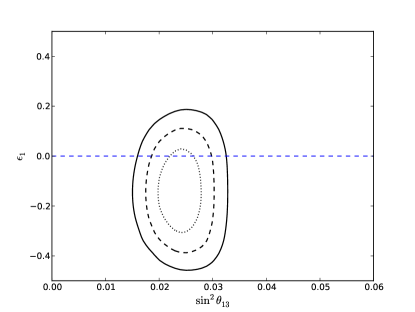
These results seem to allow a vacuum to matter transition in the survival probability at higher energies than the SNO data suggests. It is important to consider the fit to the day night asymmetry, shown in Fig. 18 for SNO. The NSI does not have a large effect on the asymmetry, and so for both models the best fit does not fit the data well. The correlations between the asymmetry and the day survival probability translate this poor fit to an even broader allowed upturn, further limiting the significance of any flatness in the data. We show this effect by fitting the MSW-LMA predicted day-night asymmetry to Eq. 2 and then recalculating what the RMS spread in the day night survival probability would be after fixing $a_{0}$ and $a_{1}$ given the correlation matrix, as shown in 19.

Figure 18: (Color online) Day-Night asymmetry from SNO results compared to best fit MSW-LMA and NSI. The band represents the RMS spread at any given energy, i.e., not including energy correlations.

Figure 19: (Color) Day survival probability for SNO. The blue band shows the RMS spread from the best fit, and the green band shows the spread after the Day-Night asymmetry is fixed to the MSW-LMA prediction.

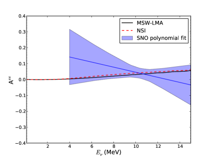
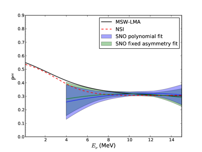
In addition, since these plots scale the absolute rates to get survival probabilities, they hide the relationship between the survival probability and the absolute flux. Both of these effects can be seen more clearly in the correlation matrix for SNO’s polynomial survival probability fit, Table VIII in Ref. Aharmim et al. (2011). The baseline level of the survival probability $c_{0}$ is strongly anticorrelated with the absolute flux $\Phi_{B}$, and the slope of the survival probability $c_{1}$ is anticorrelated with the slope of the day night asymmetry $a_{1}$.

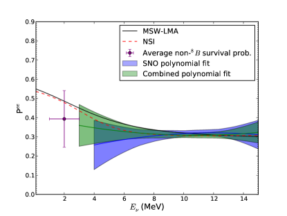
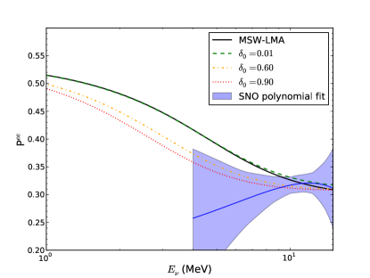
To better visualize why the full fit does not have a better constraint, we applied the polynomial survival probability fit as used for the SNO data to the combination of the SNO, S-K, Borexino, and Homestake results. This represents a fit to the survival probability independent of any physics model, where the polynomial forms in Eqs. 1 and 2 are used to impose an energy correlation under the model independent assumption that there is no small scale structure to the survival probability. Since the Homestake results could contain a significant fraction of non-⁸B events, one additional term for the average non-⁸B survival probability is added to the fit, where non-⁸B fluxes were fixed at SSM values. The results of the fit are given in Tables 1 and 2, and the best fit and RMS spread is shown in Fig. 20. The majority of the change from the SNO-only band is driven by the S-K results, where the high-energy end and the ${}^{8}B$ flux is pulled upward. Although their data looks flat in detected energy, when projected back into incident neutrino energy it becomes consistent with an LMA-like transition, as suggested in Figs. 12, 13, and 14. The band of the RMS spread shows the significance to which we can say anything about the the shape of the survival probability at low energies, and we can see that the band covers the MSW-LMA prediction but at the same time allows for a perfectly flat or even downward bending survival probability. Note that this combined polynomial fit does not impact any of the results in this paper since we are only using it to visualize the survival probability and do not actually use it in our likelihood fits.

	Best Fit	Fit Error
$\Phi_{B}$	5.403	0.195
$c_{0}$	0.309	0.015
$c_{1}$	-0.0014	0.0055
$c_{2}$	0.008	0.0022
$a_{0}$	0.047	0.020
$a_{1}$	0.000	0.018
$P_{\text{non-}^{8}B}$	0.393	0.148

Table 1: Results for polynomial fit for the survival probability and day-night asymmetry fit to the data of SNO, S-K, Borexino, and Homestake.

	$\Phi_{B}$	$c_{0}$	$c_{1}$	$c_{2}$	$a_{0}$	$a_{1}$	$P_{\text{non-}^{8}B}$
$\Phi_{B}$	1.000	-0.793	0.215	-0.152	-0.027	0.016	0.045
$c_{0}$	-0.793	1.000	-0.289	-0.279	-0.204	-0.009	-0.074
$c_{1}$	0.215	-0.289	1.000	-0.010	0.042	-0.587	0.023
$c_{2}$	-0.152	-0.279	-0.010	1.000	-0.032	-0.004	-0.073
$a_{0}$	-0.027	-0.204	0.042	-0.032	1.000	-0.073	0.014
$a_{1}$	0.016	-0.009	-0587	-0.004	-0.073	1.000	0.005
$P_{\text{non-}^{8}B}$	0.045	-0.074	0.023	-0.073	0.014	0.005	1.000

Table 2: Correlation matrix from the polynomial fit for the survival probability and day-night asymmetry fit to the data of SNO, S-K, Borexino, and Homestake.

Figure 20: (Color) Polynomial fit to SNO, Super-Kamiokande, Borexino ⁸B data and Homestake’s results. The band represents the RMS spread at any given energy, i.e., not including energy correlations.

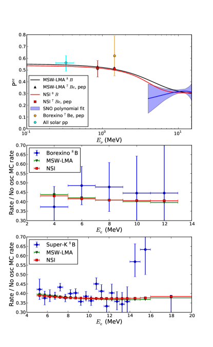
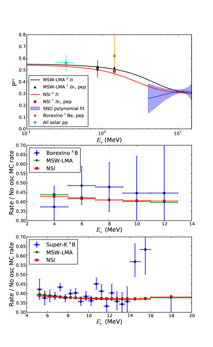
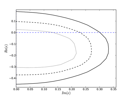
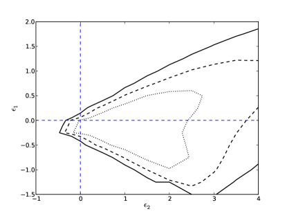
We also consider the case of complex $\epsilon_{1}$. Here the best fit is found at $\epsilon_{1}=-0.146+0.031i$. The fit results are shown in Fig. 21 and the best fit survival probability in the appendix in Fig. 28. For both $\epsilon_{1}$ and $\epsilon_{2}$ nonzero, we find the best fit point at $\epsilon_{1}=0.014,\epsilon_{2}=0.683$. The fit contours are shown in Fig. 22, and the best fit survival probability is shown in Fig. 29. In both cases the additional free parameter allows a slightly better fit, but the standard MSW-LMA is within the 68% confidence interval for two degrees of freedom. Once both $\epsilon_{1}$ and $\epsilon_{2}$ are allowed to be nonzero, there is no further improvement in the fit if we again let $\epsilon_{1}$ be complex.

For all of these scenarios, the best fit values for the non-standard parameters $\epsilon_{1}$ and $\epsilon_{2}$ are well within the current experimental bounds. At the same time, they represent relatively substantial effects, considering that at $\epsilon_{\alpha\beta}=1$ the non-standard interaction has the same strength as the MSW potential, as shown in Eq. 4.

Figure 21: Results for NSI fit with $\epsilon_{2}=0$ but complex $\epsilon_{1}$. Contours are shown for 68%, 95%, and 99.73% confidence levels (2 d.o.f.), where the $\chi^{2}$ has been minimized with respect to all undisplayed parameters.

Figure 22: Results for NSI fit with real $\epsilon_{1}$. Contours are shown for 68%, 95%, and 99.73% confidence levels (2 d.o.f.), where the $\chi^{2}$ has been minimized with respect to all undisplayed parameters.

IV.3 Mass Varying Neutrinos

IV.3.1 Neutrino Density Effects

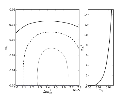
After fitting for $m_{1,0}$ letting all mixing parameters float, we found that the best fit point was at $m_{1,0}=0$, where this model’s predictions become identical to MSW-LMA. Our fit results, as shown in Fig. 23, give a 90% confidence level upper limit on the neutrino mass scale of $m_{1,0}<0.033$eV within this model. Our results do not agree with the previous limit in Cirelli et al. (2005), who found a limit an order of magnitude smaller. We cannot explain the difference, although they use older data sets for each experiment. For the inverted hierarchy we expect $m_{1,0}\lower 2.0pt\hbox{$\,\buildrel\scriptstyle>\over{\scriptstyle\sim}\,$}\sqrt{\Delta m^{2}_{atm}}\sim 0.05$ eV, so within the context of this model, the inverted hierarchy would be rejected.

Figure 23: Results for MaVaN model with neutrino mass coupled to neutrino density. Left: Contours are shown for 68%, 95%, and 99.73% confidence levels for 2 d.o.f., where the $\chi^{2}$ has been minimized with respect to all undisplayed parameters. Right: $\Delta\chi^{2}$ as a function of $m_{1,0}$.

IV.3.2 Fermion Density Effects

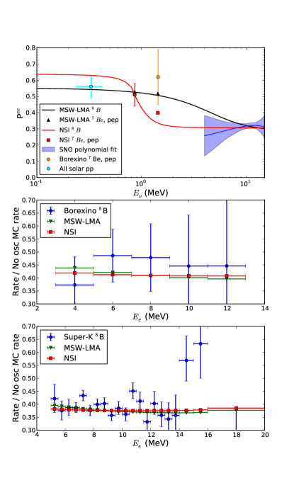
For simplification we let $m_{1,0}=\alpha_{1}=0$, so we fit for $\alpha_{2},Re[\alpha_{3}],Im[\alpha_{3}]$. Results for $\alpha_{2}>0$, $\alpha_{3}^{2}<0$ are shown in Fig. 24. In this case our best fit is at $\alpha_{2}=5.95\times 10^{-5}$, $\alpha_{3}=i1.97\times 10^{-5}$, shown in the appendix in Fig. 30, although the $2\sigma$ contour includes the origin. Note that although the ⁸B survival probability in Fig. 30 seems to be far from the Borexino $pep$ point, in this scenario the $pep$ survival probability is actually significantly different than ⁸B’s at the same energy, making it more consistent with the data than it would appear. Minimizing over all other variables gives the bounds at 90% confidence for 1 d.o.f. of

$$1.6\times 10^{-6}\leq \alpha_{2}/\text{eV} \leq 1.3\times 10^{-4},$$ (37)

$$|\alpha_{3}|/\text{eV} \leq 2.48\times 10^{-5}\text{ for }\alpha_{3}^{2}>0,$$ (38)

$$|\alpha_{3}|/\text{eV} \leq 2.29\times 10^{-5}\text{ for }\alpha_{3}^{2}<0.$$ (39)

Then from Eq. 16, we can use our limits on the parameters to get a combined limit on the couplings of $|\lambda^{ij}\lambda^{N}|/m_{\phi}^{2}\leq 2.8\times 10^{-14}$eV^-2 Gonzalez-Garcia et al. (2006).

Figure 24: Results for MaVaN model with neutrino mass coupled to fermion density with $\alpha_{2}>0$ and $\alpha_{3}^{2}<0$. Contours are shown for 68%, 95%, and 99.73% confidence levels (2 d.o.f.), where the $\chi^{2}$ has been minimized with respect to all undisplayed parameters.

IV.4 Long-Range Leptonic Forces

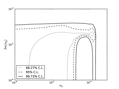
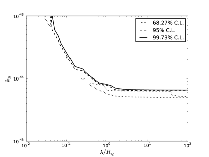
For the scalar long-range leptonic force, we find that after again fixing $m_{1,0}=0$, the best fit is at $k_{S}=6.73\times 10^{-45}$, $\lambda=1.56R_{\odot}$. Since $\lambda=1/m_{S}$, this point represents a force mediated by a scalar particle with mass $m_{S}=9.1\times 10^{-17}$eV and a coupling strength $g_{0}=2.91\times 10^{-22}$. The best fit survival probability is shown in the appendix in Fig. 31. Like the MaVaN case, the $pep$ survival probability is higher than ⁸B’s at the same energy. For the long-range vector force, we find the best fit at $k_{V}=3.26\times 10^{-54},\lambda=16.97R_{\odot}$, shown in Fig. 32. For the tensor long-range force, there is no improvement of the fit to the data and the best fit remains at MSW-LMA.

In all three cases, standard MSW-LMA is within the $1\sigma$ contour, but the constraint on the coupling strength gets stronger as $\lambda$ increases. The contours for the scalar case are shown in Fig. 25. At $\lambda=\infty$, we can set upper limits on the coupling strengths at 90% confidence level for 1 d.o.f. of

$$k_{S}(e) \leq 6.31\times 10^{-45}\text{ with }m_{1}=0\text{eV},$$ (40)

$$k_{V}(e) \leq 1.23\times 10^{-53},$$ (41)

$$k_{T}(e) \leq 1.31\times 10^{-61}\text{eV}^{-1}.$$ (42)

Figure 25: Results for MaVaN model with a scalar long-range force and $m_{1,0}=0$. Contours are shown for 68%, 95%, and 99.73% confidence levels (2 d.o.f.), where the $\chi^{2}$ has been minimized with respect to all undisplayed parameters.

IV.5 Non-Standard Solar Model

We found that using the low metallicity (AGSS09SF2) solar model’s flux constraints and solar distributions did not give noticeably different results, and in general worsened the fits for any model.

As described in Section III.4, we looked at the effect of changing the density of the solar core to see whether we are susceptible to mistaking a small difference in the expected solar model for a non-standard interaction. Fig. 26 shows the survival probability with the core density increased by various amounts. It is clear that within the range suggested by helioseismological measurements of about 1%, the change in the ⁸B upturn is not large enough to mimic any of the non-standard models. Fitting for the central density while keeping the rest of the fit the same, we find that the improvement in the fit for a change of up to 1% is marginal, and we don’t reach a minimum until an implausible increase in the solar core density of around 90%. Since any change in the central density would change the core temperature and thus also the expected fluxes, we fit again allowing the density to float and replacing the flux constraints from the solar model with an overall luminosity constraint and a constraint on the $pp$ to $pep$ ratio. Here the best fit is found at an increase of 57%, with a $\Delta\chi^{2}$ of $-4.6$, although not changing the density and just removing the flux constraints already gives a $\Delta\chi^{2}$ of -3.5.

Figure 26: (Color online) Survival probability for MSW-LMA with various fractional increases $\delta_{0}$ of the solar core density compared to the SNO results.

V Conclusions

We have compared the predictions of survival probabilities for several models of neutrino non-standard interactions compared to standard MSW-LMA oscillations using results from solar experiments constrained by terrestrial measurements of the mixing parameters. The results of the fits are summarized in Table 3.

Although several of these models allow for a better fit to the data and suggest an explanation for the flatness of the ⁸B survival probability, we have shown that with the current available data on solar neutrino interactions, there is no model that has demonstrated to be better than MSW-LMA with greater than $2\sigma$ significance. We have found that the low significance is in part due to the known, large value of $\theta_{13}$, but also because of the as-yet large systematic uncertainties and covariances in the experimental data sets. The critical transition region thus remains largely unexplored.

We have also examined whether small changes to the solar density profile could lead to a change in the transition region that could mimic the effects of new physics. The results of our simple model show that in fact this is not the case. The matter/vacuum transition region is therefore a good place to look for small effects of non-standard models.

Our best fit survival probabilities show that because most of our non-standard model effects have a solar radial or density dependence, the effect is lessened in the $pep$ or $pp$ production regions and so it would be difficult to test these models merely by improving the measurement of either of those signals. It would require either a better measurement of lower energy ⁸B, especially one with a charged-current interaction that preserves more of the spectral information, or a new model that can more closely match the data in order for this discrepancy to become more than a hint of something non-standard.

To fully probe this interesting region, in which the interferometry provided by neutrino oscillations lets us look for even tiny effects of new physics, will require new experiments or more precisely constrained systematic uncertainties. Both the Super-Kamiokande and Borexino experiments will continue to take data and hopefully their uncertainties will continue to improve. The SNO+ experiment will begin taking data in the near future and it, too, will be able to probe this region. It is possible, however, that a measurement using a charged-current reaction, which preserves more of the spectral information, may be necessary to provide the needed precision to see any new physics that may lie in this region.

Model	Best Fit	$\Delta\chi^{2}$	Additional D.o.F.	C.L.
MSW-LMA	$\Delta m^{2}_{21}=7.462\times 10^{-5}$ eV${}^{2},\sin^{2}\theta_{12}=0.301,$	0	—	—
	$\sin^{2}\theta_{13}=0.0242$
MSW-LMA (AGSS09SF2)	$\Delta m^{2}_{21}=7.469\times 10^{-5}$ eV${}^{2},\sin^{2}\theta_{12}=0.304,$	2.8	—	—
	$\sin^{2}\theta_{13}=0.0240$
NSI ($\epsilon_{1}$ real, $\epsilon_{2}=0$)	$\epsilon_{1}=-0.145$	-1.5	1	0.78
NSI ($\epsilon_{2}=0$)	$\epsilon_{1}=-0.146+0.031i$	-1.5	2	0.53
NSI ($\epsilon_{1}$ real)	$\epsilon_{1}=0.014$,$\epsilon_{2}=0.683$	-1.9	2	0.60
MaVaN neutrino density dependence	$m_{1,0}<0.033$ eV	0	1	0.0
MaVaN fermi density dependence	$\alpha_{2}=5.95\times 10^{-5},\alpha_{3}=i1.97\times 10^{-5}$	-3.4	2	0.81
Long range scalar leptonic force	$k_{S}=6.73\times 10^{-45},\lambda=1.56R_{\odot},m_{1,0}=0$eV	-2.9	3	0.58
Long range vector leptonic force	$k_{V}=3.26\times 10^{-54},\lambda=16.97R_{\odot}$	-1.8	2	0.59
Long range tensor leptonic force	$k_{T}<1.3\times 10^{-61}$eV-1	0	2	0.0
Non-standard solar model	$\delta_{0}=0.57$	-4.6	1	—
without flux constraint

Table 3: Comparison of survival probability fits to standard MSW-LMA. If the best fit remains at the MSW-LMA value for a model, a 90% confidence level upper limit (1 d.o.f.) on the model’s parameters is given instead. $\Delta\chi^{2}$ is the difference between the model’s best fit point and the MSW-LMA best fit. The final column gives the largest confidence level at which MSW-LMA is excluded.

*

Appendix A Survival Probability Fits

Figure 27: (Color online) Three flavor best fit NSI survival probability compared to MSW-LMA at $\epsilon_{1}=-0.145$, $\Delta m^{2}_{21}=7.481\times 10^{-5}$eV${}^{2},\sin^{2}\theta_{12}=0.320,\sin^{2}\theta_{13}=0.0238$. The top plot shows the survival probability as a function of incident neutrino energy. The middle shows the best fit’s predicted event rate in Borexino for each of Borexino’s measured electron energy bins scaled by the GS98SF2 flux no-oscillation prediction compared to Borexino’s data, and the bottom shows the same for S-K III’s energy bins and data.

Figure 28: (Color online) Best fit for NSI fit with $\epsilon_{2}=0$ but complex $\epsilon_{1}$ at $\epsilon_{1}=-0.146+0.31i$, $\Delta m^{2}_{21}=7.472\times 10^{-5}$eV${}^{2},\sin^{2}\theta_{12}=0.320,\sin^{2}\theta_{13}=0.0238$. The top plot shows the survival probability as a function of incident neutrino energy. The middle shows the best fit’s predicted event rate in Borexino for each of Borexino’s measured electron energy bins scaled by the GS98SF2 flux no-oscillation prediction compared to Borexino’s data, and the bottom shows the same for S-K III’s energy bins and data.

Figure 29: (Color online) Best fit for NSI fit with real $\epsilon_{1}$ at $\epsilon_{1}=0.014,\epsilon_{2}=0.683$, $\Delta m^{2}_{21}=7.487\times 10^{-5}$eV${}^{2},\sin^{2}\theta_{12}=0.310,\sin^{2}\theta_{13}=0.0238$. The top plot shows the survival probability as a function of incident neutrino energy. The middle shows the best fit’s predicted event rate in Borexino for each of Borexino’s measured electron energy bins scaled by the GS98SF2 flux no-oscillation prediction compared to Borexino’s data, and the bottom shows the same for S-K III’s energy bins and data.

Figure 30: (Color online) Best fit for fermion density dependent MaVaN at $\alpha_{2}=5.95\times 10^{-5},\alpha_{3}=i1.97\times 10^{-5}$, $\Delta m^{2}_{21}=7.484\times 10^{-5}$eV${}^{2},\sin^{2}\theta_{12}=0.320,\sin^{2}\theta_{13}=0.0239$. The top plot shows the survival probability as a function of incident neutrino energy. The middle shows the best fit’s predicted event rate in Borexino for each of Borexino’s measured electron energy bins scaled by the GS98SF2 flux no-oscillation prediction compared to Borexino’s data, and the bottom shows the same for S-K III’s energy bins and data.

Figure 31: (Color online) Best fit for scalar long-range force at $m_{1,0}=0$, $\lambda=1.56R_{\odot}$, $k_{S}=6.73\times 10^{-45}$, $\Delta m^{2}_{21}=7.484\times 10^{-5}$eV${}^{2},\sin^{2}\theta_{12}=0.320,\sin^{2}\theta_{13}=0.0239$. The top plot shows the survival probability as a function of incident neutrino energy. The middle shows the best fit’s predicted event rate in Borexino for each of Borexino’s measured electron energy bins scaled by the GS98SF2 flux no-oscillation prediction compared to Borexino’s data, and the bottom shows the same for S-K III’s energy bins and data.

Figure 32: (Color online) Best fit for vector long-range force at $\lambda=16.97R_{\odot}$, $k_{V}=3.26\times 10^{-54}$, $\Delta m^{2}_{21}=7.487\times 10^{-5}$eV${}^{2},\sin^{2}\theta_{12}=0.311,\sin^{2}\theta_{13}=0.0238$. The top plot shows the survival probability as a function of incident neutrino energy. The middle shows the best fit’s predicted event rate in Borexino for each of Borexino’s measured electron energy bins scaled by the GS98SF2 flux no-oscillation prediction compared to Borexino’s data, and the bottom shows the same for S-K III’s energy bins and data.