On the importance of nonlinear modeling in computer performance prediction

Abstract

Computers are nonlinear dynamical systems that exhibit complex and sometimes even chaotic behavior. The models used in the computer systems community, however, are linear. This paper is an exploration of that disconnect: when linear models are adequate for predicting computer performance and when they are not. Specifically, we build linear and nonlinear models of the processor load of an Intel i7-based computer as it executes a range of different programs. We then use those models to predict the processor loads forward in time and compare those forecasts to the true continuations of the time series.

1 Introduction

Accurate prediction is important in any number of applications. In a modern multi-core computer, for instance, an accurate forecast of processor load could be used by the operating system to balance the workload across the cores. The traditional models used in the computer systems community use linear, time-invariant (and often stochastic) methods, e.g., autoregressive moving average (ARMA), multiple linear regression, etc. [11]. While these models are widely accepted—and for the most part easy to construct—they cannot capture the nonlinear interactions that have recently been shown to play critical roles in a computer’s performance [4, 21]. As computers become more and more complex, these interactions are beginning to cause problems—e.g., hardware design “improvements” that do not work as expected. Awareness about this issue is growing in the computer systems community [20], but the modeling strategies used in that field have not yet caught up with those concerns.

An alternative approach that captures those complex effects is to model a computer as a nonlinear dynamical system [21, 22]—or as a collection of nonlinear dynamical systems, i.e., an iterated function system [1]. In this view, the register and memory contents are treated as state variables of these dynamical systems. The logic hardwired into the computer, combined with the code that is executing on that hardware, defines the system’s dynamics—that is, how its state variables change after each processor cycle. As described in previous IDA papers [2, 9], this framework lets us bring to bear the powerful machinery of nonlinear time-series analysis on the problem of modeling and predicting those dynamics. In particular, the technique called delay-coordinate embedding lets one reconstruct the state-space dynamics of the system from a time-series measurement of a single state variable. One can then build effective prediction models in this embedded space. One of the first uses of this approach was to predict the future path of a ball on a roulette wheel, as chronicled in [3] and revisited recently in [25]. Nonlinear modeling and forecasting methods that rely on delay-coordinate embedding have since been used to predict signals ranging from currency exchange rates to Bach fugues; see [6, 27] for good reviews.

This paper is a comparison of how well those two modeling approaches—linear and nonlinear—perform in a classic computer performance application: forecasting the processor loads on a CPU. We ran a variety of programs on an Intel i7-based machine, ranging from simple matrix operation loops to SPEC cpu2006 benchmarks. We measured various performance metrics during those runs: cache misses, processor loads, branch-prediction success, and so on. The experimental setup used to gather these data is described in Section 2. From each of the resulting time-series data sets, we built two models: a garden-variety linear one (multiple linear regression) and a basic nonlinear one: the “Lorenz method of analogues,” which is essentially nearest-neighbor prediction in the embedded state space [17]. Details on these modeling procedures are covered in Section 3. We evaluated each model by comparing its forecast to the true continuation of the associated time series; results of these experiments are covered in Section 4, along with some explanation about when and why these different models are differently effective. In Section 5, we discuss some future directions and conclude.

2 Experimental Methods

The testbed for these experiments was an HP Pavilion Elite computer with an Intel Core^® i7-2600 CPU running the 2.6.38-8 Linux kernel. This so-called “Nehalem” chip is representative of modern CPUs; it has eight cores running at 3.40Ghz and an 8192 kB cache. Its kernel software allows the user to monitor events on the chip, as well as to control which core executes each thread of computation. This provides a variety of interesting opportunities for model-based control. An effective prediction of the cache-miss rate of individual threads, for instance, could be used to preemptively migrate threads that are bogged down waiting for main memory to a lower-speed core, where they can spin their wheels without burning up a lot of power.

To build models of this system, we instrumented the kernel software to capture performance traces of various important internal events on the chip. These traces are recorded from the hardware performance monitors (HPMs), specialty registers that are built into most modern CPUs in order to log hardware event information. We used the libpfm4 library, via PAPI [5], to interrupt the executables periodically and read the contents of the HPMs. At the end of the run, this measurement infrastructure outputs the results in the form of a time series. In any experiment, one must be attentive to the possibility that the act of measurement perturbs the dynamics under study. For that reason, we varied the rate at which we interrupted the executables, compared the results, and used that comparison to establish a sample rate that produced a smooth measurement of the underlying system dynamics. A detailed explanation of the mechanics of this measurement process can be found in [2, 21, 22].

The dynamics of a running computer depend on both hardware and software. We ran experiments with four different C programs: two benchmarks from the SPEC cpu2006 benchmark suite (the 403.gcc compiler and the 482.sphinx speech recognition system) and two four-line programs (col_major and row_major ) that repeatedly initialize a matrix—in column-major and row-major order, respectively. These choices were intended to explore the range of current applications. The two SPEC benchmarks are complex pieces of code, while the simple loops are representative of repetitive numerical applications. 403.gcc works primarily with integers, while 482.sphinx is a floating-point benchmark. Row-major matrix initialization works naturally with modern cache design, whereas the memory accesses in the col_major loop are a serious challenge to that design, so we expected some major differences in the behavior of these two simple loops. Figure 1 shows traces of the instructions executed per cycle, as a function of time, during the execution of the two SPEC benchmarks on the computer described in the first paragraph of this section. There are clear patterns in the processor load during the operation of 482.sphinx . During the first 250 million instructions of this program’s execution, roughly two instructions are being carried out every cycle, on the average, by the Nehalem’s eight cores. Following that period, the processor loads oscillate, then stabilize at an average of one instruction per cycle for the period from 400-800 million instructions. Through the rest of the trace, the dynamics move between different regimes, each with characteristics that reflect how well the different code segments can be effectively executed across the cores. The processor load during the execution of 403.gcc , on the other hand, appears to be largely stochastic. This benchmark takes in and compiles a large number of small C files, which involves repeating a similar process, so the lack of clear regimes makes sense.

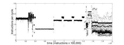
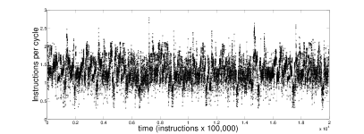
482.sphinx                                   403.gcc

Figure 1: Processor load traces of the programs studied here

The dynamics of row_major and col_major (not shown due to space constraints) were largely as expected. The computer cannot execute as many instructions during col_major because of the mismatch between its memory-access pattern and the design of the cache, so the baseline level of the col_major trace is much lower than row_major . Temporally, the row_major trace looks very much like 403.gcc : largely stochastic. col_major , on the other hand, has a square-wave pattern because of the periodic stalls that occur when it requests data that are not in the cache.

The following section describes the techniques that we use to build models of this time-series data.

3 Modeling computer performance data

3.1 Overview

The goal of this paper is to explore the effectiveness of linear and nonlinear models of computer performance. Many types of models, of both varieties, have been developed by the various communities that are interested in data analysis. We have chosen multiple linear regression models as our linear exemplar because that is the gold standard in the computer systems literature [20]. In order to keep the comparison as fair as possible, we chose the Lorenz method of analogues, which is the simplest of the many models used in the nonlinear time-series analysis community, as our nonlinear exemplar. In the remainder of this section, we give short overviews of each of these methods; Sections 3.2 and 3.3 present the details of the model-building processes.

3.1.1 Multiple Linear Regression Models

Suppose we have a set of $n$ observations from a system, where the $i^{th}$ observation includes $m+1$ measurements: a scalar response variable $r_{i}$ and a vector of $m$ explanatory variables $[e_{i1},\dots,e_{im}]$. Working from those $n$ observations $\{([e_{i1},\dots,e_{im}],r_{i})\}_{i=1}^{n}$, multiple linear regression (MLR) models the response variable via a linear combination of the explanatory variables—that is:

$$r_{i}=[1,e_{i1},...,e_{im}]\vec{\beta}$$ (1)

where $\vec{\beta}=[\beta_{1},\dots,\beta_{m+1}]^{T}$ is a vector of $m+1$ fit parameters [11, 15]. We estimated $\vec{\beta}$ by using ordinary least squares to minimize the sum of squared residuals (SSR) between the set of observations and the set of hyperplanes defined in equation (1):

$$SSR(\vec{\beta})=\sum_{i=1}^{n}(r_{i}-[1,e_{i1},...,e_{im}]\vec{\beta})^{2}=(\vec{r}-E\vec{\beta})^{T}(\vec{r}-E\vec{\beta})$$

Here, $E$ is a $n$ by $(m+1)$ matrix, with rows $\{[1,e_{i1},...,e_{im}]\}_{i=1}^{n}$. The $\vec{\beta}$ that minimizes this sum, $\hat{\beta}=(E^{T}E)^{-1}E^{T}\vec{r}$, is called the ordinary-least-squares estimator of $\vec{\beta}$ [15].

In practice, it is customary to measure everything that might be an explanatory variable and then use a method called stepwise backward elimination to reduce the model down to what is actually important. And in order to truly trust an MLR model, one must also verify that the data satisfy some important assumptions. These procedures are discussed in more detail in Section 3.2.

Advantages: MLR models are simple and easy to construct and use, as they only require a small vector-vector multiplication at each prediction step.

Disadvantages: strictly speaking, MLR can only be used to model a linear deterministic system that is measured without any error. MLR models involve multiple explanatory variables and cannot predict more than one step ahead.

3.1.2 Nonlinear Models

Delay-coordinate embedding [23, 24, 26] allows one to reconstruct a system’s full state-space dynamics from time-series data like traces in Figure 1. There are only a few requirements for this to work. The data, $x_{i}(t)$, must be evenly sampled in time ($t$) and both the underlying dynamics and the measurement function—the mapping from the unknown $d$-dimensional state vector $\vec{Y}$ to the scalar value $x_{i}$ that one is measuring—must be smooth and generic. When these conditions hold, the delay-coordinate map

$$F(\tau,d_{embed})(x_{i})=([x_{i}(t),\leavevmode\nobreak\ x_{i}(t+\tau),\leavevmode\nobreak\ \dots,\leavevmode\nobreak\ x_{i}(t+d_{embed}\tau)])$$ (2)

from a $d$-dimensional smooth compact manifold $M$ to $\mathbb{R}^{2d+1}$ is a diffeomorphism on $M$ [24, 26]: in other words, that the reconstructed dynamics and the true (hidden) dynamics have the same topology. This method has two free parameters, the delay $\tau$ and the embedding dimension $d_{embed}$, which must also meet some conditions for the theorems to hold, as described in Section 3.3. Informally, delay-coordinate embedding works because of the internal coupling in the system—e.g., the fact that the CPU cannot perform a computation until the values of its operands have been fetched from some level of the computer’s memory. This coupling causes changes in one state variable to percolate across other state variables in the system. Delay-coordinate embedding is designed to bring out those indirect effects explicitly and geometrically.

The mathematical similarity of the true and reconstructed dynamics is an extremely powerful result because it guarantees that $F$ is a good model of the system. As described on page 1, the nonlinear dynamics community has recognized and exploited the predictive potential of these models for some time. Lorenz’s method of analogues, for instance, is essentially nearest-neighbor prediction in the embedded space: given a point, one looks for its nearest neighbor and then uses that point’s future path as the forecast [17]. Since computers are deterministic dynamical systems [21], these methods are an effective way to predict their performance. That claim, which was first made in [9], was the catalyst for this paper—and the motivation for comparison of linear and nonlinear models that appears in the following sections.

Advantages: models based on delay-coordinate embeddings capture nonlinear dynamics and interactions, which the linear models ignore, and they can be used to predict forward in time to arbitrary horizons. They only require measurement of a single variable.

Disadvantages: these models are more difficult to construct, as estimating good values for their two free parameters can be quite challenging. The prediction process involves near-neighbor calculations, which are computationally expensive.

3.2 Building MLR forecast models for computer performance traces

In the experiments reported here, the response variable is the instructions per cycle (IPC) executed by the CPU. Following [20], we chose the following candidate explanatory variables (i) instructions retired (ii) total L2 cache misses (iii) number of branches taken (iv) total L2 instruction cache misses (v) total L2 instruction cache hits and (vi) total missed branch predictions. The first step in building an MLR model is to “reduce” this list: that is, to identify any explanatory variables—aka factors—that are meaningless or redundant. This is important because unnecessary factors can add noise, obscure important effects, and increase the runtime and memory demands of the modeling algorithm.

We employed the stepwise backward elimination method [7], with the threshold value (0.05) suggested in [11], to select meaningful factors. This technique starts with a “full model”—one that incorporates every possible factor—and then iterates the following steps:

1. If the $p$-value of any factor is higher than the threshold, remove the factor with the largest $p$-value

2. Refit the MLR model

3. If all $p$-values are less than the threshold, stop; otherwise go back to step 1

For all four of the traces studied here, this reduction algorithm converged to a model with three factors: L2 total cache misses, number of branches taken, and L2 instruction cache misses.

MLR models are meant to explain the value of the response variable in terms of the values of the explanatory variables, but they can also be used to predict it. To do this, one takes a measurement of each of the factors that appear in the reduced model (say, $[e_{1},\dots,e_{m}]$). One then makes a prediction of IPC by simply evaluating the function $[1,e_{1},\dots,e_{m}]\hat{\vec{\beta}}$ and assigning that response to the next time-step, i.e, $r_{t+1}$. That is how the predictions in the next section were constructed.

Like any model, MLR is technically only valid if the data meet certain conditions. Two of those conditions are not true for computer-performance traces: linear relationship between explanatory and response variables (which was disproved in [21]) and normal distribution of errors, which is clearly not the case in our data, given the nonlinear trends in residual quantile-quantile plots of our data (not shown). Despite this, MLR models are used routinely in the computer systems community [20]. And they actually work surprisingly well, as the results in Section 4 show.

3.3 Building nonlinear forecast models for computer performance traces

The first step in constructing a nonlinear forecast model of a time-series data set like the ones in Figure 1 is to perform a delay-coordinate embedding using equation (2). We followed standard procedures [12] to choose appropriate values for the embedding parameters: the first minimum of the mutual information curve [8] as an estimate of the delay $\tau$ and the false-nearest neighbors technique [14], with a threshold of 10-20%, to estimate the embedding dimension $d_{embed}$. For both traces in Figure 1, $\tau=100000$ instructions and $d_{embed}=12$. A plot of the reconstructed dynamics of these two traces appears in Figure 2.

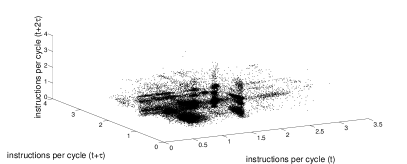
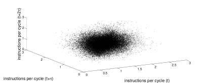
482.sphinx                                                      403.gcc 

Figure 2: 3D projections of delay-coordinate embeddings of the traces from Figure 1.

The coordinates of each point on these plots are differently delayed elements of the IPC time series: that is, IPC at time $t$ on the first axis, IPC at time $t+\tau$ on the second, IPC at time $t+2\tau$ on the third, and so on. An equivalent embedding (not shown here) of the row_major trace looks very like 403.gcc : a blob of points. The embedded col_major dynamics, on the other hand, looks like two blobs of points because of its square-wave pattern. Recall from Section 3.3 that these trajectories are guaranteed to have the same topology as the true underlying dynamics, provided that $\tau$ and $d_{embed}$ are chosen properly. And structure in these kinds of plots is an indication of determinism in that dynamics.

The nonlinear dynamics community has developed dozens of methods that use the structure of these embeddings to create forecasts of the dynamics; see [6, 27] for overviews. The Lorenz method of analogues (LMA) is one of the earliest and simplest of these strategies [17]. LMA creates a prediction of the future path of a point $\vec{x}_{o}$ through the embedded space by simply finding its nearest neighbor and then using that point’s future path as the forecast. The nearest neighbor step obviously makes this algorithm very sensitive to noise, especially in a nonlinear system. One way to mitigate that sensitivity is to find the $l$ nearest neighbors of $\vec{x}_{o}$ and average their future paths. These comparatively simplistic methods work surprisingly well for computer-performance prediction, as reported at IDA 2010 [9]. In the following section, we compare the prediction accuracy of LMA models with the MLR models of Section 3.2.

4 When and why are nonlinear models better at predicting computer performance?

4.1 Procedure

Using the methods described in Sections 3.2 and 3.3, respectively, we built and evaluated linear and nonlinear models of performance traces from the four programs described on page 2 (403.gcc , 482.sphinx , col_major and row_major ), running on the computer described in Section 2. The procedure was as follows. We held back the last $k$ points of each time series (referred to as “the test signal,” $c_{i}$). We then constructed the model with the remaining portion of the time series (“the learning signal”) and used the model to build a prediction $\hat{p}_{i}$. We computed the root mean squared prediction error between that prediction and the test signal in the usual way:

$$RMSE\leavevmode\nobreak\ =\sqrt{\frac{\sum_{i=1}^{k}(c_{i}-\hat{p_{i}})^{2}}{k}}$$

To compare the results across signals with different units, we normalized the RMSE as follows:

$$nRMSE\leavevmode\nobreak\ =\frac{RMSE\leavevmode\nobreak\ }{max\{c_{i}\}-min\{c_{i}\}}$$

The smaller the nRMSE , obviously, the more accurate the prediction.

4.2 Results and Discussion

First, we compared linear and nonlinear models of the two SPEC benchmark programs: the traces in the top row of Figure 1. For 403.gcc , the nonlinear LMA model was better than the linear MLR model (0.128 nRMSE versus 0.153). For 482.sphinx , the situation was reversed: 0.137 nRMSE for LMA and 0.116 for MLR. This was contrary to our expectations; we had anticipated that the LMA models would work better because their ability to capture both the gross and detailed structure of the trace would allow them to more effectively track the regimes in the 482.sphinx signal. Upon closer examination, however, it appears that those regimes overlap in the IPC range, which could negate that effectiveness. Moreover, this head-to-head comparison is not really fair. Recall that MLR models use multiple measurements of the system—in this case, L2 total cache misses, number of branches taken, and L2 instruction cache misses—while LMA models are constructed from a single measurement (here, IPC). In view of this, the fact that LMA beats MLR for 403.gcc and is not too far behind it for 482.sphinx is impressive, particularly given the complexity of these programs. Finally, we compared the linear and nonlinear model results to a simple “predict the mean” strategy, which produces a 0.140 and 0.250 nRMSE for 403.gcc and 482.sphinx , respectively—higher than either MLR or LMA.

In order to explore the relationship between code complexity and model performance, we then built and tested linear and nonlinear models of the row_major and col_major traces. The resulting nRMSE values for these programs, shown in the third and fourth row of Table 1, were lower than for 403.gcc and 482.sphinx , supporting the intuition that simpler code has easier-to-predict dynamics.

Program	Interrupt Rate (cycles)	LMA nRMSE	MLR nRMSE	naive nRMSE
403.gcc	100,000	0.128	0.153	0.140
482.sphinx	100,000	0.137	0.116	0.250
row_major	100,000	0.063	0.091	0.078
col_major	100,000	0.020	0.032	0.045
403.gcc	1,000,000	0.196	0.208	0.199
482.sphinx	1,000,000	0.137	0.187	0.462
row_major	1,000,000	0.057	0.129	0.103
col_major	1,000,000	0.028	0.305	0.312

Table 1: Normalized root-mean-squared error between true and predicted signals for linear (MLR), nonlinear (LMA), and “predict the mean” forecast strategies

Note that the nonlinear modeling strategy was more accurate than MLR for both of these simple four-line matrix initialization loops. The repetitive nature of these loops leaves its signature in their dynamics: structure that is exposed by the embedding process. LMA captures and uses that global structure—in effect, “learning” it—while MLR does not. Again, LMA’s success here is even more impressive in view of the fact that the linear models require more information to construct. Finally, note that the LMA models beat the naive strategy for both row_major and col_major , but the linear MLR model did not.

Another important issue in modeling is sample rate. We explored this by changing the sampling rate of the traces while keeping the overall length the same: i.e., by sampling the same runs of the same programs at 1,000,000 instruction intervals, rather than every 100,000 instructions. This affected the accuracy of the different models in different ways, depending on the trace involved. For 403.gcc , MLR was still better than LMA, but not by as much. For 482.sphinx , the previous result (MLR better than LMA) was reversed. For row_major and col_major , the previous relationship not only persisted, but strengthened. In both of these traces, predictions made from MLR models were less accurate than simply predicting the mean; LMA predictions were better than this naive strategy. See the bottom four rows of Table 1 for a side-by-side comparison of these results to the more sparsely sampled results described in the previous paragraphs.

To explore which model worked better as the prediction horizon was extended, we changed that value (the $k$ in Section 4.1) and plotted nRMSE . In three of the four traces—all but 482.sphinx —the nonlinear model held and even extended its advantage as the prediction horizon lengthened; see Figure 3 for some representative plots.

Figure 3: nRMSE versus prediction horizon.Top: col_major Bottom: 482.sphinx 

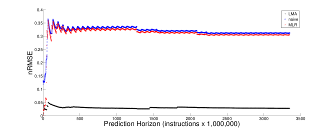
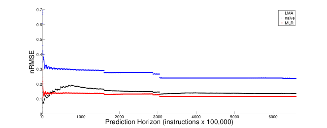
The initial variability in these plots is an artifact of normalizing over short signal lengths and should be disregarded. The vertical discontinuities (e.g., at the 1300 and 2100 marks on the horizontal axis of the col_major plot, as well as the 1600 and 3000 marks of 482.sphinx ) are also normalization artifacts. The sawtooth pattern in the top two traces in col_major nRMSE are due to the cyclical nature of that loop’s dynamics. LMA captures this structure, while MLR and the naive strategy do not, and thus produces a far better prediction.

5 Conclusion

The experiments reported in this paper indicate that even a very basic nonlinear model is generally more accurate than the state-of-the-art linear model in the computer performance literature. This result is even more striking because those linear models require far more information to build than the nonlinear models do—and they cannot be used to predict further than one timestep into the future. It is somewhat surprising that these linear models work at all, actually, since many of the assumptions upon which they rest are not satisfied in computer performance applications. Nonlinear models that work in delay-coordinate embedding space may be somewhat harder to construct, but they capture the structure of the dynamics in a truly effective way.

It would be of obvious interest to apply some of the better linear models that have been developed by the data analysis and modeling communities to the problem of computer performance prediction. Even a segmented or piecewise version of multiple linear regression [16, 19], for instance, would likely do a better job at handling the nonlinearity of the underlying system. The difficulty with that approach, of course, is how to choose the breakpoints between the segments. And MLR is not really designed to be a temporal predictor anyway; linear predictors like the ones presented in [18] might be much more effective. There are also regression-based nonlinear models that we could use, such as [10], as well as the many other more-sophisticated models in the nonlinear dynamics literature [6, 27]. It might be useful to develop nonlinear models that use sliding windows in the data in order to adapt to regime shifts, but the choice of window size is an obvious issue. Finally, nonlinear models that use multiple probes—like MLR does—could be extremely useful, but the underlying mathematics for that has not yet been developed.

References

- [1] Alexander, Z., Bradley, E., Garland, J., Meiss, J.: Iterated function system models in data analysis: Detection and separation. CHAOS 22(2) (April 2012)
- [2] Alexander, Z., Mytkowicz, T., Diwan, A., Bradley, E.: Measurement and dynamical analysis of computer performance data. In: Adams, N., Berthold, M., Cohen, P. (eds.) Advances in Intelligent Data Analysis IX, vol. 6065. Springer Lecture Notes in Computer Science (2010)
- [3] Bass, T.: The Eudaemonic Pie. Penguin, New York (1992)
- [4] Berry, H., Perez, D., Temam, O.: Chaos in computer performance. Chaos 16 (2006)
- [5] Browne, S., Deane, C., Ho, G., Mucci, P.: PAPI: A portable interface to hardware performance counters. In: Proceedings of Department of Defense HPCMP Users Group Conference (1999)
- [6] Casdagli, M., Eubank, S. (eds.): Nonlinear Modeling and Forecasting. Addison Wesley (1992)
- [7] Faraway, J.J.: Practical regression and anova using r (2002)
- [8] Fraser, A., Swinney, H.: Independent coordinates for strange attractors from mutual information. Physical Review A 33(2), 1134–1140 (1986)
- [9] Garland, J., Bradley, E.: Predicting computer performance dynamics. In: Proceedings of the 10th international conference on Advances in intelligent data analysis X. pp. 173–184. IDA’11, Springer-Verlag, Berlin, Heidelberg (2011)
- [10] Grassberger, P., Hegger, R., Kantz, H., Schaffrath, C., Schreiber, T.: On noise reduction methods for chaotic data. Chaos 3, 127 (1993)
- [11] Jain, R.: The Art of Computer Systems Performance Analysis: Techniques for Experimental Design, Measurement, Simulation, and Modeling. John Wiley & Sons, 2nd edn. (1991)
- [12] Kantz, H., Schreiber, T.: Nonlinear Time Series Analysis. Cambridge University Press, Cambridge (1997)
- [13] Kennel, M., Isabelle, S.: Method to distinguish possible chaos from colored noise and to determine embedding parameters. Phys. Rev. A 46, 3111 (1992)
- [14] Kennel, M.B., Brown, R., Abarbanel, H.D.I.: Determining minimum embedding dimension using a geometrical construction. Physical Review A 45, 3403–3411 (1992)
- [15] Legendre, A.: Nouvelles méthodes pour la détermination des orbites des comètes. F. Didot (1805)
- [16] Liu, J., Wu, S., Zidek, J.: On segmented multivariate regression. Statistica Sinica 7, 497–525 (1997)
- [17] Lorenz, E.N.: Atmospheric predictability as revealed by naturally occurring analogues. Journal of the Atmospheric Sciences 26, 636–646 (1969)
- [18] Makhoul, J.: Linear prediction: A tutorial review. Proceedings of the IEEE 63(4), 561–580 (1975)
- [19] McZgee, V.E., Carleton, W.T.: Piecewise regression. Journal of the American Statistical Association 65(331), 1109–1124 (1970)
- [20] Moseley, T., Kihm, J.L., Connors, D.A., Grunwald, D.: Methods for modeling resource contention on simultaneous multithreading processors. In: Proceedings of the 2005 International Conference on Computer Design (ICCD) (October 2005)
- [21] Myktowicz, T., Diwan, A., Bradley, E.: Computers are dynamical systems. Chaos 19, 033124 (2009), doi:10.1063/1.3187791
- [22] Mytkowicz, T.: Supporting experiments in computer systems research. Ph.D. thesis, University of Colorado (November 2010)
- [23] Packard, N., Crutchfield, J., Farmer, J., Shaw, R.: Geometry from a time series. Physical Review Letters 45, 712 (1980)
- [24] Sauer, T., Yorke, J., Casdagli, M.: Embedology. Journal of Statistical Physics 65, 579–616 (1991)
- [25] Small, M., Tse, C.: Predicting the outcome of roulette. CHAOS 22, 033150 (2012)
- [26] Takens, F.: Detecting strange attractors in fluid turbulence. In: Rand, D., Young, L.S. (eds.) Dynamical Systems and Turbulence, pp. 366–381. Springer, Berlin (1981)
- [27] Weigend, A., Gershenfeld, N. (eds.): Time Series Prediction: Forecasting the Future and Understanding the Past. Santa Fe Institute Studies in the Sciences of Complexity, Santa Fe, NM (1993)