∎
33institutetext: CMAP, Ecole Polytechnique, 33email: caroline.hillairet@polytechnique.edu 44institutetext: This research benefited from the support of the Chaires “Dérivés du Futur” and “Finance et Développement durable”.
55institutetext: Université Paris-Est, CERMICS (ENPC), INRIA, 55email: jourdain@cermics.enpc.fr 66institutetext: This research benefited from the support of the Eurostars E!5144-TFM project and of the Chaire “Risques Financiers“, Fondation du risque.
77institutetext: IMT Université Paul Sabatier, 77email: pontier@math.univ-toulouse.fr
Reducing the debt: Is it optimal to outsource an investment?
Abstract
This paper deals with the problem of outsourcing the debt for a big investment, according two situations: either the firm outsources both the investment (and the associated debt) and the exploitation to another firm (for example a private consortium), or the firm supports the debt and the investment but outsources the exploitation. We prove the existence of Stackelberg and Nash equilibria between the firms, in both situations. We compare the benefits of these contracts, theorically and numerically. We conclude with a study of what happens in case of incomplete information, in the sense that the risk aversion coefficient of each partner may be unknown by the other partner.
Keywords:
Outsourcing, Public Debt, Public-Private-Partnership, Nash and Stackelberg equilibria, Optimization, Partial informationMSC 2010: 60H30, 91B06, 91B50, 93E20
JEL: C62, C62, G28, H63.
1 Introduction
With the significant increase in recent years of public debt in many developed countries, together with the associated concerns related to possible defaults of some of them, the question of financing public projects is more than ever at the center of economic and political considerations. To overcome this problem, leveraging on the private sector appears at first glance as a good idea. This type of Public-Private Partnership (PPP) was initiated in the United Kingdom in 1992, under the name Private Financing Initiative (PFI), and has widely been used since then, so that it represented one third of all public investments made in the UK during the period 2001-2006. It has also been used in many other countries, in particular in Europe, Canada and in the United States, to finance hospitals, prisons or stadiums among others. It is also recommended by the OECD. We refer among many other references to EFG for an overview of the extent of PPPs in Europe and in the US, to the website of the European PPP Expertise Center (EPEC) or the website of the National Council for Public-Private Partnerships, and to OECD for a global overview made by the OECD.
However, as emphasized by the recent discussions in the UK, although the benefits of this type of partnership are mainly admitted, there are still many concerns about its drawbacks (see WBI for a detailed overview). Even though some drawbacks are of political, social or behavioral natures, others are purely economic and are the ones that we are interested in. More precisely, we would like to answer the following question: from an economic point of view, and taking into account the constraints that a country faces when issuing a new amount of debt, is it optimal for this country to finance a public project via a private investment?
Although already of a big interest, this question does not need to be restricted to debt issuance by a country but can be generalized to any economic agent, be it a country or a firm. Indeed, any firm has some constraints on its debt level for several reasons. In some cases, banks will simply not allow a company to borrow enough money to sustain a very expensive project. But even if it is not the case, since the debt level appears on the company’s accounts, issuing too much debt will affect the opinion and confidence of investors, and in particular deteriorate its rating. This can lead to a higher credit spread when issuing new bonds, difficulties to increase the capital of the firm, a drop of the company’s stock price, dissatisfaction of shareholders or in the worst case, bankruptcy. We can cite some concrete examples where the dilemma between investing directly or resorting to outside investment can occur: owning or renting offices or factories, owning or leasing trucks, trains or planes, some industrial machines or some office materials (such as computers).
Therefore we will consider in this paper the problem of outsourcing from the debt point of view. Since the question of outsourcing some operations has already been widely studied and our aim is only to study the relevance of outsourcing an investment in order to reduce the debt of a firm (or economic agent), we will compare two situations where the operations are always outsourced. In the first one, the firm outsources both the investment/debt and the operations, while in the second one, the firm supports the debt and the investment but outsources the operations. In both situations, the investment is covered by issuing a debt at time 0 but the cost of borrowing of the outsourcer and the outsourcee may be different. More specifically, we suppose that the outsourcer faces some important constraints if he has to issue a new debt, stylized by a convex function modeling his aversion for debt issuance. That is why he considers the possibility to outsourcing the investment to a firm which has less constraints.
In IMP, Iossa, Martimort and Pouyet give some results on the comparison of the costs and benefits associated to PPP. Hillairet and Pontier CaroMo propose a study on PPP and their relevance, assuming the eventuality of a default of the counterparty, but they do not take into account the government debt aversion. However, the attractivity for government of PPP contracts relies obviously on the short term opportunity gain to record infrastructure assets out of the government’s book. To our knowledge, there does not exist any reference in Mathematics area. In Economics, a narrow strand of literature is dedicated to the discussion of Build-Operate-Transfer (BOT) concession contracts, which is a frequent form of PPP. Under BOT contracts the private sector builds and operates an infrastructure project for a well defined concession period and then transfers it to public authorities. The attractiveness of BOT contracts to governments stems from the possibility to limit governmental spending by shifting the investment costs to a private consortium. In AuPi1, Auriol and Picard discuss the choice of BOT contracts when governments and consortia do not share the same information about the cost parameter during the project life. They summarize the government’s financial constraint by its “shadow” cost of public funds, which reflects the macro-economic constraints that are imposed on national governments’ surplues and debt levels by supranational institutions such as the I.M.F. Using linear demand functions and uniform cost distributions, they compute theoretical values of shadow costs that would entice governments to choose BOT concessions contracts. Our approach is different from the modelization and the resolution point of view.
This paper studies, in a two-period setting, two kinds of equilibria between risk averse firms. The first one is a Stackelberg equilibrium with the outsourcer as leader, which corresponds to the more classic setting for outsourcing situations. The second one is a Nash equilibrium. It may correspond to an outsourcing between two economic entities within a same group: in this case, the two entities make their decisions simultaneously and a Nash equilibrium is more favourable for the group than a Stackelberg one. For both situations where the investment is outsourced or not, Stackelberg and Nash equilibria are characterized. A theorical comparison is provided for the Nash equilibrium, from the point of view of the outsourcer: we check that the investment should be outsourced if the outsourcee has a lower cost of capital or if the outsourcer has a high debt aversion. For the Stackelberg equilibrium, the comparison is done numerically on a concrete example. The analysis is extended to an incomplete information setting in which the firms do not have perfect knowledge of the preference of their counterparty. To model the social need of the investment, the outsourcer gets a penalty if the outsourcee does not accept the contract.
The present paper is organised as follows. In Section 2 we set the problem of outsourcing between two firms and we define the optimization problems in Situation 1, in which the firm outsources both the investment/debt and the operations, and in Situation 2 , in which the firm supports the debt and the investment but outsources the operations. Section 3 provides the main results concerning Nash and Stackelberg equilibria, the comparison between the two situations, and the case of incomplete information. The proofs are postponed in Appendices. We provide in Section 4 a numerical example to better investigate the quantitative effects of the model. Appendix 5 is devoted to the proofs of existence and characterization of Nash and Stackelberg equilibria in Situation 1, then Appendix LABEL:sec:proof2 does the same in Situation 2. Appendix LABEL:sec:proof3 concerns the proofs of the comparison results between the two situations and Appendix LABEL:proofIncInf the results obtained in incomplete information.
2 Problem formulation
2.1 Costs and revenue
Consider two firms. Firm is the one who wants to reduce its debt and therefore considers the possibility of outsourcing an investment to a second firm . In any case, firm is the one that will support the operational cost of the project, on the time horizon . Let the operational cost on the time-interval be given by:
| (1) |
where
-
•
is the “business as usual” cost, such that represents the “average” benchmark cost (it takes into account the price of commodities, employees, rents…). We assume that is a non constant random variable bounded from below by a finite constant on a probability space such that
(2) Notice that this implies that the function is infinitely differentiable.
-
•
is a non-negative parameter and represents the effort made on the time-interval in order to reduce the operational cost such as logistics improvements, research and development, maintenance or more efficient or less workers. will in general have a social impact for firm ,
-
•
represents the impact of the quality of the investment on the reduction of operational costs. We do not impose any restriction on the sign of since, as suggested in IMP, both signs can make sense depending on the situation. Indeed, when constructing a building, using more expensive material usually brings less maintenance costs and therefore a positive delta. On the contrary, for a hospital, using more sophisticated (and expensive) machines can bring bigger maintenance costs and a negative delta.
-
•
is the effort done at time to improve the (initial) quality of the investment, improving in the meantime the social value of the project. Depending on , affects positively, negatively or does not affect the operational cost. Remark is that has the same dimension as the effort ,
-
•
and , modeling the respective impacts of the efforts and respectively on the operational cost , are , increasing and strictly concave functions, satisfying the Inada conditions and , and . We also assume that where is the lower bound of the random variable and , which ensures that ; as a consequence, We assume furthermore that for for technical reasons and to make the computations lighter even if we could relax this last assumption.
The parameter is a control for firm , while is a control for the firm that supports the investment, or depending on the situation; represents the cost on the time-interval .
The minimal investment required by the project is and if initial effort are done (i.e. if ) the total investment is the sum . This investment is assumed to be entirely covered by issuing a debt with horizon at time . To take into account the possibility that the cost of borrowing is in general not the same for different firms, we denote the respective non-negative constant interest rates of firms and by and .
On the time-interval , the amount to be reimbursed by the borrower is .
Finally, we need to add the remaining costs on coming from the effort as well as the maintenance costs denoted by :
| (3) |
The maintenance cost is a non-negative parameter and will have a social impact for firm .
Since firm gives to firm either a rent or the right to exploit the project on , in both cases we can consider a random variable which corresponds to the endowment for firm and the rent or shortfall for firm , on . This variable is computed using a reasonably simple rule, decided at and subject to a control of firm . In reality, in such contracts, the endowment can be indexed on the price of commodities in the case of transportation or on a real-estate index for the rent of a building. Since firm wants to have a project of good quality as well as a well maintained project, we assume that is a non-negative random variable and depends on both and the maintenance cost in the following way:
| (4) |
with , , and is a , increasing and strictly concave function on , such that and . Moreover, we assume that
| (5) |
The constants , and are controls of firm . We do not put any randomness in the coefficients , and of since we consider that they are defined at time by a contract between firms and . All the randomness in comes from the operational cost term . Still, this model allows for an indexation on a benchmark such as the price of commodities or inflation through this dependence on operational costs.
2.2 Optimization problems
We assume that the risk aversions of firm and are represented respectively by the
exponential utility functions and , ,
with .
We consider two different situations: in Situation 1, firm supports the debt and
takes care of the exploitation; its controls are , and , whereas the controls
of firm are , and . In Situation 2, firm only takes care
of the exploitation, its controls are and , whereas the controls of firm are
, , and . Firm is the one that chooses between the two situations. The optimization problems for firm respectively in Situation 1 and 2
are and respectively, where:
| (6) | |||||
| (7) |
recalling .
In these optimization problems, we have assumed that the controls of firm are given (they have no reason to be the same in the two cases). We look for controls in the following admissible sets: and are non-negative constants. The eventuality that firm does not accept the contract will be taken into account in the constraints of the optimization problem for firm .
On the other hand, we consider that the project has an initial “social” value for firm , and a good maintenance also represents a social benefit . The benefits of the efforts on operational costs are modelled through the function . We also introduce a penalization function representing the aversion for debt issuance of firm (firm has no debt aversion). Those functions satisfy the following hypotheses
-
•
is a , increasing and concave function. , possibly infinite, and .
-
•
is a , increasing and concave function, such that and .
-
•
is a , increasing and concave function, such that and
-
•
is an increasing and strictly convex function, satisfying .
Therefore we write the optimization problem for firm in both situations as and where:
Hypotheses on and imply that
is strictly concave, satisfies and .
Finally we assume that , possibly infinite.
The admissible sets are:
- in Situation 1, , , and such that
| (8) |
- in Situation 2, , , , and such that
| (9) |
The constraint ensures that firm will accept the contract, since it is better or equal for it than doing nothing.
The most natural equilibrium to be considered in outsourcing situations is a Stackelberg equibrium with firm as leader. It corresponds for example to a government which outsources the construction of a stadium, or to an industrial group which wants to outsource its trucks/trains to a transport company. Nevertheless, within a group, a given entity may be interested in outsourcing its debt to another entity of the same group. In this situation, a Nash equilibrium is more relevant. Therefore this paper addresses those two kinds of equilibria.
Remark 1
A Stackelberg equilibrium with firm leader is never relevant from an economical perspective, since it is never the outsourcee who makes an offer to the outsourcer. It is also not interesting from a mathematical point of view. Indeed, in Situation , since , is decreasing with respect to , while is increasing with respect to . Therefore if firm is the leader, for any choice of its controls, firm ’s optimal controls will always bind the constraint .
3 Main results
The best responses of firm to given controls of firm turn out to be easily derived. That is why we first present them, before stating our main results concerning Nash and Stackelberg equilibria where these best responses appear. The proofs of the main results are postponed in Appendices 5, LABEL:sec:proof2, LABEL:sec:proof3, LABEL:proofIncInf.
3.1 Best responses of firm in Situations and
Let us first consider Situation and suppose that is given in . For firm the optimization problem is by , and since is increasing it writes:
Since , and are strictly concave, the first order conditions characterize the points maximizing each function between braces and, with the convention that for , we have :
| (10) |
Let us now consider Situation and suppose that is given. Similarly we obtain that
| (11) |
When useful to explicit the dependence of these best responses of firm with respect to the controls of firm , we use the notation , and .
To describe the Nash and Stackelberg equilibria, we introduce the continuous mapping , and defined by
| (12) | |||||
| (13) | |||||
| (14) |
3.2 Nash equilibria
To describe the Nash equilibria, we need the following technical result about the function :
Lemma 1
The function is continuous, satisfies and is decreasing from to on (where is defined in (5)) and increasing from to on thus admitting an continuous inverse .
Theorem 3.1
Remark 2
-
•
Although there exists an infinite number of Nash equilibria, the controls , and are the same in all these equilibria.
-
•
Since , one has so that
. -
•
It is natural to wonder whether there exists in Situation 1 a Nash equilibrium among the infinite family of such equilibria exhibited in Theorem 3.1 which maximizes . This function depends on the Nash equilibrium only through the term which has to be maximized. The function being concave, it admits a unique maximum on the interval where associated with a Nash equilibrium varies. When (which is the case for the numerical example investigated in Section 4), then and the optimal value of will turn out to be the optimal control in the Stackelberg equilibria (see Theorems 3.5 and 3.6 below).
Otherwise, .
Theorem 3.2
Let . In Situation 2, there exists an infinite number of Nash equilibria namely the vectors defined by
| (17) | |||||
| (18) | |||||
| (19) |
and such that , a condition that is satisfied when .
Moreover, and if , then is positive and unique for each .
The corresponding optimal values for firms and are respectively and
Let denote the set of for which there exists such that is a Nash equilibrium in Situation 2.
Remark 3
-
•
Notice that the order the different controls are determined is important, since some of them depend on the other ones. Indeed depends on no other control and therefore should be determined first, leading to the value of . Then one should fix , in order to have , which allows then to determine , and once this is done, we can find . Although and essentially play the same role, the fact that only depends on makes this order important. If one chooses first, then the determination of is not clear, since then depends on , while depends on and .
-
•
We expect that, as in Situation 1, when (which is the case for the numerical example investigated in Section 4), then . Indeed, a formal differentiation of with respect to leads to since, because of the first order optimality condition related to (18), one should not need to take care of the dependence of on . Moreover, one easily checks that the unique solution to is . This is illustrated in Figure 1.
We now compare the respective optimal values and for firm in Situations and for the same maintenance effort . According to Remarks 2 and 3, the same value is likely to maximize and . Therefore choosing the same maintenance effort for the comparison is natural. Notice also that, by Theorem 3.2 and Remark 2, . Let (resp. ) denote the value of the control in the Nash equilibrium with in Situation 1 (resp. in Situation 2 when ).
We are going to exhibit cases in which Situation 1 (meaning outsourcing (respectively Situation 2, meaning debt issuance) is the more profitable for firm I.
Theorem 3.3
Let rate be fixed and . In case of rate satisfying
| (20) |
we have and the better contract for firm is the second one, meaning debt issuance.
Condition (20) has a clear economical interpretation. The right-hand side does not depend on . Therefore for a fixed , debt issuance is the best choice for firm as soon as its interest rate is small enough. Note the impact of the function modeling its debt aversion : the larger , the smaller the threshold on in condition (20), look at Figure 2.
Theorem 3.4
We assume Let rate be fixed (thus is fixed) and . In case of rate satisfying
| (21) |
and one of the following:
| or | ||||
one has and the better contract for firm is the first one, meaning outsourcing.
The economical interpretation of condition (3.4) is natural. Indeed, the right-hand sides of the inequalities do not depend on whereas the left-hand sides are increasing functions of . Hence (3.4), leading to optimality of outsourcing for firm , is satisfied as soon as its interest rate is large enough. Besides, we see that the more convex is, the smaller is the threshold on in the first inequality of condition (3.4).
3.3 Stackelberg equilibria
Depending on Situation 1 or 2 and on the sign of , the optimal will be characterized as solution of different equations. To specify those equations, we need to introduce the functions
| (23) |
| (24) |
| (25) |
where is a positive function of defined as follows,
| (26) |
We consider the following equations
| (27) |
| (28) |
| (29) |
Theorem 3.5
In Situation 1, there exists at least one Stackelberg equilibrium with firm as the leader. Moreover, if there exists a Stackelberg equilibrium with , then it is characterized by :
If then
is a solution of (28) and is less than .
If then either is less than and solves (27) or is larger than one and solves (29).
The corresponding optimal values for firms and are respectively and .
Theorem 3.6
In Situation 2, there exists at least one Stackelberg equilibrium with firm as the leader.
Moreover, if there exists a Stackelberg equilibrium
with , then it satisfies:
is a solution of (27), , , ,
and
,
where the mappings and are defined by (12)-(14).
In particular, .
Moreover, if , then is a singleton and .
The corresponding optimal values for firms and are respectively and .
Proposition LABEL:eq5.5 below states that Equation (27) which appears in the characterization of when in both Situations 1 and 2 always admits a solution.
An analytical comparison is not so easy, but Figures 4 and 5 allow a numerical comparison between debt issuance and outsourcing.
3.4 Incomplete information
In this section we consider the previous equilibrium problems when the firms do not have a perfect knowledge of the preferences of the other firm. More precisely, we still assume that the firms’ utility functions are and respectively, but firm perceives as a -valued random variable with known distribution and independent from that we denote and firm perceives as a random variable with known distribution and independent from that we denote . According to Section (3.1), firm optimal controls are functions of the controls fixed by firm that do not depend on the risk aversion parameters . Therefore, equations (10) and (11) still hold in incomplete information and incomplete information on the risk aversion parameter has no impact on the equilibria. In contrast, the uncertainty on the parameter has an impact as the acceptation of the contract by firm depends on it. To model the social need of the investment, we introduce a (social) penalty that firm gets if firm does not accept the contract.
3.4.1 Stackelberg equilibrium, firm is leader
We first introduce
the events “firm accepts the contract” in Situation .
The optimization problem for firm is
| (30) |
in Situation 1 and in Situation 2, it becomes :
| (31) |
The functions
where and have been defined in (10),
are the social gain that firm respectively gets in Situations and if firm accepts the contract. Notice that the supremum is taken with to model the possibility for firm not to enter the game and that corresponds to the case where firm absolutely wants that firm accepts the contract.
In order to characterize the acceptance set , we introduce
| (32) |
and
| (33) |
Firm accepts the contract if and only if , thus .
We define the value function of the problem with complete information that firm ’s risk aversion is equal to
These value functions are respectively obtained for the Stackelbreg equilibria given in Theorems 3.5 and 3.6. We have the following result:
Theorem 3.7
Let
| (34) |
We have and when either or then .
Theorem 3.7 has an important interpretation. Indeed, it means that in order to solve (30) or (31), firm first solves its problem for any given as if the information was complete or in other words as in Section 3.3, and then ”chooses” the level that would bring the greatest social expectation in (34).
Theorem 3.8
Let . If then the fact
that the two firms do not enter into any contract is a Stackelberg equilibrium in Situation .
Otherwise, if then the optimization problem
(34) has a solution (equal to when ) and any Stackelberg equilibrium for the problem with complete information and risk aversion for firm is a Stackelberg equilibrium for the problem with incomplete information.
3.4.2 Nash equilibrium
We did not succeed in finding sufficient conditions for the existence of a Nash equilibrium with incomplete information. Nevertheless, we obtain necessary conditions that are similar for both situations:
Theorem 3.9
Assume existence of a Nash equilibrium such that the value for firm is greater than and let with defined (using ) in Situations 1 and 2 respectively as
Then ,
and in Situation 1,
.
If , then is a Nash equilibrium for the problem with complete information and risk aversion for firm and for each , .
If , then for each , .
Remark 4
If there is a vector of elements of such that
, one deduces that if there exists a Nash equilibrium for the problem with incomplete information, then such that .
4 Numerical Example
We investigate a numerical example to better quantify and compare the two different situations (Situation 1: outsourcing, Situation 2 : debt issuance) and the two equilibria (Nash and Stackelberg equilibria). We have chosen the following numerical values:
-
•
the risk aversion parameters are ,
-
•
the impact of the quality of the investment on the operational costs is ,
-
•
the minimal investment is ,
-
•
the random cost follows a uniform distribution on the interval , with and ,
-
•
the aversion to debt issuance is (or ),
-
•
the benefits functions are and ,
-
•
the impact of the maintenance cost on the rent is modeled by the function , and the impact of the efforts and on the operational costs by the functions (thus satisfying the condition ),
-
•
the interest rates and over the period (when borrowing initially, firm has to reimburse on the time-interval ) vary in the interval .
4.1 Nash equilibrium
Dependency on the maintenance costs in Nash equilibrium
We now investigate the Nash equilibria in both situations. As stated in Theorem 3.1 and Theorem 3.2, the optimal value functions and depend on the optimal maintenance costs . Figure 1 gives an insight of this dependency, for two different values of in Situation 1 and for a larger value of in Situation 2. We notice that outsourcing is worthless for average maintenance costs (between and of for ) We also observe that the smaller , the larger is the interval of values for which outsourcing is better than debt issuance.
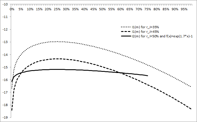
The maintenance costs numerically optimizing the value functions and is (which is also the maintenance costs in Stackelberg equilibrium, whatever the situation) as expected from Remarks 2 and 3. Therefore, in the forthcoming figures, the Nash equilibrium is computed for this optimal maintenance costs .
Dependency on the interest rates and in Nash equilibrium
Figure 2 gives, for Nash equilibrium, the optimal value function in Situation 1 (outsourcing) as a function of , and in Situation 2 (debt issuance) as a function of and for two differents functions of debt aversion ( or ).
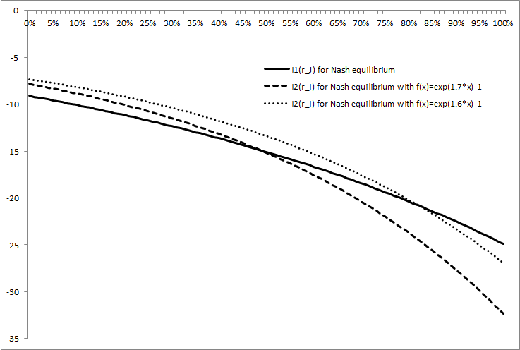
We notice that the greater the debt aversion function , the smaller the value of at which it becomes more favourable to outsource ( for , for ).
Outsourcing or not in Nash equilibrium?
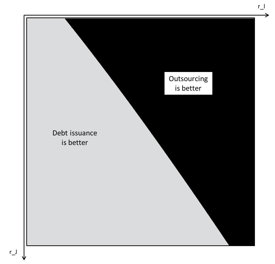
Figure 3 gives a decision criterion of outsourcing or not, function of in the -axis and in the -axis. The grey area corresponds to the region where it is optimal to issue debt, while the black area corresponds to the region where it is optimal to outsource. As expected, if it is optimal to outsource for a given couple , then it remains optimal to outsource for all couples with . If it is optimal to issue debt for a given couple , then it remains optimal to issue debt for all couples with .
4.2 Stackelberg equilibrium
Dependency on the interest rates and in Stackelberg equilibrium
Figure 4 below gives, for Stackelberg equilibrium, the optimal value function in Situation 1 (outsourcing) as a function of , and in Situation 2 (debt issuance) as a function of and for two different functions of debt aversion ( or ).
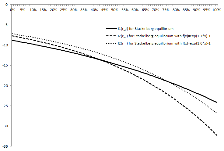
The conclusions are the same as the ones in Figure 2 for Nash equilibrium, and we notice that the value functions and are slightly greater in Stackelberg equilibrium than in Nash equilibrium. Moreover, the range of interest rate for which outsourcing is more favourable is slightly wider in Stackelberg equilibrium than in Nash equilibrium ( for , for ). Indeed, being a leader in Stackelberg equilibrium, firm has a more favourable position to get better conditions to outsource, in comparison with Nash equilibrium.
Outsourcing or not in Stackelberg equilibrium?
Figure 5 gives a decision criteria of outsourcing or not, function of in the -axis and in the -axis. The grey area corresponds to the region where it is optimal to issue debt, while the black area corresponds to the region where it is optimal to outsource.
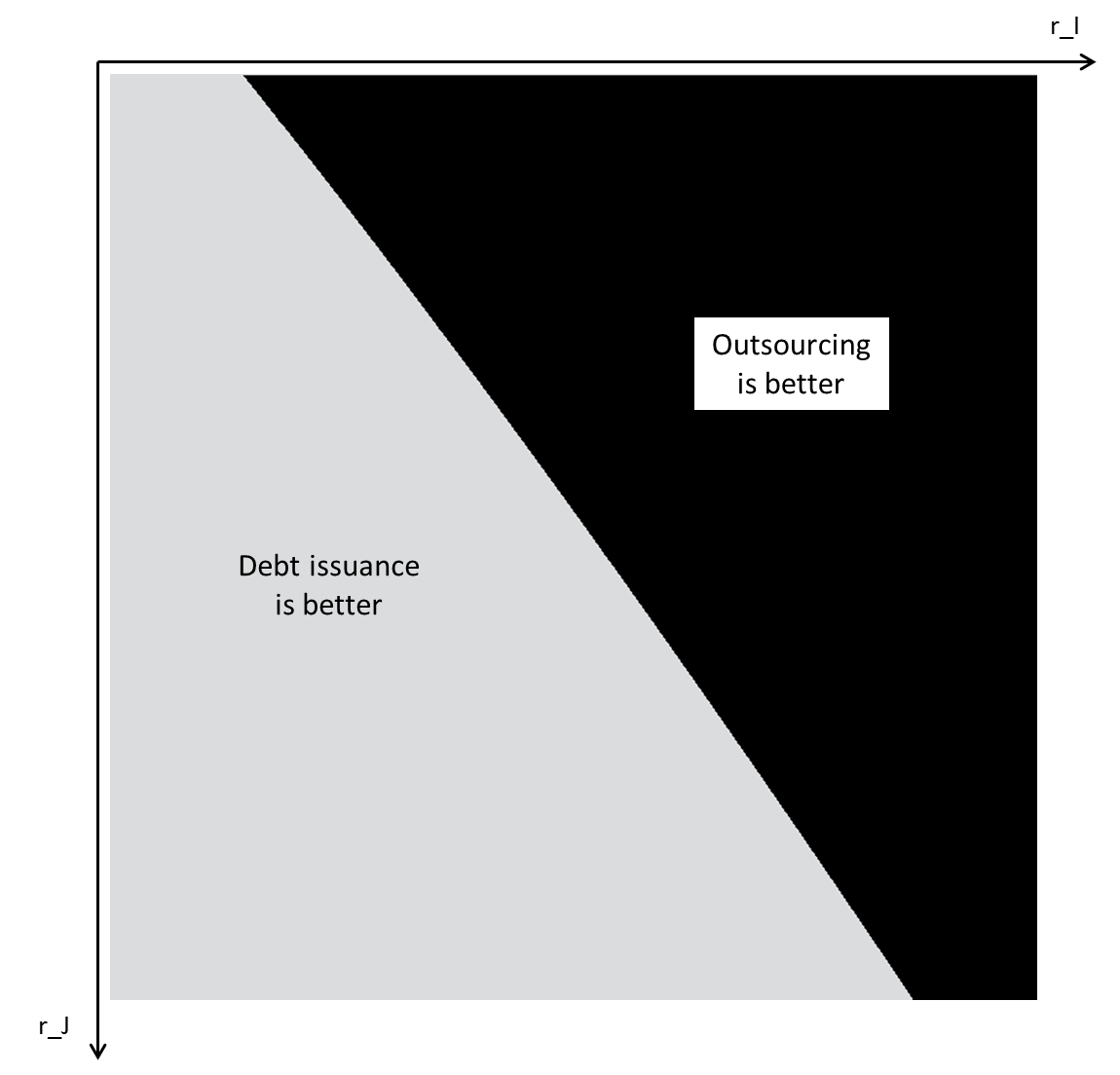
In comparison with Figure 3 dedicated to Nash equilibria, the boundary between the outsourcing and debt issuance regions has the same shape but the outsourcing region is slighly bigger.
4.3 Comparison Nash/Stackelberg equilibria
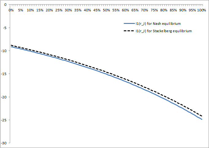
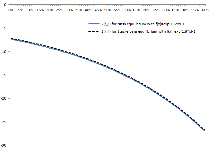
We first compare the value functions of firm between Nash and Stackelberg equilibria, in the situation of outsourcing the debt (Figure 6) and in the situation of debt issuance (Figure 7). In both situations, the value function is higher in Stackelberg equilibrium than in Nash equilibrium, which can be interpreted by the fact that firm has a leader position in Stackelberg equilibrium. The difference is a little less significant in Situation 2 than in Situation 1.
5 Proofs in Situation 1
5.1 Best responses in Situation 1
Let , and be given and constant. Then we get the following optimization problem for firm :
such that and using
| (35) |
Proposition 1
Let , and be given and constant. Then there exist optimal triplets for the above problem. Moreover is optimal if and only if it satisfies:
and
with and , where
| (36) |
Proof
We first need the following lemmas :
Lemma 2
The function is increasing, thus the equation admits the unique solution .