A study on analytic parametrizations for proton-proton cross-sections and asymptotia

Abstract

A comparative study on some representative parametrizations for the total and elastic cross-sections as a function of energy is presented. The dataset comprises $pp$ and $\bar{p}p$ scattering in the c.m energy interval 5 GeV - 8 TeV. The parametrization for the total cross-section at low and intermediate energies follows the usual reggeonic structure (non-degenerate trajectories). For the leading high-energy pomeron contribution, we consider three distinct analytic parametrizations: either a power ($P$) law, or a log-squared ($L2$) law or a log-raised-to-$\gamma$ ($L\gamma$) law, where the exponent $\gamma$ is treated as a real free fit parameter. The parametrizations are also extended to fit the elastic (integrated) cross-section data in the same energy interval. Our main conclusions are the following: (1) the data reductions with the logarithmic laws show strong dependence on the unknown energy scale involved, which is treated here either as a free parameter or fixed at the energy threshold; (2) the fit results with the $P$ law, the $L2$ law (free scale) and the $L\gamma$ law (fixed scale and exponent $\gamma$ above 2) are all consistent within their uncertainties and with the experimental data up to 7 TeV, but they partially underestimate the high-precision TOTEM measurement at 8 TeV; (3) once compared with these results, the $L2$ law with fixed scale is less consistent with the data and, in the case of a free scale, this pomeron contribution decreases as the energy increases below the scale factor (which lies above the energy cutoff); (4) in all cases investigated, the predictions for the asymptotic ratio between the elastic and total cross-sections, within the uncertainties, do not exceed the value 0.430 (therefore, below the black-disc limit) and the results favor rational limits between 1/3 and 2/5. We are led to conclude that the rise of the hadronic cross-sections at the highest energies still constitutes an open problem, demanding further and detailed investigation.

J. Phys. G: Nucl. Part. Phys. 40, 125001 (2013)

Table of Contents

1. Introduction

2. Formalism

2.1 Analytic Parametrizations for the Cross-Sections

2.1.1 Low-energy Contribution

2.1.2 High-energy Leading Contributions

2.2 Analytic Results for the $\rho$ Parameter

2.3 Summary and Notation

3. Fit Procedures and Results

3.1 Experimental Data and Fit Procedures

3.2 Results of the Individual Fits to Total Cross-Section and $\rho$ Data

3.3 Extensions to Elastic Cross-Section Data

3.3.1 Fit and Results

3.3.2 Asymptotic Ratios

4. Discussion

4.1 Preliminaries

4.2 Results for the Total Cross-Section and $\rho$

4.2.1 $L2$ Model versus $P$ Model

4.2.2 $L2$ Model versus $L\gamma$ Model

4.2.3 Conclusions on the Fit Results

4.3 Results for the Elastic Cross-Section and Asymptotia

4.3.1 Conclusions on the Fit Results

4.3.2 Asymptotia

5. Summary, Conclusions and Final Remarks

Appendix A. Derivative Dispersion Relations and the Subtraction Constant

A.1 Analytic Results

A.2 Comments on the Practical Use of Derivative Dispersion Relations

Appendix B. Global Fits to Total Cross-Section and $\rho$ Data

1 Introduction

The last 2 years represented a very fruitful period for the physics of the strong interactions at high energies. The advances are directly connected with the large amount of experimental data now available mainly from the Brookhaven-RHIC and the CERN-LHC (which has reached the 8 TeV maximal energy). However, despite the recent theoretical and experimental developments in several fronts of nuclear and particle physics, the soft strong interactions still constitute a great challenge for QCD [1, 2, 3].

In fact, in the absence of a pure (model-independent) QCD formalism able to predict the soft scattering states (elastic and diffractive processes), phenomenology is the approach expected to provide information for further theoretical developments in the large-distance sector. Nonetheless, it is an intrinsic characteristic of the phenomenological approach to present efficient descriptions of the experimental data through different physical assumptions, leading, in general, to distinct physical pictures [4, 5, 6, 7]. Whereas model predictions can be selected by some novel experimental data, phenomenological developments (additional or improved parameters) can adjust the model to the new experimental information. In a certain sense, this feedback process seems to permeate the phenomenological investigation of the elastic and diffractive scattering in the last decades. As a consequence, a widely accepted theoretical description of these soft hadronic processes still constitutes an open problem in the QCD context.

In the last years, the aforementioned situation has brought great expectations concerning the program developed by the TOTEM Collaboration at the CERN-LHC, since the aim of the experiment is just the investigation of the elastic and diffractive processes (single and double dissociation). Despite the intrinsic experimental and technical difficulties in reaching extremely small scattering angles, a large amount of data on several quantities has been made available recently. Of interest, here we quote the high-precision measurements of total and elastic (integrated) cross-sections at 7 and 8 TeV involving different methods and experimental conditions [8, 9, 10, 11].

In particle collisions, the total cross-section constitutes one of the most important physical quantities. As the sum of the elastic and inelastic cross sections, it provides fundamental information on the overall interaction process. In terms of the c.m. energy, the experimental data on the hadronic total cross-section ($\sigma_{\mathrm{tot}}$) are characterized by narrow peaks (resonances) in the region below $\sim$ 2 GeV, followed by a slow monotonic decrease as the energy increases in the scattering state region up to $\sim$ 20 GeV. From this region on, $\sigma_{\mathrm{tot}}$ grows smoothly and monotonically up to the highest energies with available data (see e.g. the plots in the Review of Particle Physics (RPP) by the Particle Data Group (PDG) [12], section 46).

Although the rise of $\sigma_{\mathrm{tot}}$ at high energies is an experimental fact, the theoretical (QCD) explanation for this increase and, most importantly, the exact energy dependence involved has been a long-standing problem. To some extent, the theoretical difficulty can be explained by the optical theorem since, through unitarity, it connects $\sigma_{\mathrm{tot}}$ with the imaginary part of the forward elastic scattering amplitude $F$ [2]:

$$\sigma_{\mathrm{tot}}(s)=\frac{\mathrm{Im}\,F(s,t=0)}{s},$$ (1)

where $s$ and $t$ are the Mandelstam variables. Therefore, formally, to obtain a theoretical result for $\sigma_{\mathrm{tot}}$ demands an input for $F(s,t)$, at least at $t=0$, and that presents a challenge for QCD, namely a soft scattering state and here in its simplest kinematic form the elastic channel.

In the absence of quantum field theory results for $\sigma_{\mathrm{tot}}(s)$, exclusively in terms of quarks and gluons, the theoretical investigation has been historically based on some general principles and formal results obtained in different contexts. These include Mandelstam representation, analyticity-unitarity-crossing concepts and axiomatic field theory leading, in general, to results expressed in terms of high-energy theorems and inequalities [13, 14, 15, 16, 17]. Among them, the Froissart-Martin bound for the total cross-section certainly plays a central role [18, 19, 20, 21, 22]:

$$\sigma_{\mathrm{tot}}(s)\leq c\ln^{2}\frac{s}{s_{h}},\qquad\mathrm{as}\qquad s\rightarrow\infty,$$ (2)

where $c\leq\pi/m_{\pi}^{2}\approx 60\,$ mb [23] and $s_{h}$ is an unknown constant. Although associated with numerical values far beyond the energies presently accessible in experiments, the result imposes a maximum rate of growth for the total cross-section with $s$, namely the log-squared bound at the asymptotic energy region. After the Martin derivation in the context of the axiomatic quantum field theory [21], this log-squared bound, associated with unitarity, has played a determinant role in model constructions, aimed to treat, interpret and describe soft strong interactions.

On the other hand, recently (2011), Azimov has demonstrated in a formal context that, depending on the assumed behavior for the scattering amplitude in the non-physical region, $\sigma_{\mathrm{tot}}$ may rise faster than log squared of $s$ without violation of unitarity [24, 25, 26]. Moreover, he has also argued that it is not obvious whether QCD can be considered an axiomatic field theory, since the latter demands asymptotic elementary free states and that contrasts with QCD confinement [24].

In the phenomenological context, an operational way to investigate the energy dependence of $\sigma_{\mathrm{tot}}$ has been the use of different analytic parametrizations, dictated or inspired by the analytic $S$-Matrix formalism and the Regge-Gribov theory [2, 3, 27, 28, 29, 30]. As we shall discuss in some detail, representative analytic forms include powers of $s$ and logarithmic dependencies on $s$ (linear and quadratic forms).

In this respect, the COMPETE Collaboration completed in 2002 a broad and detailed comparative investigation on different parametrizations, which turned out to be one of the most comprehensive amplitude analysis for hadron scattering [31, 32]. The approach comprised several classes of analytic parametrizations for the amplitude, different model assumptions and used all the forward data available at that time, on $pp$, $\bar{p}p$, mesons-$p$, $\gamma p$ and $\gamma\gamma$ scattering. A detailed quantitative procedure of ranking these models by the quality of the fit has been employed, including seven distinct statistical indicators as well as tests on different cutoff energies and on the universality of the leading high-energy contribution. With this ranking scheme, the log-squared parametrization, accounting for the rise of $\sigma_{\mathrm{tot}}$ at high energies, has been selected as the highest ranking model [31] (a conclusion corroborated by subsequent works [33, 34]). After that the selected COMPETE parametrization became a standard reference in successive editions of the RPP by the PDG [12, 35]. Moreover, a remarkable result concerns the fact that 10 years later [31], the COMPETE extrapolation for the $pp$ total cross-section at 7 TeV showed to be in complete agreement with the first high-precision measurement by the TOTEM Collaboration [8].

On the other hand, a rather intriguing result has been obtained by the PDG in the 2012 edition. The updated fit, with the log-squared COMPETE parametrization and including in the dataset the first 7 TeV TOTEM measurement of $\sigma_{\mathrm{tot}}$ [8], as well as the cosmic-ray data by the ARGO-YBJ Collaboration (at $\sim$ 100 - 400 GeV) [36] led to a data reduction not in complete agreement with the TOTEM datum. Indeed, from figure 46.10 in [12], the fit result, within the uncertainty, lies below the high-precision TOTEM measurement, despite the overall reduced chi-square of 0.96.

In the period 2011 - 2012, we developed several amplitude analyses, addressing the possibility of a different scenario for the rise of $\sigma_{\mathrm{tot}}$ at the highest energies [37, 38, 39]. This study was motivated by the above mentioned theoretical arguments by Azimov and was based on an analytical parametrization introduced by Amaldi et al in 1977, in which the exponent $\gamma$ of the leading logarithm contribution is not fixed at 2, but treated as a free real parameter of the fit [40]. This parametrization was also used by the UA4/2 Collaboration in 1993 [41] and in this respect, Matthiae stated [7]

“The principal aim is to derive from the data the value of the parameter $\gamma$ which controls the high-energy behaviour of the cross section and to make predictions at energies above those of the present accelerators.”

The analysis by Amaldi et al. with $pp$ and $\bar{p}p$ data up to $\sqrt{s}_{max}$ = 62 GeV indicated

$$\gamma=2.10\pm 0.10$$

and the subsequent analysis by the UA4/2 Collaboration, with data up to $\sqrt{s}_{max}$ = 546 GeV, yielded [41]

$$\gamma=2.25_{-0.31}^{+0.35}.$$

Although not statistically conclusive, these numerical values obtained for $\gamma$, within the corresponding uncertainties, seem to suggest the possibility of a rise of $\sigma_{\mathrm{tot}}$ faster than $\ln^{2}s$. Hence, on the basis of the theoretical arguments by Azimov and these empirical results, we understood that to address an investigation with the Amaldi parametrization and updated datasets (including the TOTEM data) could be a valid strategy. Our main point, as explicitly stated in [37], has been to attempt to look for answering two questions. Is the $\ln^{2}s$ dependence a unique solution describing the asymptotic rise of the total cross section? Could the data be statistically described by another solution, rising faster (or slower) than $\ln^{2}s$?

However, in this respect, there is a key issue: once $\gamma$ is treated as a real free parameter beyond the usual difficulties associated with the nonlinearity of the fit, we are also faced with the strong correlation among all the free parameters involved, especially an anti-correlation between $\gamma$ and a high-energy scaling parameter corresponding to the unknown constant $s_{h}$ in equation (2) (both, therefore, associated with the leading high-energy contribution). As a consequence, even obtaining solutions that are statistically consistent, we do not have uniqueness, namely we cannot provide a unique solution but only possible statistically consistent solutions (as discussed in some detail in [39], section 4.2).

Despite this limitation, under a variety of different conditions, fit procedures and datasets, we have obtained in [37], [38] and [39] several statistically consistent solutions, indicating a rise of $\sigma_{\mathrm{tot}}$ faster than the log-squared behavior at the LHC energy region (including all the recent TOTEM results at 7 and 8 TeV [39]). Moreover, and perhaps most importantly, extension of the parametrization for $\sigma_{\mathrm{tot}}$ to fit the elastic (integrated) cross section data, $\sigma_{\mathrm{el}}(s)$, led to asymptotic ratios between $\sigma_{\mathrm{el}}(s)$ and $\sigma_{\mathrm{tot}}$ below the black-disk limit (1/2) and consistent with the fractional limit 1/3 [38, 39]. Although answering, at least partially, the above mentioned two questions, the lack of unique solutions gives rise to some unavoidable critical discussions involving different points of view, as for example, those in [42] and in [43]. We shall return to the above two questions in our conclusions.

In this work, as one more step in our investigation, we present and discuss the results of a comparative study on some representative analytic parametrizations for $\sigma_{\mathrm{tot}}$. The focus here lies on (1) the consequences in the fit results imposed by the recent high-precision TOTEM measurements at 7 TeV and 8 TeV; (2) the extension of all the parametrizations to fit the elastic $\sigma_{\mathrm{el}}$ data (with the extraction of the asymptotic values for the ratio $\sigma_{\mathrm{el}}/\sigma_{\mathrm{tot}}$) and (3) discussions of the physical and phenomenological aspects involved.

As commented below, the analysis in the energy interval from 5 GeV up to 8 TeV is limited to $pp$ and $\bar{p}p$ data on $\sigma_{\mathrm{tot}}$, $\sigma_{\mathrm{el}}$ and the $\rho$ parameter defined by

$$\rho(s)=\frac{\mathrm{Re}\,F(s,t=0)}{\mathrm{Im}\,F(s,t=0)}.$$ (3)

The parametrization for $\sigma_{\mathrm{tot}}$ at low energies (below $\sim$ 20 GeV) consists of the usual Reggeon contributions associated with non-degenerate mesonic trajectories (power law of the energy with negative exponents). For the dominant term at high energies, responsible for the rise of $\sigma_{\mathrm{tot}}$ (pomeron contribution), we consider three independent forms: either a power law of $s$ with positive real exponent, or a log-squared of $s$ or a log-raised-to-$\gamma$ of $s$ with $\gamma$ a positive real exponent.

For the reasons to be discussed (and recalled) along the paper, our focus here is on individual fits to $\sigma_{\mathrm{tot}}$ data and the corresponding checks on the $\rho(s)$ behavior, using singly subtracted derivative dispersion relations (DDR). However, global fits to $\sigma_{\mathrm{tot}}$ and $\rho$ data are also presented and discussed in an appendix. Some results and detailed discussions present in our previous works [37, 38, 39] will be referred to and summarized along the paper.

Our main conclusions are as follows. Including in the dataset all the TOTEM measurements at 7 and 8 TeV, the results of the fits to $\sigma_{\mathrm{tot}}$ and $\rho$ data with the power and logarithmic laws ($\gamma$ = 2 or $\gamma$ above 2) are all almost statistically consistent within their uncertainties and with the experimental data up to 7 TeV. All the results, however, partially underestimate the high-precision TOTEM measurement at 8 TeV. In the case of the logarithmic forms, the high-energy-scale factor has a determinant role in the physical interpretations of the data reductions. In particular, the log-squared law with free scale leads to a decreasing pomeron contribution as the energy increases in the physical region between the cutoff ($\sqrt{s}_{min}$ = 5 GeV²) and the scale factor ($\sqrt{s}_{h}\approx$ 7 GeV²). That, however, is not the case with the other laws. In all cases investigated, the predictions for the asymptotic ratio between the elastic and total cross sections do not exceed the value 0.430 within the uncertainties, therefore, an upper bound below the black-disk limit.

The paper is organized as follows. In section 2, we treat the formal aspects of the analysis, displaying the analytic parametrizations for $\sigma_{\mathrm{tot}}(s)$ and $\rho(s)$ and discussing some phenomenological aspects involved. In section 3, the procedures and results of the fits are presented including the extensions to the elastic cross-section data. A detailed and critical comparative discussion of all results obtained here is the subject of section 4. Our conclusions and some final remarks are the contents of section 5. In appendix A, the analytical connection between $\sigma_{\mathrm{tot}}(s)$ and $\rho(s)$ is presented, together with some comments on the practical use of DDR and the role of the subtraction constant. Global (simultaneous) fits to $\sigma_{\mathrm{tot}}$ and $\rho$ data are addressed in appendix B.

2 Formalism

In this section, we introduce the analytic parametrizations to be used in our data reductions. Although well known by experts, we shall recall some basic physical concepts and interpretations [2, 3, 27, 28, 29, 30, 31, 32] that will help us to discuss and discriminate the result of the fits later in section 4.

2.1 Analytic parametrizations for the total cross-section

In the Regge-Gribov theory, for $s\rightarrow\infty$, the structure of the scattering amplitude in the $s$-channel is determined by its singularities in the complex $J$-plane ($t$-channel) [2, 3]. Simple poles give rise to a power-law behavior in $s$ and higher order poles results in logarithmic dependencies [3, 44]: $s\ln s$ (double pole), $s\ln^{2}s$ (triple pole), etc. Through the optical theorem (1), these structures constitute the basic choices in the analytic parametrizations of the hadronic total cross-section. In this context, the behavior of the $\sigma_{\mathrm{tot}}$ data above 5 GeV is usually represented by two components, associated with low-energy ($LE$) and high-energy ($HE$) contributions:

$$\sigma_{\mathrm{tot}}(s)=\sigma_{LE}(s)+\sigma_{HE}(s).$$ (4)

We shall discuss each case separately.

2.1.1 Low-energy contribution.

This term accounts for the decreasing of $\sigma_{\mathrm{tot}}$ in the region 5 GeV $\leq\sqrt{s}\lesssim$ 20 GeV and also for the differences between $pp$ and $\bar{p}p$ scattering. In the Regge-Gribov theory, this contribution is associated with Reggeon exchanges, namely the highest interpolated mesonic trajectories provided by spectroscopic data ($t$-channel), relating Re $J$ with the masses $M^{2}$ (the Chew-Frautschi plot). The trajectories are approximately linear defining an effective slope and intercept. The functional form for the total cross-section associated with a simple pole consists of a power law of $s$ with exponent (related with the intercept) around - 0.5. In its simplest and original version (Donnachie-Landshoff model [45, 46, 47]), this trajectory is degenerate, representing both $C=+1$ and $C=-1$ mesonic trajectories, namely ($a$, $f$) and ($\rho$, $\omega$), respectively. However, several amplitude analyses, including also both spectroscopic and scattering data, have indicated that the best data reductions are obtained with non-degenerate trajectories [48, 49, 50, 51, 52]. In this case and with our previous notation [37], the low-energy contribution can be expressed as

$$\sigma_{LE}(s)=a_{1}\,\left[\frac{s}{s_{l}}\right]^{-b_{1}}+\tau\,a_{2}\,\left[\frac{s}{s_{l}}\right]^{-b_{2}},$$ (5)

where $\tau$ = -1 (+1) for $pp$ ($\bar{p}p$) scattering, $s_{l}$ = 1 GeV² is fixed, while $a_{1}$, $b_{1}$, $a_{2}$ and $b_{2}$ are free fit parameters. In the phenomenological context, the parameters $a_{1}$ and $a_{2}$ are the reggeon residues (strengths) and $b_{1}$ and $b_{2}$ are associated with the intercepts of the trajectories (corresponding to simple poles at $J=1-b_{1}$ and $J=1-b_{2}$).

2.1.2 High-energy leading contributions.

The second term accounts for the rising of the total cross-section at higher energies and for our purposes, some comments on the different parametrizations to be considered here are appropriate.

Up to the beginning of the 1970s, the Reggeon contributions demonstrated good agreement with the smooth decrease of $\sigma_{\mathrm{tot}}$ data with the energy, demanding only an additional constant term to represent the asymptotic (Pomeranchuck) limit. However, new experimental results by the IHEP-CERN Collaboration at Serpukhov and subsequently at the CERN-ISR indicated the rise of $\sigma_{\mathrm{tot}}$ above $\sim$ 20 GeV. In the absence of a mesonic trajectory able to account for this rise, an ad hoc trajectory has been introduced, with intercept slightly greater than 1, namely an increasing contribution with the energy. This $C=+1$ trajectory (to account for an asymptotic equality between $pp$ and $\bar{p}p$ scattering) has been associated with a simple pole in the amplitude, corresponding, therefore, to a power law in $s$. Here, this parametrization for the total cross-section will be expressed and denoted as

$$\sigma_{HE}^{sp}(s)=\delta\,\left[\frac{s}{s_{h}}\right]^{\epsilon},$$ (6)

where $s_{h}$ = 1 GeV² is fixed, $\delta$ and $\epsilon$ are free parameters to be fitted and the superscript $sp$ stands for simple pole (at $J=1+\epsilon$).

Another possibility to explain the rise of $\sigma_{\mathrm{tot}}$ concerned the $\ln^{2}{s}$ behaviour, a result already suggested in the phenomenological context even before the experimental evidence of the rising total cross-section [53, 54]. Based on these and other indications [55, 56, 57] (perhaps also influenced by the log-squared bound by Froissart-Martin [3]), the higher order poles have come to take part in amplitude analyses [58, 59, 60, 61]. Here, as selected by the COMPETE Collaboration, we shall consider only the triple pole at $J=1$, parametrized and denoted by

$$\sigma_{HE}^{tp}(s)=\alpha+\beta\ln^{2}(s/s_{h}),$$ (7)

where $\alpha$, $\beta$ and the high-energy scale $s_{h}$ are free parameters of fit and the superscript $tp$ stands for triple pole.

At last, as commented in our introduction, we shall also consider an instrumental parametrization to address the possibility that the exponent in the logarithm contribution might not be exactly 2. To this end, we consider the power behaviour in $\ln{s}$ with a real exponent. This term, possibly associated with some kind of effective singularity in the amplitude, will be expressed by

$$\sigma_{HE}^{ef}(s)=\alpha+\beta\ln^{\gamma}(s/s_{h}),$$ (8)

where $\alpha$, $\beta$, $\gamma$ and $s_{h}$ are free fit parameters and the superscript $ef$ stands for effective.

At this point, it is already important to stress that parametrizations (6), (7) and (8) have different mathematical structures, different regions of validity, leading to distinct physical interpretations. A crucial point, not usually treated in the literature, concerns the presence of the high-energy-scale parameter $s_{h}$, as discussed in what follows (and also in section 4).

The $\sigma_{HE}^{sp}(s)$ parametrization already includes the physical condition $\epsilon>$ 0 to account for the rise of $\sigma_{\mathrm{tot}}$ (the original or standard soft pomeron concept). As a consequence, this term increases as the energy increases for all values of $s$, in particular in the region above the physical threshold for scattering states, namely $s\geq 4m_{p}^{2}$, where $m_{p}$ is the proton mass. Moreover, as a power law, the high-energy-scale factor $s_{h}$ can be absorbed by the $\delta$ parameter in data reductions, or be fixed at 1 GeV² (for dimensional reasons) as assumed here. Therefore, this parametrization does not depend on any energy-scale factor.

That, however, is not the case with the $\sigma_{HE}^{tp}(s)$ parametrization, since it increases with the energy only at $s>s_{h}$ (it is zero at $s=s_{h}$ and decreases as $s$ increases below $s_{h}$). Therefore, in this case, the strict physical interpretation of the pomeron exchange as responsible for the rise of the cross-section depends on the value of $s_{h}$ (fixed or fitted) and therefore, also on the value of the energy cutoff $\sqrt{s}_{min}$ for the data reductions.

At last, in what concerns the $\sigma_{\mathrm{HE}}^{ef}(s)$ parametrization, it is not defined as a real-valued function for $s<s_{h}$ and as a consequence cannot represent a physical quantity (total cross section). Therefore, in the physical context, equation (8) ought to be interpreted as a contribution just starting at $s=s_{h}$ with $\sigma_{\mathrm{HE}}^{ef}(s_{h})=\alpha$; from this point on, it increases as the energy increases (as in the standard soft pomeron concept).

We shall return to these different features of the high-energy parametrizations in our discussion of the fit results (section 4).

2.2 Analytic results for the $\rho$ parameter

With the parametrizations for $\sigma_{\mathrm{tot}}(s)$, the corresponding analytic results for $\rho(s)$ can be obtained by means of singly subtracted derivative dispersion relations (DDR). The subject is treated in some detail in appendix A, where discussions on the practical use of the derivative relations and the role of the subtraction constant involved are also presented. Here, we express the analytic results in a similar notation as that used for the total cross-section, including a term with the subtraction constant $K$ and two other additive terms ($T_{LE}(s)$ and $T_{HE}(s)$):

$$\rho(s) = \frac{1}{\sigma_{\mathrm{tot}}(s)}\left\{\frac{K}{s}+T_{LE}(s)+T_{HE}(s)\right\}.$$ (9)

The $T_{LE}(s)$ term is associated with the low-energy contribution and from appendix A, reads

$$T_{LE}(s)=-a_{1}\,\tan\left(\frac{\pi\,b_{1}}{2}\right)\left[\frac{s}{s_{l}}\right]^{-b_{1}}+\tau\,a_{2}\,\cot\left(\frac{\pi\,b_{2}}{2}\right)\left[\frac{s}{s_{l}}\right]^{-b_{2}},$$ (10)

where, as before, $\tau$ = -1 (+1) for $pp$ ($\bar{p}p$) scattering. For the $T_{HE}(s)$ term, we have the three forms (expressed with the corresponding superscripts $sp$, $tr$ and $ef$):

$$T_{HE}^{sp}(s)=\delta\,\tan\left(\frac{\pi\,\epsilon}{2}\right)\left[\frac{s}{s_{h}}\right]^{\epsilon},$$ (11)

$$T_{HE}^{tp}(s)=\pi\beta\ln\left(\frac{s}{s_{h}}\right),$$ (12)

$$T_{HE}^{ef}(s)=\mathcal{A}\,\ln^{\gamma-1}\left(\frac{s}{s_{h}}\right)+\mathcal{B}\,\ln^{\gamma-3}\left(\frac{s}{s_{h}}\right)+\mathcal{C}\,\ln^{\gamma-5}\left(\frac{s}{s_{h}}\right),$$ (13)

where

$$\mathcal{A}=\frac{\pi}{2}\,\beta\,\gamma,\quad\mathcal{B}=\frac{1}{3}\left[\frac{\pi}{2}\right]^{3}\,\beta\,\gamma\,[\gamma-1][\gamma-2],$$

$$\mathcal{C}=\frac{2}{15}\left[\frac{\pi}{2}\right]^{5}\,\beta\,\gamma\,[\gamma-1][\gamma-2][\gamma-3][\gamma-4].$$ (14)

In the last case, the third-order expansion is sufficient to ensure the convergence of the fit since, in practice (data reductions), the $\gamma$ values within the uncertainties lie below 2.5, as we shall show in section 3.

2.3 Summary and notation

In what follows, as a matter of notation and for short, we shall refer to the three cases of analytic parametrizations for $\sigma_{\mathrm{tot}}(s)$ by the corresponding laws associated with the high-energy contribution, namely

$P$ model, defined by equations (4), (5) and equation (6);

$L2$ model, defined by equations (4), (5) and equation (7);

$L\gamma$ model, defined by equations (4), (5) and equation (8).

In the first case, we have an extended Regge parametrization (the original Donnachie-Landshoff model but with non-degenerate trajectories), in the second case, the highest-rank parametrization selected by the COMPETE Collaboration and in the third case, the parametrization introduced by Amaldi et al.. Note that the COMPETE parametrization is a particular case of the Amaldi parametrization for $\gamma$ = 2 fixed. The corresponding analytic results for $\rho(s)$ are given by equations (9) - (14).

From our discussion on the high-energy leading contributions (section 2.1.2) and as defined above, models $P$ and $L2$ are analytically well defined for all values of $s$ and model $L\gamma$ only for $s\geq s_{h}$. (The region where $\ln^{\gamma}(s/s_{h})$ with $\gamma$ real, not integer, is a real valued function.) The practical effect of this analytical restriction in the data reductions will be discussed at the end of section 3.2.

3 Fit procedures and results

3.1 Experimental data and fit procedures

Several aspects of our methodology and fit procedures have been already presented and discussed in our previous analyses [37, 38, 39]. In what follows, we summarize the main points referring also to some other aspects of specific interest here.

1. The analysis is based only on the $pp$ and $\bar{p}p$ elastic scattering data in the energy interval from 5 GeV up to 8 TeV. The energy cutoff, $\sqrt{s}_{min}$ = 5 GeV, is the same used in the COMPETE and PDG analyses [12, 31, 32, 35]. The restriction to $pp$ and $\bar{p}p$ scattering means that we are dealing with only a subset of the reactions treated by the COMPETE and PDG analyses. However, it should be noted that $pp$ and $\bar{p}p$ scattering correspond to the cases of largest interval in energy with available data, giving therefore the most complete experimental information on particle-particle and antiparticle-particle collisions at the highest energies.

2. The input dataset for fits concerns only accelerator data on $\sigma_{\mathrm{tot}}$, $\rho$ and $\sigma_{\mathrm{el}}$. In addition to all the recent TOTEM measurements at 7 TeV (four $\sigma_{\mathrm{tot}}$ data and four $\sigma_{\mathrm{el}}$ data) and 8 TeV (one $\sigma_{\mathrm{tot}}$ datum and one $\sigma_{\mathrm{el}}$ datum) [8, 9, 10, 11], the experimental data below this energy region have been collected from the PDG database [62], without any kind of data selection or sieve procedure. Statistical and systematic errors have been added in quadrature. We note that the uncertainties in the TOTEM data are systematic (not statistical), resulting from the combination of the different contributions in quadrature and considering the correlations between them (table 7 in [9] and table IV in [11]). Estimations of the $pp$ total cross-section from cosmic-ray experiments will be displayed in the figures as illustrative results [36, 63, 64, 65]. The TOTEM estimation for $\rho$ at 7 TeV [10] is also displayed as illustration.

3. The data reductions have been performed with the objects of the class TMinuit of ROOT Framework [66]. We have employed the default MINUIT error analysis [67] with the selective criteria explained in [39] (section 2.2.4). In the data reductions, all the experimental points have been treated as independent, including the cases of more than one point at the same energy. The error matrix provides the variances and covariances associated with each free parameter, which are used in the analytic evaluation of the uncertainty regions associated with the fitted and predicted quantities (through standard error propagation procedures [68]). In our figures, these regions will be represented by a band, delimited by the upper and lower uncertainty extrema. As tests of goodness-of-fit, we shall consider the chi-square per degree of freedom ($\chi^{2}$/DOF) and the corresponding integrated probability, $P(\chi^{2})$ [68]. The goal is not to compare or select fit procedures or fit results but only to check the statistical consistence of each data reduction in a rather quantitative way.

4. As commented before, our main interest is not on global (or simultaneous) fits to $\sigma_{\mathrm{tot}}$ and $\rho$ data using dispersion relations. The main point, as in [37], concerns fits to $\sigma_{\mathrm{tot}}$ data and checks on the corresponding results for $\rho(s)$ using derivative dispersion relations, with the subtraction constant $K$ as a free fit parameter (see our discussion in appendix A.2). Specifically, after fitting the $\sigma_{\mathrm{tot}}$ data through equations (4) - (8), we fix the parameters to their central values in equations (9) - (14) for $\rho(s)$ and with only the subtraction constant $K$ as free parameter, we fit the $\rho$ data. We shall refer to this procedure as “individual fits to $\sigma_{\mathrm{tot}}$ and $\rho$ data”. Nonetheless, global fits are also treated as a complementary study in Appendix B and will be referred to in section 4.

5. The nonlinearity of the fits demands a choice of the initial values (feedbacks) for all free parameters [68]. Different choices have been tested and discussed in our previous analyses. In particular, among other choices, the results of the fits in the 2010 PDG version [35] have been used to initialize our parametric set in [37] and the results of the 2012 PDG version [12] in [38] and [39]. Here, given the excellent agreement between the 2002 COMPETE extrapolation and the recent TOTEM measurements at 7 and 8 TeV, we shall use the COMPETE numerical results [31] as initial values in our data reductions.

6. As discussed in detail in [39] (section 4.2), in the cases of the leading logarithm contributions ($\gamma$ = 2 or free), the energy scale factor $s_{h}$ plays a central role, not only in the data reductions but mainly in the physical interpretations of the results. For the reasons explained there, we also consider here two variants in the fit procedures: either $s_{h}$ as a free fit parameter or fixed to the energy threshold for the scattering states (above the resonance region), namely $s_{h}=4m_{p}^{2}$.

7. As in [38, 39], we also address the extension of the parametrizations for $\sigma_{\mathrm{tot}}$ to fit $\sigma_{\mathrm{el}}$ data. In this procedure, from the $s$-channel unitarity, the free exponents in the leading contributions at high energies, namely $\epsilon$ and $\gamma$, are fixed to their central fit values to $\sigma_{\mathrm{tot}}$ data.

In what follows, we treat the individual fits to $\sigma_{\mathrm{tot}}$ and $\rho$ data (section 3.2) and the extensions of the parametrizations to $\sigma_{\mathrm{el}}$ data (section 3.3). A critical discussion on all these results is presented in section 4.

3.2 Results of the individual fits to total cross-section and $\rho$ data

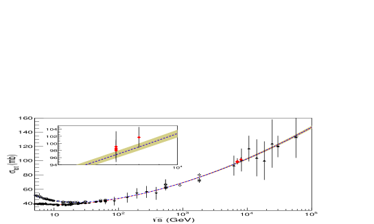
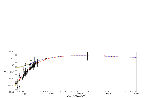
To initialize our parametric set to fit the $\sigma_{\mathrm{tot}}$ data, we use the 2002 COMPETE results, extracted from table VIII in [31] and associated with the models there denoted by RRE_nf (third column in that table) and RRP_nfL2_u (second column). The former set applies to our $P$ model and the latter to the $L2$ and $L\gamma$ models. The value of the parameters, in the case of $pp$ and $\bar{p}p$ scattering of interest here, are displayed in the second and fourth columns of our table 1. (The statistical information in the last lines of the table is explained in what follows.) The COMPETE results with these parameters and the corresponding parametrizations, are shown in figure 1, together with uncertainty regions evaluated through standard propagation from the errors in the parameters (table 1). In the figure, it is also displayed our accelerator dataset and the estimations from the cosmic-rays experiments (references in section 3.1, item 2). We shall discuss these COMPETE results together with our own fit results in section 4.

We note that in the case of model $L2$, the numerical values of the COMPETE parameters reported in [31] (our table 1) are not exactly the same as those reported in [32], which is the usual reference in the TOTEM Collaboration papers. The reason for our choice is the fact that in [31], the table provides the central values and uncertainties for both the $P$ and the $L2$ models, which is not the case in [32] (where only the central values for the $L2$ model are given). Moreover, since the main role of these parameters here is as initial values in data reductions, the small differences in the central values are not important.

Table 1: Fit results by the COMPETE Collaboration (2002 analysis) in the cases of our $P$ and $L2$ models for $pp$ and $\bar{p}p$ scattering, with the notation of equations (4) - (8) (extracted from table VIII in [31], models denoted RRE_nf and RRP_nfL2_u, respectively). The statistical information refers to the output of the first MINUIT run, corresponding to the central values of the parameters and the dataset used here (see text). The parameters $a_{1}$, $a_{2}$, $\alpha$, $\beta$ and $\delta$ are in mb, $s_{h}$ in GeV², $b_{1}$, $b_{2}$, $\gamma$ and $\epsilon$ are dimensionless ($s_{l}$ = 1 GeV²).

$P$ model $L2$ model (RREnf in [31]) (RRPnfL2u in [31]) $a_{1}$ 66.1 $\pm$ 1.2 $a_{1}$ 42.1 $\pm$ 1.3 $b_{1}$ 0.3646 $\pm$ 0.095 $b_{1}$ 0.467 $\pm$ 0.015 $a_{2}$ 35.3 $\pm$ 1.6 $a_{2}$ 32.19 $\pm$ 0.94 $b_{2}$ 0.5580 $\pm$ 0.0099 $b_{2}$ 0.5398 $\pm$ 0.0064 $\delta$ 18.45 $\pm$ 0.41 $\alpha$ 35.83 $\pm$ 0.40 $\epsilon$ 0.0959 $\pm$ 0.0021 $\beta$ 0.3152 $\pm$ 0.0095 $s_{h}$ 1 (fixed) $\gamma$ 2 (fixed) $s_{h}$ 34.0 $\pm$ 5.4 DOF 162 DOF 161 $\chi^{2}$/DOF 7.13 $\chi^{2}$/DOF 1.01 $P(\chi^{2})$ 2.57$\times$10-149 $P(\chi^{2})$ 0.442 Figure: 1 Figure: 1

Figure 1: Results for the $pp$ and $\bar{p}p$ total cross-sections from the 2002 COMPETE Collaboration analysis [31], with the parametrizations here denoted $P$ model (equations (4), (5) and (6)) and $L2$ model (equations (4), (5) and (7)). The values of the free parameters are displayed in table 1. The references to the accelerator data and cosmic-rays estimations are given in section 3.1 (item 2).

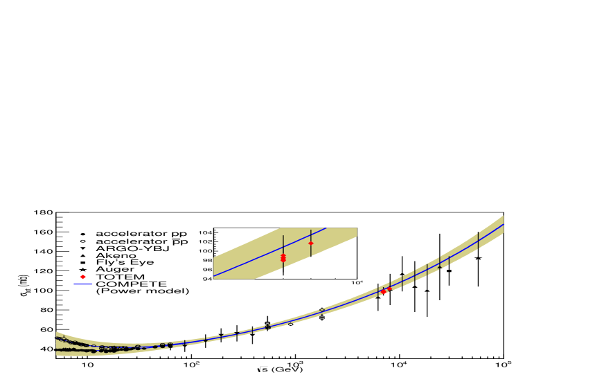
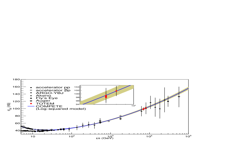
Differently from the COMPETE analysis, our ensemble consists of the $\sigma_{\mathrm{tot}}$ data from $pp$ and $\bar{p}p$ scattering in the energy interval 5 GeV - 8 TeV. For models $P$, $L2$ and $L\gamma$, we use as initial values the corresponding central values displayed in table 1. The first MINUIT run yields the $\chi^{2}$ for that ensemble and central values of the parameters; the final convergent run provides our fit result for that ensemble and model considered. The statistical information obtained in the first MINUIT run for the models $P$ and $L2$ (namely the COMPETE results with our ensemble) are displayed in the last lines of table 1.

For each model, after fitting the $\sigma_{\mathrm{tot}}$ data, we check the results for $\rho(s)$. In this case, we fix the resulting values of the parameters to their central values in equations (9) - (14) for $\rho(s)$ and then, with only the subtraction constant as a free parameter, we fit the $\rho$ data.

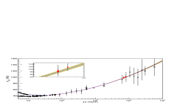
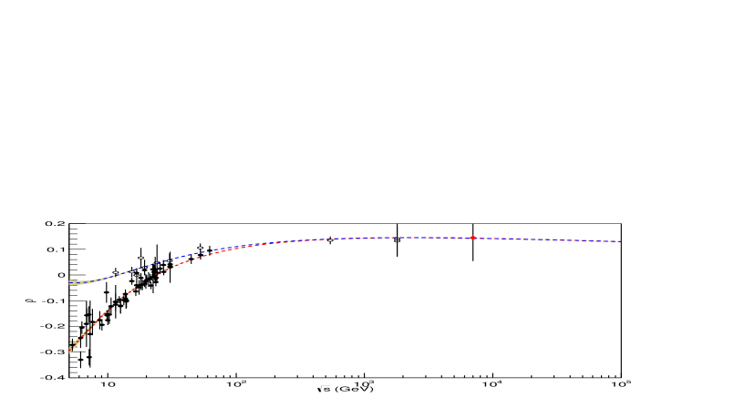
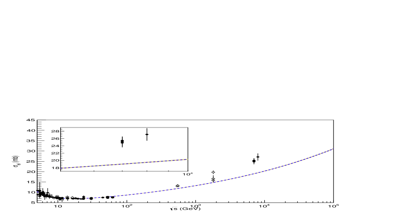
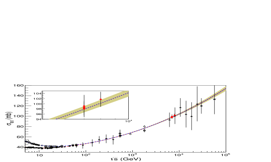
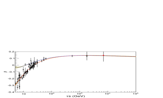
With this procedure our fit results with the $P$ model are displayed in table 2 (second and third columns) and in figure 2, together with the evaluated uncertainty regions and experimental information.

Table 2: Fit results with the $P$ model: individual fits to $\sigma_{\mathrm{tot}}$ and $\rho$ data and extentions to $\sigma_{\mathrm{el}}$ data. Units as in table 1.

$\sigma_{\mathrm{tot}}$ data $\rho$ data $\sigma_{\mathrm{el}}$ data $a_{1}$ 64.4 $\pm$ 1.8 64.4 72.4 $\pm$ 7.6 $b_{1}$ 0.364 $\pm$ 0.012 0.364 0.811 $\pm$ 0.028 $a_{2}$ 33.0 $\pm$ 2.3 33.0 0 (fixed) $b_{2}$ 0.539 $\pm$ 0.015 0.539 $-$ $\delta$ 18.94 $\pm$ 0.35 18.94 3.685 $\pm$ 0.021 $\epsilon$ 0.0926 $\pm$ 0.0016 0.0926 0.0926 (fixed) $K$ $-$ 24.0 $\pm$ 4.9 $-$ DOF 162 75 105 $\chi^{2}$/DOF 0.91 1.46 3.49 $P(\chi^{2})$ 0.794 5.91$\times$10-3 1.08$\times$10-30 Figure: 2 2 6

Figure 2: Results of the individual fits to $\sigma_{\mathrm{tot}}$ and $\rho$ data with the $P$ model (table 2). Legend on data as in figure 1.

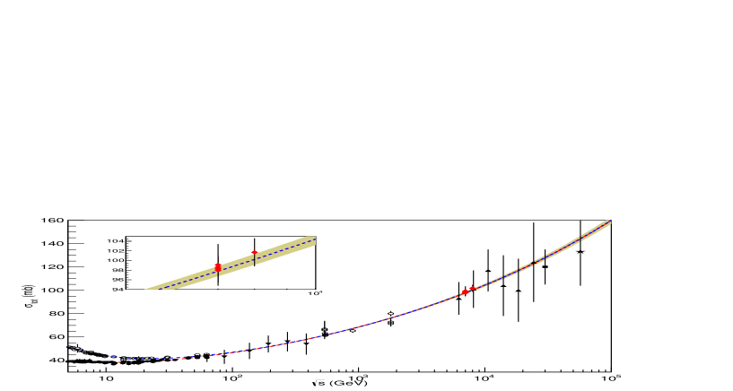
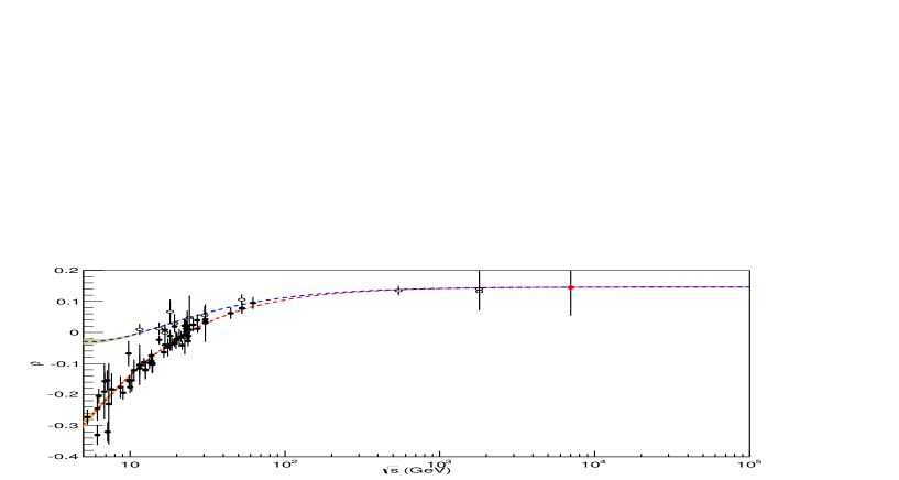
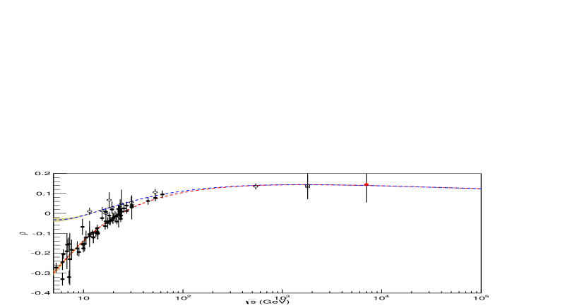
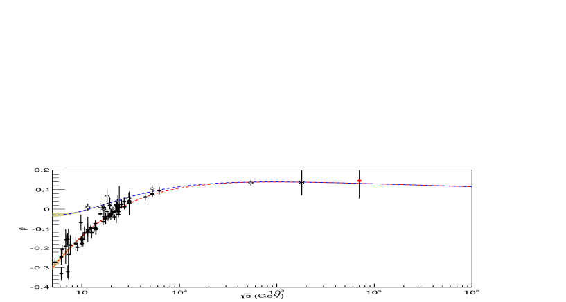
In the case of the $L2$ model, we consider two variants, either the high-energy-scale factor $s_{h}$ as a free parameter or fixed to the energy threshold $s_{h}=4m_{p}^{2}$. The results with the former variant are displayed in table 3 (second and third columns) and figure 3 and those with the latter variant are shown in table 4 (second and third columns) and figure 4.

Although the same two variants had been considered with the $L\gamma$ model, we did not obtain full convergence in the case of $s_{h}$ as a free fit parameter, but only for $s_{h}=4m_{p}^{2}$ fixed. We understand that this effect can be explained as follows.

As discussed in section 2.3, model $L\gamma$ is well defined only for $s\geq s_{h}$. In practice (data reductions through the MINUIT code), if this condition is not satisfied in the physical region above the cutoff, the fit does not converge (because $\ln^{\gamma}(s/s_{h})$ is not a real-valued function). Now, from table 3, in the case of the $L2$ model with $s_{h}$ free, we see that the fit value of this parameter is somewhat large, $s_{h}\sim$ 40 GeV², lying, therefore, in the physical region of the data reduction, above the cutoff $s_{min}$ = 25 GeV². Due to the strong anti-correlation between the fit parameters $\gamma$ and $s_{h}$, the data reduction favors larger values of $s_{h}$ which can reach the physical region (beyond the cutoff), where the $\ln^{\gamma}(s/s_{h})$ term is not defined, resulting, therefore, in no convergence. We understand that this trend of the data reductions is also connected with the rather large value of the high-precision TOTEM measurement at 8 TeV. In fact, as we have shown in [39], if this point is not included in the dataset (the $\sqrt{s}_{max}$ = 7 TeV Ensemble in [39]), full convergence is obtained and $s_{h}$ as free parameter lies below the cutoff $s_{min}$ = 25 GeV². However, once included in the dataset, no convergence is obtained.

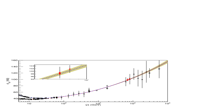
Therefore, with the dataset here considered, the $L\gamma$ model applies only for $s_{h}=4m_{p}^{2}$ fixed. Note, however, that since the region $s<s_{h}=4m_{p}^{2}$ (below the threshold) constitutes a non-physical region, in this case, model $L\gamma$ is well defined in the whole physical region of scattering states. The corresponding fit results are displayed in table 5 (second and third columns) and figure 5.

Table 3: Fit results with the $L2$ model and $s_{h}$ as a free parameter: individual fits to $\sigma_{\mathrm{tot}}$ and $\rho$ data and extentions to $\sigma_{\mathrm{el}}$ data. Units as in table 1.

$\sigma_{\mathrm{tot}}$ data $\rho$ data $\sigma_{\mathrm{el}}$ data $a_{1}$ 56.2 $\pm$ 7.3 56.2 117 $\pm$ 66 $b_{1}$ 0.588 $\pm$ 0.087 0.588 1.17 $\pm$ 0.19 $a_{2}$ 33.2 $\pm$ 2.3 33.2 0 (fixed) $b_{2}$ 0.541 $\pm$ 0.016 0.541 $-$ $\alpha$ 37.1 $\pm$ 1.3 37.1 6.82 $\pm$ 0.12 $\beta$ 0.312 $\pm$ 0.021 0.312 0.1200 $\pm$ 0.0064 $\gamma$ 2 (fixed) 2 2 (fixed) $s_{h}$ 43 $\pm$ 23 43 219 $\pm$ 60 $K$ $-$ 48.3 $\pm$ 4.9 $-$ DOF 161 75 103 $\chi^{2}$/DOF 0.91 1.47 1.55 $P(\chi^{2})$ 0.778 5.16$\times$10-3 2.91$\times$10-4 Figure: 3 3 7

Table 4: Fit results with the $L2$ model and $s_{h}=4m_{p}^{2}$ fixed: individual fits to $\sigma_{\mathrm{tot}}$ and $\rho$ data and extentions to $\sigma_{\mathrm{el}}$ data. Units as in table 1.

$\sigma_{\mathrm{tot}}$ data $\rho$ data $\sigma_{\mathrm{el}}$ data $a_{1}$ 52.1 $\pm$ 2.1 52.1 270.5 $\pm$ 2.9 $b_{1}$ 0.392 $\pm$ 0.019 0.392 0.480 $\pm$ 0.038 $a_{2}$ 33.0 $\pm$ 2.2 33.0 0 (fixed) $b_{2}$ 0.539 $\pm$ 0.015 0.539 $-$ $\alpha$ 29.75 $\pm$ 0.47 29.75 3.68 $\pm$ 0.23 $\beta$ 0.2476 $\pm$ 0.0049 0.2476 0.0756 $\pm$ 0.0023 $\gamma$ 2 (fixed) 2 2 (fixed) $s_{h}$ 3.521 (fixed) 3.521 3.521 (fixed) $K$ $-$ 21.9 $\pm$ 4.9 $-$ DOF 162 75 104 $\chi^{2}$/DOF 0.93 1.45 1.72 $P(\chi^{2})$ 0.718 6.71$\times$10-3 7.77$\times$10-6 Figure: 4 4 8

Figure 3: Results of the individual fits to $\sigma_{\mathrm{tot}}$ and $\rho$ data with the $L2$ model and $s_{h}$ free (table 3). Legend on data as in figure 1.

Figure 4: Results of the individual fits to $\sigma_{\mathrm{tot}}$ and $\rho$ data with the $L2$ model and $s_{h}=4m_{p}^{2}$ fixed (table 4). Legend on data as in figure 1.

Table 5: Fit results with the $L\gamma$ model and $s_{h}=4m_{p}^{2}$ fixed: individual fits to $\sigma_{\mathrm{tot}}$ and $\rho$ data and extentions to $\sigma_{\mathrm{el}}$ data. Units as in table 1.

$\sigma_{\mathrm{tot}}$ data $\rho$ data $\sigma_{\mathrm{el}}$ data $a_{1}$ 60.9 $\pm$ 7.8 60.9 348.3 $\pm$ 4.9 $b_{1}$ 0.530 $\pm$ 0.071 0.530 0.616 $\pm$ 0.043 $a_{2}$ 33.2 $\pm$ 2.3 33.2 0 (fixed) $b_{2}$ 0.541 $\pm$ 0.016 0.541 $-$ $\alpha$ 34.1 $\pm$ 1.4 34.1 4.93 $\pm$ 0.13 $\beta$ 0.102 $\pm$ 0.040 0.102 0.03122 $\pm$ 0.00081 $\gamma$ 2.30 $\pm$ 0.14 2.30 2.30 (fixed) $s_{h}$ 3.521 (fixed) 3.521 3.521 (fixed) $K$ $-$ 45.1 $\pm$ 4.9 $-$ DOF 161 75 104 $\chi^{2}$/DOF 0.91 1.48 1.62 $P(\chi^{2})$ 0.788 4.22$\times$10-3 7.16$\times$10-5 Figure: 5 5 9

Figure 5: Results of the individual fits to $\sigma_{\mathrm{tot}}$ and $\rho$ data with the $L\gamma$ model and $s_{h}=4m_{p}^{2}$ fixed (table 5). Legend on data as in figure 1.

3.3 Extensions to elastic cross-section data

The connection between the total cross-section and the forward elastic amplitude (optical theorem) led us in [38, 39] to explore the possibility to extend the same $L\gamma$ model (with $\gamma$ above 2) to fit the elastic cross-section data (see section 3 in [38] for more details). Here we address this extension taking into account the three models considered.

A noticeable difference between the $\sigma_{\mathrm{tot}}$ and $\sigma_{\mathrm{el}}$ data concerns the low-energy region, where the evident differences involving $pp$ and $\bar{p}p$ scattering in the former case are not observed in the latter. For that reason, to extend the parametrization we consider a degenerate trajectory in the $\sigma_{LE}(s)$ contribution, namely we fix $a_{2}$ = 0 in all models.

Concerning the $\sigma_{HE}(s)$ contribution, since the optical theorem is directly related to unitarity, in applying the same model for $\sigma_{\mathrm{tot}}$ to fit the $\sigma_{\mathrm{el}}$ data, this principle cannot be violated, namely for $s\rightarrow\infty$, the ratio $\sigma_{\mathrm{el}}$/$\sigma_{\mathrm{tot}}$ can not go to infinity; moreover, a scenario of an asymptotic transparent disk, namely $\sigma_{\mathrm{el}}$/$\sigma_{\mathrm{tot}}(s)\rightarrow 0$, is also not expected. As a consequence, in the case of the $P$ and $L\gamma$ models, the same values of the exponents in the leading high-energy contribution ($\epsilon$ and $\gamma$) obtained with the $\sigma_{\mathrm{tot}}$ fit must be considered for the $\sigma_{\mathrm{el}}$ data reduction.

It is also important to note that, although based on unitarity arguments, our extension of the parametrization from $\sigma_{\mathrm{tot}}(s)$ to $\sigma_{\mathrm{el}}(s)$ has here a strictly empirical character. In particular, Regge models have their own results for the elastic differential cross-section and consequently for the corresponding integrated elastic cross-sections. Therefore, in this section, the three models will be considered only as empirical parametrizations.

3.3.1 Fit and results

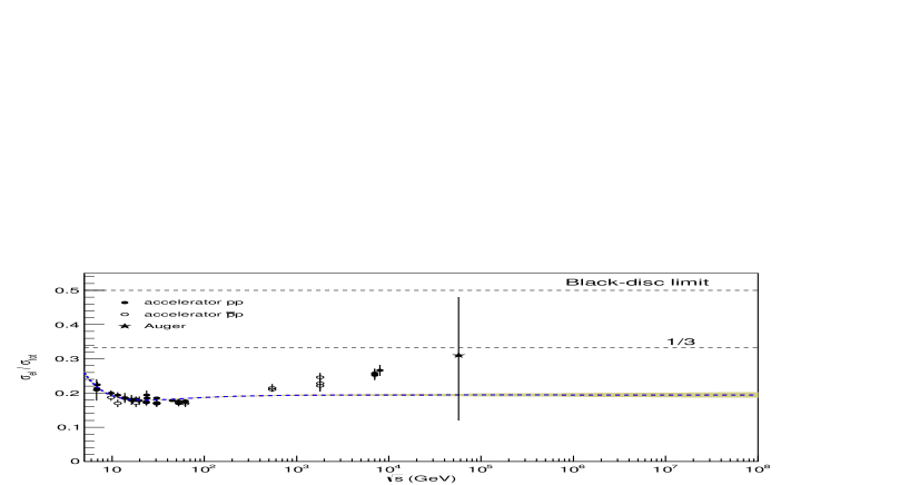
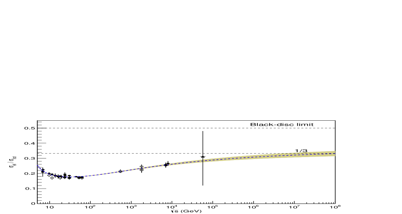
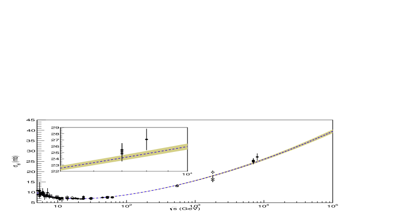
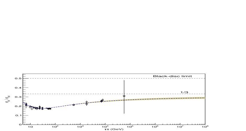
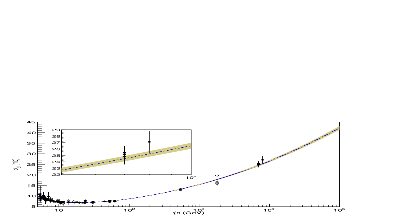
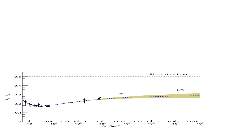
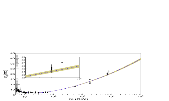
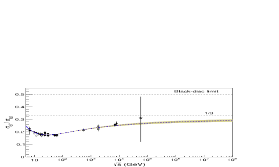
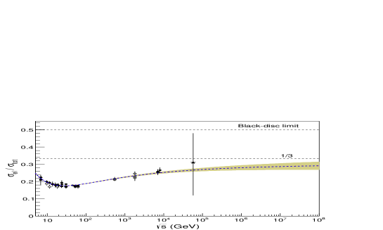
Based on the above discussion, in extending the $P$ model to $\sigma_{\mathrm{el}}$ we fix $\epsilon$ = 0.0926 (table 2) and in the case of the $L\gamma$ model, $\gamma$ = 2.30 is fixed (table 5). As initial values, including the $L2$ model with the two variants, we use the central values of the parameters obtained in the corresponding fits to $\sigma_{\mathrm{tot}}$ data (second columns in tables 2, 3, 4 and 5). With this procedure, we obtain the fit results displayed in the fourth columns of tables 2, 3, 4 and 5 and in the upper panels of figures 6, 7, 8, 9. In the lower panels of these figures we show the corresponding predictions for the ratios between the elastic and total cross-sections. Using the $s$-channel unitarity, we have also included in these plots the result from the estimations of the total cross-section and the inelastic cross-section ($\sigma_{\mathrm{inel}}$) at 57 TeV by the Auger Collaboration [65].

Figure 6: Result of the fit to the elastic cross-section data with the $P$ model and predictions for the ratio between the elastic and total cross-sections (table 2, fourth column).

Figure 7: Result of the fit to the elastic cross-section data with the $L2$ model in the case of $s_{h}$ free and predictions for the ratio between the elastic and total cross-sections (table 3, fourth column).

Figure 8: Result of the fit to the elastic cross-section data with the $L2$ model in the case of $s_{h}=4m_{p}^{2}$ fixed and predictions for the ratio between the elastic and total cross-sections (table 4, fourth column).

Figure 9: Result of the fit to the elastic cross-section data with the $L\gamma$ model in the case of $s_{h}=4m_{p}^{2}$ fixed and prediction for the ratio between the elastic and total cross-sections (table 5, fourth column).

3.3.2 Asymptotic ratios

With the analytic parametrizations (4) - (8), the value of asymptotic ratio between the elastic and total cross-sections can be evaluated. They are related to the parameters $\delta$ ($P$ model) and $\beta$ ($L2$ and $L\gamma$ models). Denoting these parameters by the corresponding subscripts associated with $\sigma_{\mathrm{el}}$ and $\sigma_{\mathrm{tot}}$ fits, for $s\rightarrow\infty$ we have

$$\frac{\sigma_{\mathrm{el}}}{\sigma_{\mathrm{tot}}}\rightarrow\frac{\delta_{\mathrm{el}}}{\delta_{\mathrm{tot}}}\quad[P\ \mathrm{model}],\quad\frac{\sigma_{\mathrm{el}}}{\sigma_{\mathrm{tot}}}\rightarrow\frac{\beta_{\mathrm{el}}}{\beta_{\mathrm{tot}}}\quad[L2\ \mathrm{and}\ L\gamma\ \mathrm{models}].$$ (15)

From tables 2 - 5 we obtain the values displayed in table 6.

Table 6: Asymptotic results for the ratio $\sigma_{\mathrm{el}}/\sigma_{\mathrm{tot}}$ obtained from the individual fits to $\sigma_{\mathrm{tot}}$ data and the extensions to $\sigma_{\mathrm{el}}$ data, equation (15).

Model Asymptotic Ratio $\sigma_{\mathrm{el}}/\sigma_{\mathrm{tot}}$ $P$ 0.1945 $\pm$ 0.0038 $L2$, $s_{h}$ free 0.385 $\pm$ 0.033 $L2$, $s_{h}$ fixed 0.305 $\pm$ 0.011 $L\gamma$, $s_{h}$ fixed 0.31 $\pm$ 0.12

4 Discussion

4.1 Preliminaries

Before discussing all results presented in section 3, it is important to keep in mind four fundamental differences between the COMPETE analysis and the one developed here.

First, our dataset, restricted to $pp$ and $\bar{p}p$ scattering, constitutes only a sub-set of the data analyzed by the COMPETE Collaboration. We did not take into account any constraint dictated by other reactions at low and intermediate energies or a supposed universal behavior.

Second, the COMPETE analysis on $\sigma_{\mathrm{tot}}$ covered the energy region up to $\sqrt{s}_{max}$ = 1.8 TeV. This maximal energy is characterized by the disagreement between the measurement by the CDF Collaboration [70] and the two measurements by the E710 and E811 Collaborations [71,72]. In fact, as stated in [72], “the confidence level that all 3 measurements are compatible is only 1.6 %”. On the other hand, our dataset includes all the high-precision TOTEM measurements at 7 TeV (4 points) and 8 TeV (1 point).

Third, the COMPETE has employed a detailed procedure of ranking models, including seven distinct statistical indicators. In our case, only the $\chi^{2}$/DOF and $P(\chi^{2})$ have been used to check the statistical consistency of the data reductions in a reasonable way.

Fourth, taking into account several classes of analytic parametrizations and constraints, the COMPETE Collaboration investigated 256 variants, selecting 24 possible models under the criteria of $\chi^{2}$/DOF $\leq$ 1.0 and non-negative pomeron contribution at all energies [31]. Among those models they have eventually selected their highest rank parametrization. Here, we have restricted our analysis to only three analytic models (and two variants in one case). Nonetheless, the novel aspect concerns the use of the parametrization introduced by Amaldi et al., which, unfortunately, did not take part in the COMPETE analysis.

Bearing in mind the above differences, let us now discuss all the results presented in section 3, including reference to some results by the COMPETE Collaboration. We shall discuss separately the data reductions for the total cross-section and $\rho$ parameter (section 4.2) and the elastic cross-section (section 4.3).

4.2 Results for the total cross-section and $\rho$

The main point here is to confront the results obtained through model $L2$ with those provided by models $P$ and $L\gamma$. To this end, we divide the discussion as follows.

4.2.1 $L2$ model versus $P$ model

Let us start with the COMPETE results displayed in figure 1, table 1, related to the $P$ model and the $L2$ model. Although both extrapolations led to good agreement with the TOTEM results, within the uncertainties, the compatibility in the case of the $L2$ model, especially at 8 TeV, is indeed striking. Even the statistical result with our dataset is quite good: $\chi^{2}$/DOF = 1.01 (table 1). We note, however, that in the COMPETE result, $s_{h}\sim$ 34 GeV² which means that with the assumed energy cutoff at $s_{min}$ = 25 GeV², the leading $L2$ pomeron contribution decreases as the energy increases in the region from $s_{min}$ up to $s_{h}$ (as already discussed in [39], section 4.2, figure 7).

With regard to the $P$ model predictions, if compared with the above $L2$ model result, the extrapolation, although in agreement with the TOTEM data within the uncertainties, overestimates the central values of the TOTEM results at 7 and 8 TeV (figure 1). We recall that in [32], the COMPETE Collaboration does not consider this model and in [31], the authors conclude that it “fails to reproduce jointly the total cross section and the $\rho$ parameter for $\sqrt{s}\geq$ 5 GeV”.

Let us turn now to our fit results with the dataset here considered: table 2 and figure 2 ($P$ model) and tables 3, 4, figures 3, 4 ($L2$ model in the cases of $s_{h}$ free and fixed, respectively). Here, the situation is rather different, since in both cases, the fit results are essentially equivalent on statistical grounds: $P(\chi^{2})\approx$ 0.8 with the $P$ model and $L2$ model in the case of $s_{h}$ free and $P(\chi^{2})\approx$ 0.7 with the $L2$ model and $s_{h}$ fixed. Moreover, in the LHC region, the results of the $P$ model and the $L2$ model ($s_{h}$ free) are practically identical (figures 2 and 3): the upper band of the fit uncertainty region includes the central values of the TOTEM data at 7 TeV and the upper extreme of the band reaches the central value of the datum at 8 TeV. The same equivalence can be verified in the corresponding results for $\rho(s)$ and the descriptions of the data are quite good. However, we note that, as in the COMPETE result, the $L2$ model with $s_{h}$ free yields $s_{h}\sim$ 43 GeV² (table 3) and therefore a decreasing pomeron contribution between $s_{min}$ = 25 GeV² and $s_{h}$. That obviously is not the case with the $P$ model, since it brings enclosed the rise of the leading high-energy contribution at all energies.

On the other hand, compared with the above results, the $L2$ model in the case of $s_{h}=4m_{p}^{2}\sim$ 3.5 GeV² fixed (far below the cutoff) partially underestimates the TOTEM data (including the central value of the $\rho$ estimation at 7 TeV), as shown in figure 4 and discussed below in section 4.2.2.

We note that, with the $P$ model, the value of the soft pomeron intercept obtained here reads $\alpha_{\mathcal{P}}(0)=1+\epsilon=1.0926\pm 0.0016$. This result can be compared with those reported in some previous analyses, as shown in table 7 ($\sqrt{s}_{max}$ = 1.8 TeV). We see that, within the uncertainties, our result is in agreement with those obtained by Cudell, Kang and Kim, also by Cudell et al. and with the extrema bounds inferred by Luna and Menon; our result lies slightly below the COMPETE result (table 1) and above the historical value by Donnachie and Landshoff (degenerate trajectories).

Table 7: Values of the soft pomeron intercept ($\alpha_{\mathcal{P}}(0)=1+\epsilon$) from some previous analyses and from this work.

$\alpha_{\mathcal{P}}(0)$ Donnachie-Landshoff (1992) [47] 1.0808 Cudell, Kang and Kim (1997) [49] 1.096${}_{-0.009}^{+0.012}$ Cudell et al. (2000) [61] 1.093 $\pm$ 0.003 COMPETE Collaboration (2002) [31] 1.0959 $\pm$ 0.0021 Luna and Menon (2003) [51] 1.085 - 1.104 This work 1.0926 $\pm$ 0.0016

4.2.2 $L2$ model versus $L\gamma$ model

With the $L\gamma$ model we obtain a convergent fit solution only in the case of $s_{h}$ fixed. Therefore, our comparative discussion with the $L2$ model will be restricted here to this variant (individual and global fits).

As regards individual fits, from tables 4 and 5, with the $L2$ model $P(\chi^{2})\approx$ 0.72 and in the case of the $L\gamma$ model, $P(\chi^{2})\approx$ 0.79, indicating, therefore, a practical equivalence on statistical grounds. On the other hand, noticeable differences can be identified in the LHC region, as shown in figures 4 and 5. In the case of the $L2$ model (figure 4), the fit uncertainty region shows agreement with only the lower error bar of the TOTEM results at 7 TeV and the upper extreme of the band does not reach the central value of the datum at 8 TeV. That, however, is not the case with the $L\gamma$ model (figure 5), since the uncertainty region includes all the central values of the data at 7 TeV and the upper band reaches the central value at 8 TeV.

With these models and variant, we have also developed simultaneous fits to $\sigma_{\mathrm{tot}}$ and $\rho$ data, which are presented in appendix B: table 8 (second and fourth columns) and figures 11 and 12. In both cases, we obtain a smaller integrated probability, $P(\chi^{2})\approx$ 0.2, which is a consequence of the inclusion of the $\rho$ data. From the figures, the results at the LHC region are practically identical to those obtained in the individual fits.

With the $L\gamma$ model, in going from individual to global fits, we notice a slightly decrease in the $\gamma$ parameter, from 2.30 (table 5) to 2.23 (table 8). This difference is also due to the inclusion of the $\rho$ data, which constraint the rise of the total cross section (see our discussion in A.2).

4.2.3 Conclusions on the fit results

Based on the results presented here and on the above discussion, we are led to the conclusions that follow.

1. The fit results with the $P$ model, the $L2$ model (in the case of $s_{h}$ free) and the $L\gamma$ model ($s_{h}$ fixed) are all consistent within their uncertainties, leading to equivalent descriptions of the experimental data. That means three different possible scenarios for the rise of the total cross-section at the highest energies.

2. In all cases above, the fit results are not in plenty agreement with the TOTEM datum at 8 TeV: within the uncertainties, the data reductions partially underestimate this high-precision measurement.

3. Compared with the results mentioned above, the $L2$ model with the variant $s_{h}$ fixed leads to fit results less consistent with the experimental data. In the case of $s_{h}$ free, however, the leading pomeron contribution decreases as the energy increases below $\sqrt{s_{h}}\approx$ 7 GeV (table 3).

4. As regards models $P$ and $L\gamma$, in addition to their efficiency in the description of the experimental data (except, perhaps, at 8 TeV), both bring enclosed an increasing pomeron contribution for all values of the energy (above the threshold $4m_{p}^{2}$ in the last case).

5. For $s_{h}=4m_{p}^{2}$ fixed, model $L\gamma$ is well defined in the whole physical region of scattering states and the fit results are more consistent with the $\sigma_{tot}$ data at 7 and 8 TeV than model $L2$ (figures 4 and 5 and also 11 and 12).

4.3 Results for the elastic cross-section and asymptotia

4.3.1 Conclusions on the fit results.

Concerning the $P$ model here considered, despite the efficient descriptions of the $\sigma_{\mathrm{tot}}$ and $\rho$ data, it is certainly not adequate to be extended to fit the $\sigma_{\mathrm{el}}$ data with $\epsilon$ fixed, as shown in table 2 (fourth column) and figure 6. We have displayed these results only as a complementary information and we shall not refer to them in what follows.

In the cases of the $L2$ and $L\gamma$ models, despite the rather small integrated probabilities (tables 3, 4 and 5, fourth columns), the description of the experimental data below the LHC region is quite good in all cases (figures 7, 8 and 9). The differences (and drawbacks) concern the TOTEM results at 7 TeV (four points) and 8 TeV (one point), as shortly discussed in what follows.

With the $L2$ model and $s_{h}$ free (fig. 7), the TOTEM data at 7 TeV are quite well described within the uncertainties and the fit uncertainty region includes part of the lower error bar at 8 TeV. The corresponding prediction for the ratio $\sigma_{\mathrm{el}}$/$\sigma_{\mathrm{tot}}$ is also in good agreement with the TOTEM data at 7 and 8 TeV, within the uncertainties.

In the case of $s_{h}$ fixed (fig. 8) the uncertainty region of the fit with the $L2$ model is consistent with the lower error bar at 7 TeV, but does not reach the lower error bar at 8 TeV. Analogous results are obtained with the $L\gamma$ model (fig. 9), except that, in this case, the fit uncertainty region reaches the lower error bar at 8 TeV.

We have also extended to $\sigma_{\mathrm{el}}$ the results obtained in global fits to $\sigma_{\mathrm{tot}}$ and $\rho$ data with the $L2$ and $L\gamma$ models ($s_{h}$ fixed), presented in Appendix B. From table 8 (third and fifth columns) and figures 11 and 12, we are led to the same conclusions outlined above.

Figure 10: Asymptotic ratios between the elastic and total cross-sections obtained in this analysis and combining the TOTEM and COMPETE results (tables 6, 9 and equation (16)).

4.3.2 Asymptotia.

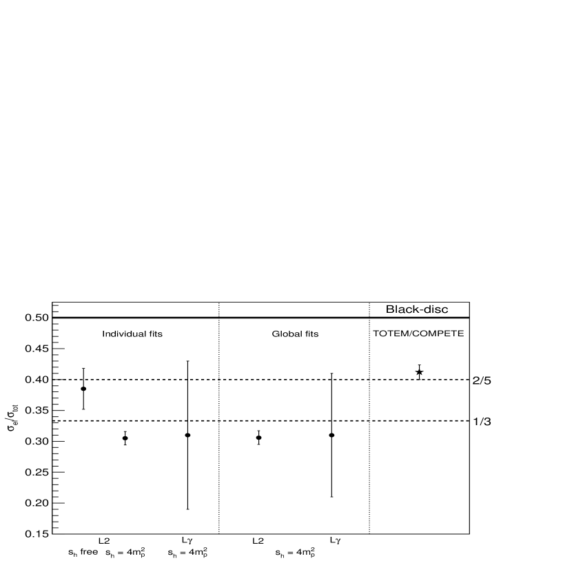
The asymptotic ratios between the elastic and total cross-sections obtained here are displayed in table 6 (individual fits) and table 9 (global fits). Neglecting reference to the $P$ model result, all ratios (individual and global fits) do not exceed 0.430, within the uncertainties (namely the upper uncertainty bounds), indicating, therefore, asymptotic values below 0.5, the black-disk limit. These values within their uncertainties are schematically summarized in figure 10 (including one point to be discussed below).

It may be interesting to note that the TOTEM Collaboration usually displays in their figures an analytical (empirical) fit to the elastic cross section data [10, 11]

$$\sigma_{\mathrm{el}}(s)=11.4-1.52\ln{s}+0.130\ln^{2}{s},$$

which, with our notation in section 3.3.2, equation (15), indicates

$$\beta_{\mathrm{el}}^{\mathrm{TOTEM}}=0.130\ \mathrm{mb}.$$

Now, if we use the 2002 COMPETE result for the total cross section, from table 1, we have

$$\beta_{\mathrm{tot}}^{\mathrm{COMPETE}}=0.3152\pm 0.0095\ \mathrm{mb},$$

and we can infer (for $s\rightarrow\infty$)

$$\frac{\sigma_{\mathrm{el}}}{\sigma_{\mathrm{tot}}}\rightarrow\frac{\beta_{\mathrm{el}}^{\mathrm{TOTEM}}}{\beta_{\mathrm{tot}}^{\mathrm{COMPETE}}}=0.412\pm 0.012.$$ (16)

This point, also displayed in figure 10 (right), corroborates, within all uncertainties, the upper bound 0.430 mentioned above.

Based on figure 10 and tables 6 and 9, we are led to the following conclusions on the asymptotic ratio $\sigma_{\mathrm{el}}/\sigma_{\mathrm{tot}}$.

1. The results from the $L2$ and $L\gamma$ models with $s_{h}$ fixed (individual and global fits) are all consistent within the uncertainties and predict a ratio around 0.3 (fairly below a rational limit 1/3).

2. Within the uncertainties, the results of model $L\gamma$ (individual and global fits) are consistent with the rational limit 1/3, as obtained in previous analyses with this model [38, 39].

3. The result from the $L2$ model with $s_{h}$ free (individual fit) and the estimated ratio from the TOTEM and COMPETE parametrizations are almost consistent within the uncertainties, indicating a ratio above 1/3, possibly, around 0.4 = 2/5.

4. All the results here obtained are consistent with an asymptotic ratio below the black-disk limit and, in terms of rational values, it seems plausible to estimate

$$\frac{1}{3}\lesssim\frac{\sigma_{\mathrm{el}}}{\sigma_{\mathrm{tot}}}\lesssim\frac{2}{5}\quad\mathrm{as\ }s\rightarrow\infty.$$

As previously conjectured by Grau et al. [72] and discussed in [38, 39], this result can be interpreted as a combination of the soft scattering states (elastic and diffractive), giving rise to the black-disk limit. In a formal context, it points towards a saturation of the Pumplim bound [73, 74, 75],

$$\frac{\sigma_{\mathrm{el}}}{\sigma_{\mathrm{tot}}}+\frac{\sigma_{\mathrm{diff}}}{\sigma_{\mathrm{tot}}}\leq\frac{1}{2},$$

where $\sigma_{\mathrm{diff}}$ is the cross-section associated with the inelastic dissociation processes. In this context, our above estimation indicates

$$\frac{1}{10}\lesssim\frac{\sigma_{\mathrm{diff}}}{\sigma_{\mathrm{tot}}}\lesssim\frac{1}{6}\quad\mathrm{as\ }s\rightarrow\infty.$$

At last, we recall that these results and arguments contrast with the asymptotic black-disk scenario predicted in the model-dependent amplitude analysis by Block and Halzen [76].

5 Summary, conclusions and final remarks

We have presented a comparative study on three analytic parametrizations for the hadronic total cross-section, distinguished by their high-energy leading (pomeron) contributions. Including the non-degenerate Reggeon terms for the low and intermediated energy region, the parametrizations have been denoted as models $P$, $L2$ and $L\gamma$. The analytic connection with the $\rho$ parameter has been obtained by means of singly subtracted derivative dispersion relations (DDR), with the corresponding subtraction constant as a free fit parameter.

As regards the practical equivalence between integral dispersion relations and DDR (without the high-energy approximation), we have discussed in appendix A the fundamental role of the subtraction constant. We have also observed that in the COMPETE analysis, reference is made on the use of DDR, but without information on the subtraction constant [31, 32].

Our dataset comprised only $pp$ and $\bar{p}p$ scattering, but covering the energy-region from 5 GeV up to 8 TeV. Individual and global fits to $\sigma_{\mathrm{tot}}$ and $\rho$ data have been addressed and also extensions to $\sigma_{\mathrm{el}}$ data with the corresponding extraction of the asymptotic ratios between $\sigma_{\mathrm{el}}$ and $\sigma_{\mathrm{tot}}$. One important and, presently, yet novel aspect of our analysis is the inclusion in the dataset of all the experimental information presently available at 7 TeV and 8 TeV [8, 9, 10, 11].

Based on the results and discussions presented here, we are led to the following four main conclusions:

1. The data reductions with models $L2$ and $L\gamma$ are strongly dependent on the high-energy-scale factor $s_{h}$.

2. The fit results to $\sigma_{\mathrm{tot}}$ and $\rho$ data with models $P$, the $L2$ ($s_{h}$ free) and $L\gamma$ ($s_{h}$ fixed and $\gamma$ above 2) are all consistent within their uncertainties and with the experimental data up to 7 TeV. However, the data reductions partially underestimate the high-precision TOTEM measurement at 8 TeV.

3. Once compared with the above results, model $L2$ with $s_{h}$ fixed is less consistent with the data and in the case of $s_{h}$ free, the leading high-energy pomeron contribution decreases as the energy increases below $\sqrt{s_{h}}\approx$ 7 GeV.

4. With models $L2$ and $L\gamma$ (degenerate trajectories), the extensions of the parametrizations to fit the $\sigma_{\mathrm{el}}$ data led to asymptotic ratios between $\sigma_{\mathrm{el}}$ and $\sigma_{\mathrm{tot}}$ below the black-disk limit, within the uncertainties. The results favor asymptotic rational limits in the interval 1/3 - 2/5 and points towards a saturation of the Pumplin bound.

It is important to emphasize two contrasting physical pictures present in our results and including the 2002 COMPETE result. For $\sigma_{\mathrm{tot}}$, we have, on the one hand, model $P$ and models $L2$ and $L\gamma$ with $s_{h}=4m_{p}^{2}$ implying in an increasing monotonic pomeron contribution for all values of the energy (above the threshold in the last two cases); on the other hand, model $L2$ with $s_{h}$ free predicting a decreasing pomeron contribution as the energy increases below $s_{h}$. Therefore, in the energy region investigated (above the energy cutoff), two contrasting physical pictures emerge, involving only one model/variant (including the COMPETE result) and all the other three cases. That calls into question whether this decreasing effect in the pomeron contribution has a fundamental theoretical/phenomenological justification or is a consequence of the data reduction. That seems a key issue because, as we have shown (also in [39]), this effect is directly related with the striking agreement of the COMPETE extrapolation with the high-precision TOTEM measurements at 7 TeV and 8 TeV.

In our introduction, we have quoted two questions put in our first work on this subject [37]. Based on the results presented here and in our previous analyses [37, 38, 39], we understand that we have collected enough material to improve the answers to these questions without over interpretations: (1) model $L2$ does not represent a unique solution describing the asymptotic rise of the total cross-section; (2) the available data can as well be statistically described by model $P$ with $\epsilon\approx$ 0.093 (table 2) and by model $L\gamma$ with $\gamma\approx$ 2.3 (tables 5 and 8).

Nonetheless, just answering the two questions, our final conclusion, as already stressed in previous works, is that the rise of the hadronic total cross-section at the highest energies still constitutes an open problem, demanding, therefore, further and detailed investigation. In this respect, we understand that an updated analysis, including all the experimental data currently available and along detailed procedures as those developed by the COMPETE Collaboration (more than ten years ago) can certainly provide new and updated insights on the subject, even before the future experimental data at 13-14 TeV. Moreover, updated model-independent analyses on the rise of the ratio between the elastic and total cross section (as, for example, that developed in [77, 78]), may also shed some light on the subject of asymptotia.

Appendix A Derivative dispersion relations and the subtraction constant

In this appendix, we treat the analytical connection between $\sigma_{\mathrm{tot}}(s)$ and $\rho(s)$ using singly-subtracted derivative dispersion relations (DDR). Specifically, the point is to deduce equations (9) - (14) for $\rho(s)$ from the analytical parametrizations for $\sigma_{\mathrm{tot}}(s)$, equations (4) - (8). Although several aspects of this connection had already been discussed in our previous works [37, 38], some points associated with the practical use of the derivative dispersion relations and the role of the subtraction constant deserve to be stressed. In what follows, after reviewing the main formulas related to integral and derivative dispersion relations (section A.1), we present some critical comments on the practical use of the derivative relations (section A.2).

A.1 Analytic results

For $pp$ and $\overline{p}p$ scattering, analyticity and crossing symmetry allow us to connect $\sigma_{\mathrm{tot}}(s)$ and $\rho(s)$ through the formulas [2]

$$\rho^{pp}(s)\sigma_{\mathrm{tot}}^{pp}(s)=\frac{\textrm{Re}\,F_{+}}{s}+\frac{\textrm{Re}\,F_{-}}{s},$$ (17)

$$\rho^{\bar{p}p}(s)\sigma_{\mathrm{tot}}^{\bar{p}p}(s)=\frac{\textrm{Re}\,F_{+}}{s}-\frac{\textrm{Re}\,F_{-}}{s},$$ (18)

where the even ($+$) and odd ($-$) amplitudes are related to the $pp$ and $\overline{p}p$ amplitudes by

$$F_{\pm}(s)=\frac{F^{pp}\pm F^{\bar{p}p}}{2}.$$ (19)

Dispersion relations have been first deduced in the integral form and in the case of the forward direction the standard once-subtracted integral dispersion relations (IDR) can be expressed by [79, 80]

$$\frac{\textrm{Re}\,F_{+}(s)}{s}\equiv\frac{K}{s}+\frac{2s}{\pi}\,P\int_{s_{o}}^{\infty}ds^{\prime}\left[\frac{1}{s^{\prime 2}-s^{2}}\right]\frac{\textrm{Im}\,F_{+}(s^{\prime})}{s^{\prime}},$$ (20)

$$\frac{\textrm{Re}\,F_{-}(s)}{s}\equiv\frac{2}{\pi}\,P\int_{s_{o}}^{\infty}ds^{\prime}\left[\frac{s^{\prime}}{s^{\prime 2}-s^{2}}\right]\frac{\textrm{Im}\,F_{-}(s^{\prime})}{s^{\prime}},$$ (21)

where $K$ is the subtraction constant and $P$ denotes principal value.

On the other hand, for classes of functions of interest, IDR can be replaced by derivative forms [57, 81, 82, 83, 84, 85, 86], known as derivative dispersion relations (DDR). These may be more useful in some practical calculations, as is the case here with the $\ln^{\gamma}(s/s_{h})$ term for $\gamma$ real. In these formulas, differentiation with respect to the logarithm of the energy occurs in the argument of a trigonometric operator, as in the standard form deduced by Bronzan, Kane and Sukhatme in the high-energy approximation ($s_{0}\rightarrow 0$ in equations (20) and (21)) [86]:

$$\frac{\textrm{Re}\,F_{+}(s)}{s}=\frac{K}{s}+\tan\left[\frac{\pi}{2}\frac{d}{d\ln s}\right]\frac{\textrm{Im}\,F_{+}(s)}{s},$$ (22)

$$\frac{\textrm{Re}\,F_{-}(s)}{s}=\tan\left[\frac{\pi}{2}\left(1+\frac{d}{d\ln s}\right)\right]\frac{\textrm{Im}\,F_{-}(s)}{s},$$ (23)

corresponding, as before, to singly-subtracted DDR, under the high-energy approximation (we shall return to this approximation in section A.2).

In order to implement the calculation, including the logarithm parametrizations, we have used the operator expansion form introduced by Kang and Nicolescu [57] (also discussed in [87]):

$$\frac{\textrm{Re}\ F_{+}(s)}{s}=\frac{K}{s}+\left[\frac{\pi}{2}\frac{d}{d\ln s}+\frac{1}{3}\left(\frac{\pi}{2}\frac{d}{d\ln s}\right)^{3}+\frac{2}{15}\left(\frac{\pi}{2}\frac{d}{d\ln s}\right)^{5}+\ .\ .\ .\ \right]\frac{\textrm{Im}\ F_{+}(s)}{s},$$ (24)

$$\frac{\textrm{Re}\ F_{-}(s)}{s} = -\int\left\{\frac{d}{d\ln s}\left[\cot\left(\frac{\pi}{2}\frac{d}{d\ln s}\right)\right]\frac{\textrm{Im}\ F_{-}(s)}{s}\right\}d\ln s$$ (25)

$$= -\frac{2}{\pi}\int\left\{\left[1-\frac{1}{3}\left(\frac{\pi}{2}\frac{d}{d\ln s}\right)^{2}\right.\right.$$

$$- \left.\left.\frac{1}{45}\left(\frac{\pi}{2}\frac{d}{d\ln s}\right)^{4}-.\ .\ .\ \right]\frac{\textrm{Im}\ F_{-}(s)}{s}\right\}\,d\ln s.$$

Through these two expansions, with the parametrizations defined for $\sigma_{\mathrm{tot}}(s)$, equations (4) - (8), the optical theorem (1), the $\rho$ definition (3) and the above equations (17) - (19), we obtain the analytic results for $\rho(s)$ given by equations (9) - (14) in section 2.2.

A.2 Comments on the practical use of derivative dispersion relations

For our purposes, it is important to note that equations (20) and (21) are not analytically equivalent to equations (22) and (23) due to the high-energy approximation involved. For the functions of interest here, it is possible to obtain an exact DDR result by taking into account the extremes at $s=s_{0}$ after integration by parts. The result, however, introduces an infinite or double infinite series, depending on the assumptions involved. The main point concerns the term associated with the lower limit of the primitive: assuming it to be zero (if the imaginary part of the amplitude vanishes at the threshold $s_{0}=4m_{p}^{2}$), Cudell, Martynov and Selyugin have obtained a single series [88, 89] and without that assumption Ávila and Menon have obtained a double infinite series [90, 91], corresponding therefore to a general expression. This last result can also be put in the form of a single series using sum rules of the incomplete Gamma function, as demonstrated by Ferreira and Sesma [92] (see also [93] for a recent discussion on these representations and further results).

On the other hand, it is also possible to avoid the use of infinite series. The point is to take into account the practical equivalence between the IDR (exact results) and the above DDR (with the high-energy approximation), once the subtraction constant is used as a free fit parameter. This equivalence has been demonstrated by Ávila and Menon [87] and also verified by other authors [88, 94]: the high-energy approximation is absorbed by an effective subtraction constant. Here, we have assumed this strategy, namely we treat $K$ as a free fit parameter. It is important to stress the main point involved: for the functions of interest in amplitude analyses, in order to obtain practical equivalence between IDR and DDR results, the subtraction constant must be employed as a free fit parameter. To take $K=0$ or to neglect it does not guarantee the correct use of derivative relations. In this respect, it is important to note that in the COMPETE analysis, the authors refer to the use of DDR, but there is no information on the subtraction constant [31, 32].

A second fundamental aspect connected with the subtraction constant demands also some comments. In both IDR and DDR, the subtraction constant appears in the form $K/s$, suggesting that its influence (effect) is limited to the low-energy region. That, however, is not the case in global fits to $\sigma_{\mathrm{tot}}$ and $\rho$ data due to the nonlinear character of the data reduction: $K$ as a free parameter is strongly correlated with all the other free parameters involved, including those in the $\sigma_{HE}(s)$ contribution. This effect has been demonstrated and discussed in [95, 96] in the cases of $s^{\epsilon}$ and $\ln^{2}s$ leading contributions; it is also illustrated in our previous analyses with the $\ln^{\gamma}s$ form. (See, for example, table 6 in [39]: the correlation coefficient between $K$ and $\gamma$ is around 0.8.)

At last, it is well known that $\rho$ is in reality a free parameter in fits to the differential cross section data in the region of the Coulomb-nuclear interference. Therefore it does not have the same character of the total cross-section as an effective physical quantity. Moreover, the inclusion of the $\rho$ information in global fits to $\sigma_{\mathrm{tot}}$ and $\rho$ data constraints the rise of the total cross-section. This effect is also related to the subtraction constant due to its correlation with all the fit parameters, as discussed in [38, 39].

Based on the above facts, we understand that individual fits to $\sigma_{\mathrm{tot}}$ data, together with checks on the corresponding predictions for $\rho(s)$ (using DDR), constitute a more adequate procedure than to treat global fits. Despite our focus on the individual fits, global fits are also treated as a complement in Appendix B and referred to in section 4.

Appendix B Global fits to total cross-section and $\rho$ data

In this appendix, we present the results of the global (simultaneous) fits to $\sigma_{\mathrm{tot}}$ and $\rho$ data with the $L2$ and $L\gamma$ models in the case of $s_{h}=4m_{p}^{2}$ fixed. As initial values, we have used once more the central values of the COMPETE results (table 1) and $K$ = 0. The results, obtained through parametrizations (4), (5), (7) and (8) for $\sigma_{\mathrm{tot}}$ and (9), (10), (12), (13) and (14) for $\rho(s)$, are displayed in the second and fourth columns of table 8 and figures 11 and 12. The results of the extensions to $\sigma_{\mathrm{el}}$ data are shown in the third and fifth columns of table 8 and the corresponding asymptotic ratios $\sigma_{\mathrm{el}}$/$\sigma_{\mathrm{tot}}$ in table 9.

Table 8: Results from global fits to $\sigma_{\mathrm{tot}}$ and $\rho$ data and the extensions to $\sigma_{\mathrm{el}}$ data with the $L2$ and $L\gamma$ models in the case of $s_{h}=4m_{p}^{2}$ fixed. Units as in table 1.

$L2$ model $L\gamma$ model $\sigma_{\mathrm{tot}}$ $\sigma_{\mathrm{el}}$ $\sigma_{\mathrm{tot}}$ $\sigma_{\mathrm{el}}$ $a_{1}$ 53.2 $\pm$ 2.1 27.0 $\pm$ 2.8 59.5 $\pm$ 5.8 32.4 $\pm$ 4.3 $b_{1}$ 0.400 $\pm$ 0.018 0.480 $\pm$ 0.038 0.505 $\pm$ 0.058 0.583 $\pm$ 0.042 $a_{2}$ 33.8 $\pm$ 2.0 0 (fixed) 34.1 $\pm$ 2.0 0 (fixed) $b_{2}$ 0.545 $\pm$ 0.013 $-$ 0.547 $\pm$ 0.013 $-$ $\alpha$ 29.88 $\pm$ 0.46 3.68 $\pm$ 0.23 33.4 $\pm$ 1.4 4.70 $\pm$ 0.15 $\beta$ 0.2473 $\pm$ 0.0049 0.0756 $\pm$ 0.0022 0.124 $\pm$ 0.041 0.0382 $\pm$ 0.0010 $\gamma$ 2 (fixed) 2 (fixed) 2.23 $\pm$ 0.11 2.23 (fixed) $s_{h}$ 3.521 (fixed) 3.521 (fixed) 3.521 (fixed) 3.521 (fixed) $K$ 22.6 $\pm$ 6.9 $-$ 40 $\pm$ 13 $-$ DOF 238 104 237 104 $\chi^{2}$/DOF 1.09 1.72 1.08 1.64 $P(\chi^{2})$ 0.163 7.77$\times$10-6 0.184 4.41$\times$10-5 Figure 11 11 12 12

Table 9: Asymptotic results for the ratio $\sigma_{\mathrm{el}}/\sigma_{\mathrm{tot}}$, obtained from the global fits to $\sigma_{\mathrm{tot}}$ and $\rho$ data, with the $L2$ and $L\gamma$ models for $s_{h}=4m_{p}^{2}$ fixed and the extensions to $\sigma_{\mathrm{el}}$, equation (15).

Model Asymptotic Ratio $\sigma_{\mathrm{el}}/\sigma_{\mathrm{tot}}$ $L2$ 0.306 $\pm$ 0.011 $L\gamma$ 0.31 $\pm$ 0.10

Figure 11: Results of the global fits to $\sigma_{\mathrm{tot}}$ and $\rho$ data with the $L2$ model, $s_{h}=4m_{p}^{2}$ fixed and the extensions to the elastic cross-section (table 8, second and third columns).

Figure 12: Results of the global fits to $\sigma_{\mathrm{tot}}$ and $\rho$ data with the $L\gamma$ model, $s_{h}=4m_{p}^{2}$ fixed and the extensions to the elastic cross-section (table 8, fourth and fifth columns).

References

- [1] P. Newman, Recent Experimental Results on Soft Strong Interactions, arXiv:1302.5256 [hep-ex].
- [2] V. Barone and E. Predazzi, High-Energy Particle Diffraction, Spring-Verlag, Berlin, 2002.
- [3] S. Donnachie, G. Dosch, P.V. Landshoff and O. Natchmann, Pomeron Physics and QCD, Cambridge University Press, Cambridge, 2002.
- [4] I.M. Dremin, Phys. Usp. 56 (2013) 3; arXiv: 1206.5474 [hep-ph].
- [5] J. Kašpar V. Kundrát, M. Lokajíček and J. Procházka, Nucl. Phys. B 843 (2011) 84.
- [6] R. Fiore, L. Jenkovszky, R. Orava, E. Predazzi, A. Prokudin, O. Selyugin, Int. J. Mod. Phys. A 24 (2009) 2551.
- [7] G. Matthiae, Rep. Prog. Phys. 57 (1994) 743.
- [8] G. Antchev et al. (The TOTEM Collaboration), Europhys. Lett. 96 (2011) 21002.
- [9] G. Antchev et al. (The TOTEM Collaboration), Europhys. Lett. 101 (2013) 21002.
- [10] G. Antchev et al. (The TOTEM Collaboration), Europhys. Lett. 101 (2013) 21004.
- [11] G. Antchev et al. (The TOTEM Collaboration), Phys. Rev. Lett. 111 (2013) 012001.
- [12] J. Beringer et al. (Particle Data Group), Phys. Rev. D 86 (2012) 010001; http://pdg.lbl.gov.
- [13] R.J. Eden, Rev. Mod. Phys. 43 (1971) 15.
- [14] J. Fischer, Phys. Rep. 76 (1981) 157.
- [15] S.M. Roy, Phys. Rep. 5 (1972) 125.
- [16] A. Martin, in: B. Nicolescu, J. Tran Thanh Van (Eds.), Elastic and Diffractive Scattering at the Collider and Beyond, Editions Frontiìeres, Gif Sur Yvette, 1985, pp. 153 - 163.
- [17] P. Valin, Phys. Rep. 203 (1991) 233.
- [18] M. Froissart, Phys. Rev. 123 (1961) 1053.
- [19] A. Martin, Phys. Rev. 129 (1963) 1432.
- [20] Y.S. Jin, A. Martin, Phys. Rev. 135 (1964) B1375.
- [21] A. Martin, Nuovo Cimento A 42 (1966) 930.
- [22] H. Epstein, V. Glaser, A. Martin, Commun. Math. Phys. 13 (1969) 257.
- [23] L. Lukaszuk, A. Martin, Nuovo Cimento A 52 (1967) 122.
- [24] Ya.I. Azimov, Phys. Rev. D 84 (2011) 056012.
- [25] Ya.I. Azimov, Froissart bounds for amplitudes and cross-sections at high energies, arXiv: 1204.0984 [hep-ph].
- [26] Ya. Azimov, What is the real meaning of the Froissart theorem?, arXiv: 1208.4304 [hep-ph].
- [27] R.J. Eden, P.V. Landshoff, D.I. Olive, J.C. Polkinghorne, The Analytic S-Matrix (Cambridge University Press, Cambridge, 1966).
- [28] R.J. Eden, High Energy Collisions of Elementary Particles, Cambridge University Press, Cambridge, 1967.
- [29] P.D.B. Collins, An Introduction to Regge Theory & High Energy Physics, Cambridge University Press, Cambridge, 1977.
- [30] V.N. Gribov, The Theory of Complex Angular Momenta, Cambridge Monographs on Mathematical Physics, Cambridge University Press, Cambridge, 2003.
- [31] J.R. Cudell et al. (COMPETE Collaboration), Phys. Rev. D 65 (2002) 074024.
- [32] J.R. Cudell et al. (COMPETE Collaboration), Phys. Rev. Lett. 89 (2002) 201801.
- [33] K. Igi and M. Ishida, Phys. Rev. D 66 (2002) 034023; Phys. Lett. B 622 (2005) 286.
- [34] M.M. Block and F. Halzen, Phys. Rev. D 70 (2004) 091901; Phys. Rev. D 72 (2005) 036006.
- [35] K. Nakamura et al. (Particle Data Group), J. Phys. G 37 (2010) 075021.
- [36] G. Aielli et al. (ARGO-YBJ Collaboration), Phys. Rev. D 80 (2009) 092004.
- [37] D.A. Fagundes, M.J. Menon and P.V.R.G. Silva, Braz. J. Phys. 42 (2012) 452; arXiv:1112.4704 [hep-ph].
- [38] D.A. Fagundes, M.J. Menon and P.V.R.G. Silva, J. Phys. G: Nucl. Part. Phys. 40 (2013) 065005; arXiv:1208.3456 [hep-ph].
- [39] M.J. Menon, P.V.R.G. Silva, Int. J. Mod. Phys. A 28 (2013) 1350099, arXiv:1212.5096 [hep-ph].
- [40] U. Amaldi et al., Phys. Lett. B 66 (1977) 390.
- [41] C. Augier et al. (UA4/2 Collaboration), Phys. Lett. B 315 (1993) 503.
- [42] M.M. Block, F. Halzen, Braz. J. Phys. 42 (2012) 465; arXiv:1210.3008 [hep-ph], October 2012.
- [43] D.A. Fagundes, M.J. Menon, P.V.R.G. Silva, Reply to “Commentary on Total Hadronic Cross Section Data and the Froissart-Martin Bound by Fagundes, Menon and Silva”, arXiv:1211.3352 [hep-ph], November 2012.
- [44] R.J. Eden, P.V. Landshoff, Phys. Rev. 136 (1964) B1817.
- [45] A. Donnachie and P.V. Landshoff, Z. Phys. C 2 (1979) 55.
- [46] A. Donnachie and P.V. Landshoff, Nucl. Phys. B 244 (1984) 322.
- [47] A. Donnachie and P.V. Landshoff, Phys. Lett. B 296 (1992) 227.
- [48] R.J.M. Covolan, J. Montanha, K. Goulianos, Phys. Lett. B 389 (1996) 176.
- [49] J.R. Cudell, K. Kang and S.K. Kim, Phys. Lett. B 395 (1997) 311.
- [50] P. Desgrolard, M. Giffon, E. Martynov, E. Predazzi, Eur. Phys. J. C 18 (2001) 555.
- [51] E.G.S. Luna and M.J. Menon, Phys. Lett. B 565 (2003) 123.
- [52] E.G.S. Luna, M.J. Menon, J. Montanha, Nucl. Phys. A 745 (2004) 104.
- [53] W. Heisenberg, Z. Phys. 133 (1952) 65.
- [54] H. Cheng, T.T. Wu, Phys. Rev. Lett. 24 (1970) 1456.
- [55] C. Bourrely, J. Fischer, Nucl. Phys. B 61 (1973) 513.
- [56] L. Lukaszuk, B. Nicolescu, Nuovo Cimento Lett. 8 (1973) 405.
- [57] K. Kang and B. Nicolescu, Phys. Rev. D 11 (1975) 2461.
- [58] M.M. Block, R.N. Cahn, Rev. Mod. Phys. 57 (1985) 563.
- [59] K. Hikasa et al. (Particle Data Group), Phys. Rev. D 45 (1992) S1.
- [60] K. Kang, P. Valin, A.R. White, Nuovo Cimento A 107 (1994) 2103.
- [61] J.R. Cudell, V. Ezhela, K. Kang, S. Lugovsky, N. Tkachenko, Phys. Rev. D 61 (2000) 034019.
- [62] Reference [12], http://pdg.lbl.gov/2012/hadronic-xsections/hadron.html.
- [63] M. Honda et al. Phys. Rev. Lett. 70 (1993) 525.
- [64] R.M. Baltrusaitis et al. Phys. Rev. Lett. 52 (1984) 1380.
- [65] P. Abreu et al. (The Pierre Auger Collaboration), Phys. Rev. Lett. 109 (2012) 062002.
- [66] ROOT Framework, http://root.cern.ch/drupal/; http://root.cern.ch/root/html/TMinuit.html.
- [67] F. James, MINUIT Function Minimization and Error Analysis, Reference Manual, Version 94.1, CERN Program Library Long Writeup D506 (CERN, Geneva, Switzerland, 1998).
- [68] P.R. Bevington and D.K. Robinson, Data Reduction and Error Analysis for the Physical Sciences, McGraw-Hill, Boston, Massachusetts, 1992.
- [69] F. Abe et al. (CDF Collaboration), Phys. Rev. D 50 (1994) 5550.
- [70] N.A. Amos et al. (E710 Collaboration), Phys. Rev. Lett. 68 (1992) 2433.
- [71] C. Avila et al. (E811 Collaboration), Phys. Lett. B 445 (1999) 419.
- [72] A. Grau, S. Pacetti. G. Pancheri., Y.N. Srivastava, Phys. Lett. B 714 (2012) 70; arXiv:1206.1076 [hep-ph].
- [73] J. Pumplin, Phys. Rev. D 8 (1973) 2899.
- [74] J. Pumplin, Physica Scripta 25 (1982) 191.
- [75] U.P. Sukhatme, F.S. Henyey, Nucl. Phys. B 108 (1976) 317.
- [76] M.M. Block, F. Halzen, Phys. Rev. D 86 (2012) 051504.
- [77] D.A. Fagundes, M.J. Menon, Nucl. Phys A 880 (2012) 1; arXiv:1112.5115 [hep-ph].
- [78] D.A. Fagundes, M.J. Menon, in: P.V. Gonçalves et al. (Eds.), XII Hadron Physics, AIP Conf. Proc. 1520, American Institute of Physics, New York, 2013, pp. 297-299; arXiv:1208.0510 [hep-ph].
- [79] M.L. Goldberger, Y. Nambu and R. Oehme, Ann. Phys. (NY) 2 (1957) 226.
- [80] P. Söding, Phys. Lett. 8 (1964) 285.
- [81] V. N. Gribov and A. A. Migdal, Yad. Fiz. 8 (1968) 1002 [Sov. J. Nucl. Phys. 8 (1969) 583].
- [82] J. B. Bronzan, in: Symposium on the Pomeron, Argonne National Laboratory, Report No. ANL/HEP-7327, 1973, p. 33.
- [83] J. D. Jackson, in: R.L. Crawford, R. Jennings (Eds.), Proceedings of the Fourteenth Scottish Universities Summer School in Physics, Phenomenology of Particles at High Energies, Academic Press, London, 1974, pp. 1 - 103.
- [84] J. Fischer and P. Kolář, Phys. Lett. B 64 (1976) 45.
- [85] P. Kolář and J. Fischer, J. Math. Phys. 25 (1984) 2538.
- [86] J. B. Bronzan, G. L. Kane, and U. P. Sukhatme, Phys. Lett. 49B (1974) 272.
- [87] R.F. Ávila and M.J. Menon, Nucl. Phys. A 744 (2004) 249.
- [88] E. Martynov, J.R. Cudell, O.V. Selyugin, Eur. Phys. J. C 33 (2004) S533.
- [89] J.R. Cudell, E. Martynov, O.V. Selyugin, Ukr. J. Phys. 48 (2003) 1272; arXiv:hep-ph/0307254.
- [90] R.F. Ávila and M.J. Menon, in: M. D’Elia et al. (Eds.), Sense of Beauty in Physics - A Volume in Honour of Adriano Di Giacomo, Edizioni Plus - Pisa University Press, Pisa, 2006, pp. 153 - 158; arXiv:hep-ph/0601194.
- [91] R.F. Ávila and M.J. Menon, Braz. J. Phys. 37 (2007) 358.
- [92] E. Ferreira and J. Sesma, J. Math. Phys. 49 (2008) 033504.
- [93] E. Ferreira and J. Sesma, J. Math. Phys. 54 (2013) 033507.
- [94] J.R. Cudell, E. Martynov, O.V. Selyugin, A. Lengyel, Phys. Lett. B 587 (2004) 78.
- [95] R.F. Ávila, E.G.S. Luna, M.J. Menon, Braz. J. Phys. 31 (2001) 567; arXiv:hep-ph/0105065.
- [96] R.F. Ávila, E.G.S. Luna, M.J. Menon, Phys. Rev. D 67 (2003) 054020.