Comparing Poiseuille with 1D Navier-Stokes Flow in Rigid and Distensible Tubes and Networks
Abstract
A comparison is made between the Hagen-Poiseuille flow in rigid tubes and networks on one side and the time-independent one-dimensional Navier-Stokes flow in elastic tubes and networks on the other. Analytical relations, a Poiseuille network flow model and two finite element Navier-Stokes one-dimensional flow models have been developed and used in this investigation. The comparison highlights the differences between Poiseuille and one-dimensional Navier-Stokes flow models which may have been unjustifiably treated as equivalent in some studies.
Keywords: fluid mechanics; Poiseuille; 1D flow; Navier-Stokes; Newtonian fluid; rigid tube; distensible tube; network of tubes; porous media; hemodynamics.
1 Introduction
Poiseuille flow model has been widely used in the earth science and engineering studies for modeling and simulating the flow of Newtonian fluids in networks of rigid tubes which may represent a network of interconnected pipes for oil transportation or a simplified imitation of porous media. The model is naturally extended to include Poiseuille-like flow of time-independent non-Newtonian fluids [1, 2, 3, 4, 5, 6, 7]. Although the 1D Navier-Stokes flow model for elastic tubes and networks is the more popular [8, 9, 10, 11, 12, 13, 14, 15, 16, 17] and normally is the more appropriate one for biological hemodynamic modeling, Poiseuille model has also been used in some studies for modeling and simulating blood flow in large vessels without accounting for the distensibility of the biological networks.
One of the main differences between Poiseuille and 1D flow models for single tube, which also affects the network flow since the individual tubes in the network are subject to the same flow principles as the stand-alone tubes, is that the flow in the first model depends on the pressure difference while in the second model it depends on the actual pressure at the inlet and outlet [18]. This difference is mainly based on the rigidity and distensibility of the flow ducts in these two types of tubes and networks. Another principal difference between Poiseuille and 1D models for network flow, which reflects their complexity and practical relevance and originates from their single tube models, is that Poiseuille is linear and hence it is numerically solved in a single iteration, while the 1D model is nonlinear and hence it requires an iterative process which may cause convergence instabilities leading to compromises associated with considerable numerical errors and approximations.
Apart from the appropriateness of one of these models or the other for a given physical situation (a reason that dictates which model must be used in a specific situation) there are certain practical advantages and disadvantages of Poiseuille and 1D network flow models. In general Poiseuille is easier to implement, moreover it incurs a relatively low computational cost, normally of the order of of memory space where is the number of network nodes, while the 1D is more difficult to implement with a high computational cost of the order of of memory space. This memory cost, associated with the previously-indicated solver iteration requirement, have obvious consequences on the speed of operation and overall performance. The high computational cost of the 1D model in terms of memory space and CPU time can substantially increase by the demand of fine meshing and the use of higher order interpolation.
On the other hand, the 1D model gives more detailed picture as it depicts the flux and pressure fields over the spatial domain inside the tubes; opposite to the Poiseuille model which can only provide the average flow rate in the tubes and the pressure at the junctions. However, the pressure at the interior points of the tubes can be obtained directly for Poiseuille flow due to the linearity of the pressure field; a feature that cannot be replicated in the 1D flow due to the nonlinearity of the pressure field. Another advantage of the 1D Navier-Stokes model is that it can simulate transient flow as well as steady state flow, while the Poiseuille model is basically time-independent and hence any time-dependent feature cannot be directly and dynamically replicated. However, consideration of transient effects in Poiseuille model may be imitated indirectly by the generation of a sequence of time-independent flow frames which represent snapshots of the overall time-dependent process.
2 Poiseuille Model for Single Tube and Network
Poiseuille formula for the flow of laminar, incompressible, axi-symmetric, time-independent, fully-developed flow of Newtonian fluids in rigid cylindrical tubes assuming no-slip-at-wall [19] conditions is given by
| (1) |
where is the volumetric flow rate, is the tube radius, is the pressure drop along the tube, is the fluid dynamic viscosity and is the tube length. This equation can be derived by several methods [1, 4, 5, 20]; most of which are based on the use of Navier-Stokes equation or one of its subsidiaries.
There are several methods for modeling and implementing Poiseuille flow in a network of rigid tubes. The methods are mainly based on imposing a Poiseuille flow condition defined by a constant conductance, as given by Equation 1, on each tube in the network associated with a conservation of flow condition on all junctions of the network, as well as boundary conditions on all the boundary nodes. In the following we briefly describe one of these methods which may be the most straightforward one and is based on imposing pressure boundary conditions.
For a network with nodes, which include all the internal junctions as well as the boundary nodes, the following system of simultaneous linear equations is formed
| (2) |
where is the tubes conductance matrix with dimensions of , is the pressure column vector with dimensions of and is primarily the total flow column vector with dimensions of . The rows of basically represent the relations describing the net volumetric flow rate on the nodes in the network, which, apart from the boundary nodes, sums up to zero due to the incompressibility of fluid with the absence of sources and sinks inside, while the columns represent the nodes of the network. Similarly, the rows of the vector represent the pressure at the nodes while the rows of the vector primarily represent the net flow at the nodes. The pressure drop across each tube is then split into two parts corresponding to the two nodes involved at the two ends of that tube. All the entries in each row of the conductance matrix are set to zero except the ones related to the tubes that are connected to the node represented by that row. By a proper choice of flow signs, the total flow at each internal junction will be added to zero to satisfy the continuity condition and hence the only sources and sinks for the flow are the boundary nodes. For the rows corresponding to the boundary nodes, the boundary pressure conditions are imposed by setting the diagonal entry of the conductance matrix to unity while all the other entries are set to zero with the corresponding entry of the vector being set to the given pressure boundary value of that node.
Poiseuille model for the networks can be validated by testing the satisfaction of Poiseuille formula (Equation 1) on all the tubes of the network given the obtained pressure at the two end nodes of each tube, plus the satisfaction of the boundary conditions on the boundary nodes and the continuity of flow at each junction node which requires that the net flow in each internal node should be added to zero. A consequence of this is that the outflow (sum of volumetric flow rate at outlet boundary nodes) should be equal to the inflow (sum of volumetric flow rate at inlet boundary nodes).
3 1D Model for Single Tube and Network
The one-dimensional model for the time-independent flow of Newtonian fluids in elastic tubes is derived from the following Navier-Stokes system, which is based on the mass and momentum conservation principles
| (3) |
| (4) |
In these equations, is the tube cross sectional area, is the volumetric flow rate, is the axial coordinate along the tube, is the length of tube, ( with and being the fluid local and mean axial speed respectively) is the correction factor for momentum flux, is the fluid mass density, is the local pressure, and is the viscosity friction coefficient usually given by with being the fluid kinematic viscosity defined as the ratio of the dynamic viscosity to the mass density. The model is based on the assumption of a laminar fully-developed flow of incompressible fluids with a tube having a pressure-dependent cross sectional area.
The relation between the pressure and flow rate in elastic tubes is dependent on the constitutive relation that links the local pressure at a certain point along the tube axis to the cross sectional area of the tube at that point. In reference [18] the following two flow relations have been derived based on two different pressure-area constitutive relations
| (5) |
and
| (6) |
In these equations, is the tube unstretched cross sectional area at reference pressure, while and are the cross sectional area at the inlet and outlet respectively. Equations 5 and 6 are based on the following pressure-area constitutive relations respectively
| (7) |
and
| (8) |
where, in the last two equations, is the actual pressure relative to the reference pressure with which the unstretched area in defined, and and are the proportionality coefficients that control the stiffness of the tube.
On multiplying the mass and momentum conservation equations by weight functions and integrating over the solution domain the weak form of the Navier-Stokes flow system can be obtained. This weak form, with suitable boundary conditions, can then be used as a basis for finite element implementation in conjunction with an iterative scheme such as Newton-Raphson method. A detailed account about the finite element formulation is given in references [21, 18].
The system can also be extended to a network of elastic tubes by imposing suitable pressure or flux boundary conditions on all the boundary nodes, and compatibility and matching conditions on all the internal junctions, where the latter conditions are derived from Riemann’s method of characteristics, and mass and energy conservation [22, 16, 21].
The time-independent finite element solution of the 1D model on a network is validated by fulfilling the boundary and matching conditions plus the time-independent analytical solution, as given by Equations 5 and 6, on each individual tube. The validation of the time-independent finite element solution of the 1D model on a single tube is trivial as the numeric solution can be compared directly to the analytic solution with the inspection of the boundary conditions.
4 Comparing Poiseuille and 1D Models for Single Tube
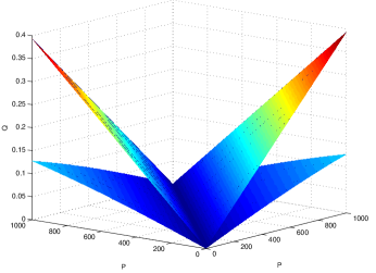
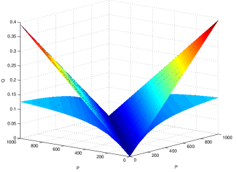
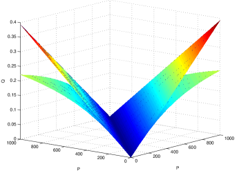
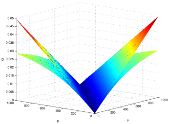
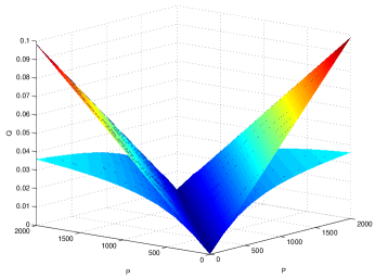
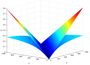
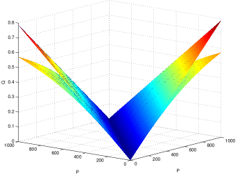
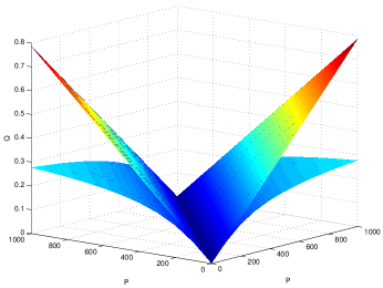
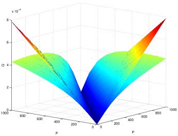
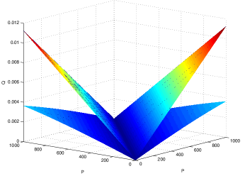
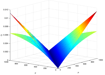
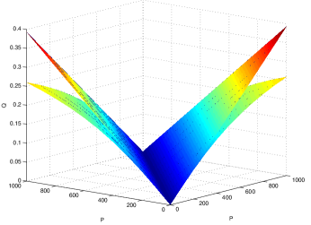
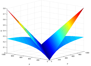
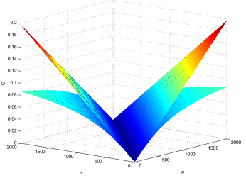
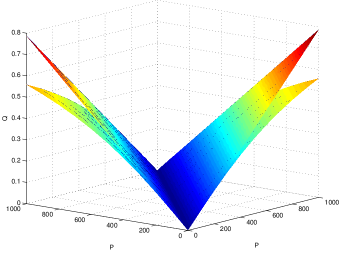
Thorough comparisons between rigid Poiseuille and elastic 1D Navier-Stokes models have been carried out for single tube as part of this study to investigate the effect of various parameters of these two models on the flow behavior. The results of a sample of these comparisons, which represent the two previously mentioned pressure-area constitutive relations, are plotted in Figures 1, 2, 3 and 4. The Poiseuille results shown in these figures are obtained from the analytical solution (Equation 1) while the 1D results are obtained from the analytical expressions (Equation 5 for the first - relation and Equation 6 for the second - relation) with an endorsement by a finite element numeric implementation [18].
As seen, the investigated flow, fluid and tube parameters; which include , , , , pressure regime, , and tube size; have significant effects on the flow conduct of these two models and hence the results are highly dependent on these parameters. It is noteworthy that all these reported results represent qualitative demonstration and hence may not reflect a general trend due to the effect of other parameters which are held constant to investigate the particular dependency. The variation of these parameters is expected to affect the apparent trend in general. We also do not report the values of the other parameters for each one of these cases in detail due to the generality of the current study and the qualitative nature of this demonstration, as well as space limitation and avoiding unnecessary repetition. However, in all these simulations, typical and representative values have been used for the parameters related to the flow, fluid and flow paths, unless stated otherwise. This general conduct has also been followed in the forthcoming investigation of the flow in networks.









5 Comparing Poiseuille and 1D Models for Network
Both - models have been implemented in a finite element network flow computer code as part of this study. However, due to instabilities and convergence difficulties encountered in some cases of the first model which may affect the reliability and generality of the results, we will only present and analyze the results of the second model. This will not affect the generality of this study since a single - model is sufficient to highlight the main issues and draw the conclusions; moreover the generic trends observed from both models are similar in general. In fact the second model is the one which is widely used by the elastic network flow modelers, possibly due to its numerical stability and reliability. The effect of the - model on the Poiseuille versus 1D comparison may deserve a study by itself. It should be remarked that all the network results reported in the current paper, like the single tube results, have been subjected to rigorous checks using the validation criteria outlined in sections 2 and 3.
With regard to the type of networks used in this investigation for Poiseuille and 1D flow simulations, we used fractal-type networks generated by a computer code. The main feature of these networks, which differ in the number of generations and consequently the number of elements which ranges between a few tubes to several thousands, is that they have a fixed branching angle with a constant length to radius ratio; moreover the branching radius transition from one generation of tubes to the next generation is subjected to a Murray-type rule [21], i.e.
| (9) |
where is the radius of the mother tube, is the radius of the th daughter tube, is the number of daughter tubes, and is a constant index. Various networks with different branching angle, length-to-radius ratio, Murray’s index, and number of generations have been used in our investigation. However, most of our networks were generated with and between 2 and 3 with equal-size daughter tubes. A sample of these networks with different number of generations are presented in Figure 5. The reason for using highly regular and symmetric fractal networks is that they, with their simplicity and regularity, reduce the effect of factors related to the complex structure. With the use of these simple fractal networks the flow results will essentially reflect the correlation of the flow with the varied parameters in a simple manner. The use of networks with complex morphology will only obscure the results and complicate the analysis due to the involvement of factors related to the complex geometry and topology of the network.
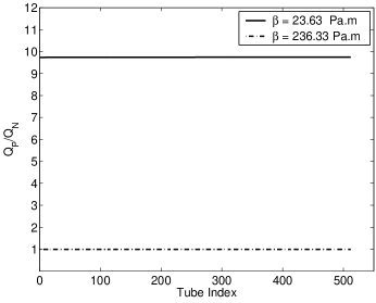
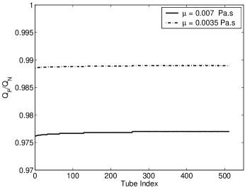
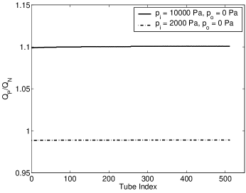
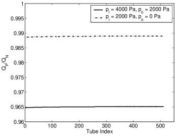
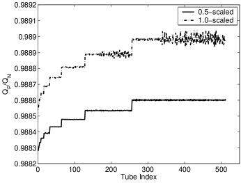
Using these fractal networks in conjunction with the second - model for the 1D Navier-Stokes, a number of Poiseuille and 1D simulations have been conducted using typical network, fluid and flow parameters. In these simulations a typical case in which Poiseuille and 1D produce virtually identical results with , Pa.m, Pa.s, Pa, Pa, and kg/m3 has been used as a reference case. To investigate the effect of the parameters of concern (, , , , , and size) a single parameter was varied at a time from this reference case and a comparison between Poiseuille and 1D was made to identify the effect of that parameter. The method of comparison is based on computing the ratio of the volumetric flow rate between Poiseuille and 1D flow for each tube and plotting this ratio versus tube indices, as seen in Figure 6. Although using the ratio of pressure at each junction node is sensible for making the comparison it has not been used here due to the fact that the pressure at each node for the 1D model is tube-dependent because each tube at a specific junction has its own pressure due to the involvement of Bernoulli energy conservation principle as a matching condition. As for the boundary conditions which were employed in these simulations, a single inlet node belonging to the largest single tube was used to impose an inlet Dirichlet-type pressure boundary condition while all the other boundaries at the other end, which belong to the smallest tubes representing the last generation of the network, were subjected to zero-pressure boundary conditions. However, there is one exceptional case where the outlet pressure was set to a non-zero value to investigate the effect of pressure limits, as seen in Figure 6(e).
On inspecting Figure 6 it can be seen that while and have a significant effect on the 1D flow model as compared to Poiseuille, the other parameters have either moderate or negligible effect. However, this may not be true in general due to the limitation of this study and the number of cases investigated. The use of networks with more complex morphology is expected to introduce other sources of discrepancy between the two models and exacerbate the difference between them.



6 Conclusions
The purpose of this study is to compare Poiseuille model for rigid tubes and networks with the time-independent 1D Navier-Stokes model for elastic tubes and networks based on investigating the effect of the parameters of these two models related to the flow, fluid and flow ducts. The main conclusion of the current investigation is that Poiseuille and 1D models could produce very different results and hence they should not be used interchangeably as it may happened in some studies. The use of one model or the other should be based on the merit of that model and its suitability to capture the physical reality and similar objective considerations, not on convenience and pragmatic factors. Moreover, the results of these models should be assessed relying on independent metrics such as consistency and compliance with experimental observations.
Apart from the main theme of this investigation, it has been observed that for the investigated cases of single tube, all the investigated parameters; which include , , , , , pressure range, and tube size; have significant effects. With regard to the networks, limited in this study to those with fractal character, it has been observed that and have the most sizeable impact. However, the impact of each one of the investigated parameters can be affected by the involvement of other factors such as network topology and geometry. Moreover, other factors are expected to play a significant role in networks with more complex morphology.
Other effects related, for example, to the converging-diverging nature of the flow ducts and non-Newtonian rheology [23, 24, 25], are not considered in this study. These and all other factors should contribute to the complexity of the situation and the departure of the results of Poiseuille and Poiseuille-like models for rigid tubes and networks from the results of the 1D models for distensible tubes and networks.
The comparison presented in the current paper is very general and lacks thoroughness due to specificity of purpose and space limitation. The effect of each one of the investigated parameters, as well as many other aspects not touched in this study such as the effect of morphology of the networks and their statistical distribution, deserve a study on its own.
Nomenclature
| correction factor for axial momentum flux | |
| stiffness parameter in the second pressure-area relation | |
| stiffness parameter in the first pressure-area relation | |
| Murray’s law index | |
| viscosity friction coefficient | |
| fluid dynamic viscosity | |
| fluid kinematic viscosity | |
| fluid mass density | |
| tube cross sectional area | |
| tube cross sectional area at inlet | |
| tube cross sectional area at reference pressure | |
| tube cross sectional area at outlet | |
| conductance matrix | |
| tube length | |
| number of daughter tubes in Murray’s law | |
| local pressure | |
| pressure column vector | |
| inlet pressure | |
| outlet pressure | |
| pressure drop along the tube | |
| volumetric flow rate | |
| total flow column vector | |
| volumetric flow rate of 1D Navier-Stokes model | |
| volumetric flow rate of Poiseuille model | |
| tube radius | |
| radius of daughter tube | |
| radius of mother tube | |
| local axial speed of fluid | |
| mean axial speed of fluid | |
| tube axial coordinate |
References
- [1] A.H.P. Skelland. Non-Newtonian Flow and Heat Transfer. John Wiley and Sons Inc., 1967.
- [2] K.S. Sorbie. Polymer-Improved Oil Recovery. Blakie and Son Ltd, 1991.
- [3] P.H. Valvatne. Predictive pore-scale modelling of multiphase flow. PhD thesis, Imperial College London, 2004.
- [4] T. Sochi. Pore-Scale Modeling of Non-Newtonian Flow in Porous Media. PhD thesis, Imperial College London, 2007.
- [5] T. Sochi; M.J. Blunt. Pore-scale network modeling of Ellis and Herschel-Bulkley fluids. Journal of Petroleum Science and Engineering, 60(2):105–124, 2008.
- [6] T. Sochi. Flow of Non-Newtonian Fluids in Porous Media. Journal of Polymer Science Part B, 48(23):2437–2467, 2010.
- [7] T. Sochi. Computational Techniques for Modeling Non-Newtonian Flow in Porous Media. International Journal of Modeling, Simulation, and Scientific Computing, 1(2):239–256, 2010.
- [8] L. Formaggia; J.F. Gerbeau; F. Nobile; A. Quarteroni. On the coupling of 3D and 1D Navier-Stokes equations for flow problems in compliant vessels. Computer Methods in Applied Mechanics and Engineering, 191(6-7):561–582, 2001.
- [9] N.P. Smith; A.J. Pullan; P.J. Hunter. An Anatomically Based Model of Transient Coronary Blood Flow in the Heart. SIAM Journal on Applied Mathematics, 62(3):990–1018, 2002.
- [10] W. Ruan; M.E. Clark; M. Zhao; A. Curcio. A Hyperbolic System of Equations of Blood Flow in an Arterial Network. SIAM Journal on Applied Mathematics, 64(2):637–667, 2003.
- [11] S.J. Sherwin; V. Franke; J. Peiró; K. Parker. One-dimensional modelling of a vascular network in space-time variables. Journal of Engineering Mathematics, 47(3-4):217–250, 2003.
- [12] S. Urquiza; P. Blanco; G. Lombera; M. Venere; R. Feijoo. Coupling Multidimensional Compliant Models For Carotid Artery Blood Flow. Mecánica Computacional, XXII(3):232–243, 2003.
- [13] G. Pontrelli; E. Rossoni. Numerical modelling of the pressure wave propagation in the arterial flow. International Journal for Numerical Methods in Fluids, 43(6-7):651–671, 2003.
- [14] V. Milišić; A. Quarteroni. Analysis of lumped parameter models for blood flow simulations and their relation with 1D models. Mathematical Modelling and Numerical Analysis, 38(4):613–632, 2004.
- [15] M.Á. Fernández; V. Milišić; A. Quarteroni. Analysis of a Geometrical Multiscale Blood Flow Model Based on the Coupling of ODEs and Hyperbolic PDEs. Multiscale Modeling & Simulation, 4(1):215–236, 2005.
- [16] L. Formaggia; D. Lamponi; M. Tuveri; A. Veneziani. Numerical modeling of 1D arterial networks coupled with a lumped parameters description of the heart. Computer Methods in Biomechanics and Biomedical Engineering, 9(5):273–288, 2006.
- [17] L. Formaggia; A. Moura; F. Nobile. Coupling 3D and 1D fluid-structure interaction models for blood flow simulations. Proceedings in Applied Mathematics and Mechanics, Special Issue: GAMM Annual Meeting 2006 - Berlin, 6(1):27–30, 2006.
- [18] T. Sochi. Flow of Navier-Stokes Fluids in Cylindrical Elastic Tubes. Submitted, 2013.
- [19] T. Sochi. Slip at Fluid-Solid Interface. Polymer Reviews, 51:1–33, 2011.
- [20] T. Sochi. Using Euler-Lagrange Variational Principle to Obtain Flow Relations for Generalized Newtonian Fluids. Submitted, 2013.
- [21] T. Sochi. One-Dimensional Navier-Stokes Finite Element Flow Model. arXiv:1304.2320, 2013.
- [22] L. Formaggia; D. Lamponi; A. Quarteroni. One-dimensional models for blood flow in arteries. Journal of Engineering Mathematics, 47(3/4):251–276, 2003.
- [23] T. Sochi. Non-Newtonian Flow in Porous Media. Polymer, 51(22):5007–5023, 2010.
- [24] T. Sochi. The flow of power-law fluids in axisymmetric corrugated tubes. Journal of Petroleum Science and Engineering, 78(3-4):582–585, 2011.
- [25] T. Sochi. Newtonian Flow in Converging-Diverging Capillaries. International Journal of Modeling, Simulation, and Scientific Computing, 2013. DOI: 10.1142/S1793962313500116.