Phase transitions in the two-dimensional super-antiferromagnetic Ising model with next-nearest-neighbor interactions

Abstract

We use Monte Carlo and Transfer Matrix methods in combination with extrapolation schemes to determine the phase diagram of the 2D super-antiferromagnetic (SAF) Ising model with next-nearest-neighbor (nnn) interactions in a magnetic field. The interactions between nearest-neighbor (nn) spins are ferromagnetic along x, and antiferromagnetic along y. We find that for sufficiently low temperatures and fields, there exists a region limited by a critical line of 2nd-order transitions separating a SAF phase from a magnetically induced paramagnetic phase. We did not find any region with either first-order transition or with re-entrant behavior. The nnn couplings produce either an expansion or a contraction of the SAF phase. Expansion occurs when the interactions are antiferromagnetic, and contraction when they are ferromagnetic. There is a critical ratio $R_{c}=\frac{1}{2}$ between nnn- and nn-couplings, beyond which the SAF phase no longer exists.

One system that has drawn considerable interest recently is the $s=1/2$ super-antiferromagnetic (SAF) Ising model on a square lattice in the presence of a magnetic field Net06 ; Via09 ; Din09 ; Que09 . The model is described by the Ising interactions with a special kind of anisotropy, ferromagnetic $J_{x}$ along $x$ and antiferromagnetic $J_{y}$ along $y$. In the absence of an external field, the ground-state consists of alternating rows of up- and down-spins. Such ordering is known as the SAF order. Also, Onsager’s exact solution for the 2D Ising model applies here Ons44 . There is a critical temperature $T_{c}$, which separates the low-temperature phase with SAF order from the paramagnetic phase. In particular, for $J_{x}=J_{y}=J_{1}$, $T_{c}/J_{1}=2/\ln(1+\sqrt{2})\simeq 2.269$. At $T=0$, an applied external magnetic field $H$ destroys the SAF order at $H_{c}=2J_{1}$, where all the spins become aligned with the field Rot90 .

Figure 1: Energy couplings between neighboring spins of the SAF Ising model.

The phase diagram of the model in the ($H$–$T$) plane has been studied using different approaches. One feature that has caused controversy concerns the re-entrant behavior in the phase diagram found by some authors Cha79 ; Wan97 ; Net06 . Such behavior is absent in other studies Kin75 ; Rot90 ; Din09 ; Via09 ; Que09 . The most recent studies in the literature point to the dismissal of re-entrant behavior. It seems, however, that more scrutiny is needed to clear up this controversy.

Figure 2: Fourth-order cumulant of SAF magnetization versus temperature for several lattice sizes $L$, obtained from Monte Carlo simulations. The curves cross nearly at the same temperature.

The addition of nnn interactions may induce new phases with different orderings and multi-critical points. Consider the case of a closely related system, the 2D Ising model with antiferromagnetic (AF) interactions. In that model, the phase diagram without nnn interactions consists of a second-order critical line separating the low-temperature AF phase from a paramagnetic phase. The inclusion of nnn ferromagnetic interactions reinforces the checkerboard AF order and causes the system to show tricritical behavior. That is characterized by the presence of a tricritical point ($H_{t},T_{t}$) in the phase diagram line where the transition changes from second to first order Lan72 ; Bin80 ; Her83 .

The purpose of this work is to investigate the influence of nnn couplings on the phase transitions of the 2D SAF Ising model in a uniform magnetic field. The Hamiltonian is

$${\cal H}=-J_{x}\sum_{i,j}S^{z}_{i,j}S^{z}_{i+1,j}+J_{y}\sum_{i,j}S^{z}_{i,j}S^{z}_{i,j+1}$$

$$-J_{2}\sum_{i,j}(S^{z}_{i,j}S^{z}_{i+1,j+1}+S^{z}_{i+1,j}S^{z}_{i,j+1})-H\sum_{i,j}S^{z}_{i,j},$$ (1)

where $S^{z}_{i}$ can take the values $\pm 1$. The parameters $J_{x}$ and $J_{y}$ are energy couplings between nn spins along $x$ and $y$, respectively. $J_{2}$ is the coupling between nnn spins, and $H$ the magnetic field.

In this work we assume $J_{x}=J_{y}=J_{1}>0$, whereas $J_{2}$ can be either positive or negative. For simplicity, from here on we use the notation $R=J_{2}/J_{1}$, and set $J_{1}=1$ as the energy unit. Figure 1 shows the energy couplings that appear in Eq. 1.

Figure 3: Crossing temperatures for cumulants of systems of sizes $L$ and $L+2$ versus the ratio $x=L/(L+2)$. Open squares are obtained from MC simulations with $R=-0.2$ and $H=2.0$. The straight line is a numerical fit to the data points.

To determine the phase diagram of the model, we use two different numerical methods, Monte Carlo (MC) Cha86 ; Bin87 ; Lan00 and Transfer Matrix (TM) Nig82 ; Her83 . Both methods have been used in statistical physics problems, especially in Ising-type models. We are interested in the location of the phase boundaries and the nature of the transitions, whether they are of first- or second-order, as well as if re-entrant is observed. Both methods are well-suited to achieve those objectives.

In the present work, we use both methods to determine the phase boundaries. Even though MC is very realible to ascertain the nature of the phases, Bin87 ; Lee90 we elect to use the TM method due mostly to its simplicity. Once the phase boundaries are found by the TM method, little further computational effort is needed to establish their nature Nig82 ; Her83 . We show results for the cases $R=\pm 0.2,\pm 0.4,$ which, as we shall see, will provide the essential features of the phase diagram. We also consider the case $R=0$, which is known Via09 , to check the reliability of our calculations.

In our MC calculations, we use the single-flip Metropolis algorithm Met53 in square lattices of $L\times L$ spins, $8\leq L\leq 128$, with periodic boundary conditions. We divide the lattice into two sub-lattices $A$ and $B$, such that $A$ ($B$) is the set of rows labeled with even (odd) indices. We use even values of $L$ to avoid frustration effects at the edges of the $y$-direction, along which there is AF ordering in the SAF phase.

First, for a given set of the energy parameters and temperature, we let the system equilibrate after $10^{7}$ Monte Carlo steps (MCS). Then we collect the data for each additional configuration generated by a sweep through the lattice. The data are stored in $10^{3}$ bins, each holding up to $10^{4}$–$10^{5}$ sets of data points. This will ensure that the autocorrelation time does not exceed the bin size. The average values in each bin are used to determine the statistical averages and the standard errors. The corresponding error bars are always smaller than the symbols we use in all the graphs that follow.

In addition to the internal energy, specific heat, magnetization, and susceptibility. We also calculate the SAF magnetization fourth-order cumulant, defined by:

$$U_{L}=1-\frac{<M_{s}^{4}>_{L}}{3<M_{s}^{2}>_{L}^{2}}.$$ (2)

The quantities $<M_{s}^{2}>_{L}$ and $<M_{s}^{4}>_{L}$ are the second- and fourth-order moments of the SAF magnetization, $<M_{s}>=\frac{1}{2}<(m_{A}-m_{B})>$. The quantities $<m_{A}>$ and $<m_{B}>$ are the sub-lattice magnetizations, with $<m_{p}>=<\frac{2}{L^{2}}\sum_{i\epsilon p}S_{i}^{z}>$ and $p=A,B$. One of the properties of the fourth-order cumulant, Eq. 2, is that as $T\rightarrow 0$, $U_{L}\rightarrow\frac{2}{3}$, regardless the value of $L$. At criticality, $U_{L}\rightarrow U^{*}$ in the thermodynamic limit Bin81 ; Bin87 ; Ber88 ; Pec91 .

Figure 4: Crossing temperatures for the cumulants of a system of size $L$, with another for size $L+2$, against the ratio $x$. Open squares are from MC simulations with $R=-0.4$ and $H=2.0$, and the straight line is a numerical fit.

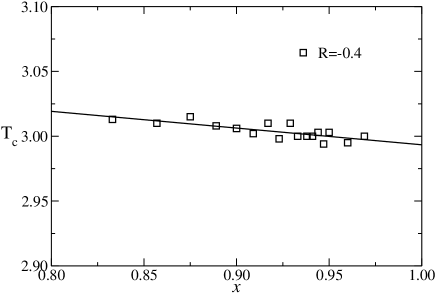
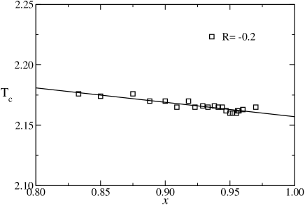
The critical temperature is determined by the intersections of the $U_{L}$ curves for systems of different sizes. As an example, in Fig. 2 we plot the fourth-order cumulant versus temperature for the cases $R=-0.2$, $H_{c}=2.0$, with system sizes $L=8,16,\dots,128$. The curves intersect nearly at the same point. In order to determine the critical temperature at the thermodynamic limit, in Fig. 3 we plot the crossing temperatures for two systems of linear sizes $L$ and $L=L+2$ versus the ratio $x=L/(L+2)$, with the same parameters as in Fig. 2. Note that we use a finer scale for $T$, as compared to the one used in Fig. 2. The open squares are the crossing temperatures. The straight line is a numerical fit to those points, $T_{c}=2.276-0.119\,x$. The extrapolated value at $x=1$, the thermodynamic limit, gives the critical temperature $T_{c}=2.16\pm 0.01$. In Fig. 4 we show the crossing temperatures versus $x$ for $R=-0.4$, and the same parameters in Fig. 3. Here, the straight line $T_{c}=3.122-0.129\,x$ fits the data. In this case, after extrapolation we obtain the thermodynamic value $T_{c}=2.99\pm 0.01$. As can be seen from these figures, the temperature crossings converge fairly rapidly to the thermodynamic value of $T_{c}$. That value can be inferred even when very small lattices are used. We employ this procedure to obtain the critical lines in the $H$–$T$ space. Numerically, it becomes prohibitive time-wise to analyze the region $T<0.2$, since it becomes very difficult to obtain reliable statistics. Hence, in our MC simulations, we only treat cases $T\geq 0.2$.

Figure 5: First correlation length versus magnetic field for infinite-length strips of widths $L=6,8$ lattice spacings obtained from Transfer Matrix method, for the case $R=-0.4$ and $T=0.25$. The curves cross at $H\simeq 3.599945$, indicating a phase transition from the SAF phase to an induced paramagnetic phase.

At $T=0$, however, the model is trivially solvable, so that we can determine the critical temperatures and fields and thus complete the phase diagrams to satisfaction. There are two possible phases which, depending on the applied field, can be the ground-states of the system: the SAF state, with its alternating rows of up- and down- spins, and the induced ferromagnetic (F) state. At sufficient low fields $H$ the SAF state prevails, whereas at very large $H$ all the down-spins are flipped in the direction the field, hence the F state. All other phases, like the AFM-checkerboard or more exotic orderings, will have higher energies than those of the SAF and F states, therefore they can be disregarded. The ground-state energies of the SAF and F states are readily calculated, with results

$$E_{SAF}=-2(1-R)L^{2},$$

$$E_{F}=-(2R+H)L^{2}.$$ (3)

By equating these energies, we determine

$$H_{c}=2-4R,$$ (4)

which is the field strength necessary to align all the spins with the magnetic field without expenditure of energy.

Figure 6: Second correlation length versus magnetic field for the same parameters as in Fig. 5, as obtained from TM method. The absence of crossing indicates that the transition is of second order.

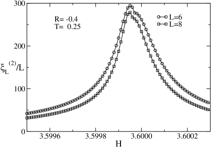
We now proceed to the determination of the phase-diagram of the system by using the TM method Nig82 . In addition to the location of the critical temperatures and fields, the method provides a simple criterion to establish the nature of the transition, whether is of second- or first-order. It relies on two correlation lengths,

$$\xi_{L}^{(\alpha)}=\log^{-1}(E_{0}/E_{\alpha}),$$ (5)

where $\alpha=1$ denotes the first, and $\alpha=2$ the second correlation length. The quantities $E_{0},E_{1},E_{2}$ are the three largest transfer matrix eigenvalues, in descending order, for a strip of width $L$. The critical points are determined using two different lattice sizes ($L$, $M$), using

$$L^{-1}\xi_{L}^{(\alpha)}(H,T)=M^{-1}\xi_{M}^{(\alpha)}(H,T).$$ (6)

We calculate the correlation lengths for infinite strips of widths $L=2,4,\dots,$ and $16$ lattice spacings, with periodic boundary conditions. The final results are extrapolated to $L\rightarrow\infty$.

Figure 7: Critical temperature as a function of the ratio $x$, between the widths $L$ and $L+2$ of infinite-strips. The open circles are from TM results for $R=-0.4$ and $H_{c}=2.0$, whereas the solid line is a numerical fit.

In Fig. 5, we plot the correlation lengths $\xi_{L}^{(1)}$, for two infinite strips of widths $L=6$ and $8$ with $T_{c}=0.25$ and $R=-0.4$. The crossing of the two curves determines the critical field at $H_{c}=3.599945$. We use a similar plot with the second correlation length $\xi_{L}^{(2)}$, to unravel the nature of the transition. Figure 6 shows the second correlation length for strips of widths $L=6$ and $8$. The curves never cross, thus indicating that the transition is of second-order. We have examined the phase diagram with this procedure throughout, and conclude that the transitions are always of second-order for the entire range of parameters, and no re-entrant behavior is ever observed.

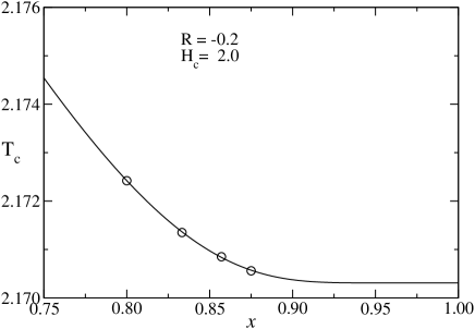
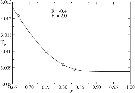
In order to obtain the thermodynamic values of the critical temperatures and fields, in Fig. 7 we plot the critical temperatures $T_{c}$ against the ratio $x=L/M$, $M=L+2$. We choose the same energy parameters as those that were presented in Figs. 3 and 4, to compare with the MC results. The open circles are the numerical results calculated from Eq. 4 for $R=-0.2$ and critical field $H_{c}=2.0$. The solid line is a nonlinear fit using $T_{c}=T_{\infty}+a\exp(-b/(1-x))$. Here, $T_{\infty}=2.1703$, $a=0.06827$, and $b=0.6952$ are the numerically fitted parameters. The quantity $T_{\infty}$ is the extrapolated value for $T_{c}$ in the limit of infinite-width strips. The relative error between $T_{c}$ and $T_{\infty}$ for the largest width ratio used $x=(L/M)=(14/16)$ is about $0.01\,\%$, and less than $0.1\,\%$ for the smallest ratio, $x=(8/10)$. We repeat the above procedure for $R=-0.4$ and $H_{c}=2.0$, and the results are displayed in Fig. 8. Again, the open circles are obtained from Eq. 4. The solid curve is given by the nonlinear fit $T_{c}=3.00887+0.07571\exp(-1.03606/(1-x))$. The extrapolated value for $T_{c}$ at $x=1$ gives the critical temperature of infinite-width strips $T_{\infty}=3.00887$. The relative error between $T_{c}$ and $T_{\infty}$ for the largest widths ratio $x=(10/12)$ is less than $0.005\%$ and about $0.1\%$ for the smallest ratio of strip widths, $x=(4/6)$. The other points of the phase-diagrams can be calculated in a similar fashion. Moreover, even for the smallest ratio, the estimated value for $T_{c}$ is already close to the extrapolated value of the infinite lattice. One should also note the close numerical agreement between $T_{\infty}$ found by the TM method here with the critical temperatures obtained from the MC simulations of Figs. 3 and 4. As will be shown in the following, there is very good agreement between the results of TM and MC in all the phase-diagrams.

Figure 8: Critical temperature vs $x$ for $R=-0.4$ and $H_{c}=2.0$. The open circles are TM results, and the solid line is a numerical fit.

The results from MC and TM methods are shown in Figs. 9 and 10, which depict the critical lines for $R=0,\pm 0.2,\pm 0.4$. The error bars are much smaller than the symbols in the figures and are not shown in the graphs. The critical lines obtained by the two methods show very good quantitative agreement with each other, and also they reproduce the known result Via09 for $R=0$. Data for $R=0$ are shown in the graphs to aid in the visualization of the effects of F ($R>0$) and AF ($R<0$) $nnn$ couplings on the system.

Consider first the critical lines for $R=-0.2$ and $-0.4$, in Fig. 9. The main effect of the nnn AF interactions is the expansion of the SAF region in the phase diagram. Such interactions strengthen the SAF order. Thus it takes larger fields and/or temperatures to break this order.

This is to be contrasted with the case of a simple Ising model with nn AF interactions. There, ferromagnetic nnn interactions reinforce the AF checkerboard order and produce first-order transitions. In our case, reinforcement of the SAF order by nnn AF interactions does not produce first-order transitions.

Figure 9: Critical lines of the model for $R=0$, $-0.2$, and $-0.4$. Dotted lines connect the data points for $R=-0.2$; full lines for $R=-0.4$; and dashed lines for $R=0$. Squares and circles were obtained from MC and triangles from TM, except for the points at $T=0$, which were obtained from Eq. 4.

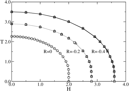
The critical lines for $R=0.2$ and $0.4$ are shown in Fig. 10. There is a shrinkage of the region occupied by the SAF phase as $R$ increases. That is a result of the nnn interactions competing with the local AF couplings, thus weakening the SAF phase. Hence, smaller fields and temperatures are able to destroy the order. The SAF phase region disappears altogether as $R\rightarrow\frac{1}{2}$, which follows from setting $H_{c}=0$ in Eq. 4.

Figure 10: Critical lines for $R=0$, $0.2$, and $0.4$. The nnn couplings are now ferromagnetic and compete with the AF interactions, making it easier to suppress the SAF phase. The symbols have the same meaning as those in Fig. 9.

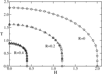
To summarize, we studied the phase transitions of the SAF Ising model in a uniform external magnetic field with nnn couplings on a square lattice. We used two numerical methods, Monte Carlo (MC) and Transfer Matrix (TM) to obtain the critical lines in the ($H$–$T$) plane. We find that all transitions are of second-order and no evidence for re-entrant behavior was observed. Our main results are shown in Figs. 9 and 10. The critical properties of the model are marked by a transition line separating the SAF phase at low temperatures and fields from a paramagnetic phase at high temperatures and fields. The SAF order is reinforced when $R<0$, and depressed when $R>0$, up until the limiting value $R_{c}=\frac{1}{2}$, at which the phase disappears entirely.

We thank FAPERJ (Brazilian agency) for financial support. O.F.A.B. acknowledges support from the Murdoch College of Science Research Program and a grant from the Research Corporation through the Cottrell College Science Award No. CC5737.

References

- (1) M.A. Neto, R.A. dos Anjos, and J.R. de Sousa, Phys. Rev. B 73, 214439 (2006).
- (2) J.R. Viana, M.A. Neto, and J.R. de Sousa, Phys. Lett. A 373, 2413 (2009).
- (3) I.C. Dinola, A. Saguia, and B. Boechat, Phys. Lett. A 373, 1609 (2009).
- (4) S.L.A. Queiroz, Phys. Rev. E 80, 041125 (2009).
- (5) L. Onsager, Phys. Rev. 65, 117 (1944); see also, D.B. Abraham and A. Maciolek, Phys. Rev. E 72, 031601 (2005).
- (6) C. Rottman, Phys. Rev. B 41, 2547 (1990).
- (7) J. Chalupa and M.R. Giri, Solid State Commun. 29, 313 (1979).
- (8) X.-Z. Wang and J.S. Kim, Phys. Rev. Lett. 78, 413 (1997); Phys. Rev. E 56, 2793 (1997).
- (9) J.M. Kincaid and E.G.D. Cohen, Phys. Lett. C 22, 57 (1975); S. Katsura and S. Fijimori, J. Phys. C 7, 2506 (1974).
- (10) D.P. Landau, Phys. Rev. Lett. 28, 449 (1972).
- (11) H.J. Herrmann, Phys. Lett. 100A, 256 (1983).
- (12) K. Binder and D.P. Landau, Phys. Rev. B 21, 1941 (1980).
- (13) M.S.S. Challa, D.P. Landau, and K. Binder, Phys. Rev. B 34, 184 (1986).
- (14) D.P. Landau and K. Binder, A Guide to Monte Carlo Simulation in Statistical Physics (Cambridge University Press, Cambridge, UK, 2000).
- (15) K. Binder and D. Stauffer in Applications of the Monte Carlo Method in Statistical Physics, edited by K. Binder (Springer, Berlin, 1987), p.1.
- (16) P. Nightingale, J. Appl. Phys. 53, 7927 (1982).
- (17) J. Lee and J.M. Kosterlitz, Phys. Rev. Lett. 65, 137 (1990).
- (18) N. Metropolis, A.W. Rosenbluth, M.N. Rosenbluth, A.H. Teller, and E. Teller, J. Chem. Phys. 21, 1087 (1953).
- (19) K. Binder, Z. Phys. B 43, 119 (1981).
- (20) W. Bernreuther and M. Göckeler, Nucl. Phys. B 295, [FS21], 199 (1988).
- (21) P. Peczak, A.M. Ferrenberg, and D.P. Landau, Phys. Rev. B 47, 6087 (1991).