SPIDER VIII – Constraints on the Stellar Initial Mass Function of Early-type Galaxies from a Variety of Spectral Features.
Abstract
We perform a spectroscopic study to constrain the stellar Initial Mass Function (IMF) by using a large sample of early-type galaxies from the SDSS-based SPIDER survey. Clear evidence is found of a trend between IMF and central velocity dispersion (), evolving from a standard Kroupa/Chabrier IMF at km s-1 towards a more bottom-heavy IMF with increasing , becoming steeper than the Salpeter function at km s-1. We analyze a variety of spectral indices, combining gravity-sensitive features, with age- and metallicity-sensitive indices, and we also consider the effect of non solar abundance variations. The indices, corrected to solar scale by means of semi-empirical correlations, are fitted simultaneously with the (nearly solar-scaled) extended MILES (MIUSCAT) stellar population models. Similar conclusions are reached when analyzing the spectra with a hybrid approach, combining constraints from direct spectral fitting in the optical with those from IMF-sensitive indices. Our analysis suggests that , rather than , drives the variation of the IMF. Although our analysis cannot discriminate between a single power law (unimodal) IMF and a low-mass ( M⊙) tapered (bimodal) IMF, robust constraints can be inferred for the fraction in low-mass stars at birth. This fraction (by mass) is found to increase from at km s-1, up to at km s-1. However, additional constraints can be provided with stellar mass-to-light () ratios: unimodal models predict significantly larger than dynamical , across the whole range, whereas a bimodal IMF is compatible. Our results are robust against individual abundance variations. No significant variation is found in Na and Ca in addition to the expected change from the correlation between and .
keywords:
galaxies: stellar content – galaxies: fundamental parameters – galaxies: formation1 Introduction
The formation of stars in a gas cloud is a problem of extraordinary physical complexity, remaining one of the major open problems in modern astrophysics. A way to constrain this fundamental issue is to examine the stellar Initial Mass Function (IMF), i.e. the distribution of the masses of stars at birth. The IMF has critical implications in the framework of galaxy formation and evolution, as it sets the overall mass-scale of galactic systems, controls the intensity of the stellar feedback processes and drives the chemical enrichment abundance patterns.
To date, the IMF can only be directly constrained from star number counts in the disk of the Galaxy. Current observations are consistent with a universal Kroupa/Chabrier-type IMF, i.e. a power-law behaviour at high mass ( M⊙) with a turn-off at lower masses (Kroupa, 2001; Chabrier, 2003), although with a significant uncertainty in the region at masses around a few tenths of M⊙ (see Bastian et al., 2010, and references therein). However, the low-mass portion of the IMF is extremely important because the mass fraction in stars below M⊙ varies from for a Kroupa IMF up to for a Salpeter (1955) IMF, i.e. a large mass fraction of a stellar population is indeed expected in the form of low-mass stars.
An indirect method to study the IMF involves the use of dynamical modelling techniques to constrain the total and stellar mass-to-light ratios of a stellar system. These techniques have been applied to star clusters, favouring a Kroupa-like IMF (see, e.g., Bastian et al, 2006). In early-type galaxies (hereafter ETGs), detailed dynamical modelling of the kinematic properties in a nearby sample revealed a systematic increase in the stellar with galaxy mass (Cappellari et al., 2012a), a result confirmed over a 260-strong sample of ETGs from the ATLAS3D survey (Cappellari et al., 2012c), where the trend is expected to evolve from a Kroupa IMF at low velocity dispersion ( km s-1) towards a Salpeter function at km s-1. Independent dynamical studies have arrived at similar conclusions (see, e.g., Thomas et al., 2011; Wegner et al., 2012; Cappellari et al., 2012a; Dutton, Mendel & Simard, 2012; Tortora et al., 2013). Strong gravitational lensing over galaxy scales can also be exploited to derive stellar especially when the Einstein radius only extends over the central regions, where dark matter does not complicate the issue of transforming total into stellar . Although strong lensing studies of low-mass spheroids rejected a Salpeter IMF (Ferreras et al., 2005, 2008, 2010), recent work covering a wider range of galaxy mass hinted at systematic variations towards higher stellar with increasing mass (Auger et al., 2010; Treu et al., 2010; Barnabé et al., 2011). Hence, both lensing and dynamical studies require a scenario consistent with either a bottom- or a top-heavier IMF than Kroupa/Chabrier in massive ETGs. In fact, a stellar population can have large because of a large fraction of either low-mass stars or remnants of massive stars, and neither dynamical nor lensing modelling is capable of distinguishing between the two (Cappellari et al., 2012a).
A unique opportunity to investigate more directly the IMF is offered by gravity-sensitive features in the integrated light of unresolved stellar populations, as originally proposed by Spinrad (1962). Some of the most discriminant features include the Na I doublet feature at Å (Faber & French, 1980; Schiavon et al., 1997b, hereafter NaI8200), the Wing-Ford FeH band (Wing & Ford, 1969; Schiavon et al., 1997a) at Å, prominent in the atmospheres of low-mass dwarves, as well as the Ca triplet lines at Å(hereafter CaT; see, e.g., Diaz, Terlevich, Terlevich 1989; Cenarro et al. 2003), which are strong in giants, while barely detectable in dwarves. Several other features, mostly related to Na, Ca, and TiO lines, have been also identified in the literature, as potentially useful tools to constrain the dwarf/giant ratio (Conroy & van Dokkum 2012a, Spiniello et al. 2012, hereafter STK12, Smith, Lucey & Carter 2012). Another potentially useful tool is the analysis of (optical-NIR) broad-band colours (Vazdekis et al., 1996, 2012; Ricciardelli et al., 2012). In this respect, ETGs offer a unique opportunity to study the IMF, as they host homogeneous, old, stellar populations, with little amount of dust, allowing for a clean analysis of their stellar content. Nevertheless, this kind of analysis is far from being trivial. All dwarf/giant sensitive features represent a contribution at the level of a few percent to the total galaxy flux, and these features are also sensitive to age, metallicity, as well as abundance ratio of (several) chemical elements. Moreover, NIR features, like NaI8200 and CaT, fall in a spectral region often severely contaminated by sky emission and telluric absorption. These problems have hampered the use of gravity-sensitive features to investigate the IMF for a long time.
The first observational attempts to constrain the giant/dwarf ratio in the IMF were made by Cohen (1978) and Faber & French (1980), towards the centres of M31 and M32, using the NaI8200 feature. Later, Carter et al. (1986) extended the study to a sample of massive ETGs, and found that NaI8200 was enhanced, especially in massive galaxies, with strong radial gradients. These studies concluded in favour of an excess of dwarves (relative to giants) in the galaxy central regions. Opposite conclusions were drawn by Hardy & Couture (1988) and Delisle & Hardy (1992), based on NaI8200A, CaT, and the Wing-Ford band, who explained the radial variation and central strength of these features as a metallicity (rather than IMF) effect. All these early works were in fact plagued by many difficulties, in particular, small sample sizes, low signal-to-noise ratio and resolution of the spectra, or uncertainties in the available stellar population models. The recent availability of dedicated instrumentation and sophisticated reduction techniques has opened up new opportunities to exploit the constraining power of (NIR) IMF-sensitive features, by means of high-quality spectroscopy. Cenarro et al. (2003) proposed a trend towards an excess of low-mass stars in massive galaxies, from a study of the CaT region. More recently, van Dokkum & Conroy (2010, 2011) used the NaI8200A and Wing-Ford band to conclude that the IMF is bottom-heavier than a Kroupa/Chabrier distribution in a sample of eight massive ETGs in the Virgo and Coma clusters. This result has been confirmed, using (theoretical) stellar population models with varying element abundance ratios and a full spectral fitting analysis by Conroy & van Dokkum (2012a), and further extended to a set of 34 ETGs from the SAURON survey (Conroy & van Dokkum, 2012b). At the same time, STK12 and Ferreras et al. (2013, hereafter FLD13) have gone beyond a simple test of universality for the IMF, analyzing large samples of ETGs drawn from the Sloan Digital Sky Survey (SDSS), focusing on Na and TiO spectral features. Remarkably, FLD13 relied on completely independent stellar population models with respect to Conroy & van Dokkum (2012a), using the MIUSCAT (Vazdekis et al., 2012; Ricciardelli et al., 2012) spectrally extended version of the stellar population synthesis models MILES (Vazdekis et al., 2010). Although all these studies favour a non-universal IMF, with more massive ETGs harbouring bottom-heavier distributions than Kroupa/Chabrier, the debate lingers on. In fact, a different picture has been proposed whereby the variation of spectral features with galaxy mass in ETGs is driven by a change of single element (mostly Na and Ca) abundance patterns, rather than an IMF variation (see, e.g., Worthey, Ingermann & Serven, 2011, and references therein). According to this interpretation, for instance, the NaI8200 (CaT) line strength would increase (decrease) with galaxy mass because of an over-(under-)abundance of Na (Ca) relative to Mg in more massive systems. As shown by Conroy & van Dokkum (2012a), a way out to break the degeneracy is by combining spectral features sensitive to IMF with those more sensitive to the abundance of single chemical species. To this effect one has to rely on theoretical models, rather than fully empirical stellar population libraries, to model the impact of variations in both IMF and abundance ratio, over a wide range of wavelength. Therefore, it is important to consider simultaneously a variety of spectral features from different chemical species.
In this paper, we follow this approach. We extend our previous work (FLD13), analyzing stacked spectra of nearby () ETGs with exceptionally high S/N-ratio, spanning a wide range of central velocity dispersion, from to km s-1. As in FLD13, we mainly rely on extended MILES (MIUSCAT) state-of-the-art stellar population models for the analysis. The main novelties of the present contribution are the following: (i) we adopt a wide set of spectral indices (with respect to, e.g., STK12 and FLD13), fitting several TiO, Ca, and Na features simultaneously, to constrain the IMF; (ii) we combine age, metallicity, IMF- and abundance-sensitive features in the analysis; (iii) we use a semi-empirical technique to correct spectral indices to solar-scale, hence allowing for a clean comparison to the base (nearly solar-scaled) models and avoiding to rely completely on theoretical models; (iv) we adopt a wide set of fitting techniques, including a pure spectral index fitting approach, and a hybrid approach, where direct spectral fitting is combined to the constraints from IMF-sensitive indices (as in FLD13); (v) we allow for a wide range of star-formation histories, including one- and two-simple stellar populations (hereafter SSP), as well as exponentially declining star-formation models. All results presented in this work point consistently to a steepening of the IMF with velocity dispersion in ETGs.
The layout of the paper is as follows: Sec. 2 describes the sample of ETGs, drawn from the SDSS-based SPIDER survey. Sec. 2.2 details our stacking procedures. The stellar population models used to analyze the stacks are described in Sec. 3. Sec. 4 presents the spectral indices used in this work, showing their sensitivity to age, metallicity, and IMF. In Sec. 5, we explore the correlation of the targeted spectral indices with abundance ratio. The different fitting methods to interpret the spectra are described in Sec. 6, while results from different fits are discussed in Sec. 7. Sec. 8 shows the ability of the best-fit models, with a varying IMF, to match independent constraints, i.e. mass-to-light ratios and optical-NIR colours. A summary is given in Sec. 9.
2 Data
2.1 Sample
The SPIDER111Spheroids Panchromatic Investigation in Different Environmental Regions (La Barbera et al., 2010a) sample consists of 39,993 nearby (0.05z0.095) ETGs, selected from Data Release 6 of the Sloan Digital Sky Survey (SDSS-DR6; Adelman-McCarthy et al. 2008), as described in La Barbera et al. (2010a, hereafter Paper I). Galaxies are selected to have r-band Petrosian magnitude brighter than , corresponding to an absolute B-band magnitude of , where the separation between the two families of bright and ordinary ellipticals occurs (Capaccioli, Caon & D’Onofrio, 1992; Graham & Guzmán, 2003; Trevisan et al., 2012). The sample covers two orders of magnitude in dynamical mass, from to M⊙ (de la Rosa et al., 2012). Following Bernardi et al. (2003b), we have defined ETGs as bulge-dominated systems (i.e. SDSS attribute , where measures the fraction of galaxy light better fitted by a de Vaucouleurs, rather than an exponential, law), featuring passive spectra within the SDSS fibres (SDSS attribute , where indicates the spectral type of a galaxy based on a principal component analysis). All galaxies have spectroscopy as well as central velocity dispersions, , available from SDSS, and we select those with no spectroscopic warning on (i.e. SDSS attribute set to zero). The spectra, ranging from to Å, are retrieved from SDSS-DR7 (Abazajian et al., 2009), de-redshifted to a common rest-frame and corrected for foreground Galactic extinction (see Paper I). The resulting restframe spectral range varies from – Å, at lowest redshift (), to – Å at the upper redshift limit of the sample (). This spectral coverage gives us the opportunity to study several IMF-sensitive spectral features in ETGs (see Sec. 4), like the Na doublet at Å (Schiavon et al., 1997a, hereafter Na8190), and the Calcium triplet (CaT) at Å (see Cenarro et al. 2001 and references therein). Also, the superb quality of SDSS spectra, with a flux calibration accuracy at the level 222 Adelman-McCarthy et al. (2008) tested the spectrophotometric accuracy of SDSS data by estimating the relative difference between observed and model spectra of white dwarfs. The difference is smaller than from to Å, except for regions possibly affected by interstellar absorption. , is suitable to detect the expected variations – at the level of a few percent – from a varying IMF. We come back to this point at the end of Sec. 2.2.
For the present study, we select the subsample of ETGs with km s-1, as the SPIDER sample becomes significantly incomplete below this limit (see La Barbera et al. 2010b). Following our previous work (Ferreras et al., 2013, hereafter FLD13), we further limit the analysis to objects () with low internal extinction, i.e. a colour excess mag 333 We note that relaxing the threshold in colour excess does not affect our results. For instance, for , the number of objects in each bin changes by a few percent. Since we median-combine the spectra in each bin, the impact of this variation on line strengths is completely negligible (e.g. the equivalent width changes by less than Å in all bins). . The is measured by fitting the SDSS spectrum of each ETG with the spectral fitting code STARLIGHT (Cid Fernandes et al., 2005), assuming a Cardelli, Clayton & Mathis (1989) extinction law (see Swindle et al. 2011, hereafter Paper V, for details). Each spectrum is fitted in the spectral range of to Å, with three different sets of simple stellar population (SSP) models, namely, Bruzual & Charlot (2003, BC03), updated Charlot & Bruzual (often refereed to as CB07), and MILES models (Vazdekis et al., 2010, MI10). Each set of models spans a wide range of ages and metallicities (see Paper V for details). The IMFs used are Scalo (BC03), Chabrier (CB07), and Kroupa (MI10). We estimate by averaging output values from the three STARLIGHT runs 444Runs with different models provide fairly consistent extinction estimates. The mean difference of amounts to about and for BC03-MI10 and CB07-MI10, respectively.. Notice that this procedure is aimed at removing objects with significant internal extinction from the analysis, while not accounting for possible IMF variations within the sample (i.e. the hypothesis we want to test).
Finally, we restrict the sample to spectra with the highest signal-to-noise (S/N) ratio (see Sec 2.2), resulting in a dataset comprising galaxies (i.e. 62% of the original SPIDER catalogue). In addition, for the analysis of the index the sample is further reduced to ETGs as we need to exclude galaxies with redshift , where the index falls close to the red limit of the SDSS spectra.
2.2 Stacked spectra
Dwarf (relative to giant) stars contribute only up to a few percent to the integrated light of galaxies. Hence, constraining the stellar IMF from gravity-sensitive features requires spectra with exquisite signal-to-noise ratio, typically a few hundreds or more (Conroy & van Dokkum, 2012a, hereafter CvD12a). Unfortunately, single SDSS spectra usually do not have such high S/N. For the SPIDER sample, the average S/N over the Na8190 passband ( Å) amounts to (hereafter quoted per Å), ranging from at km s-1 to at km s-1. In order to test for variations of the IMF, we rely on stacked spectra.
As described in FLD13, we have assembled 18 stacked spectra in narrow bins of , over the available range of to km s-1(see Sec. 2.1). The bins have a width of 10 km s-1, except for the last two bins, where, because of the smaller number of galaxies, we adopt the range [260,280], and [280,320] km s-1, respectively. We bin the sample according to , because the underlying stellar populations of ETGs are known to correlate strongly with velocity dispersion (Bernardi et al., 2005). For each bin, we median stack the available spectra, considering only pixels with no SDSS flag raised555i.e. no bad pixels, flat field issues, etc. For details see http://www.sdss.org/dr6/dm/flatFiles/spSpec.html. In order to avoid possible biases related to differences in within the bins, we exclude spectra in the lowest quartile of the distribution in each bin, resulting in a total number of ETGs used to create the stacks. Moreover, in the spectral region of CaT ( Å), we exclude spectra of galaxies at redshift , for which the CaT feature is redshifted beyond the SDSS upper spectral limit of Å. This selection leads to a smaller, but still significant, sample of ETGs used for the stacking at Å. Notice that excluding spectra at over the entire available spectral range does not change significantly the other relevant IMF-sensitive features explored in the present work. For instance, averaging over all stacks, the equivalent width of would change by less than 1 (between the full stacks and those with ). This proves that the EWs of CaT can be meaningfully compared to those of spectral features at bluer wavelengths. Relevant properties of each stack are summarized in Tab. 1, where we report the range of all bins, the number of ETGs per bin, and the median S/N ratio of stacked spectra, computed within the central passband of five representative spectral indices used in this work (Sec. 4). The stacked spectra feature a remarkably high , larger than a few hundreds throughout the whole spectral range. At km s-1, the of the stacks peaks up to a maximum value of () for the IMF-sensitive () spectral feature, at Å ( Å). In addition, in Sec. 5, we probe the effect of variations in on our analysis by further splitting the sample according to , at fixed , we refer the reader to that section for details.
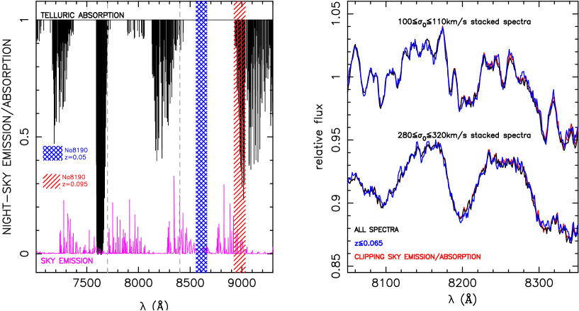
A major source of concern when studying NIR spectral features (e.g. and ) is the possible sky contamination of observed spectra, including telluric absorption and emission lines from the night sky. We performed extensive tests, all of them showing that sky contamination does not affect at all our EW estimates. As an example, Fig. 1 (left panel) plots telluric lines ( from Hanuschik 2006, unpublished) and sky emission lines in the wavelength region of to Å. The red and blue shaded areas mark the observed wavelength range of the Na8190 feature at the lower (; blue) and upper (; red) redshift limit of the SPIDER sample. At , the Na8190 is observed in a region almost unaffected by sky contamination, while at , the feature overlaps with a strong (H2O) telluric band (at Å). The right panel of the same Figure compares the stacked spectra with km s-1 and km s-1 (black curves), to the case where (i) only ETGs at are combined, with Na8190 being virtually unaffected by sky contamination, and (ii) a more “aggressive” stacking approach is adopted, where only flux values more than 1Å away from any telluric line and sky emission are combined. The resulting spectra (not used for the present analysis but for sky contamination tests) show an excellent agreement, with differences at the subpercent level. To obtain a more quantitative estimate of how sky contamination may affect our results, we split the sample into low- and high-redshift bins, with and , respectively. We have produced stacked spectra corresponding to these two intervals for the lowest and highest velocity dispersion bins of our stacks, km s-1 and km s-1, respectively. At highest , the equivalent width 666These equivalent widths are computed on the stacks at their nominal resolution, i.e. no correction is applied to bring them to the same . of the index (see Sec. 4) is Å ( Å) at lower (higher) redshift, while at lowest , the corresponding equivalent widths are and at lower and higher redshift. Consistent with FLD13, we conclude that sky contamination does not affect at all the feature. The same result holds true for the other relevant features. Regarding the index, one may notice that part of this feature always falls within the H2O telluric band, at Å. To test the impact of this on the stacked spectra, we split the sample of ETGs into two redshift bins, with and , respectively. For the – and – km s-1 stacks, we find that a difference of equivalent width between the two intervals of and , respectively, i.e. fully consistent with zero within the errors.
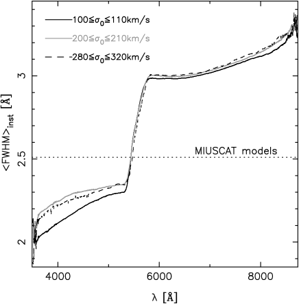
In order to compare stellar population models to stacked spectra of ETGs, we characterize how they are affected by the instrumental resolution of the SDSS spectrograph. For each spectrum, the SDSS pipeline provides the instrumental resolution, , as a function of observed wavelength. We de-redshifted and stacked the curves in the same way as the galaxy spectra. Fig. 2 compares the resulting stacked resolution, , for three representative bins (, , and km s-1). The variation of with reflects the fact that the SDSS resolution is wavelength dependent (see e.g. Bernardi et al. 2003a), increasing from Å for the blue arm of the spectrograph ( Å) to Å for its red arm. Notice that the variation of among stacked spectra is completely negligible ( Å in the blue). For this reason, throughout the present study, we use the average stacked resolution of all spectra in the sample. Notice also that the actual resolution of all stacked spectra analyzed in the present study (given by the SDSS instrumental resolution plus the of each stack 777 Hereafter, with this expression, we mean that the actual resolution of a given spectrum is obtained by adding in quadrature the to the resolution of the SDSS spectrograph. ) is well above that of our reference stellar population models (i.e. the extended MILES models, see below), allowing for an accurate comparison of models and data to be performed.
Finally, we notice that our sample of ETGs is likely contaminated by a small fraction of early spiral systems, i.e., spiral galaxies with a prominent bulge component. As discussed in Paper I, this contamination fraction is about 15, falling to less than 5 for a high quality subsample defined on the basis of visual image classification. We found that restricting the stacking procedure to this high quality selected sample does not lead to any significant change in the relevant spectral indices. For instance, the index changes by less than Å for all stacks. This might be expected because we combine the spectra using the median, instead of the average, and confirms that morphological contamination does not affect at all our conclusions.
| range | median signal-to-noise ratio (Å-1) | |||||
|---|---|---|---|---|---|---|
| (1) | (2) | (3) | (4) | (5) | (6) | (7) |
| – | ||||||
| – | ||||||
| – | ||||||
| – | ||||||
| – | ||||||
| – | ||||||
| – | ||||||
| – | ||||||
| – | ||||||
| – | ||||||
| – | ||||||
| – | ||||||
| – | ||||||
| – | ||||||
| – | ||||||
| – | ||||||
| – | ||||||
| – | ||||||
3 Stellar population models
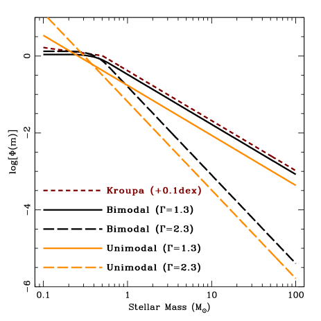
We analyze the spectra of ETGs with the extended MILES (MIUSCAT) stellar population models 888The models are publicly available at http://miles.iac.es/pages/ssp-models/miuscat-models.php. (Vazdekis et al., 2012; Ricciardelli et al., 2012, hereafter MIUSCAT-I, and MIUSCAT-II, respectively), combining CaT (Cenarro et al., 2001) and MILES (Sánchez-Blázquez et al., 2006) with Indo-U.S. empirical stellar libraries over the spectral range Å, at a nominal resolution of Å FWHM (Falcón-Barroso et al., 2011). MIUSCAT models are identical to MILES and CaT models in the spectral ranges covered by these libraries, Å and Å, respectively, while the Indo-U.S. is used to “fill the gap” between MILES and CaT and extend blueward and redward the wavelength coverage of the models (see MIUSCAT-I for details). Notice also that MIUSCAT models rely on solar-scaled isochrones with stellar spectra following the abundance pattern of our Galaxy, i.e. approximately solar-scaled at solar metallicity. The MIUSCAT SSPs cover a wide range of ages, from to Gyr, and seven metallicity bins, i.e. , , , , , . The SSPs are provided for several IMFs. We use here two power-law IMFs, described in Vazdekis et al. (1996), i.e unimodal and bimodal, both characterized by their slope as a single free parameter (see Fig. 3). The bimodal IMFs are similar to the unimodal ones for stars with mass above M⊙, but significantly shallower at lower masses, becoming flat below M⊙. For , the bimodal IMF gives a good representation of the Kroupa IMF, while the unimodal case coincides, for the same slope, with a Salpeter (1955) IMF. The lower and upper mass-cutoff of the IMFs are set to and M⊙, respectively. We refer the reader to appendix A of Vazdekis et al. (2003) for a detailed description of unimodal and bimodal IMFs. For the present study, we interpolate the extended MILES (MIUSCAT) SSPs, for each IMF, over the age (metallicity) range from () to Gyr (), where the models are expected to be safe (see MIUSCAT-I). Younger ages, as well as lower metallicities, than those considered here are not relevant to study our sample of luminous ETGs. The interpolation is done for and steps in age and metallicity, respectively. For bimodal IMFs, we consider the cases , , , , , , , , , . For unimodal IMFs, we restrict the analysis to cases with . At larger slopes, current uncertainties in the modelling of very low Main Sequence stars may impact significantly the synthetic SEDs (see MIUSCAT-I).
4 Spectral indices
Our analysis is mainly based on constraining the IMF by the use of targeted line strengths. We mainly focus on a detailed analysis of the spectral indices, although we also include information from spectral fitting to make the results more robust (as in FLD13, see §§7.5) The use of line strengths brings some well-known drawbacks into the study of unresolved stellar populations. First, indices are defined relative to pseudo-continua, often affected themselves by absorption features. Second, line strengths may reflect the abundance of individual elements in a stellar population, in addition to age, metallicity, and IMF, complicating the interpretation of their variation. On the other hand, spectral indices have the advantage of summarizing the spectral information in a few numbers. In principle, one can define specific indices that efficiently constrain metallicity and age, or – most importantly for this work – single element abundance patterns and the IMF. We select in this paper a variety of spectral indices, bringing the observed line strengths to solar scale by means of their correlations with the abundance ratio (, Sec. 5.2). This has the advantage of allowing for a direct comparison with the expectations from nearly solar-scaled, fully empirical – rather than theoretical – stellar population models (MIUSCAT). In contrast, CvD12a and Conroy & van Dokkum (2012b) adopted a direct spectral fitting approach, using -enhanced stellar population models, based on synthetic stellar spectra to describe the effect of abundance patterns. We notice that most pixels of a galaxy spectrum are sensitive to age, metallicity, and abundance patterns, while only a small number of absorption features are sensitive to the IMF. Therefore, a direct comparison to stellar population models may be driven by differences between models and data, rather than true IMF variations. This further motivates our choice to rely on line strengths, and complement the analysis with the hybrid approach.
We point out that all line indices used for the present analysis are measured at the nominal resolution (i.e. SDSS plus ) of each stack. Since line indices are also sensitive to velocity dispersion – as the broadening of lines changes their contribution to the fluxes measured both in the central and sidebands – we always extract information (e.g. IMF slope) by comparing indices to expectations of stellar population models smoothed to match the resolution of each individual stack. This makes the derived trends (of IMF slope as well as elemental abundances) with independent of resolution. However, and for illustration purposes only, in the figures showing trends of line indices among different stacks, we correct the indices to a reference broadening of km s-1. The correction is done by estimating the variation in each index when smoothing the best-fitting stellar population model to the of a given stack and to , respectively. We note that km s-1corresponds to the central value of the range of our sample, hence this choice of minimizes the correction for all stacks in the figures. Notice that measuring indices at the original resolution of the stack, rather than degrading all stacks to the same maximum value of km s-1, has the advantage of maximizing the information extracted from the data, avoiding the effect of correlated variations among adjacent pixels when smoothing the data. However, to test the impact of resolution on our results, as well as to explore a wider parameter space in the analysis, we smooth both data and models to the same of km s-1, when performing the hybrid approach (Sec. 7.5).
4.1 Selection of spectral features
The list of spectral indices, adopted in this study is assembled as follows.
- IMF-sensitive spectral indices.
-
We have visually inspected the flux ratio of two bimodal SEDs, within contiguous, Å width, spectral windows, looking for IMF-sensitive wavelengths (as, e.g., in figure 9 of MIUSCAT-I). The two SEDs are chosen to have the same age ( Gyr) and (solar) metallicity, with and , respectively. Matching the list of potentially useful wavelengths to existing lists of spectral indices resulted in a list of five IMF-sensitive features 999Notice that the index was also first selected among the IMF-sensitive indices. However, because of its strong sensitivity to , we have decided not to include it in the analysis. Moreover, as discussed by CvD12, the sensitivity of to the IMF is significantly reduced by the fact that a blend partially overlaps with the red pseudo-continuum., namely , , , , and . Here, the is defined as CaT++, following the definition of Cenarro et al. (2001). The definition of spectral indices – mostly based on previous works – is summarized in Tab. 2. Two exceptions are the and features, which are slightly different versions of the index, defined in MIUSCAT-I, and the well-known, Lick-based, molecular band (Trager et al., 1998), respectively. In practice, we have modified the blue (red) pseudo-continua of (), in order to minimize systematic discrepancies between models and data (independent of the IMF). Further details on this issue are given in App. A.
- Abundance-sensitive spectral indices.
-
The list of IMF-sensitive spectral indices is complemented with the and spectral features. These indices, being much more sensitive to Na and Ca abundances than IMF, can be useful tools to break the degeneracy between IMF and abundance ratios (see e.g. CvD12). For instance, by analyzing the diagram vs. NaI (their NaI index being similar to our ), STK12 concluded that both a dwarf-enriched IMF and overabundant are required to match the equivalent widths of a small set of ETGs from the SDSS. A powerful Ca abundance diagnostic is also given by the index (Trager et al., 1998). In fact, the has been recently used by Johansson et al. (2012) to conclude in favour of an underabundance of in ETGs. Unfortunately, we have found that none of our fitting schemes (including the modelling of abundance patterns) is able to produce an acceptable fit to . For this reason, we have excluded this index from the analysis, but for reference, we present a comparison between models and data for this index in Sec. 7.3.1. The definition of abundance-sensitive spectral indices is summarized, together with that of IMF-sensitive indices, in Tab. 2.
- Age-metallicity sensitive spectral indices.
-
In order to account for the well-known variation of age and metallicity with galaxy properties (e.g. Thomas et al. 2005), we also include the , , and spectral indices. The is a modified index, optimized to minimize the age-metallicity degeneracy (Cervantes & Vazdekis, 2009). The is also a very useful age indicator, due to its small sensitivity to , similar to , in constrast to higher-order Balmer lines (Thomas et al., 2004). Finally, we adopt the total metallicity estimator of Thomas et al. (2003a), whose definition removes the residual dependence of the González (1993) spectral index on .
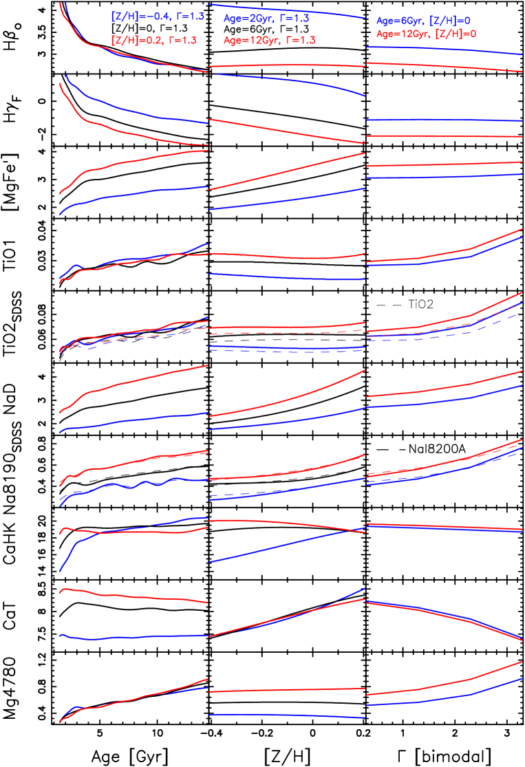
Fig. 4 plots the sensitivity of selected spectral indices to age, metallicity, and IMF. For each index, we show three panels, plotting line strengths of extended MILES (MIUSCAT) SSPs as a function of (from left to right) age, metallicity, and (bimodal) IMF slope, . Each panel shows the model predictions for a small set of simple stellar populations. The extended MILES (MIUSCAT) SSPs have been smoothed to match the wavelength dependent resolution of SDSS (see Sec. 2.2) plus a of km s-1. Both and decrease significantly with increasing age. However, while is essentially independent of metallicity, consistent with its definition (Cervantes & Vazdekis, 2009), tends to decrease with . Both indices (and in particular ) are independent of IMF. is also independent of , increasing with total metallicity, and, to a lesser extent, with age. As expected, all , , , , and show a significant dependence on . The , , , and increase with IMF slope, while exhibits the opposite behaviour. The indices, as well as , are insensitive to metallicity, but tend to increase with age. For (), the latter trend is weaker (similar) to that with . Notice also that has a dependence on age, metallicity, and IMF, very similar to the Lick-based index (dashed curves in the Figure). Regarding , it strongly increases with IMF slope, with a weaker dependence on age and metallicity. The shows a decent sensitivity to IMF, but it strongly increases with both age and metallicity. On the contrary, for age older than Gyr and either solar or super-solar metallicity, the , i.e. the other abundance-sensitive index included in this study, is essentially independent of both age, metallicity, and IMF. The index is constant with respect to age, for SSPs older than a few Gyr, while it depends significantly on metallicity and decreases significantly with increasing IMF slope.
The different sensitivity of all selected spectral indices to age, metallicity, and IMF, makes them a powerful tool to constrain all these parameters simultaneously, as shown in Sec. 7.
An important remark concerns the effect of internal dust on spectral indices. Being a resonant line, can be highly affected by interstellar absorption. This has hampered, so far, its use, in combination with , to constrain the relative contribution of and IMF to gravity-sensitive features. The same issue applies to (see e.g. TMJ11), whose blue pseudo-continuum can be affected by the Na interstellar absorption, leading to overly weak strengths. Notice that our work is virtually unaffected by dust, as the stacked spectra are constructed by removing, ab initio, ETGs with significant amount of reddening. Also, plotting as well as strengths as a function of , for spectra in each bin, does not show any significant correlation.
Another remark is that all our spectral indices are measured within the central diameter aperture of the SDSS fibres, corresponding to a smaller fraction of the effective radius for the more massive galaxies. Radial trends of spectral indices might thus bias our conclusions on the IMF variation with galaxy mass. In App. C we present the trends of some IMF-sensitive indices with effective radius, showing that the aperture effect does not affect our conclusions.
| Index | Units | Blue Pseudo-continuum | Central feature | Red Pseudo-continuum | source |
|---|---|---|---|---|---|
| [Å] | [Å] | [Å] | |||
| Å | – | – | – | Serven+05 | |
| Å | – | – | – | Serven+05 | |
| Å | – | – | – | Trager+98 | |
| mag | – | – | – | Trager+98 | |
| mag | – | – | – | ||
| Å | – | – | – | This work | |
| Å | – | – | – | Cenarro+01 | |
| Å | – | – | – | Cenarro+01 | |
| Å | – | – | – | Cenarro+01 |
5 The effect of
There is a well-known correlation between velocity dispersion and abundance ratio (see, e.g., Trager et al., 2000). This correlation needs to be addressed in our study, to confirm that our trends in the IMF-sensitive spectral indices are not simply caused by the change in . In order to study this issue, we split our sample of ETGs within each bin (see Sec. 2.1), according to . This is done by estimating a proxy of for each galaxy, as detailed in Sec. 5.1. In Sec. 5.2 we present the correlations of indices vs. proxy.
5.1 stacks at fixed
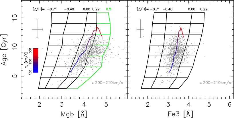
For each ETG, we estimate a proxy of , based on (nearly) solar-scaled extended MILES (MIUSCAT) models. First, we measure the galaxy luminosity-weighted age by spectral fitting the wavelength range from 3900 to 7350 Å 101010The lower limit of Å avoids the bluest part of the SDSS spectral range, which is potentially more affected by small-scale flat-fielding uncertainties, while the upper limit corresponds approximately to the upper limit of the MILES spectral library., with the STARLIGHT fitting code (Cid Fernandes et al., 2005). We feed STARLIGHT with an input list of SSPs, covering a wide range of ages (– Gyr) and metallicities (from to ), assuming a Kroupa IMF. For the given age, we estimate two independent metallicities, and , from the spectral indices and , respectively. This procedure is illustrated in Fig. 5, for galaxies in the km s-1 stack (grey dots). The Figure also plots -Mg and -Fe grids for MILES extended (MIUSCAT) SSPs (Kroupa IMF). While at solar scale both and should coincide, for an -enhanced population the is larger than , as it is actually the case for most data-points. Since the is often larger than the maximum metallicity of the base SSPs (), for each age, we extrapolate the model Mg up to a metallicity of , as shown by the green portion of the grid in the left panel of Fig. 5. We define as solar proxy of , the difference . Notice that for single SDSS spectra estimating ages from spectral fitting, rather than single spectral features (e.g. ), gives a more robust (i.e. less uncertain) age, and thus metallicity, estimate. In fact, the ratio of single (with respect to stacked) SDSS spectra prevents us from obtaining accurate age estimates from alone (with the median equivalent width uncertainty being Å). Large age uncertainties would spread a significant fraction of points at both high and low ages. As seen from the shape of the -Mg grid (Fig. 5), at fixed , young populations do require a larger extrapolation in than older ones, making the proxy estimate more uncertain when the errors in the age are larger. For the stacked spectra, thanks to the high ratio, we estimate the from -based (rather than spectral fitting) ages, as shown in Fig. 5. In practice, we derive the SSP-equivalent age by fitting and equivalent lines with MILES SSPs (Kroupa IMF). Varying the IMF (according to the fitting results of Sec. 7.1) and/or the method to estimate the age (STARLIGHT rather than ), does not change the more than by a few percent 111111On the other hand, the age estimates differ when derived with different methods. For instance, STARLIGHT luminosity-weighted ages are about older than -based, SSP equivalent, ages. This difference implies a vertical offset between the blue-through-red curve and the center of the distribution of grey points in Fig. 5. . The increases systematically for our stacks, from in the lowest bin, up to at highest . This is consistent with the well-known result that the of ETGs increases with (see, e.g., Trager et al., 2000; Thomas et al., 2005).
Since we aim to stack spectra with respect to , an important issue is to establish whether reliable estimates of can be obtained for individual galaxies in our sample. The relevant parameter is the median (per Å) over the passbands of the and spectral features (hereafter ). We find that for individual spectra the ranges from to – quoting the 10-th and 90-th percentiles of the distribution – with a median value of . Notice that the is larger for the Mg and Fe than for the feature, because of the rapid decline of the SDSS spectrograph throughput above Å. We estimate the uncertainty on by comparing estimates of this quantity for galaxies of our sample with repeated observations in SDSS (see Paper I and Paper IV), finding that the error on varies approximately in a linear way with (in the range ), from at , to at . By selecting repeated observations whose spectra have large differences in S/N (), we also find no significant variation in their average (), implying no differential bias in with , and thus with respect to (i.e. among different stacks).
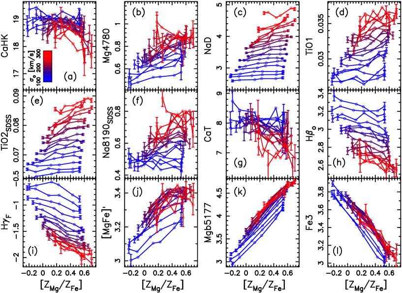
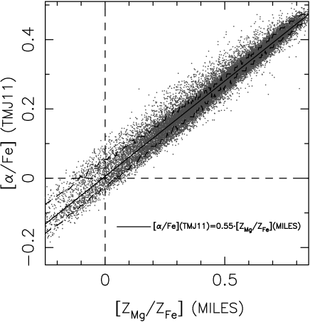
Fig. 6 compares the “presumably-true” 121212The expression “true” refers to estimates obtained from stellar population models taking abundance ratios explicitly into account. with for our sample of ETGs (see Sec. 2.1). The “true” is estimated by comparing the , , and spectral indices of each galaxy to the prescriptions of Thomas, Maraston & Johansson (2011, hereafter TMJ11) -enhanced SSP models (covering a range of age and metallicity). To this effect, we fix the age of TMJ11 models to the luminosity-weighted age measured from STARLIGHT with MILES models, as described above. Hence, both and in Fig. 6 are computed for the same age, but using different models 131313Although the two sets of models differ, one should notice that TMJ11 models are actually based on fitting functions from the MILES stellar library.. Notice the tight relation between and solar proxy, well described by the linear best-fit line in the Figure, with a fitting rms of dex. This small scatter proves that indeed, one can study abundance ratio effects by relying completely on the MILES-based (nearly solar-scaled) proxy. Notice that the relation between and has a slope of about . Hence the of our 18 stacks varies from at lowest , to at highest (see the values reported above).
We stack galaxies according to , considering six bins for each interval. The bins are defined by selecting ETGs (1) below the 10-th percentile, (2) below the 25-th percentile, (3) between the 25-th and 50-th percentiles, (4) between the 50-th and 75-th percentiles, (5) above the 75-th percentile, and (6) above the 90-th percentile of the distribution. For each case, we median-combine the spectra, as described in Sec. 2.2. At fixed , the stacks span a range of (). We use these stacks to study the dependence of our targeted spectral indices on element abundance ratios.
5.2 Correlations with
Fig. 7 plots the variation of the spectral indices as a function of the solar proxy for -enhancement () for all stacked spectra within the 18 bins in . In addition to the indices selected for the IMF study (see above), we also plot and , which enter the definition of (see Sec. 5.1). We point out that all indices are measured at the nominal resolution of the stacks (SDSS plus ). Hence, while the variation of the indices at fixed is not affected by resolution, the variation of indices among different bins is also partly driven by their different velocity dispersion, an effect that we take into account in the analysis (see below).
Most of the targeted spectral indices exhibit clear trends with . This might be due to the dependence of the indices on , but also due to a variation of age, metallicity, IMF, and/or individual element abundances within each bin. The increases with , while shows the opposite behaviour. Notice that this different behaviour is not a mere consequence of the fact that we stacked spectra with respect to , as can change because of either a variation of or . The tight correlation in panels (k) and (i) of Fig. 7, rather, reflect the fact that () anticorrelates with Fe (Mg) abundance (see, e.g., figure 1 of Thomas, Johansson & Maraston 2011). For what concerns the IMF, one can notice that, at fixed , the dynamical range of all IMF-sensitive indices with respect to is much larger than that with at fixed . Hence, the IMF is likely not driving the trends. This result also holds true when removing the effect of age and metallicity, as well as the dependence of line indices on , from the correlations (see below). The panels with , , and show that age and metallicity vary significantly at fixed , in the sense of galaxies with higher -enhancement having older ages (i.e. weaker Balmer lines), as well as higher metallicities (i.e. larger ). This conclusion is based on the fact that, at fixed total metallicity (), both and , as well as , are essentially independent of 141414According to Thomas et al. (2004), and are expected to slightly increase with , while Fig. 7 shows a trend of both indices to decrease with , reflecting a variation in age. .
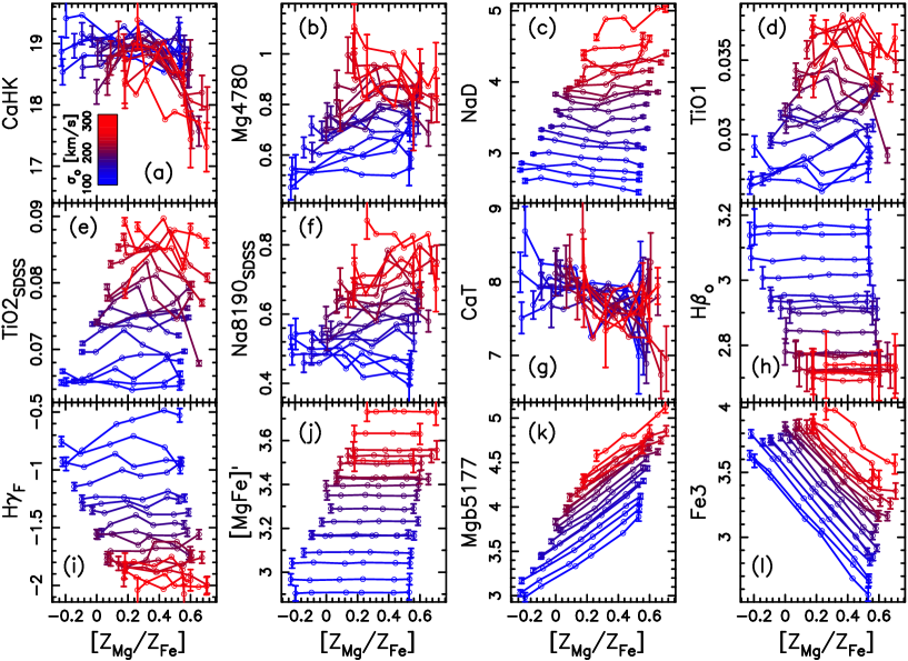
We correct the spectral indices for their dependence on age and metallicity at fixed , as well as their dependence on resolution among stacks with different . The correction procedure estimates age and metallicity from the – diagram for each stack, and then uses those age and metallicity estimates to remove the age/metallicity dependence of each index, for each stack in a given interval. More explicitly, we adopt the following equation:
| (1) |
where is the index line strength for a given stacked spectrum; is the index after correction is applied; is the index value expected for the same stack by fitting its and EWs with extended MILES (MIUSCAT) SSPs having a Kroupa IMF; is the index value predicted for an SSP with a Kroupa IMF, km s-1 (see Sec. 4), and age and metallicity fixed to their average values within the bin. Notice that the quantities are computed by first correcting for nebular emission (see App. B for details). The is computed at the same resolution as , i.e. the SDSS resolution plus the of the given stack. Since is computed at km s-1, Eq. 1 does also correct the trends of Fig. 7 to the same spectral resolution. We point out that the correction does not assume any variation of IMF among stacks, which is the hypothesis to be tested in this paper. Furthermore, as noticed in Sec. 4, the reference value of km s-1is the central value of the range of our stacks, hence minimizing the resolution correction to the indices for all bins. Fig. 8 is the same as Fig. 7 but after applying Eq. 1, i.e. it shows the genuine dependence of the indices on . Most of the trends are weaker than those presented in Fig. 7. In particular, by construction, and do not show any variation with , while does not show any significant correlation with , aside from a few bins (e.g. for the lowest ; where the correction might have been overestimated). For what concerns IMF-sensitive indices, as already noticed above, their variation with is similar, or even larger, at low , implying that is the main driver of IMF variations among stacks. Since the error on is about dex (see Sec. 5), i.e. significantly smaller than the range of dex, our finding is likely not affected by the errors on . In addition, by stacking only galaxies with a higher (), we find consistent trends to those presented in Fig. 8.
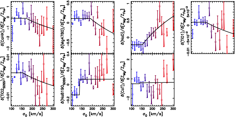
In order to characterize the trends of spectral indices with , we fit them with linear relations, treating index values as independent variables. In Fig. 9, we plot the slopes of the best-fitting relations, , as a function of . For each index line strength, , and each bin, we also compute the rms of the residuals around the best fit . The quantity provides an estimate of the uncertainty in the use of linear relations to interpolate/extrapolate index values to solar abundances (), and is included into the error budget when fitting stellar population models to data (Sec. 6). The figure shows that all indices except , exhibit two regimes with different slopes, featuring a constant slope at low ( km s-1), followed by a correlation with at higher velocity dispersion. This behaviour is traced by the black curves in each panel of Fig. 9. Each curve is obtained by connecting the median slope value at low to a best-fitting power-law relation at higher . For , we notice that our stacking procedure involves fewer spectra (i.e. only those at lower redshift, see Sec. 2.2), making the corresponding trends – hence the slope values in Fig. 9 – not as robust as with other indices. For instance, given the large uncertainty on the slopes for the three highest bins, we cannot exclude that is insensitive to at lowest , with the slope becoming negative at km s-1, as for . The main features of the trends can be summarized as follows.
| model† | model parameters | |
|---|---|---|
| (1) | (2) | (3) |
| TMJ11 | Salpeter IMF; ; Age Gyr; | |
| CvD12 | Chabrier IMF;; Age Gyr; | |
| COE07 | Chabrier IMF; ; Age Gyr; | |
| CER07 | Kroupa IMF; ; Age Gyr; |
TMJ11: Thomas, Maraston & Johansson (2011); CvD12: Conroy & van Dokkum (2012a); COE07: Coelho et al. (2007); CER07: Cervantes et al. (2007).
- Na indices –
-
At low velocity dispersion, the median slopes are negative, i.e. both and tend to decrease with . On the contrary, at high velocity dispersion, the slopes are positive, i.e. the Na indices increase with . The low- behaviour is qualitatively consistent with the predictions of the CvD12 stellar population models, where is expected to affect the continua of both and , causing these indices to decrease with . However, CvD12 models predict a slope of 151515This value refers to CvD12 models with an age of Gyr and Chabrier IMF, smoothed to km s-1. Notice that CvD12 models are computed for . Hence, higher SSPs have higher total metallicity, and the variation of a given index with does also reflect a metallicity variation. Since tends to increase with , one might expect an even steeper slope (i.e. more negative) than that reported above (). , which is significantly different from the value of one obtains for the lowest three bins of (after accounting for the relation between and , see Fig. 6). The same discrepancy exists for where we measure (at lowest ), while CvD12 models predict . Even stronger differences exist when comparing different models, as shown in Tab. 3, where we report the sensitivity of for different stellar population models, namely CvD12, TMJ11, Cervantes et al. (2007, CER07), and Coelho et al. (2007, COE07). We find large differences when comparing different models 161616 Notice that while some difference between models can be expected because different conventions for metallicity are adopted (i.e. either or ), large differences also exist between models adopting the same definition of metallicity (i.e. TMJ11 vs. CER07, and CvD12 vs. COE07).. Moreover, while CvD12, COE07, and CER07, agree qualitatively, in that the weakens as increases, TMJ11 models predict a mild increase with enhancement. Unfortunately, the same model comparison cannot be performed for , as only CvD12 models can be used to make predictions 171717Neither TMJ11 nor CER07 models have the wavelength coverage required to compute . This is not the case for COE07 synthetic models, but for these models the equivalent width of turns out to be negative, in contrast to observations. at Å.
- TiO indices –
-
The slopes change similarly for both indices, from slightly positive at low to negative (on average) for km s-1. Even in this case, large differences exist when comparing different models, where the two TiO indices are expected to be either almost independent (TMJ11); strongly increasing (CER07); mildly increasing (CvD12); or mildly decreasing (COE07) with .
- Ca indices –
-
Both and have slopes consistent with zero at low . The slopes become negative at high for , while for the trend is less clear. Notice that CvD12 models predict both indices to increase with , the same trend being also predicted by COE07 and CER07 models for the index, in contrast to our findings (at both low and high ). For , this discrepancy might also be due to the fact that this index is expected to be affected, for low mass stars, by chromospheric emission fill-in, hampering its modelling.
- –
-
This index mildly increases with at the lowest , consistent with the expected sensitivity to (see Serven et al., 2005), while it decreases with at high . This double-regime behaviour is similar to that of the other indices shown, and indicates that might be sensitive to other elements 181818For instance, using CvD12 models, one finds that the equivalent width of decreases as increases, showing an opposite behaviour to . besides Mg.
The fact that the response of spectral indices to depends on implies that traces different element abundance ratios at different galaxy mass scales. At high , the positive slope of the trends of and might be reflecting a stronger increase in Na abundance with , with respect to other elements. Would this be the case, one might expect a negative slope of Ca indices at high , as the abundance of Na, at fixed Ca abundance, is expected to influence the Ca line strengths through its effect on electron pressure in stellar atmospheres (see e.g. CvD12). While this is indeed the case for , the situation for is less clear (see above)191919 The fact that we do not see an opposite behaviour among slopes of and Na indices at high argues against a picture whereby abundance ratios, rather than IMF, drive variations of Na and Ca line strengths.. In practice, a variation in with , at fixed , might dominate the effect of electron pressure, eventually leading to no correlation among the slopes of Ca and Na indices. On the other hand, at low (relative to high) , the trends with might be reflecting instead the true dependence of the spectral indices with . Regardless of what causes the variation of the slopes, the main point for the present study is that one can use these slopes, for each bin, in order to correct the observed indices to solar abundance ratio (), and compare them with the predictions from (nearly solar-scale) MILES extended (MIUSCAT) models.
6 Fitting procedure
For a given IMF (either bimodal or unimodal), we adopt a multi-index fitting procedure, minimizing the following expression:
| (2) |
where the sum extends over all the selected spectral indices (see Sec. 4), and are the index line strength corrected to =0 and the correction uncertainty, respectively (see Sec. 5.2), is the measurement uncertainty on (reflecting the statistical noise in a stacked spectrum), and is the (extended MILES; MIUSCAT) model line strength, with being either or (see below). The minimization is performed with respect to the model parameters, and for each stack, both observed and model indices are computed at the nominal resolution (SDSS plus ) of a given stacked spectrum. Three different models are considered, namely:
- 1 SSP –
-
The model parameters are the age and metallicity of a single extended MILES (MIUSCAT) SSP. As described in Sec. 3, we consider SSPs covering a wide range of (200150) ages and metallicities. Eq. 2 is minimized over the grid for each value of , and then, for a given choice of the IMF (i.e. bimodal or unimodal), the value of giving the minimum is selected. The procedure is repeated by shifting indices according to their uncertainties ( and ), resulting in a PDF (probability distribution function) for (marginalized in age and metallicity). For the 1SSP fits, we exclude from the fitting, for reasons explained in Sec. 7.1.
- 2 SSPs –
-
The models consists of a linear combination of two extended MILES (MIUSCAT) SSPs, having the same IMF, but different ages and metallicities. The five model parameters are the ages and metallicities of the 2 SSPs plus a mass fraction giving their relative contribution to the linear combination. The minimization is performed by varying the ages and metallicities of the two populations independently, over the same grid as for 1SSP. Since the 2SSP fitting procedure involves a much larger volume of parameter space, we do not iterate the procedure to estimate uncertainties. Instead, we weight each linear combination by , generating a PDF for (marginalized over all other fitting parameters).
- 2 SSPs –
-
The models consist of 2SSP (five free parameters), plus three free parameters describing the abundances of calcium, sodium, and titanium (, , and , respectively). In practice, we replace in Eq. 2 with , where is the sensitivity of a given index to a variation in the abundance of element . Uncertainties on each fitting parameter (and ) are computed as for the 2SSP fits, marginalizing the PDF over all the other fitting parameters. For each index, we consider only the contribution from the dominant element the index is expected to be sensitive to, i.e. for and , for and , and for and . For a given stacked spectrum (i.e. bin), we compute the corresponding ’s by using the publicly available CvD12 models with varying abundance ratios. These models, having a Chabrier IMF, , and an age of Gyr, are smoothed to match km s-1(i.e. the average of our stacks) plus the SDSS resolution. Varying the velocity dispersion in the smoothing does not change significantly the estimates. In Sec. 7.3, we compare the estimates from CvD12 models with estimates from some simple SSPs we create by using different synthesis ingredients from CvD12 (see App. D), finding good consistency. Using CvD12 models, we have explored the sensitivity of spectral indices to the abundance of several individual elements (Ca, C, Mg, Na, N, Si, Ti), by estimating the variation of each index (with respect to the solar scale) caused by a factor of two change in the abundance of each element. All selected indices are found to be at least three times more sensitive to the dominant, than any other, element. For , , and , the choice of a given element as the dominant one is also consistent with the response of Lick indices to single element abundance ratios, as reported by Johansson et al. (2012, see their fig. 1). Notice that the dominant element of is Mg. Since the should reflect directly the Mg abundance, and the indices of our stacks are corrected to , we do not consider the effect of a residual variation in the 2SSP fits.
7 Fitting results
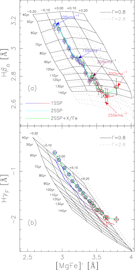
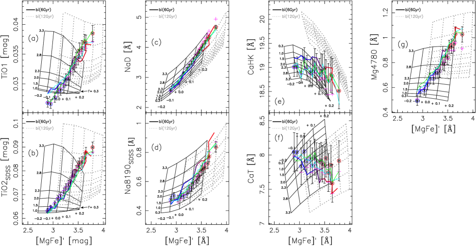
Figs. 10 and 11 compare observed and best-fitting spectral indices for different fitting methods, i.e. , , and models (blue-through-red, cyan, and green curves, respectively). Fig. 10 plots the main age- and metallicity-sensitive indicators, , , and , while Fig. 11 shows abundance- and IMF-sensitive indices. The measured spectral indices, corrected to and reported to a common resolution 202020The correction to km s-1 is performed by computing best-fitting indices at the actual resolution of a given stack and the reference resolution of km s-1. The correction is given by the corresponding difference of line strength values. of km s-1, are plotted as blue-through-red circles. All indices are plotted as a function of (proxy of total metallicity). For each panel in the Figures, the grids correspond to single SSP models, with varying age, metallicity, and bimodal IMF slope, as labelled. The effect of corrections is illustrated by the magenta crosses, showing line strengths when no correction is applied. The corrections are generally mild, shifting data-points (i.e. blue-through-red relative to magenta symbols) within error bars, with the main exception of (see Fig. 11), where the shift at high , towards lower equivalent widths, is significant at more than the 3 level.
To compare the fitting quality among different bins and different fitting methods, we report in Tab. 5, for each fit, the reduced chi-squared statistics, , and the probability, , for the to be larger than the observed value, given the number of degrees of freedom (, with , , and , for , , and , respectively). By definition, lower values of imply less likely best-fitting solutions, with representing a rejection at more than the 2 level for a random normal deviate. In practice, because the models may present small systematic deviations with respect to the data, independent of the relevant stellar population properties (age, metallicity, and IMF), we mainly use the in a relative sense here, i.e. to compare different bins and different methods, as detailed below. We notice that in addition to constraining the IMF slope, different fitting models also give information about the stellar population content (i.e. age and metallicity) of ETGs as a function of . Since our main focus here is that of the stellar IMF, in the following sections we only discuss some general features of the stellar population properties inferred from different fitting schemes, postponing a more detailed analysis to a future paper.
In Secs. 7.1, 7.2, and 7.3 we present the results obtained for , , and models, assuming bimodal IMF models. The case of unimodal IMFs is considered in Sec. 7.4, while Sec. 7.5 presents results of the hybrid approach.
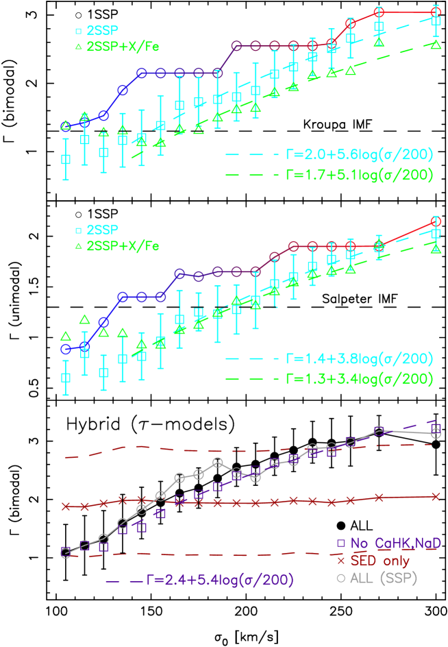
7.1 Bimodal IMFs – fits
Overall, single SSPs reproduce fairly well the relative trends of , , IMF- and abundance-sensitive spectral indices as a function of . As seen from the vs. plot (panel a of Fig. 10), fits yield older ages and higher metallicities with increasing velocity dispersion, in agreement with previous work (e.g. Gallazzi et al. 2006). The IMF slope, , is found to increase, becoming more bottom-heavy at high . This is shown in Fig. 12 (top panel), where we plot the best-fitting , for bi-modal IMFs, as a function of , with the same colour coding, for different bins, as in Fig. 10. The best-fitting increases from (i.e. a Kroupa-like slope) at km s-1 to at km s-1. This IMF trend is consistent with that derived in our previous work (see fig. 4 of FLD13), where we adopted a smaller set of spectral indices, and a different approach to analyze the stacked spectra (see Sec. 7.5): we analyzed the stacks after smoothing all of them to the same of km s-1(rather than keeping them at their original resolution), and no abundance ratio corrections were applied. To further test whether our results are affected by the different resolution of the stacks (see Sec. 4), we repeated the analysis by measuring and fitting line indices after smoothing all spectra and models to km/s, finding negligible differences () in the resulting values of as a function of . Notice that, since slightly decreases with IMF slope (panel a of Fig. 10), a steeper slope for more massive ETGs implies them to have younger ages than expected from a Kroupa/Chabrier IMF. In particular, at highest , for , the highest stacks turn out to have an age of Gyr, i.e. smaller than the age of the Universe, which is not the case when assuming a Kroupa/Chabrier IMF 212121The fact that stellar population models predict ages larger than that of the Universe is known as the age zero-point issue. Although the problem might be solved with a bottom-heavy IMF for high-mass galaxies, it persists for globular clusters, where no evidence exists for a steepening of the IMF. Hence, the zero-point issue still remains as a fundamental aspect to deal with in the modelling of stellar population (e.g. Vazdekis et al. 2001; Schiavon et al. 2002).
A thorough inspection of single panels in Fig. 11 reveals that for IMF- and abundance-sensitive indices some discrepancies exist, at the level of a few ’s, between models and observational data, namely
- –
-
at low (high) , the model line strength of is higher (lower) than the data; i.e., the slope of the - relation is shallower for models than data (see panel a of Fig. 11);
- –
-
the model trend of (panel b) is slightly offset downwards (by ) with respect to the data;
- –
-
at km s-1 the fits give too weak (panel c);
- –
-
the (panel d) is larger for models than data, for most bins; the largest differences amounting to , found for stacks at and km s-1;
- –
-
the (panel f) tends to be weaker in models than data, for all stacks with km s-1; with the largest discrepancies at high , but comparable to the error bars.
Albeit small, all these discrepancies result into probabilities smaller than a few percent for most (13) stacks (see Tab. 5). The discrepancies tend to disappear for models, as discussed in Sec. 7.2. Regarding Balmer lines, we remark that fits include only , i.e. we do not include (see Sec. 6). When only using in the fits, the predicted values are significantly smaller than the observations, as seen in panel (b) of Fig. 10. In other words, the ages inferred from are older (by Gyr) than those derived from alone. The fact that different Balmer lines provide discrepant SSP-equivalent ages is a well-known issue, whose explanation might involve the stronger sensitivity of high-order (relative to ) Balmer lines to (i) (Thomas et al., 2004; Thomas & Davies, 2006), (ii) single element abundance ratios (Serven & Worthey, 2007), and (iii) fraction of young stars (Schiavon, Caldwell & Rose, 2004; Serra & Trager, 2007; Rogers et al., 2010). A detailed analysis of these issues is beyond the scope of the present paper, but we notice that using models (Sec. 7.2) allows us to consistently match both and within error bars, indicating that a model might be too simplistic to describe the data (although we note that the contribution from a second, young, component is not large either, see below).
7.2 Bimodal IMFs – fits
For two SSP models, the fits improve significantly with respect to the case, as seen by comparing cyan () to blue-through-red () curves in Figs. 10 and 11, and by the fact that they give larger values than models (see Tab. 5; with the exception of the lowest , see below). In particular, models fit well the trends of both and with , match and indices at high , give a better description of and on average reproduce better the trends of Ca indices with . On the other hand, some small discrepancies persist:
- –
-
at low ( km s-1), the model predictions of are still too high.
- –
-
a small () average offset remains in , with models having weaker line strength than the data, as in the case;
- –
-
the model is still too high with respect to the observations, but the average difference () is significantly reduced with the use of two populations.
While part of the discrepancy in and that of at low might be explained by a varying abundance ratio (see Sec. 7.3), differences between model and observed indices (e.g. ) might also have an intrinsic origin, reflecting subpercent-level uncertainties in stellar population models, and/or differences between the true shape of the IMF and that assumed in the present analysis (either bimodal or unimodal). We come back to the latter point in Sec. 7.4, when discussing the possibility of discriminating among different IMF shapes.
For what concerns stellar population parameters, for all bins, the best-fit models consist of an old ( Gyr), and a younger population, the latter contributing by less than (in light) to the mixture 222222We notice that the young component is about Gyr old only for the two stacks with km s-1, while in the other cases, excluding the highest bin, it is older than Gyr. At the highest ( km s-1), the young component is Gyr old, but this contributes negligibly, by less than , to the mixture.. Both and fits consistently suggest a significant variation of IMF slope with velocity dispersion. The best-fit changes from at km s-1 to at km s-1 (see top panel of Fig. 12). The shape of the – relation differs significantly between and fitting schemes, with models exhibiting a faster increase with towards a bottom-heavy IMF for more massive systems. At km s-1, the best-fit is , while models give . On the other hand, at km s-1, both and models give compatible values for within error bars. At low , spectral indices are less sensitive to variations in the IMF slope, as seen from the shape of the grids in Fig. 11, hence the larger difference of model predictions for between and fits. The adoption of different stellar population mixtures will therefore affect significantly the inferred values in this regime. In contrast, at high (i.e. ), spectral indices are strongly sensitive to IMF variations, and the constraints on appear more robust with respect to the other stellar population ingredients. In summary, for the purpose of the present work, the main conclusion here is that models plus a varying IMF reproduce well the variation of all spectral indices with , and the quality of the fits does not change significantly with , as proven by comparing values among different bins (see Tab. 5), with the exception of the three lowest bins ( km s-1), where a small variation of single element abundances might be required (see Sec. 7.3).
Following our previous work (FLD13), we model the trend of with with the relation:
| (3) |
where and are obtained by a least-squares fitting procedure to the data, with as dependent variable in the fit. The uncertainties on and are bootstrap errors, reflecting the uncertainties on . Notice that the fit is restricted to stacks with km s-1, where a significant variation of IMF slope with velocity dispersion is detected. The values of and , for as well as for other fitting methods, are summarized in Tab. 4. Notice that, considering the quoted errors, the best-fitting value of () is larger than zero at a level, reflecting the fact that our data strongly support an increase of IMF slope with velocity dispersion in ETGs.
| method | ||
|---|---|---|
| (1) | (2) | (3) |
| bimodal, | ||
| bimodal, | ||
| unimodal, | ||
| unimodal, | ||
| bimodal, hybrid |
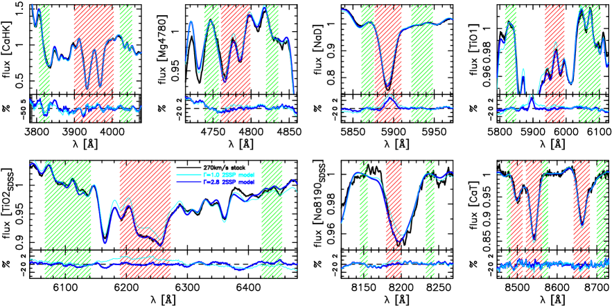
Fig. 13 shows, in wavelength, rather than index–index, space, the main conclusion of the present work, namely that high-mass ETGs are on average better fit by an IMF that is more bottom heavy than the standard Kroupa-like case. The Figure compares the stacked spectrum at km s-1 with the best-fitting model (blue) and a best-fitting model obtained by assuming a IMF, the latter being representative of low-mass ETGs (see top panel of Fig. 12). The comparison is shown for different spectral windows where IMF- and abundance-sensitive spectral indices are defined. Notice that a high () gives the best fit to all relevant features 232323Notice that, in contrast to the indices, the observed spectrum in Fig. 13 is not corrected to solar-scale, which might explain some small discrepancies between models and data in the Figure (e.g., in the though of the line). , i.e. Na and lines, and in particular the observed spectrum in the spectral range, making this feature an extremely useful tool to constrain the IMF (in agreement with STK12).
| range | () | ||
|---|---|---|---|
| (1) | (2) | (3) | (4) |
| – | |||
| – | |||
| – | |||
| – | |||
| – | |||
| – | |||
| – | |||
| – | |||
| – | |||
| – | |||
| – | |||
| – | |||
| – | |||
| – | |||
| – | |||
| – | |||
| – | |||
| – | |||
7.3 The role of individual abundance patterns
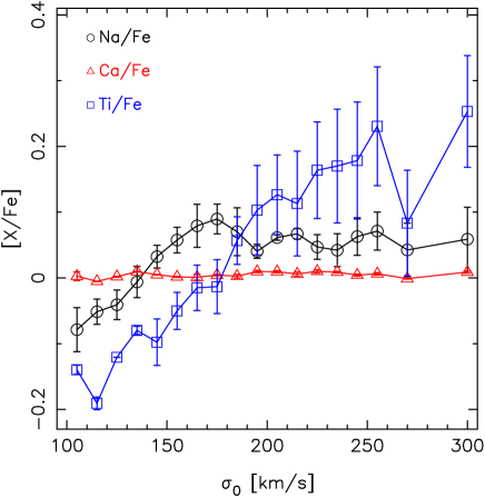
Comparing the cyan and green curves in Fig. 11, one can see that the overall quality of the fits to our targeted spectral indices does not improve significantly when allowing for an individual variation of Ca, Na, and Ti abundance patterns. In fact, for most bins, the probability values are lower for than models (see Tab. 5). On the other hand, looking at TiO features alone, one can notice an improvement with respect to the case, in that models match better at the lowest ( km s-1), as well as at high (in particular around km s-1). The improved matching of is due to the fact that, according to CvD12 models 242424This different sensitivity of and to is qualitatively consistent with the predictions of the TMJ11 models. , is slightly more sensitive to than . Hence, by lowering , one decreases the model more than , allowing both observed indices to be matched simultaneously. This point is illustrated in Fig. 14, where the best-fit abundance ratios, , , and are shown as a function of . We point out that, since spectral indices have been corrected to (see Sec. 5.2), the , , and estimates in Fig. 14 do not reflect true abundance ratios in different bins, but should rather be interpreted as residual abundances, i.e. not accounted for by the correlation of single element abundances with , and the fact that increases with . Another caveat is that we rely on a given set of theoretical models (CvD12) to infer , , and , although we also explore the effect of using our own simple synthetic SSPs (see App. D) partly based on different ingredients to the CvD12 models (see below). For these reasons, our conclusions on individual abundance ratios should be considered on a qualitative basis.
- Ti abundances –
-
The is found to increase with , changing from negative ( dex) at the lowest to positive for km s-1. Notice that at km s-1, the error bars for are very small (less than a few percent), reflecting the fact that a negative value of is required to reduce the discrepancy between model and observed strength for the lowest velocity dispersion stacks. At high , the becomes positive, as increases, producing a better match to the observed . Notice, in fact, that peaks at km s-1 (Fig. 14), where the models differ the most from the data (see panel of Fig. 11). The error bars on are large at km s-1, meaning that a deviation of Ti abundance from solar scale is only marginally significant for massive systems.
- Na abundances –
-
The also increases with , varying by about dex from to km s-1. This amount of variation is far smaller than that recently reported by CvD12b, who found that can be as high as 1 dex for ETGs in the SAURON sample. Notice that this is not necessarily in disagreement with our findings. In fact, the feature is not covered by the observed spectra of CvD12b, with the being inferred indirectly by the authors because of its effect on the free electron pressure in stellar atmospheres. Also, as noticed above, our best-fit abundance ratios should be considered as residual (with respect to ), rather than absolute estimates. The effect of varying on Na indices is illustrated in Fig. 15 (top panel), where is plotted against . We also show the expected effect of varying by dex, when using (i) CvD12 models with a Chabrier IMF, solar metallicity, and an age of Gyr (blue arrow); (ii) our synthetic SSP, with a Kroupa IMF, solar metallicity, and age of Gyr (red arrow); (iii) the same SSP but for a Salpeter IMF (orange arrow). We refer the reader to App. D for details on how our synthetic SSPs are created. Notice the remarkable agreement between CvD12 and our-SSP predictions for a Chabrier/Kroupa IMF. Increasing makes both and to increase along a direction which is either steeper (Chabrier/Kroupa) or similar (Salpeter SSP) to the observed – trend. This indicates that disentangling the effect of IMF and is in general very difficult, and one actually needs a multi-index approach, based on indices from different species, as in the present work. We emphasize that a significant variation of with alone (after correcting for the trends) appears to be ruled out by our data, as the fits reproduce well the – trend, as well as the other index- trends.
- Ca abundances –
-
The best-fit is very close to zero for all stacks, with small error bars throughout the full range. The reason of this behaviour is illustrated in Fig. 15 (bottom panel), where is plotted as a function of . The effect of decreasing Ca abundance by a “small” amount ( dex) is shown by the blue (CvD12), red (our-SSP, Kroupa IMF), and orange (our-SSP, Salpeter IMF) arrows. Notice that in contrast to , Chabrier CvD12 models and our simple synthetic SSP with Kroupa IMF do agree only in a qualitative way, in that the variation produces a strong change in and only a minor change to (especially in the case of a Salpeter model). However, regardless of the prescription, the arrows show that even a small change in would bring the model indices away from the locus occupied by the observations. Therefore, since the extended MILES (MIUSCAT) base models match well the and grid, with being significantly sensitive to , there is not much space left for a residual deviation of Ca abundance from solar scale.
We point out that the present analysis considers only the effect of , , and abundance ratios, as these are expected to dominate the contribution to our targeted IMF-sensitive spectral indices (see Sec. 6). While other elements may contribute to the line strengths 252525For instance, Worthey (1998) raised the issue that TiO indices might also be sensitive to elements lighter than Ti, like Sc and V., our main conclusion here is that, after removing the effect of the increase with velocity dispersion, a variety of IMF-sensitive spectral indices from different species (Ca, Na, Ti, and Mg) can all be recovered simultaneously with (nearly) solar-scaled models, by invoking a variation of the IMF to become increasingly bottom-heavy with velocity dispersion. The best-fitting coefficients of the – relation (Eq. 3), for models with bimodal IMF, are reported in Tab. 3. Notice the fair agreement of fitting coefficients between and ’s models.
7.3.1 The case of
An important caveat related to Ca-sensitive indices is that, as anticipated in Sec. 4, we have not been able to include the index in the present analysis. The reason for that is illustrated in Fig. 16, where we plot as a function of . The is a modified version of , that avoids the contamination of the blue sideband of from the CN4216 molecular band (Prochaska, Rose & Schiavon, 2005). Both and have been corrected for the index– correlation at fixed , as discussed in Sec. 5.2. The decreases with as seen by the fact that uncorrected data-points in the Figure (magenta relative to blue-through-red symbols) have weaker . All models (, , and ) give EWs too large with respect to the data, the discrepancy being larger for more massive systems. Including in the fitting procedure would not solve the discrepancy, implying no significant change to the IMF trend with (top panel of Fig. 12). The discrepancy is a well-known issue of stellar population studies, the origin of which has been extensively debated (see, e.g., Vazdekis et al. 1997; Thomas et al. 2003b; Yamada et al. 2006). As recently claimed by Johansson et al. (2012), EWs would be explained by the fact that Ca is underabundant in ETGs with respect to Mg, following more closely the Fe abundance. Using , Worthey, Ingermann & Serven (2011) concluded, indeed, that both and systematically decrease with increasing elliptical galaxy mass. While our corrections to Ca indices seem to support this claim (as Ca indices decrease, at fixed , with ), Fig. 15 (bottom panel) and Fig. 16 indicate that the discrepancy remains unresolved. In fact, changing abundance would shift the models in a direction orthogonal to the sequence of data-points in the - diagram (see blue arrow in Fig. 16), and would also not fit the - diagram. Furthermore, our simple SSPs indicate that for an IMF more bottom-heavy than the standard Kroupa/Chabrier (i.e. a Salpeter IMF; see orange arrow in the Figure) the effect of abundance on becomes really minor, further hampering the explanation of the discrepancy between models and data for this feature. We notice that, while understanding the origin of the discrepancy goes certainly beyond the scope of the present study, to our knowledge, this is the first time that such a discrepancy is shown for spectral data with exceptionally high ratio, allowed by the stacking of a large sample of SDSS spectra.
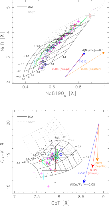
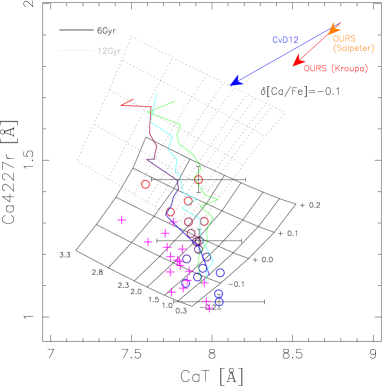
7.4 Unimodal vs. bimodal IMFs
Figs. 17 and 18 plot the results of fitting spectral indices with unimodal (i.e. single power law) IMF models. The corresponding IMF slope– trends are shown in Fig. 12 (middle panel), with the best-fitting coefficients of the – relation (Eq. 3) given in Tab. 3. As explained in Sec. 3, we have limited the range of unimodal slopes to . Indeed, the trends of with show that higher values of are not required to describe the data with single-slope IMFs.
Unimodal models provide a good fit to spectral indices, similar to bimodal IMFs. In particular, fits match well all selected spectral indices. At km s-1, the models give too high values of with respect to the observations, both for and models, as in the case with a bimodal IMF. The discrepancy disappears when including the effect of single element abundance ratios, with being more negative in lower mass galaxies. Indeed, the individual trends we find for , , and , vs. are very similar to the bimodal case, with small deviations from solar scale.
Unimodal models also feature a clear tendency for the IMF slope to increase with velocity dispersion, the best-fitting slope in Eq. 3 differing from zero at more than (see Tab. 4). However, the amount of variation is different from the bimodal case: ranges from to for a single-slope IMF, whereas best-fit bimodal IMF slopes vary from to . In fact, for models, the best-fitting slope of the – relation changes from for bimodal to for unimodal IMF. This difference arises from the fact that – at a given – unimodal and bimodal IMFs are characterized by a different fraction of high- to low-mass stars, and thus the has a different physical meaning for unimodal and bimodal models. Fig. 19 illustrates this point, where, instead of we use the mass fraction in stars with masses below some threshold, as a function of velocity dispersion. This mass fraction is given at “time zero”, by using the given functional form of the IMF over the stellar mass range from to M⊙ (as in Vazdekis et al. 1996). At a given , we use the value corresponding to the best-fit models to determine the mass fraction. Two cases are considered, corresponding to a threshold of and M⊙, respectively. The mass fractions agree pretty well between unimodal and bimodal IMFs. In particular, for M/M, the agreement is better than , proving that mass fractions are robustly constrained regardless of the adopted IMF shape. For M/M, the trends in the initial mass fraction for both unimodal and bimodal models can be described by the following relation:
| (4) |
where is the IMF. The coefficients are obtained by fitting simultaneously both trends, for stacks with km s-1(i.e. the range where a significant variation of with is detected, see Fig. 12). Eq. 4 is plotted in Fig. 19 as a dot-dashed curve. From Fig. 19 we conclude that the initial stellar mass fraction in low-mass stars (M/M) increases systematically in ETGs, from at km s-1 to at km s-1.
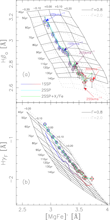
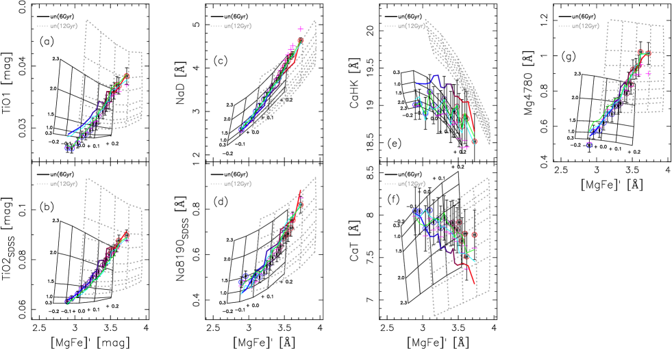
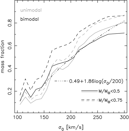
7.5 Hybrid approach
So far, the analysis is based on equivalent widths alone, to constrain both the IMF slope, , and the distribution of stellar ages and metallicities. As an additional test, we define a complementary probability distribution function based on spectral fitting, and we combine this information with our targeted IMF-sensitive line strengths, following a method analogous to the one described in FLD13. Furthermore, we consider here the effect of a more complex distribution of stellar ages and metallicities, by adopting a standard exponentially decaying star formation rate (i.e. a -model), where a star formation history is described by four parameters: formation epoch, exponential timescale, metallicity (kept fixed for each individual model), and IMF slope, where the bimodal function is chosen. Table 6 shows the range in parameters. For each stack, we explore a grid of models, defining two independent PDFs from the constraints on either spectral fitting or line strengths (we use in this analysis , , , , , , and ). We apply the same corrections for as in the rest of the paper. The final PDF is given by the product of the individual PDFs, enabling us to combine spectral fitting, to constrain the age and metallicity distribution, and individual line strengths, to target the IMF slope.
| Parameter | Steps | Range | Description |
|---|---|---|---|
| Formation Epoch | |||
| (Gyr) | Exponential timescale | ||
| Metallicity | |||
| IMF slope (bimodal) |
is the current () age of the Universe, i.e. 13.5 Gyr for a vanilla flavoured (; km s-1 Mpc-1) CDM cosmology.
The spectral fit is performed over the Å range 262626In contrast to Sec. 5.1, where we adopt an upper limit of Å, the value of Å is chosen here to avoid several features, like TiO molecular bands and , which are already taken into account as line strength constraints., after convolving the synthetic spectra, from the original Å resolution of the extended MILES (MIUSCAT) models, to a velocity dispersion of km s-1 (i.e. the maximum value of for stacked spectra), plus the SDSS spectral resolution. We avoid extending the fit over a wider range of wavelengths to minimise the effect of flux calibration systematics. Our results do not change significantly if a smaller spectral window is used, but it is important to include in the fitting range the region around the 4000 Å break for an effective constraint on the stellar ages. The bottom panel of Fig. 12 shows the best fit values of the IMF bimodal slope with respect to velocity dispersion, including error bars. In addition to the general model (black solid dots), we include, for reference, the constraints when only using the SED fit (red crosses), illustrating the expected complete degeneracy. The magenta open squares give the results when only using the targeted IMF-sensitive line strengths (i.e. , , , , and ). Finally, the full hybrid analysis is also shown for models comprising only simple stellar populations (i.e a single age and metallicity), as open grey dots. The figure confirms that our previous results are robust with respect to more complex distributions of stellar ages and metallicities. In particular, fitting Eq. 3 to the – trend, when only using the targeted IMF-sensitive line strengths (magenta dashed curve in the bottom panel of Fig. 12), we find consistent results to the fits of line strengths alone (see the values of best-fitting coefficients in Tab. 4). Also, the results of the hybrid approach can be compared to those of our previous work (FLD13), where we used the same hybrid approach to constrain the , but with a smaller set of spectral indices, no correction for abundance ratio at fixed , and we did not optimize the definition of TiO and Na indices. In FLD13, we reported a – slope of , consistent with that of found here (Tab. 4). On the other hand, the offset of the – relation reported by FLD13 (), is shallower than that of derived here from the hybrid approach, but fully consistent with that we derive from the analysis (, see Tab. 4).
Fig. 20 shows jointly and independently the constraining power of spectral fitting (SED) and line strength fitting (EWs). From top to bottom, the panels give the probability distribution function with respect to stellar age, metallicity, and IMF slope, for two different stacks, corresponding to a velocity dispersion of km s-1 (dashed line) and km s-1 (solid line). The figure shows that an analysis based exclusively on line strengths cannot discriminate between the different age distributions of galaxies with different velocity dispersion. Notice in the hybrid method we only use the IMF-sensitive indices, since the spectral fitting substitutes the age- and metallicity-sensitive indices: , and . In contrast, differences in IMF slope cannot be distinguished between these two stacks when using spectral fitting alone. It is the combination of the two that enables us to obtain strong constraints on , that are complementary to our previous analysis, only based on spectral lines. The hybrid method confirms the strong correlation between IMF slope and velocity dispersion, even when a complex distribution of ages and metallicities is allowed for. The middle panels reveal that only metallicities dex contribute to the analysis, in agreement with our previous results (see e.g. Fig. 10).

8 Expected colours and ratios
In addition to gravity-sensitive features from integrated light, the stellar IMF can affect indirectly other observable galaxy properties, like broad-band colours (see Goudfrooij & Kruijssen 2013) and mass-to-light ratios (hereafter ; see, e.g., Cappellari et al. 2012a; Ferré-Mateu et al. 2013). Hence, it is interesting to contrast the expectations from our best-fit stellar population models with those from broad-band photometry and (dynamical) estimates.
| Description | |
|---|---|
| – | SSP, unimodal IMF, , , Age Gyr |
| – | SSP, bimodal IMF, , , Age Gyr |
| observed, , km s-1 |
8.1 Variation of colours
Optical–NIR photometry provide additional constraints on the IMF, as a large fraction of M dwarfs can enhance the NIR light of a stellar population for an IMF heavier than Salpeter (see, e.g., Peletier et al. 1990), making optical–NIR colours significantly redder. In fact, an excess of reddening at optical–NIR wavelengths has been often invoked as an important argument against the steepening of the low mass end of the IMF with galaxy mass (see, e.g., Worthey, Ingermann & Serven 2011). In order to address this issue, we focus here on the bin at the highest velocity dispersion (i.e. km s-1), for which the extended MILES (MIUSCAT)-based fits give the most bottom-heavy IMF, i.e. and , for the unimodal and bimodal cases, respectively. Out of ETGs in this bin (see Tab. 1), galaxies have NIR (K-band) photometry available from the UKIDSS-LAS survey (see Paper I for details). The median for these galaxies 272727Notice that SDSS g-band photometry is in the AB system, while UKIDSS data are Vega-calibrated. As detailed in Paper I, colours are measured in an adaptive aperture of , where is the -band Kron radius. Median colours are corrected to the fibre aperture of radius , using colour gradient estimates from La Barbera et al. (2010c) (Paper IV). is reported in Tab. 7, and compared to the colour range of unimodal and bimodal extended MILES (MIUSCAT) models with bottom-heavy IMF. Model colours are estimated, for SSPs, using photometric stellar libraries, with the code of Vazdekis et al. (2010). To describe the high-mass systems, we consider only colours for metallicities equal or above solar, and old ages ( Gyr). The range of model colours in the Table is fully consistent with the observed , even for the reddest unimodal models. We remark here that a detailed comparison of constraints from spectral indices and broad-band colours is beyond the scope of the present paper and will be addressed in a forthcoming contribution. Notice also that although a varying IMF can affect significantly some optical colours (e.g. ), proper modelling of different optical colours for quiescent galaxies still represents a challenge for current stellar population models, and the effect of -enhancement on optical (as well as NIR) colours remains to be fully understood (see MIUSCAT-II). However, for the purpose of the present work, we emphasize that optical–NIR colours do not pose any problem for the hypothesis of a bottom-heavy IMF in massive ETGs.
8.2 Variation of M/L
Fig. 21 plots the median dynamical as a function of . The is estimated as (see, e.g., Cappellari et al. 2012b), where is the effective radius, is the central velocity dispersion corrected to an aperture of , is the gravitational constant, and is the total galaxy luminosity. Both and are measured for each galaxy by fitting seeing-convolved Sérsic models to the SDSS -band galaxy images (see SPIDER-I for details). The aperture correction to is performed by using eq. 1 of Cappellari et al. (2006). The above approximation for provides an estimate of the within with an accuracy of dex. This uncertainty is added in quadrature, for each bin, to the error on the median . We refer the reader to, e.g., Tortora et al. (2012); Cappellari et al. (2012b); Tortora et al. (2013) for a discussion on the impact of different model assumptions on the estimate of . For the purpose of the present work, we do not aim to discuss the details beyond the computation of , but instead, we focus on the comparison between the predictions of the stellar (hereafter ) from our best-fit population models with the estimates of the dynamical . The key aspect is the constraint that stellar mass-to-light ratios cannot exceed dynamical estimates, i.e. . The expected ’s are overplotted in Fig. 21, for , , and models, respectively, and for bimodal (upper-) and unimodal (lower-) models 282828 The estimates, as plotted in Fig. 21, are made available on request to the authors in tabular format, along with the same estimates obtained for a Kroupa Universal IMF. . The 1 confidence contours on are plotted only for models, for clarity. The Figure shows that a unimodal IMF gives too high, and thus unphysical, , with respect to the dynamical . Hence, although the unimodal models do fit spectral indices as well as the bimodal ones, they seem to be rejected based on the predictions. On the contrary, bimodal models give an broadly consistent with , even for strongly bottom-heavy models, as at highest . Considering error bars, our bimodal best-fits are also compatible with stellar mass-to-light ratios being smaller than the dynamical ones, leaving room for additional, non-stellar, matter (i.e. dark-matter). A similar conclusion has been recently drawn by Conroy & van Dokkum (2012b), for a subsample of ETGs from the SAURON survey. We remark that the above conclusions are based on the assumption that the expression for the dynamical from Cappellari et al. (2012b) applies to the whole population of ETGs, represented by our stacked spectra. Detailed dynamical and lensing studies for large samples of ETGs will help to address this point in the future.
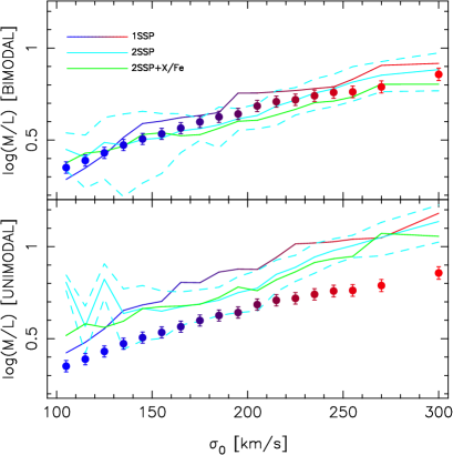
9 Summary
This paper explores in detail the recent claims of a systematic variation of the low-mass end of the IMF in massive early-type galaxies (ETGs). In order to set robust constraints, we need a large, representative dataset of galaxy spectra at very high signal-to-noise ratio. For this purpose, we stack a large, high-quality sample of SDSS spectra, comprising low redshift () ETGs from the SPIDER survey (La Barbera et al., 2010a). The stacking is performed in bins, corresponding to their central velocity dispersion, and, at fixed velocity dispersion, we also assemble a subsample split with respect to -enhancement, by using a solar-scale proxy (, see Fig. 6). We select a variety of IMF-sensitive spectral features (, , , , , see Fig. 4), along with additional indices strongly sensitive to the abundance of individual elements that could affect their interpretation. The analysis includes standard age and metallicity indicators (, , ). After being corrected to solar-scale by means of semi-empirical correlations among line strengths and at fixed , the indices are fitted with state-of-the-art population synthesis models. We use the extended MILES (MIUSCAT) library (Vazdekis et al., 2012), covering a wide range of age, metallicity, star-formation histories, and IMF. The analysis is complemented with an independent hybrid approach, where direct spectral fitting in the optical is combined with constraints from IMF-sensitive features (following our previous work, Ferreras et al., 2013). Two types of IMF are considered, a single power-law distribution, generalizing the Salpeter law, and a bimodal IMF, with a gradual turn-off at low mass, that generalizes the Kroupa case. The main results can be summarized as follows:
- i.
-
All selected spectral features consistently suggest a variation of IMF slope () in ETGs, with a trend from a Kroupa/Chabrier case at low central velocity dispersion, towards a more bottom-heavy IMF with increasing . For a bimodal IMF, the best-fit increases from about at km s-1 to almost at km s-1. For unimodal models, the slope varies from to over the same range (Fig. 12). The fits to the – correlation (eq. 3) give consistent values between different methods (Tab. 4), although we note that the physical quantity being constrained is the mass fraction in low-mass stars (see iii. below)
- ii.
-
Both unimodal and bimodal cases fit equally well all selected spectral indices, implying that we cannot distinguish between these two kinds of models based on the indices alone (see, e.g., Fig. 11 and 18). However, unimodal models seem to be clearly rejected by their overly high values of the stellar (relative to dynamical) mass-to-light () ratios (Fig. 21). On the other hand, the varying-IMF bimodal best-fits are in good agreement with independent constraints, i.e. dynamical estimates, and the optical-NIR broad-band colours of ETGs in our sample.
- iii.
-
Although unimodal and bimodal models cannot be distinguished with the present analysis, they predict very consistent stellar mass fractions at birth in low-mass stars ( M⊙), varying from at km s-1 to at km s-1(Fig. 19). Such stellar low-mass fractions (Eq. 4) represent the most robust constraint from the present analysis, and should be matched by theories aimed to explain the stellar IMF.
- iv.
-
The fact that both solar-scale corrected IMF- and abundance-sensitive line strengths from different species, i.e. Na, Ca, TiO, and Mg, can be all consistently explained by models with a varying IMF gives strong support to the claim that the IMF truly changes at the low-mass end in ETGs with high velocity dispersion, in constrast to a picture whereby single element adundances conspire to change simultaneously with . Indeed, including a varying abundance of Na, Ca, and Ti in our fits (based on Conroy & van Dokkum 2012a stellar population models), we find no evidence for a significant variation of these abundances with besides the general trend (Fig. 14).
- v.
-
The range of variation of IMF-sensitive line strengths with is essentially similar for both low- and high- stacks, implying that velocity dispersion (i.e. possibly galaxy mass) is the main driver of IMF variation, regardless of changes in -enhancement.
- vi.
-
Regarding the , we find a remarkably tight correlation between the (nearly) solar-scale proxy, , i.e. the difference between the two metallicities estimated from Mg and Fe lines with solar-scaled models, and the “true” , i.e. the one obtained by using -enhanced stellar population models (Fig 6). This proves that one can study abundance ratio effects by relying entirely on solar-scaled models.
- vii.
-
Besides and , we have also tried to fit the well-known Lick-based feature. This index remains a puzzle for current stellar population models, as no fitting scheme is able to match its line strengths, especially at high-, where model indices are far too high with respect to the observations (Fig. 16). The under-abundance explanation for this discrepancy seems to be excluded because the extended MILES (MIUSCAT) base models match well both the and features (see, e.g., Fig.11).
From the modelling point of view, the suggested change in the IMF of ETGs with velocity dispersion could be expected from the different physical properties of the star forming clouds during the formation of a massive galaxy (Larson, 2005) – such as a turbulent ISM with a very high Mach number (Hopkins, 2012). Alternatively, variations in the IMF properties convolved with the star formation history can leave its imprint on the so-called integrated galactic IMF (IGIMF, see, e.g., Kroupa & Weidner, 2003), which corresponds to the superposition of all populations ever formed, and constitutes the observable we really map with unresolved spectroscopic data. Regardless of whether the cause lies in the microphysics of star formation, or the global formation history, the robust constraints we impose here on the initial mass fraction in low-mass stars should be met by any theory of star formation.
Acknowledgments
We would like to thank the anonymous referee for his/her helpful report, which definitely helped improving parts of this manuscript. We also thank R. Smith for helpful comments on this manuscript. This paper is based on data retrieved from the Sloan Digital Sky Survey archives (http://www.sdss.org/collaboration/credits.html). We have also made use of the 4th data release of the UKIDSS survey (Lawrence et al., 2007), which is described in detail in Warren et al. (2007). Funding for the SDSS and SDSS-II has been provided by the Alfred P. Sloan Foundation, the Participating Institutions, the National Science Foundation, the U.S. Department of Energy, the National Aeronautics and Space Administration, the Japanese Monbukagakusho, the Max Planck Society, and the Higher Education Funding Council for England. JFB acknowledges support from the Ramón y Cajal programme by the Spanish Ministry of Economy and Competitiveness (MINECO). This work has been supported by the Programa Nacional de Astronomía y Astrofísica of MINECO, under grants AYA2010-21322-C03-01 and AYA2010-21322-C03-02 and by the Generalitat Valenciana under grant PROMETEO-2009-103.. MT acknowledges the support of FAPESP, process no. 2012/05142-5.
Appendix A Definition of and spectral indices
In the present work, we adopt a modified version of and NaI8200A spectral indices, previously defined by Trager et al. (1998) and Vazdekis et al. (2012), respectively. The NaI8200A index is, in turn, a modified version of the NaI doublet index proposed by Schiavon et al. (1997a). The reason for adopting a modified version of these indices is illustrated in Fig. 22, where we plot the stacked spectrum with km s-1 in the spectral range of ( Å; left) and NaI ( Å; right). Two extended MILES (MIUSCAT) SSP models, with age Gyr, solar metallicity (), and two different IMFs, i.e. (Kroupa-like) and , are overplotted. The SSPs have been smoothed to match the spectral resolution and velocity dispersion of the stack. The red hatched regions mark the central bandpasses of the indices, for which we keep the original definition of and NaI8200A. The grey hatched regions are the original sidebands of and NaI8200A. While there is good agreement between models and data in the blue (red) pseudo-continuum of (NaI8200A), for both IMFs, the models show a deviation from the observed spectrum in the red (blue) sidebands of (NaI8200A). The largest deviations are seen at Å and Å, and are also present in the other stacked spectra. The discrepancies are not removed by changing the age and metallicity (as well as IMF) of the SSP models, for Gyr and . Hence, we have re-defined the red (blue) sideband of (NaI8190A) in order to minimize any deviation between models and data. This is done as follows.
- 1.
-
We adopt the original definition of and NaI8190A, and compute the best-fit model to spectral indices (see Sec. 6). We assume here a Kroupa IMF in order to avoid any bias towards a -varying IMF (which is the hypothesis we want to test);
- 2.
-
For , we vary the position (i.e. the lowest wavelength endpoint, ) and width, , of the red sideband, minimizing the absolute deviation of the index equivalent width between models and data. To this effect, we keep the central band and blue sideband definitions fixed to those of . The absolute deviation is computed by summing up the EW absolute deviations for five stacks (, , , , and km s-1), spanning the whole velocity dispersion range. The deviation is minimized for Å and Å (see the green hatched region in the left panel of Fig. 22). We adopt this definition throughout the present work, referring to the corresponding spectral index as , to point out that the definition has been optimized for the SDSS spectra.
- 3.
-
For NaI8190A, we adopt a similar procedure to that at point 2 for , but varying the position of the blue sideband of the index. We impose the constraint Å, i.e. the value adopted in Vazdekis et al. (2012), in order to avoid overly reducing the region where the blue pseudo-continuum is measured. The minimum absolute deviation is obtained for Å, and Å (see the green hatched region in the right panel of the Figure). We refer to the corresponding spectral index as .
Repeating the entire procedure, but replacing and NaI8190A at step 1 with and gives very similar sideband definitions as those adopted here, proving that the procedure is self-consistent. We also experimented with changing the Kroupa IMF assumption in step 1 with a -varying bimodal IMF (blue-through-red curve in top panel of Fig. 12), finding the optimum definitions of and to change by only a few Angström.
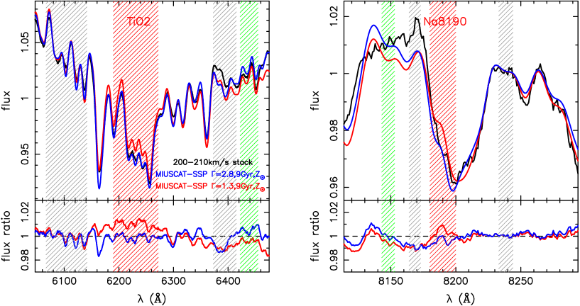
In Fig. 23, we show the dependence of and EWs on velocity dispersion. These indices have the further advantage to be less sensitive to resolution than the previously defined and NaI8200A. For , the decreased sensitivity is due to the fact that the blue sideband is measured in a more distant region from the feature. We also note that, as shown in Sec. 4, the new and indices have similar sensitivity to age, metallicity, and IMF as and NaI8200A.

Appendix B Emission correction to
In order to fit the spectral indices with stellar population models, we correct the spectral index for contamination from nebular emission. The presence of such contamination in our stacked spectra of ETGs is shown in Fig. 24, where we plot the spectral region around the [OII] feature at Å for the stacks at the endpoints of the velocity dispersion range, i.e. km s-1 (top) and km s-1 (bottom), respectively. Best-fitting extended MILES (MIUSCAT) models, obtained by direct fitting of the spectral region of interest are overplotted in grey (assuming a Kroupa IMF). Notice the flux excess at Å, in particular at the lowest , revealing the presence of nebular emission in the spectra.
The correction procedure to is illustrated in Fig. 25. For a given IMF (either bimodal or unimodal), we fit the spectral region (from to Å) with a linear combination of two MIUSCAT SSPs, excluding the trough of the line (i.e. from to Å). To improve the matching of the continuum, a multiplicative fourth degree polynomial is also used in the fitting. The residuals (bottom panel of the Figure) are fitted with a Gaussian function. The emission correction is given by the difference between the index of the stack and the one re-measured on the same stack after adding the Gaussian fit. By definition, this procedure will depend on the assumed IMF. For instance, for the km s-1 ( km s-1) stack, the emission correction varies from Å ( Å) for , to Å ( Å) for (bimodal IMFs). Although the dependence is small, following our previous work (FLD13), we have implemented an iterative procedure for the and models (see Sec. 6). First, we correct with the median correction (among all IMFs), and then we fit the spectral indices. Once the best-fit is derived, the emission correction is updated accordingly, and the fitting is repeated again. In practice, we found that further iterations are not required, as the fits do not change appreciably when performing a second iteration. Notice that in FLD13 we applied a similar procedure to that described here. However, rather than fitting the stacks with two MIUSCAT SSPs in the spectral region, we ran the STARLIGHT spectral fitting code over a larger spectral range. We found that the two SSP fits provide more robust results than our previous approach, being less sensitive to the adopted IMF. We note that either varying the degree of the multiplicative polynomial between two and six, or changing the size of the line trough, excluded from the fitting, between and Å, does not produce any significant change to our results. The correction turns out to vary smoothly with , from at lowest to for km s-1, further confirming the robustness of our approach.
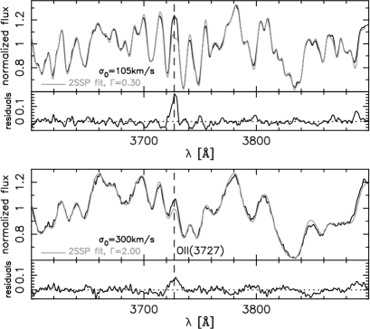
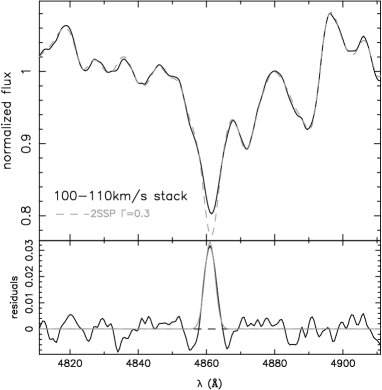
Appendix C Aperture effects
Given that the spectra used in this paper correspond to the central 3 arcsec region of each galaxy, a significant radial gradient of the properties of the stellar populations could affect the results. In Fig. 26 we explore this issue by showing, in the rightmost panels the variation of three of the most IMF-sensitive line strengths, with respect to effective radius, in comparison to the SDSS 3 arcsec diameter fibre. The shaded regions encompass the confidence level of the km s-1 (black) and km s-1 (grey) stacks. For reference, the panels on the left show the variation of the line strengths over the whole range in velocity dispersion. The figure confirms that our results are not affected by variations in radial gradients of the stellar populations.
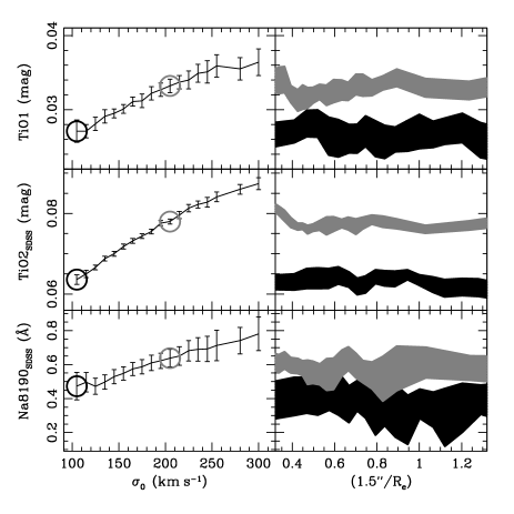
Appendix D Synthetic SSPs with varying abundance ratios
In addition to the CvD12 stellar population models, we have also tested the effect of individual variations of Ca, Na, and Ti abundances on the targeted spectral indices by creating a set of simplified SSP models. Empirical stellar libraries are not well suited for this purpose, since they are restricted to abundance patterns of stars in the solar neighbourhood. For this reason, we rely completely on synthetic stellar libraries. To generate stellar spectra, we use the Padova evolutionary tracks (Bertelli et al., 2008), identifying 16 – pairs along the Gyr isochrone, from the tip of the RGB ( K and ) down to the main sequence locus corresponding to a stellar mass of 0.15 M⊙ ( K and ). For each – pair. we generate synthetic stellar spectra with the PFANT code described in Cayrel et al. (1991), Barbuy et al. (2003) and Coelho et al. (2005). Given a stellar model atmosphere and lists of atomic and molecular lines, the code computes a synthetic spectrum assuming local thermodynamic equilibrium (LTE). We have used a refined atomic and molecular line list, calibrated through several stellar spectroscopic studies (see, e.g., Barbuy et al., 2003). For stellar atmosphere models, we used the MARCS 1D hydrostatic LTE models (Gustafsson et al., 2008). For , the atmospheric model geometry is plane-parallel and mass independent; for (giants with non-negligible photospheric depths), the models are calculated for a spherical geometry. In the latter case, models for 1 M⊙ are adopted. A microturbulent velocity of km s-1 is adopted for all spectra. Notice that the flux predictions of PFANT are less accurate in the blue part of the spectrum, in particular at Å, because of the so-called “predicted lines” problem (Kurucz, 1992). For this reason, the use of our synthetic SSPs to model features at wavelengths bluer than 5000 (e.g., the , see Sec. 7.3) should be taken with some caution.
The SSP spectra, corresponding to an age of 12 Gyr, are created using the integral
where is the spectrum of an individual star with mass at a given , and is the (assumed) IMF. We adopt a mass interval from M⊙ to M⊙. We consider Kroupa as well as unimodal IMFs, the latter with , (i.e. Salpeter) and , respectively. Notice that stars with M M⊙ are not included in the synthesis, as there are no Padova evolutionary tracks available below this mass limit. As discussed by CvD12, even in the case of a strongly bottom-heavy population (e.g. ), this approximation should have little impact on the results, because of the negligible contribution of stars with 0.08 M⊙ to the SSP integrated light. Fig. 27 compares one of our simple SSPs, with solar composition, to a MILES extended (MIUSCAT) SSP, with similar age, metallicity, and the same (Kroupa) IMF. Despite of the simple approach to create the synthetic models, the agreement with the MILES extended models is fairly good, with an rms of at Å, and in the bluer part of the spectrum ( Å). We remind the reader that the simplified SSPs presented here are used only in a relative sense, i.e. to compute differences in the spectral indices when varying individual element abundances. We also notice that our synthetic SSPs are based on rather different ingredients than the CvD12 ones. In particular, we use the MARCS and PFANT codes for the atmospheric models and stellar spectra, while CvD12 adopt the ATLAS12 (Kurucz, 1970) and SYNTHE (Kurucz & Avrett, 1981) codes, respectively. CvD12 adopt atomic and molecular line lists with oscillator strengths computed either theoretically or from lab measurements, while our oscillator strengths have been calibrated through several stellar spectroscopic studies. The synthetic stellar spectra in both models are created down to a stellar mass of 0.15 . However, CvD12 extrapolate the library down to 0.08 , while we completely disregard these low-mass stars. Finally, we use Padova evolutionary tracks, while CvD12 use Dartmouth isochrones (Dotter et al., 2008).
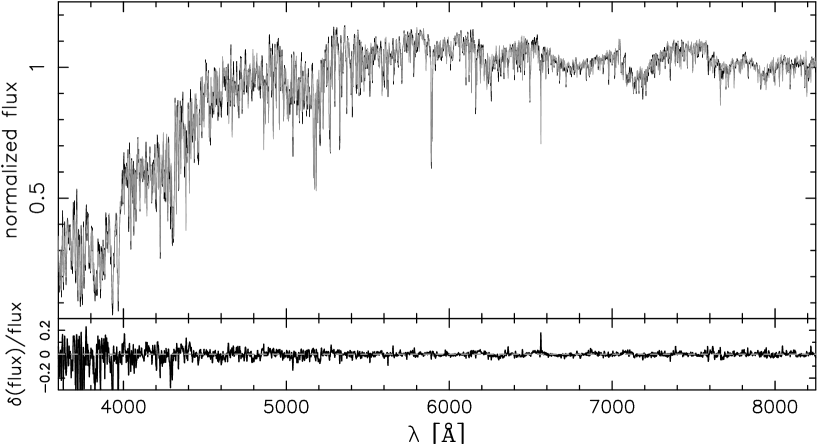
References
- Abazajian et al. (2009) Abazajian, K. N., et al., 2009, ApJS, 182, 543
- Adelman-McCarthy et al. (2008) Adelman-McCarthy, J.K., Agüeros, M.A., Allam, S.S., et al., 2008, ApJS, 175, 297
- Auger et al. (2010) Auger, M.W., Treu, T., Bolton, A.S., Gavazzi, R., Koopmans, L.V.E., Marshall, P.J., Moustakas, L.A., Burles, S., 2010, ApJ, 724, 511
- Barbuy et al. (2003) Barbuy B., Perrin M.-N., Katz D., Coelho P., Cayrel R., Spite M., Van’t Veer-Menneret C., 2003, A&A, 404, 661
- Barnabé et al. (2011) Barnabé, M., Czoske, O., Koopmans, L.V.E., Treu, T., Bolton, A.S., 2011, MNRAS, 415, 2215
- Bastian et al (2006) Bastian, N., Saglia, R.P., Goudfrooij, P., Kissler-Patig, M., Maraston, C., Schweizer, F., Zoccali, M., 2006, A&A, 448, 881
- Bastian et al. (2010) Bastian, N., Covey, K. R. & Meyer, M. R. 2010, ARA&A, 48, 339
- Bernardi et al. (2003a) Bernardi, M., et al., 2003a, AJ, 125, 1817
- Bernardi et al. (2003b) Bernardi, M., Sheth, R.K., Annis, J. 2003b, AJ, 125, 1849
- Bernardi et al. (2005) Bernardi, M., Sheth, R. K., Nichol, R. C., Schneider, D. P. & Brinkmann, J. 2005, AJ, 129, 61
- Bertelli et al. (2008) Bertelli, G. et al. 2008, A&A, 484, 815
- Bruzual & Charlot (2003) Bruzual, G., & Charlot, S. 2003, MNRAS, 344, 1000 (BC03)
- Cappellari et al. (2006) Cappellari, M., et al., 2006, MNRAS, 366, 1126
- Cappellari et al. (2012a) Cappellari, M., et al., 2012, Nature, 484, 485
- Cappellari et al. (2012b) Cappellari, M., et al., 2012, MNRAS, submitted (arXiv:1208.3522)
- Cappellari et al. (2012c) Cappellari, M., et al., 2012c, MNRAS, submitted (arXiv:1208.3523)
- Cardelli, Clayton & Mathis (1989) Cardelli, J. A., Clayton, G. C., Mathis, J. S., 1989, ApJ, 345, 245
- Carter et al. (1986) Carter, D., Visvanathan, N., Pickles, A.J., 1986, ApJ, 311, 637
- Cayrel et al. (1991) Cayrel, R., Perrin, M.-N., Barbuy, B., Buser, R., 1991, A&A, 247, 108
- Chabrier (2003) Chabrier, G., PASP, 115, 763
- Cid Fernandes et al. (2005) Cid Fernandes, R., Mateus, A., Sodré, L., Stasinska, G., Gomes, J. M., 2005, MNRAS, 358, 363
- Capaccioli, Caon & D’Onofrio (1992) Capaccioli, M., Caon, N., & D’Onofrio, M. 1992, MNRAS, 259, 323
- Cenarro et al. (2001) Cenarro, A. J., Cardiel, N., Gorgas, J., Peletier, R. F., Vazdekis, A., Prada, F., 2001, MNRAS, 326, 959
- Cenarro et al. (2003) Cenarro, A. J., Gorgas, J., Vazdekis, A., Cardiel, N., Peletier, R. F., 2003, MNRAS, 339, L12
- Cervantes et al. (2007) Cervantes, J. L., Coelho, P., Barbuy, B., and Vazdekis, A., 2007, Proceedings IAU Symposium No. 241 ’Stellar Populations as Building Blocks of Galaxies’, A. Vazdekis and R.F. Peletier, eds, 167
- Cervantes & Vazdekis (2009) Cervantes, J. L., Vazdekis, A., 2009, MNRAS, 392, 691
- Coelho et al. (2005) Coelho, P., Barbuy, B., Meléndez, J., Schiavon, R. P., Castilho, B. V., 2005, A&A, 443, 735
- Coelho et al. (2007) Coelho, P., Bruzual, G., Charlot, S., Weiss, A., Barbuy, B., Ferguson, J.W., 2007, MNRAS, 382, 498
- Cohen (1978) Cohen, J. G., 1978, ApJ, 221, 788
- Conroy & van Dokkum (2012a) Conroy, C., van Dokkum, P., 2012a, ApJ, 747, 69
- Conroy & van Dokkum (2012b) Conroy, C., van Dokkum, P., 2012b, ApJ, 760, 71
- de la Rosa et al. (2012) de la Rosa, I. G., la Barbera, F., Ferreras, I., de Carvalho, R. R. 2012, MNRAS, 418, L74
- Delisle & Hardy (1992) Delisle, S., Hardy, E., 1992, AJ, 103, 711
- Diaz, Terlevich, Terlevich (1989) Diaz, A.I., Terlevich, E., Terlevich, R., 1989, MNRAS, 239, 325
- Dotter et al. (2008) Dotter, A., Chaboyer, B., Jevremović, D., Kostov, V., Baron, E., Ferguson, J. W., 2008, ApJ, 178, 89
- Dutton, Mendel & Simard (2012) Dutton, A. A., Mendel, J. T., Simard, L., 2012, MNRAS, 422, 33
- Faber & French (1980) Faber, S.M., French, H.B., 1980, ApJ, 235, 405
- Falcón-Barroso et al. (2011) Falcón-Barroso, J., Sánchez-Blázquez, P., Vazdekis, A., Ricciardelli, E., Cardiel, N., Cenarro, A. J., Gorgas, J., Peletier, R. F., 2011, A&A, 532, 95
- Ferreras et al. (2005) Ferreras, I., Saha, P., Williams, L. L. R., 2005, ApJ, 623, 5
- Ferreras et al. (2008) Ferreras, I., Saha, P., Burles, S., 2008, MNRAS, 383, 857
- Ferreras et al. (2010) Ferreras, I., Saha, P., Leier, D., Courbin, F., Falco, E. E. 2010, MNRAS, 409, L30
- Ferreras et al. (2013) Ferreras, I., La Barbera, F., de la Rosa, I. G., Vazdekis, A., de Carvalho, R. R., Falcón-Barroso, J., Ricciardelli, E., 2013, MNRAS, 429, L15 (FLD13)
- Ferré-Mateu et al. (2013) Ferré-Mateu, A., Vazdekis, A., de la Rosa, I. G., 2013, MNRAS, in press (arXiv:1301.7066)
- Gallazzi et al. (2006) Gallazzi, A., et al. 2006, MNRAS, 370, 1106
- González (1993) González, J. J. 1993, Ph.D. thesis, Univ. California
- Goudfrooij & Kruijssen (2013) Goudfrooij, P., Kruijssen, J.M.D., 2013, ApJ, 762, 107
- Graham & Guzmán (2003) Graham, A. W., Guzmán, R., 2003, AJ, 125, 2936
- Gustafsson et al. (2008) Gustafsson, B., Edvardsson, B., Eriksson, K., Jørgensen, U. G., Nordlund, Å., 2008, A&A, 486, 951
- Hardy & Couture (1988) Hardy, E., Couture, J., 1988, ApJ, 325, 29
- Hopkins (2012) Hopkins, P., 2013, arXiv:1204.2835
- Johansson et al. (2012) Johansson, J., Thomas, D., Maraston, C., 2012, MNRAS, 421, 1908
- Kroupa (2001) Kroupa, P., 2001, MNRAS, 322, 231
- Kroupa & Weidner (2003) Kroupa, P., Weidner, C. 2003, ApJ, 598, 1076
- Kurucz (1970) Kurucz, R. L., 1970, SAOR, 309
- Kurucz & Avrett (1981) Kurucz, R. L., Avrett, E. H., 1981, SAOR, 391
- Kurucz (1992) Kurucz, R.L., 1992, RMxAA, 23, 45
- La Barbera et al. (2010a) La Barbera, F., de Carvalho, R. R., de la Rosa, I.G., Lopes, P.A.A., Kohl-Moreira, J.L., Capelato, H.V., 2010a, MNRAS, 408, 1313 (Paper I)
- La Barbera et al. (2010b) La Barbera, F., de Carvalho, R.R., de la Rosa, I.G., Lopes, P.A.A., 2010, MNRAS, 408, 1335 (Paper II)
- La Barbera et al. (2010c) La Barbera, F., de Carvalho, R. R., de la Rosa, I.G., Gal, R. R., Swindle, R., Lopes, P.A.A., 2010c, AJ, 140, 1528 (Paper IV)
- Larson (2005) Larson, R. B., 2005, MNRAS, 359, 211
- Lawrence et al. (2007) Lawrence, A., Warren, S.J., Almaini, O., et al. 2007, MNRAS, 379, 1599
- Peletier et al. (1990) Peletier, R.F. et al. 1990, A&A, 233, 62
- Prochaska, Rose & Schiavon (2005) Prochaska, L. C., Rose, J. A., Schiavon, R. P., 2005, AJ, 130, 2666
- Ricciardelli et al. (2012) Ricciardelli, E., Vazdekis, A., Cenarro, A. J., Falcón-Barroso, J., 2012, MNRAS, 424, 172 (MIUSCAT-II)
- Rogers et al. (2010) Rogers B., Ferreras I., Peletier, R., Silk, J., 2010, MNRAS, 402, 447
- Salpeter (1955) Salpeter, E. E. 1955, ApJ, 121, 161
- Sánchez-Blázquez et al. (2006) Sánchez-Blázquez, P. et al. 2006, MNRAS, 371, 703
- Schiavon et al. (1997a) Schiavon, R., Barbuy, B., Rossi, S. C. F., Milone, A., 1997, ApJ, 479, 902
- Schiavon et al. (1997b) Schiavon, R., Barbuy, B., Rossi, S. C. F., Milone, A., 1997, ApJ, 479, 902
- Schiavon et al. (2002) Schiavon, R.P., Faber, S.M., Rose, J. A., Castilho, B. V., 2002, ApJ, 580, 873
- Schiavon, Caldwell & Rose (2004) Schiavon, R., Caldwell, N., Rose, J. A., 2004, AJ, 127, 1513
- Serven et al. (2005) Serven, J., Worthey, G., Briley, M. M., 2005, ApJ, 627, 754
- Serven & Worthey (2007) Serven, J., Worthey, G., 2010, AJ, 140, 152
- Serra & Trager (2007) Serra, P., Trager, S. C., 2007, MNRAS, 374, 769
- Smith, Lucey & Carter (2012) Smith, R. J., Lucey, J. R., Carter, D., 2012, MNRAS, 426, 2994
- Spiniello et al. (2012) Spiniello, C., Trager, S. C., Koopmans, L. V. E., Chen, Y. P., 2012, ApJ, 753, 32
- Spinrad (1962) Spinrad, H., 1962, ApJ, 135, 715
- Swindle et al. (2011) Swindle, R., Gal, R. R., La Barbera, F., de Carvalho, R. R., 2011, AJ, 142, 118S (Paper V)
- Thomas et al. (2003a) Thomas D., Maraston C., Bender R., 2003, MNRAS, 339, 897
- Thomas et al. (2003b) Thomas D., Maraston C., Bender R., 2003, MNRAS, 343, 279
- Thomas et al. (2004) Thomas D., Maraston C., Korn A., 2004, MNRAS, 351, L19
- Thomas et al. (2005) Thomas, D., et al. 2005, ApJ, 621, 673
- Thomas & Davies (2006) Thomas D., Davies R.L., 2006, MNRAS, 366, 510
- Thomas, Johansson & Maraston (2011) Thomas, D., Johansson, J., Maraston, C., 2011, MNRAS, 412, 2199
- Thomas, Maraston & Johansson (2011) Thomas, D., Maraston, C., Johansson, J., 2011, MNRAS, 412, 2183
- Thomas et al. (2011) Thomas, J., et al., 2011, MNRAS, 415, 545
- Trager et al. (1998) Trager, S. C., Worthey, G., Faber, S. M., Burstein, D., González, J. J., 1998, ApJS, 116, 1
- Tortora et al. (2012) Tortora, C., La Barbera, F., Napolitano, N. R., de Carvalho, R. R., Romanowsky, A. J., 2012, MNRAS, 425, 577 (Spider V)
- Tortora et al. (2013) Tortora, C., Romanowsky, A.J., Napolitano, N., 2013, ApJ, in press ()
- Trager et al. (2000) Trager, S. C., Faber, S. M., Worthey, G., González, J. J. 2000, AJ, 120, 165
- Treu et al. (2010) Treu, T., Auger, M.W., Koopmans, L.V.E., Gavazzi, R., Marshall, P.J., Bolton, A.S., 2010, ApJ, 709, 1195
- Trevisan et al. (2012) Trevisan, M., Ferreras, I., de la Rosa, I. G., La Barbera, F., de Carvalho, R. R. 2012, ApJ, 752, L27
- van Dokkum & Conroy (2010) van Dokkum, P.G., Conroy, C., 2010, Nature, 468, 940
- van Dokkum & Conroy (2011) van Dokkum, P.G., Conroy, C., 2011, ApJ, 735, 13
- Vazdekis et al. (1996) Vazdekis, A., Casuso, E., Peletier, R.F., Beckman, J.E., 1996, ApJS, 106, 307
- Vazdekis et al. (1997) Vazdekis, A., Peletier, R.F., Beckman, J.E., Casuso, E., 1997, ApJS, 111, 203
- Vazdekis et al. (2001) Vazdekis, A., Salaris, M., Arimoto, N., Rose, J.A., 2001, ApJ, 549, 274
- Vazdekis et al. (2003) Vazdekis, A., Cenarro, A.J., Gorgas, J., Cardiel, N., Peletier, R.F., 2003, MNRAS, 340, 1317
- Vazdekis et al. (2010) Vazdekis, A., Sánchez-Blázquez, P., Falcón-Barroso, J., et al. 2010, MNRAS, 404, 1639
- Vazdekis et al. (2012) Vazdekis, A., Ricciardelli, E., Cenarro, A.J., Rivero-González, J.G., Díaz-Garcá, L.A., Falcón-Barroso, J., 2012, MNRAS, 424, 157 (MIUSCAT-I)
- Yamada et al. (2006) Yamada, Y., Arimoto, N., Vazdekis, A., Peletier, R.F., 2006, ApJ, 637, 200
- Warren et al. (2007) Warren, S. J., Hambly, N. C., Dye, S., et al. 2007, MNRAS, 375, 213
- Wegner et al. (2012) Wegner, G.A., Corsini, E.M., Thomas, J., Saglia, R.P., Bender, R., Pu, S.B., 2012, MNRAS, 144, 78
- Wing & Ford (1969) Wing, R.F., Ford, Jr., W.K., 1969, PASP, 81, 527
- Worthey, Ingermann & Serven (2011) Worthey, G., Ingermann, B.A., Serven, J., 2011, ApJ, 729, 148
- Worthey (1998) Worthey, G., 1998, PASP, 110, 888