Exponents of interchain correlation for self-avoiding walks and knotted self-avoiding polygons

Erica Uehara and Tetsuo Deguchi Department of Physics, Graduate School of Humanities and Sciences, Ochanomizu University, 2-1-1 Ohtsuka, Bunkyo-ku, Tokyo 112-8610, Japan deguchi@phys.ocha.ac.jp
Abstract

We show numerically that critical exponents for two-point interchain correlation of an infinite chain characterize those of finite chains in Self-Avoiding Walk (SAW) and Self-Avoiding Polygon (SAP) under a topological constraint. We evaluate short-distance exponents θ​(i,j)πœƒπ‘–π‘—\theta(i,j) through the probability distribution functions of the distance between the i𝑖ith and j𝑗jth vertices of N𝑁N-step SAW (or SAP with a knot) for all pairs (1≀i,j≀Nformulae-sequence1𝑖𝑗𝑁1\leq i,j\leq N). We construct the contour plot of θ​(i,j)πœƒπ‘–π‘—\theta(i,j), and express it as a function of i𝑖i and j𝑗j. We suggest that it has quite a simple structure. Here exponents θ​(i,j)πœƒπ‘–π‘—\theta(i,j) generalize des Cloizeaux’s three critical exponents for short-distance interchain correlation of SAW, and we show the crossover among them. We also evaluate the diffusion coefficient of knotted SAP for a few knot types, which can be calculated with the probability distribution functions of the distance between two nodes.

1 Introduction

Polymers with nontrivial topology such as cyclic polymers have attracted much interest in several fields. Ring polymers are observed in nature such as circular DNA whose topology is given by the trivial knot (Fig. 1), while DNA with nontrivial knots are derived in experiments [1, 2, 3]. Naturally occurring proteins whose ends connected to give a circular topology has been recently discovered [4]. Due to novel developments in experimental techniques, ring polymers are now effectively synthesized in chemistry [5, 6, 7, 8, 9]. Moreover, polymers of topologically complex structures, which are sometimes called topological polymers, have been synthesized and separated with respect to their hydrodynamic radii such as through GPC [10, 11]. It is thus an interesting theoretical problem to calculate physical quantities such as the hydrodynamic radius, i.e. the diffusion coefficient, of each topological type. It can be derived through interchain correlation of the polymer chain by Kirkwood’s approximation. Here we remark that the topology of a ring polymer is specified by a knot, and it gives the simplest and most fundamental example of nontrivial topologies.

Topological constraints often play a central role in the statistical and dynamical properties of ring polymers in solution [12, 13, 14]. For instance, the mean-square radius of gyration of ring polymers under a topological constraint can be much larger than that of no topological constraint, in particular, at the ΞΈπœƒ\theta temperature of the corresponding linear polymers [15, 16, 17, 18, 19, 20, 21]. We call the phenomenon topological swelling. It is also confirmed in an experiment [22]. Due to the strong finite-size effect, however, it is not easy to determine numerically the exponent of the mean square radius of gyration for knotted ring polymers in ΞΈπœƒ\theta solution [20]. It is thus interesting to study topological effects on the scaling behavior of two-point correlations for Self-Avoiding Polygons or random polygons through simulation.

The Self-Avoiding Walk (SAW) and the Self-Avoiding Polygon (SAP) are fundamental theoretical models for linear and ring polymers in good solution, respectively [23, 24]. The scaling behavior of SAW is studied through the Monte-Carlo simulation and the renormalization group approach [25]. Correlations among configurations of SAW and SAP are nontrivial due to the excluded volume effect, and have attracted much interest in theoretical studies [26, 27, 28, 29, 30, 31, 32, 33, 34, 35, 36, 37]. SAP has several different points from SAW: It is not only that SAP has cyclic symmetry while SAW has two ends and no translational symmetry, but also that SAP has a topological constraint specified by a knot. However, we shall show that several short-chain scaling properties of SAW are useful for describing those of SAP.

Refer to caption
Figure 1: Trivial knot, 01subscript010_{1} (left), and the trefoil knot, 31subscript313_{1} (right).

In this paper, we study the scaling behavior of interchain correlation for SAW and off-lattice SAP with a fixed knot type through the Monte-Carlo simulation. In particular, we evaluate exponents for short-distance correlation for any pair of segments in a SAW or SAP under a topological constarint. We numerically determine the probability distribution function of the distance between two vertices i𝑖i and j𝑗j of the chain, from which we evaluate the exponent θ​(i,j)πœƒπ‘–π‘—\theta(i,j) for short-distance correlation and the exponent δ𝛿\delta for long-distance asymptotic behavior. The estimates of exponents θ​(i,j)πœƒπ‘–π‘—\theta(i,j) and δ𝛿\delta are useful for expressing physical quantities such as the diffusion coefficient and the structure factor of SAW or SAP as an approximate integral form. For SAW, exponents θ​(i,j)πœƒπ‘–π‘—\theta(i,j) generalize des Cloizeaux’s three exponents ΞΈssubscriptπœƒπ‘ \theta_{s} (s=0,1,2)s=0,1,2) for short-distance interchain correlation of an infinite chain, which we shall define shortly. We shall show that the estimates of exponents θ​(i,j)πœƒπ‘–π‘—\theta(i,j) corresponding to ΞΈssubscriptπœƒπ‘ \theta_{s} (s=0,1,2)s=0,1,2) are roughly similar to or a little smaller than the theoretical values of ΞΈssubscriptπœƒπ‘ \theta_{s}. The difference may be due to the finiteness of the chain investigated. We also show the crossover among them. For SAP consisting of cylindrical segments we show that exponents θ​(i,j)πœƒπ‘–π‘—\theta(i,j) and δ𝛿\delta of SAP with large excluded volume are close to those of SAW, while exponents θ​(i,j)πœƒπ‘–π‘—\theta(i,j) and δ𝛿\delta for SAP with small excluded volume are much smaller than those of SAW and close to those of Random Walks.

Let us briefly review the scaling behavior of interchain correlation of SAW. We denote by p0​(𝒓;N)subscript𝑝0𝒓𝑁p_{0}({\mbox{\boldmath$r$}};N) the probability distribution function of the end-to-end vector 𝒓𝒓r of an N𝑁N-step SAW. Considering the rotational symmetry we express it also as p0​(r;N)subscript𝑝0π‘Ÿπ‘p_{0}(r;N) where rπ‘Ÿr is the end-to-end distance: r=|𝒓|π‘Ÿπ’“r=|{\mbox{\boldmath$r$}}|. The large-rπ‘Ÿr asymptotic behavior of p0​(r;N)subscript𝑝0π‘Ÿπ‘p_{0}(r;N) was argued [26] as

p0​(r;N)∼RNβˆ’d​A​(r/RN)​exp⁑(βˆ’(r/RN)Ξ΄)similar-tosubscript𝑝0π‘Ÿπ‘superscriptsubscriptπ‘…π‘π‘‘π΄π‘Ÿsubscript𝑅𝑁superscriptπ‘Ÿsubscript𝑅𝑁𝛿p_{0}(r;N)\sim R_{N}^{-d}A(r/R_{N})\exp\left(-(r/R_{N})^{\delta}\right) (1)

where RN=R0​NΞ½subscript𝑅𝑁subscript𝑅0superscriptπ‘πœˆR_{N}=R_{0}N^{\nu} and Ξ΄=1/(1βˆ’Ξ½)𝛿11𝜈\delta=1/(1-\nu). Here the scaling exponent ν𝜈\nu is given by Ξ½β‰ˆ0.588𝜈0.588\nu\approx 0.588. The small-rπ‘Ÿr behavior of p0​(r;N)subscript𝑝0π‘Ÿπ‘p_{0}(r;N) was studied analytically [27]. By assuming a scaling function F0​(y)subscript𝐹0𝑦F_{0}(y) satisfying p0​(r;N)=RNβˆ’d​F0​(r/RN)subscript𝑝0π‘Ÿπ‘superscriptsubscript𝑅𝑁𝑑subscript𝐹0π‘Ÿsubscript𝑅𝑁p_{0}(r;N)=R_{N}^{-d}F_{0}(r/R_{N}), it was shown that the short distance behavior is given by

F0​(y)∼yga​syβ†’0.formulae-sequencesimilar-tosubscript𝐹0𝑦superscript𝑦𝑔a𝑠→𝑦0F_{0}(y)\sim y^{g}\quad{\mbox{a}s}\quad y\rightarrow 0\,. (2)

with g=(Ξ³+1βˆ’dβ€‹Ξ½βˆ’Ξ±)/ν𝑔𝛾1π‘‘πœˆπ›Όπœˆg=(\gamma+1-d\nu-\alpha)/\nu. The exponent g𝑔g was also derived through renormalization group (RG) arguments [28]. Here we have g=(Ξ³βˆ’1)/ν𝑔𝛾1𝜈g=(\gamma-1)/\nu through the scaling relation: Ξ±=2βˆ’d​ν𝛼2π‘‘πœˆ\alpha=2-d\nu. It is also derived via RG arguments with the blob picture [23].

Short-distance correlation between two points of a long polymer in a good solvent was studied by des Cloizeaux with the RG techniques [29]. The exponents of the short-distance correlation, ΞΈssubscriptπœƒπ‘ \theta_{s} for s=0,1,2𝑠012s=0,1,2, were defined through the probability distribution functions ps​(r,N)subscriptπ‘π‘ π‘Ÿπ‘p_{s}(r,N) of the distance between two given vertices of an N𝑁N-step SAW in the large-N𝑁N limit as follows. We denote by p1​(r,N)subscript𝑝1π‘Ÿπ‘p_{1}(r,N) the probability distribution function of the distance between an end point and a middle point of the SAW, and by p2​(r,N)subscript𝑝2π‘Ÿπ‘p_{2}(r,N) that of the distance between two points in the middle region of the SAW. Assuming that ps​(r,N)β‰ˆRNβˆ’d​Fs​(r/RN)subscriptπ‘π‘ π‘Ÿπ‘superscriptsubscript𝑅𝑁𝑑subscriptπΉπ‘ π‘Ÿsubscript𝑅𝑁p_{s}(r,N)\approx R_{N}^{-d}F_{s}(r/R_{N}), we define the critical exponents ΞΈssubscriptπœƒπ‘ \theta_{s} for short distance correlation by

Fs​(y)∼yΞΈsa​syβ†’0,fors=0,1,2.formulae-sequencesimilar-tosubscript𝐹𝑠𝑦superscript𝑦subscriptπœƒπ‘ a𝑠formulae-sequence→𝑦0for𝑠012F_{s}(y)\sim y^{\theta_{s}}\quad{\mbox{a}s}\quad y\rightarrow 0\,,\quad\mbox{for}\quad s=0,1,2. (3)

Here we remark that exponent g𝑔g in eq. (2) corresponds to ΞΈ0subscriptπœƒ0\theta_{0}. The exponents ΞΈssubscriptπœƒπ‘ \theta_{s} for s=0,1,2𝑠012s=0,1,2 were calculated by des Cloizeaux with RG techniques in terms of the Ο΅italic-Ο΅\epsilon-expansion upto the second order [29]. The estimates for d=3𝑑3d=3 are given by

ΞΈ0(R​G)=0.273,ΞΈ1(R​G)=0.46,ΞΈ2(R​G)=0.71.formulae-sequencesuperscriptsubscriptπœƒ0𝑅𝐺0.273formulae-sequencesuperscriptsubscriptπœƒ1𝑅𝐺0.46superscriptsubscriptπœƒ2𝑅𝐺0.71\theta_{0}^{(RG)}=0.273,\quad\theta_{1}^{(RG)}=0.46,\quad\theta_{2}^{(RG)}=0.71. (4)

In the RG derivation of ΞΈssubscriptπœƒπ‘ \theta_{s} it is assumed that the SAW is infinitely long. Here remark that making use of the estimates of critical exponents γ𝛾\gamma and ν𝜈\nu of the O​(N)𝑂𝑁O(N) model with higher loop corrections, we evaluate ΞΈ0subscriptπœƒ0\theta_{0} through the relation ΞΈ0=g=(Ξ³βˆ’1)/Ξ½subscriptπœƒ0𝑔𝛾1𝜈\theta_{0}=g=(\gamma-1)/\nu as follows. We have ΞΈ0=0.2713Β±0.0039subscriptπœƒ0plus-or-minus0.27130.0039\theta_{0}=0.2713\pm 0.0039 from the estimates (d=3 expansion) in Fig. 1 of Ref. [25], and ΞΈ0=0.2672Β±0.0056subscriptπœƒ0plus-or-minus0.26720.0056\theta_{0}=0.2672\pm 0.0056 from the estimates (Ο΅italic-Ο΅\epsilon-expansion, bc) in Fig. 2 of Ref. [25].

As a first result of the present paper, we numerically evaluate the critical exponents ΞΈssubscriptπœƒπ‘ \theta_{s} for s=0,1,2𝑠012s=0,1,2, by evaluating θ​(i,j)πœƒπ‘–π‘—\theta(i,j) in the simulation of N𝑁N-step SAW on the cubic lattice with N=8000𝑁8000N=8000, and compare them with the theoretical values obtained by des Cloizeaux. Moreover, we show the crossover among exponents from ΞΈ1subscriptπœƒ1\theta_{1} and ΞΈ2subscriptπœƒ2\theta_{2} to ΞΈ0subscriptπœƒ0\theta_{0}, and that between ΞΈ1subscriptπœƒ1\theta_{1} and ΞΈ2subscriptπœƒ2\theta_{2}. Let us denote the estimates of ΞΈssubscriptπœƒπ‘ \theta_{s} (s=0,1,2𝑠012s=0,1,2) by ΞΈs(M​C)superscriptsubscriptπœƒπ‘ π‘€πΆ\theta_{s}^{(MC)} (s=0,1,2𝑠012s=0,1,2). They are given by

ΞΈ0(M​C)=0.23Β±0.02,ΞΈ1(M​C)=0.35Β±0.03,ΞΈ2(M​C)=0.74Β±0.03.formulae-sequencesuperscriptsubscriptπœƒ0𝑀𝐢plus-or-minus0.230.02formulae-sequencesuperscriptsubscriptπœƒ1𝑀𝐢plus-or-minus0.350.03superscriptsubscriptπœƒ2𝑀𝐢plus-or-minus0.740.03\theta_{0}^{(MC)}=0.23\pm 0.02,\,\theta_{1}^{(MC)}=0.35\pm 0.03,\,\theta_{2}^{(MC)}=0.74\pm 0.03\,. (5)

The estimate of s=0𝑠0s=0 is roughly the same but a little smaller than the RG value with respect to errors. It may be due to the finiteness of the chain. The estimate of s=1𝑠1s=1 is clearly smaller than the RG value; The estimate of s=2𝑠2s=2 is roughly the same with the theoretical value within errors. For SAP with knot K𝐾K the estimates of the exponent for short-distance correlation, denoted by ΞΈKsubscriptπœƒπΎ\theta_{K} or ΞΈK​(Ξ»)subscriptπœƒπΎπœ†\theta_{K}(\lambda), are a little smaller than the RG value of ΞΈ2subscriptπœƒ2\theta_{2} for SAW. We have ΞΈK=0.679Β±0.004subscriptπœƒπΎplus-or-minus0.6790.004\theta_{K}=0.679\pm 0.004 for SAP of the trivial knot 01subscript010_{1} (i.e., K=01𝐾subscript01K=0_{1}) with N=3000𝑁3000N=3000 between two nodes separated by 900900900 steps along the chain (i.e., Ξ»=0.3πœ†0.3\lambda=0.3).

The estimates of critical exponents of a finite chain are useful, although the simulation values may be slightly different from the theoretical values due to the finiteness of the chain. For instance, with the estimates ΞΈ(M​C)​(i,j)superscriptπœƒπ‘€πΆπ‘–π‘—\theta^{(MC)}(i,j) for exponents θ​(i,j)πœƒπ‘–π‘—\theta(i,j) we have good fitting curves to the probability distribution function of the distance between two verstices i𝑖i and j𝑗j of SAW. We can thus approximate it by an analytic function in terms of ΞΈ(M​C)​(i,j)superscriptπœƒπ‘€πΆπ‘–π‘—\theta^{(MC)}(i,j). Moreover, polymers in reality are always of finite length, which can be compared with simulation results of finite chains.

For SAW the end-to-end distance distribution [34, 35] and the probability distribution functions of the internal distances [30, 36] have been evaluated numerically in simulation. However, the critical exponent of the short-distance correlation have not been evaluated in simulation with high numerical precision, yet.

The present study of the two-point correlations of SAW is also important in expressing topological effects of knotted ring polymers in ΞΈπœƒ\theta solution [38, 39, 40, 41, 42, 43]. It has been shown that the average size of a ring polymer with a fixed knot in ΞΈπœƒ\theta solution becomes enhanced due to the topological entropic force acting among the segments of the ring polymer. Furthermore, it has been suggested in several researches that the universality class of ring polymers in ΞΈπœƒ\theta solution should be given by that of SAW [16, 19, 20, 21]. However, the distribution function of the distance between two vertices of a random polygon with fixed knot type is close to the Gaussian one [39, 42]. Thus, the method of the present paper for determining the exponents of two-point correlation of SAW or SAP is useful for investigating the critical behaviour of ring polymers with a fixed knot in ΞΈπœƒ\theta solution more explicitly.

The contents of the paper consist of the following. In Β§2, we explain the numerical methods of simulation in this research. We introduce normalized distance xπ‘₯x, which is given by the distance between two points of SAW divided by the square root of the mean-square distance. We then define the probability distribution function of variable xπ‘₯x. In Β§3, we define exponents θ​(i,j)πœƒπ‘–π‘—\theta(i,j) between the i𝑖ith and j𝑗jth vertices of SAW, and give the numerical results. We show that the fitting formula for the probability distribution function of the distance between two vertices of SAP as a function of normalized distance xπ‘₯x gives good fitting curves to the numerical data. We then derive numerical estimates of exponents θ​(i,j)πœƒπ‘–π‘—\theta(i,j) for all pairs of vertices i𝑖i and j𝑗j, and express them as a function of i𝑖i and j𝑗j. In particular, we present the contour plot of exponents θ​(i,j)πœƒπ‘–π‘—\theta(i,j) for all vertices i𝑖i and j𝑗j (0≀i,j≀Nformulae-sequence0𝑖𝑗𝑁0\leq i,j\leq N), and show that it has a simple structure. In Β§4 we briefly review the topological swelling, i.e., the enhancement of the mean square radius of gyration due to topological constraints. Then, we show the scaling behaviour of interchain correlation of SAP under a given topological constraint. In Β§5 we evaluate the diffusion coefficient of SAP with a fixed knot through Kirkwood’s approximation for a few knots. In Β§6 we give concluding remarks.

2 Numerical methods and important notation

2.1 Pivot algorithm for generating Self-Avoiding Walks

We have generated 105superscript10510^{5} configurations of the N𝑁N-step SAW on the cubic lattice by the pivot algorithm [44, 45] for several values of N𝑁N with N≀8000𝑁8000N\leq 8000. For a given initial configuration of the N𝑁N-step SAW we pick up the configuration of SAW after every 8​N8𝑁8N Monte-Carlo procedures, and assume that it is independent from the previous one. Here, in the cubic lattice each edge has unit length.
Refer to caption
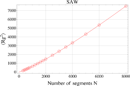
Figure 2: Mean-square radius of gyration for SAW with N𝑁N steps on the cubic lattice. The best estimates of eq. (6) are given by Ξ½=0.5899Β±0.0004𝜈plus-or-minus0.58990.0004\nu=0.5899\pm 0.0004, A=0.187Β±0.001𝐴plus-or-minus0.1870.001A=0.187\pm 0.001 and B=βˆ’3.0Β±0.9𝐡plus-or-minus3.00.9B=-3.0\pm 0.9. The Ο‡2superscriptπœ’2\chi^{2}-value per datum is given by 0.94.

The mean-square radius of gyration, Rg2superscriptsubscript𝑅𝑔2R_{g}^{2}, for SAW on the cubic lattice is evaluated for several different numbers of N𝑁N. The fitting curve in Fig. 2 is given by

Rg2=A​N2​ν​(1+B/N).superscriptsubscript𝑅𝑔2𝐴superscript𝑁2𝜈1𝐡𝑁R_{g}^{2}=AN^{2\nu}(1+B/N)\,. (6)

Here the estimate of exponent ν𝜈\nu is given by ν=0.5899±0.0004𝜈plus-or-minus0.58990.0004\nu=0.5899\pm 0.0004, which is consistent with exponent νSAWsubscript𝜈SAW\nu_{\rm SAW} of SAW.

2.2 Distance between two vertices of SAW

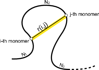
For a given three-dimensional configuration of SAW with N𝑁N steps on the cubic lattice, we take a pair of integers i𝑖i and j𝑗j such that 0≀i<j≀N0𝑖𝑗𝑁0\leq i<j\leq N (see, Fig. 3). There are N+1𝑁1N+1 vertices in total from the 0th to the N𝑁Nth vertex with position vectors Rβ†’jsubscript→𝑅𝑗{\vec{R}}_{j} for j=0,1,…,N𝑗01…𝑁j=0,1,\ldots,N. To the given configuration of SAW we calculate the distance between the i𝑖ith and j𝑗jth vertices

r​(i,j)=|Rβ†’jβˆ’Rβ†’i|.π‘Ÿπ‘–π‘—subscript→𝑅𝑗subscript→𝑅𝑖r(i,j)=|{\vec{R}}_{j}-{\vec{R}}_{i}|. (7)

We shall denote r​(i,j)π‘Ÿπ‘–π‘—r(i,j) also by ri,jsubscriptπ‘Ÿπ‘–π‘—r_{i,j}, briefly.

For integers i𝑖i and j𝑗j satisfying 1≀i<j≀N1𝑖𝑗𝑁1\leq i<j\leq N, let N1subscript𝑁1N_{1}, N2subscript𝑁2N_{2} and N3subscript𝑁3N_{3} denote the number of steps in the first, second and third part of an N𝑁N-step SAW, respectively, as shown in Fig. 3. We have N1=isubscript𝑁1𝑖N_{1}=i, N2=jβˆ’isubscript𝑁2𝑗𝑖N_{2}=j-i, and N3=Nβˆ’jsubscript𝑁3𝑁𝑗N_{3}=N-j.

Refer to caption
Figure 3: Distance r​(i,j)π‘Ÿπ‘–π‘—r(i,j) between the i𝑖ith and j𝑗jth vertices of a long Self-Avoiding Walk (SAW) of N𝑁N steps, where 1≀i<j≀N1𝑖𝑗𝑁1\leq i<j\leq N and N≫1much-greater-than𝑁1N\gg 1. We have p1​(r,N)subscript𝑝1π‘Ÿπ‘p_{1}(r,N) for N1=0subscript𝑁10N_{1}=0 and N2β‰ˆN/2subscript𝑁2𝑁2N_{2}\approx N/2, and p2​(r,N)subscript𝑝2π‘Ÿπ‘p_{2}(r,N) for N1,N2,N3≫1much-greater-thansubscript𝑁1subscript𝑁2subscript𝑁31N_{1},N_{2},N_{3}\gg 1 [29]. We define parameter Ξ»πœ†\lambda by N2=λ​Nsubscript𝑁2πœ†π‘N_{2}=\lambda N and parameter ΞΌπœ‡\mu by N1=μ​λ​Nsubscript𝑁1πœ‡πœ†π‘N_{1}=\mu\lambda N.

We denote by RN​(i,j)subscript𝑅𝑁𝑖𝑗R_{N}(i,j) the average distance between the i𝑖ith and j𝑗jth vertices of an N-step SAW, i.e. the square root of the mean square distance between the i𝑖ith and j𝑗jth vertices of SAW with N𝑁N steps: RN​(i,j)=⟨ri​j2⟩subscript𝑅𝑁𝑖𝑗delimited-⟨⟩subscriptsuperscriptπ‘Ÿ2𝑖𝑗R_{N}(i,j)=\sqrt{\langle r^{2}_{ij}\rangle}. It is approximated by

(RN​(i,j))2=Ai,j​|jβˆ’i|2​ν​(1+Bi,j/|jβˆ’i|).superscriptsubscript𝑅𝑁𝑖𝑗2subscript𝐴𝑖𝑗superscript𝑗𝑖2𝜈1subscript𝐡𝑖𝑗𝑗𝑖\left(R_{N}(i,j)\right)^{2}=A_{i,j}|j-i|^{2\nu}\left(1+B_{i,j}/|j-i|\right)\,. (8)

Here Ai,jsubscript𝐴𝑖𝑗A_{i,j} and Bi,jsubscript𝐡𝑖𝑗B_{i,j} are fitting parameters.

We introduce parameter Ξ»πœ†\lambda such that selected two points i𝑖i and j𝑗j are separated by λ​Nπœ†π‘\lambda N steps (0≀λ≀10πœ†10\leq\lambda\leq 1): N2=λ​Nsubscript𝑁2πœ†π‘N_{2}=\lambda N. We define parameter ΞΌπœ‡\mu by N1=μ​N2subscript𝑁1πœ‡subscript𝑁2N_{1}=\mu N_{2}. We have

N1=μ​N2=μ​λ​N.subscript𝑁1πœ‡subscript𝑁2πœ‡πœ†π‘N_{1}=\mu N_{2}=\mu\lambda N\,. (9)

In terms of parameters Ξ»πœ†\lambda and ΞΌπœ‡\mu, integers i𝑖i and j𝑗j are given by i=N1=μ​λ​N𝑖subscript𝑁1πœ‡πœ†π‘i=N_{1}=\mu\lambda N and j=N1+N2=(1+ΞΌ)​λ​N𝑗subscript𝑁1subscript𝑁21πœ‡πœ†π‘j=N_{1}+N_{2}=(1+\mu)\lambda N, respectively. The intger N3subscript𝑁3N_{3} is givben by N3=Nβˆ’j=Nβˆ’(1+ΞΌ)​λ​Nsubscript𝑁3𝑁𝑗𝑁1πœ‡πœ†π‘N_{3}=N-j=N-(1+\mu)\lambda N. In the case of s=2𝑠2s=2 where N1=N3subscript𝑁1subscript𝑁3N_{1}=N_{3}, we have (1+2​μ)​λ=112πœ‡πœ†1(1+2\mu)\lambda=1.

Refer to caption
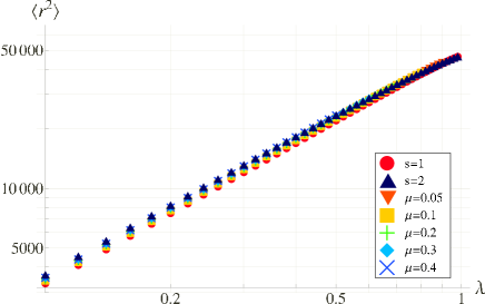
Figure 4: The mean-square distance, RN2​(i,j)=⟨ri,j2⟩superscriptsubscript𝑅𝑁2𝑖𝑗delimited-⟨⟩subscriptsuperscriptπ‘Ÿ2𝑖𝑗R_{N}^{2}(i,j)=\langle r^{2}_{i,j}\rangle, between two points i𝑖i and j𝑗j separated by λ​Nπœ†π‘\lambda N steps in a SAW of N𝑁N steps on the cubic lattice, where jβˆ’i=λ​Nπ‘—π‘–πœ†π‘j-i=\lambda N and i=μ​λ​Nπ‘–πœ‡πœ†π‘i=\mu\lambda N for ΞΌπœ‡\mu = 0, 0.05, 0.1, 0.2, 0.3, and 0.4. Here N=8000𝑁8000N=8000. The case of s=1𝑠1s=1 corresponds to ΞΌ=0πœ‡0\mu=0.

The data of the mean square distance ⟨ri,j2⟩delimited-⟨⟩subscriptsuperscriptπ‘Ÿ2𝑖𝑗\langle r^{2}_{i,j}\rangle versus Ξ»πœ†\lambda are shown in Fig. 4. The data points of different values of parameter ΞΌπœ‡\mu almost coincide each other for 0≀μ≀0.50πœ‡0.50\leq\mu\leq 0.5 in Fig. 4. It is thus suggested that the fitting parameters of (8) are continuous with respect to the change of parameter ΞΌπœ‡\mu.

ν𝜈\nu Ai,jsubscript𝐴𝑖𝑗A_{i,j} Bi,jsubscript𝐡𝑖𝑗B_{i,j}
s=1𝑠1s=1 0.589 Β±0.0007plus-or-minus0.0007\pm 0.0007 1.26 Β±0.02plus-or-minus0.02\pm 0.02 -3 Β±2plus-or-minus2\pm 2
ΞΌ=0.05πœ‡0.05\mu=0.05 0.5888 Β±0.0009plus-or-minus0.0009\pm 0.0009 1.29 Β±0.02plus-or-minus0.02\pm 0.02 βˆ’3Β±3plus-or-minus33-3\pm 3
ΞΌ=0.1πœ‡0.1\mu=0.1 0.5877 Β±0.0008plus-or-minus0.0008\pm 0.0008 1.33 Β±0.02plus-or-minus0.02\pm 0.02 βˆ’6Β±3plus-or-minus63-6\pm 3
ΞΌ=0.2πœ‡0.2\mu=0.2 0.5881 Β±0.001plus-or-minus0.001\pm 0.001 1.34 Β±0.02plus-or-minus0.02\pm 0.02 βˆ’5Β±3plus-or-minus53-5\pm 3
ΞΌ=0.3πœ‡0.3\mu=0.3 0.589 Β±0.001plus-or-minus0.001\pm 0.001 1.34 Β±0.03plus-or-minus0.03\pm 0.03 βˆ’2Β±4plus-or-minus24-2\pm 4
ΞΌ=0.4πœ‡0.4\mu=0.4 0.585 Β±0.003plus-or-minus0.003\pm 0.003 1.45 Β±0.06plus-or-minus0.06\pm 0.06 βˆ’16Β±8plus-or-minus168-16\pm 8
s=2𝑠2s=2 0.562 Β±0.001plus-or-minus0.001\pm 0.001 2.13 Β±0.05plus-or-minus0.05\pm 0.05 -52 Β±4plus-or-minus4\pm 4
Table 1: Estimates of parameters for the graph of the mean-square diatance of two points of SAW separated by λ​Nπœ†π‘\lambda N steps versus parameter Ξ»πœ†\lambda: ⟨r2​(i,j)⟩=Ai,j​(λ​N)2​ν​(1+Bi,j/(λ​N))delimited-⟨⟩superscriptπ‘Ÿ2𝑖𝑗subscript𝐴𝑖𝑗superscriptπœ†π‘2𝜈1subscriptπ΅π‘–π‘—πœ†π‘\langle r^{2}(i,j)\rangle=A_{i,j}(\lambda N)^{2\nu}(1+B_{i,j}/(\lambda N)) where jβˆ’i=λ​Nπ‘—π‘–πœ†π‘j-i=\lambda N, i=μ​λ​Nπ‘–πœ‡πœ†π‘i=\mu\lambda N and 0.1≀λ≀0.50.1πœ†0.50.1\leq\lambda\leq 0.5. Here N=8,000𝑁8000N=8,000.

We consider two special types of interchain distance: RN,s​(Ξ»)subscriptπ‘…π‘π‘ πœ†R_{N,s}(\lambda) for s=1,2𝑠12s=1,2. We define RN,1​(Ξ»)subscript𝑅𝑁1πœ†R_{N,1}(\lambda) by the square root of the mean-square distance between the 0th and λ​Nπœ†π‘\lambda Nth vertices. Here we recall i=0𝑖0i=0 and j=λ​Nπ‘—πœ†π‘j=\lambda N: RN,1​(Ξ»)=⟨r2​(0,λ​N)⟩subscript𝑅𝑁1πœ†delimited-⟨⟩superscriptπ‘Ÿ20πœ†π‘R_{N,1}(\lambda)=\sqrt{\left\langle r^{2}(0,\lambda N)\right\rangle}. We define RN,2​(Ξ»)subscript𝑅𝑁2πœ†R_{N,2}(\lambda) by the square root of the mean-square distance between the (1Β±Ξ»)​N/2plus-or-minus1πœ†π‘2(1\pm\lambda)N/2 th vertices. Here, we have i=(1βˆ’Ξ»)​N/2𝑖1πœ†π‘2i=(1-\lambda)N/2 and j=(1+Ξ»)​N/2𝑗1πœ†π‘2j=(1+\lambda)N/2, and parameter ΞΌπœ‡\mu is given by ΞΌ=(1βˆ’Ξ»)/(2​λ)πœ‡1πœ†2πœ†\mu=(1-\lambda)/(2\lambda). Thus, we have RN,2​(Ξ»)=⟨r2​((1βˆ’Ξ»)​N/2,(1+Ξ»)​N/2)⟩subscript𝑅𝑁2πœ†delimited-⟨⟩superscriptπ‘Ÿ21πœ†π‘21πœ†π‘2R_{N,2}(\lambda)=\sqrt{\left\langle r^{2}((1-\lambda)N/2,(1+\lambda)N/2)\right\rangle}. The square roots of interchain distances RN,s​(Ξ»)subscriptπ‘…π‘π‘ πœ†R_{N,s}(\lambda) for s=1,2𝑠12s=1,2 are well approximated by

(RN,s​(Ξ»))2=As​(λ​N)2​ν​(1+Bs/(λ​N)),superscriptsubscriptπ‘…π‘π‘ πœ†2subscript𝐴𝑠superscriptπœ†π‘2𝜈1subscriptπ΅π‘ πœ†π‘\left(R_{N,s}(\lambda)\right)^{2}=A_{s}(\lambda N)^{2\nu}\left(1+B_{s}/(\lambda N)\right), (10)

where Assubscript𝐴𝑠A_{s} and Bssubscript𝐡𝑠B_{s} are fitting parameters. We shall often neglect the correction term Bs/(λ​N)subscriptπ΅π‘ πœ†π‘B_{s}/(\lambda N).

2.3 Probability distribution function of the distance between two vertices of SAW

Let us denote by p​(𝒓;i,j;N)​d3​𝒓𝑝𝒓𝑖𝑗𝑁superscript𝑑3𝒓p({\mbox{\boldmath$r$}};i,j;N)d^{3}{\mbox{\boldmath$r$}} the probability of finding the j𝑗jth vertex in the region d3​𝒓superscript𝑑3𝒓d^{3}{\mbox{\boldmath$r$}} at a position 𝒓𝒓r from the i𝑖ith vertex of an N𝑁N-step SAW. It is expressed in terms of the average over all configurations of SAW, βŸ¨β‹―βŸ©delimited-βŸ¨βŸ©β‹―\langle\cdots\rangle, as follows.

p​(𝒓;i,j;N)=βŸ¨Ξ΄β€‹(π’“βˆ’(𝑹jβˆ’π‘Ήi))⟩.𝑝𝒓𝑖𝑗𝑁delimited-βŸ¨βŸ©π›Ώπ’“subscript𝑹𝑗subscript𝑹𝑖p({\mbox{\boldmath$r$}};i,j;N)=\langle\delta({\mbox{\boldmath$r$}}-({\mbox{\boldmath$R$}}_{j}-{\mbox{\boldmath$R$}}_{i}))\rangle. (11)

Here we recall that 𝑹isubscript𝑹𝑖{\mbox{\boldmath$R$}}_{i} and 𝑹jsubscript𝑹𝑗{\mbox{\boldmath$R$}}_{j} are the position vectors of the i𝑖ith and j𝑗jth vertices of the SAW, respectively. Due to the rotational symmetry, the probability distribution function p​(𝒓;i,j;N)𝑝𝒓𝑖𝑗𝑁p({\mbox{\boldmath$r$}};i,j;N) depends only on the distance r=|𝒓|π‘Ÿπ’“r=|{\mbox{\boldmath$r$}}|, and we denote it simply by p​(r;i,j;N)π‘π‘Ÿπ‘–π‘—π‘p(r;i,j;N).

We shall show that good fitting curves are given by the following formula

p​(r;i,j;N)=ci,j​(r/RN​(i,j))θ​(i,j)​exp⁑(βˆ’(Di,j​r/RN​(i,j))Ξ΄).π‘π‘Ÿπ‘–π‘—π‘subscript𝑐𝑖𝑗superscriptπ‘Ÿsubscriptπ‘…π‘π‘–π‘—πœƒπ‘–π‘—superscriptsubscriptπ·π‘–π‘—π‘Ÿsubscript𝑅𝑁𝑖𝑗𝛿p(r;i,j;N)=c_{i,j}\,\left(r/R_{N}(i,j)\right)^{\theta(i,j)}\exp\left(-(D_{i,j}\,r/R_{N}(i,j))^{\delta}\right)\,. (12)

Here exponent δ𝛿\delta is related to the exponent ν𝜈\nu by Ξ΄=1/(1βˆ’Ξ½)𝛿11𝜈\delta=1/({1-\nu}), and RN​(i,j)subscript𝑅𝑁𝑖𝑗R_{N}(i,j) are given by the square root of the mean-square distance between the two vertices i𝑖i and j𝑗j. Applying it to the numerical data of p​(r;i,j;N)π‘π‘Ÿπ‘–π‘—π‘p(r;i,j;N), we evaluate exponents θ​(i,j)πœƒπ‘–π‘—\theta(i,j) by the best estimates of parameters for fitting curves.

Let us consider two special types of the probability distribution functions of the distance rπ‘Ÿr between two vertices of an N𝑁N-step SAW: ps​(r;Ξ»,N)subscriptπ‘π‘ π‘Ÿπœ†π‘p_{s}(r;\lambda,N) for s=1,2𝑠12s=1,2. For s=1𝑠1s=1, p1​(r;Ξ»,N)subscript𝑝1π‘Ÿπœ†π‘p_{1}(r;\lambda,N) is defined for the distance rπ‘Ÿr between the vertex of an end point and another vertex of SAW, say, the n𝑛nth vertex with n=λ​Nπ‘›πœ†π‘n=\lambda N; for s=2𝑠2s=2, p2​(r;Ξ»,N)subscript𝑝2π‘Ÿπœ†π‘p_{2}(r;\lambda,N) is defined for the distance rπ‘Ÿr between the (1βˆ’Ξ»)​N/21πœ†π‘2(1-\lambda)N/2th and (1+Ξ»)​N/21πœ†π‘2(1+\lambda)N/2th vertices of SAW. Here we recall that for s=0𝑠0s=0, the probability distribution function p0​(r;N)subscript𝑝0π‘Ÿπ‘p_{0}(r;N) has been defined for the distance rπ‘Ÿr between two ends of an N𝑁N-step SAW. It corresponds to ps​(r;Ξ»,N)subscriptπ‘π‘ π‘Ÿπœ†π‘p_{s}(r;\lambda,N) for s=1,2𝑠12s=1,2 in the case of Ξ»=1πœ†1\lambda=1.

We shall also show that ps​(r;Ξ»,N)subscriptπ‘π‘ π‘Ÿπœ†π‘p_{s}(r;\lambda,N) for s=1,2𝑠12s=1,2 are well approximated by

ps​(r;Ξ»,N)=cs​(r/RN,s​(Ξ»))ΞΈs​(Ξ»)​exp⁑(βˆ’(Ds​r/RN,s​(Ξ»))Ξ΄).subscriptπ‘π‘ π‘Ÿπœ†π‘subscript𝑐𝑠superscriptπ‘Ÿsubscriptπ‘…π‘π‘ πœ†subscriptπœƒπ‘ πœ†superscriptsubscriptπ·π‘ π‘Ÿsubscriptπ‘…π‘π‘ πœ†π›Ώp_{s}(r;\lambda,N)=c_{s}\,\left(r/R_{N,s}(\lambda)\right)^{\theta_{s}(\lambda)}\exp\left(-(D_{s}\,r/R_{N,s}(\lambda))^{\delta}\right)\,. (13)

We shall evaluate exponents ΞΈs​(Ξ»)subscriptπœƒπ‘ πœ†\theta_{s}(\lambda) for s=1,2𝑠12s=1,2 by the fitting formula of ps​(r;Ξ»,N)subscriptπ‘π‘ π‘Ÿπœ†π‘p_{s}(r;\lambda,N) for s=1,2𝑠12s=1,2, respectively.

2.4 Distribution function of the normalized distance

Let us assume an ensemble of SAW where there are W=105π‘Šsuperscript105W=10^{5} random configurations of N𝑁N-step SAW on the cubic lattice. For the distance between the i𝑖ith and j𝑗jth vertices, ri,jsubscriptπ‘Ÿπ‘–π‘—r_{i,j}, we introduce the normalized distance xi,jsubscriptπ‘₯𝑖𝑗x_{i,j} by

xi,j=ri,j/⟨ri,j2⟩.subscriptπ‘₯𝑖𝑗subscriptπ‘Ÿπ‘–π‘—delimited-⟨⟩superscriptsubscriptπ‘Ÿπ‘–π‘—2x_{i,j}=r_{i,j}/\sqrt{\langle r_{i,j}^{2}\rangle}. (14)

We set the length Δ​xΞ”π‘₯\Delta x of intervals by Δ​x=10βˆ’1Ξ”π‘₯superscript101\Delta x=10^{-1}. We enumerate the number of configurations of SAW such that the normalized distance xi,jsubscriptπ‘₯𝑖𝑗x_{i,j} between the i𝑖ith and j𝑗jth vertices satisfies the conditions x<xi​j<x+Δ​xπ‘₯subscriptπ‘₯𝑖𝑗π‘₯Ξ”π‘₯x<x_{ij}<x+\Delta x. We express the number by ni​j​(x,Δ​x)subscript𝑛𝑖𝑗π‘₯Ξ”π‘₯n_{ij}(x,\Delta x). We define the probability distribution function f​(x;i,j;N)𝑓π‘₯𝑖𝑗𝑁f(x;i,j;N) of the normalized distance xπ‘₯x between the i𝑖ith and j𝑗jth vertices by

x2​f​(x;i,j;N)​Δ​x=ni​j​(x,Δ​x)/W.superscriptπ‘₯2𝑓π‘₯𝑖𝑗𝑁Δπ‘₯subscript𝑛𝑖𝑗π‘₯Ξ”π‘₯π‘Šx^{2}f(x;i,j;N)\Delta x=n_{ij}(x,\Delta x)/W\,. (15)

In terms of p​(r;i,j;N)π‘π‘Ÿπ‘–π‘—π‘p(r;i,j;N) we have f​(x;i,j;N)=4​π​RN3​(i,j)​p​(r;i,j;N)𝑓π‘₯𝑖𝑗𝑁4πœ‹subscriptsuperscript𝑅3π‘π‘–π‘—π‘π‘Ÿπ‘–π‘—π‘f(x;i,j;N)=4\pi R^{3}_{N}(i,j)\,p(r;i,j;N). Hereafter we also call f​(x;i,j;N)𝑓π‘₯𝑖𝑗𝑁f(x;i,j;N) distribution function.

Let us now introduce symbols fs​(x;Ξ»,N)subscript𝑓𝑠π‘₯πœ†π‘f_{s}(x;\lambda,N) for s=0,1,2𝑠012s=0,1,2. We denote by f0​(x;N)subscript𝑓0π‘₯𝑁f_{0}(x;N) the probability distribution function of the normalized end-to-end distance x=r/RNπ‘₯π‘Ÿsubscript𝑅𝑁x=r/R_{N}. We then denote by f1​(x;Ξ»,N)subscript𝑓1π‘₯πœ†π‘f_{1}(x;\lambda,N) the probability distribution function of the normalized distance between an end point (the 0th vertex) and the λ​Nπœ†π‘\lambda Nth vertex of SAW of N𝑁N steps and by f2​(x;Ξ»,N)subscript𝑓2π‘₯πœ†π‘f_{2}(x;\lambda,N) that of the normalized distance between two vertices separated by λ​Nπœ†π‘\lambda N steps in a middle region of SAW.

2.5 Algorithm for constructing off-lattice SAP

We generated 2Γ—1052superscript1052\times 10^{5} configurations of SAP consisting of N𝑁N cylindrical segments with cylindrical radius re​xsubscriptπ‘Ÿπ‘’π‘₯r_{ex} of unit length for various number of nodes N𝑁N. Each cylinder segment has the excluded volume of π​re​x2πœ‹superscriptsubscriptπ‘Ÿπ‘’π‘₯2\pi r_{ex}^{2}. In the model of cylindrical SAP, we assume that neighboring segments have no excluded volume interaction: Neighboring cylinder segments may overlap each other.

In the Monte-Carlo procedure we first select two nodes of SAP randomly and consider a subchain between the two nodes. We then constructed the ensembles of cylindrical SAP by combinig the crank-shaft move and the rotation of a subchain of cylindrical SAP around an axis at the center of the axis by 180 degrees. Here, the axis is orthogonal to the end-to-end vector of the subchain We apply the crank-shaft move 2​N2𝑁2N times, and then we apply the rotation of subchains 2​N2𝑁2N times in the Monte-Carlo algorithm.

3 Scaling behavior of interchain correlation of SAW

3.1 Distribution functions fs​(x;Ξ»;N)subscript𝑓𝑠π‘₯πœ†π‘f_{s}(x;\lambda;N) of the distance between two vertices of SAW and short-distance exponents ΞΈssubscriptπœƒπ‘ \theta_{s}

Let us introduce the formula for fitting curves to the data of the probability distribution functions fs​(x;Ξ»,N)subscript𝑓𝑠π‘₯πœ†π‘f_{s}(x;\lambda,N) for s=1,2𝑠12s=1,2 as follows.

fs​(x;Ξ»,N)=Cs​xΞΈs​(Ξ»)​exp⁑(βˆ’(Ds​x)Ξ΄)subscript𝑓𝑠π‘₯πœ†π‘subscript𝐢𝑠superscriptπ‘₯subscriptπœƒπ‘ πœ†superscriptsubscript𝐷𝑠π‘₯𝛿f_{s}(x;\lambda,N)=C_{s}\,x^{\theta_{s}(\lambda)}\exp\left(-(D_{s}\,x)^{\delta}\right)\, (16)

where Ξ΄=1/(1βˆ’Ξ½)𝛿11𝜈\delta=1/(1-\nu). The constants Dssubscript𝐷𝑠D_{s} and Cssubscript𝐢𝑠C_{s} are given by

Dssubscript𝐷𝑠\displaystyle D_{s} =\displaystyle= Γ​((5+ΞΈs)/Ξ΄)Γ​((3+ΞΈs)/Ξ΄),Ξ“5subscriptπœƒπ‘ π›ΏΞ“3subscriptπœƒπ‘ π›Ώ\displaystyle\sqrt{\frac{\Gamma((5+\theta_{s})/\delta)}{\Gamma((3+\theta_{s})/\delta)}}\,,
Cssubscript𝐢𝑠\displaystyle C_{s} =\displaystyle= δΓ​((3+ΞΈs)/Ξ΄)​(Γ​((5+ΞΈs)/Ξ΄)Γ​((3+ΞΈs)/Ξ΄))(3+ΞΈs)/Ξ΄.𝛿Γ3subscriptπœƒπ‘ π›ΏsuperscriptΞ“5subscriptπœƒπ‘ π›ΏΞ“3subscriptπœƒπ‘ π›Ώ3subscriptπœƒπ‘ π›Ώ\displaystyle{\frac{\delta}{\Gamma((3+\theta_{s})/\delta)}}\left({\frac{\Gamma((5+\theta_{s})/\delta)}{\Gamma((3+\theta_{s})/\delta)}}\right)^{(3+\theta_{s})/\delta}\,. (17)

Here we recall that xπ‘₯x denotes the normalized distance: x=r/RN,s​(Ξ»)π‘₯π‘Ÿsubscriptπ‘…π‘π‘ πœ†x=r/R_{N,s}(\lambda), where RN,s​(Ξ»)=As​(λ​N)Ξ½subscriptπ‘…π‘π‘ πœ†subscript𝐴𝑠superscriptπœ†π‘πœˆR_{N,s}(\lambda)=\sqrt{A_{s}}\,(\lambda N)^{\nu}. For s=0𝑠0s=0, we assume that RN,s​(Ξ»)subscriptπ‘…π‘π‘ πœ†R_{N,s}(\lambda) denotes the end-to-end distance RNsubscript𝑅𝑁R_{N}, and apply the formula which is obtained by replacing all ΞΈs​(Ξ»)subscriptπœƒπ‘ πœ†\theta_{s}(\lambda) of (16) and (17) with ΞΈ0subscriptπœƒ0\theta_{0}.

Formula (16) has two fitting parameters ΞΈs​(Ξ»)subscriptπœƒπ‘ πœ†\theta_{s}(\lambda) and δ𝛿\delta for each s𝑠s of s=1,2𝑠12s=1,2. The constants Cssubscript𝐢𝑠C_{s} and Dssubscript𝐷𝑠D_{s} satisfy the followng constraints for s=1,2𝑠12s=1,2:

∫0∞x2​fs​(x;Ξ»,N)​𝑑x=1,∫0∞x4​fs​(x;Ξ»,N)​𝑑x=1.formulae-sequencesuperscriptsubscript0superscriptπ‘₯2subscript𝑓𝑠π‘₯πœ†π‘differential-dπ‘₯1superscriptsubscript0superscriptπ‘₯4subscript𝑓𝑠π‘₯πœ†π‘differential-dπ‘₯1\int_{0}^{\infty}x^{2}f_{s}(x;\lambda,N)dx=1\,,\quad\int_{0}^{\infty}x^{4}f_{s}(x;\lambda,N)dx=1\,. (18)

We made the graphs of the distribution function of the end-to-end distance f0​(x;N)subscript𝑓0π‘₯𝑁f_{0}(x;N) (s=0𝑠0s=0) and those of the distribution functions fs​(x;Ξ»,N)subscript𝑓𝑠π‘₯πœ†π‘f_{s}(x;\lambda,N) of the distance between two vertices separated by λ​Nπœ†π‘\lambda N steps for s=1,2𝑠12s=1,2 with 45 different vaues of Ξ»πœ†\lambda from 0.10 to 0.98 by 0.02 against normalized distance xπ‘₯x. Each graph has 20 data points from x=0.05π‘₯0.05x=0.05 to 1.951.951.95. Here we recall that 105superscript10510^{5} SAWs of N𝑁N steps are generated by the pivot algorithm for N=8,000𝑁8000N=8,000.

Refer to caption
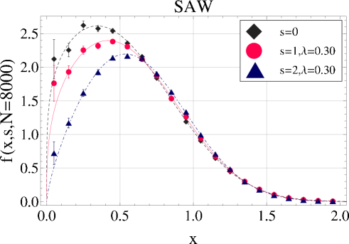
Figure 5: Distribution function fs​(x;Ξ»,N)subscript𝑓𝑠π‘₯πœ†π‘f_{s}(x;\lambda,N) of the distance between two vertices of Self-Avoiding Walk of N𝑁N steps separated by λ​Nπœ†π‘\lambda N steps for s=1,2𝑠12s=1,2, with Ξ»=0.3πœ†0.3\lambda=0.3 and N=8,000𝑁8000N=8,000. Distribution function of the end-to-end distance, f0​(x;N)subscript𝑓0π‘₯𝑁f_{0}(x;N), is also plotted. Each distribution function has 20 data-points.

Formula (16) gives good fitting curves to the data of the probability distribution functions fs​(x;Ξ»,N)subscript𝑓𝑠π‘₯πœ†π‘f_{s}(x;\lambda,N) of the distance between two vertices of SAW for several different values of Ξ»πœ†\lambda and N𝑁N and over almost the entire region of normalized distance xπ‘₯x. The Ο‡2superscriptπœ’2\chi^{2} value per datum is less than 2.0 for all fitting curves (in total, 91 curves).

We have thus shown that the probability distribution function of the distance between two vertices of type s𝑠s (s=0,1,2𝑠012s=0,1,2) is given by

ps​(r;Ξ»,N)=fs​(r/RN,s​(Ξ»);Ξ»,N)/(4​π​RN,s3​(Ξ»)).subscriptπ‘π‘ π‘Ÿπœ†π‘subscriptπ‘“π‘ π‘Ÿsubscriptπ‘…π‘π‘ πœ†πœ†π‘4πœ‹subscriptsuperscript𝑅3π‘π‘ πœ†p_{s}(r;\lambda,N)=f_{s}(r/R_{N,s}(\lambda);\lambda,N)/\left(4\pi R^{3}_{N,s}(\lambda)\right)\,. (19)

where RN,s​(Ξ»)=As​(λ​N)Ξ½subscriptπ‘…π‘π‘ πœ†subscript𝐴𝑠superscriptπœ†π‘πœˆR_{N,s}(\lambda)=\sqrt{A_{s}}(\lambda N)^{\nu} for s=1,2𝑠12s=1,2.

We have evaluated parameters δ​(Ξ»)π›Ώπœ†\delta(\lambda) (or ν​(Ξ»)πœˆπœ†\nu(\lambda)) and ΞΈs​(Ξ»)subscriptπœƒπ‘ πœ†\theta_{s}(\lambda) for s=1,2𝑠12s=1,2 with the least-square method by applying formula (16) to the data plots of the probability distribution functions fs​(x;Ξ»,N)subscript𝑓𝑠π‘₯πœ†π‘f_{s}(x;\lambda,N) for s=1,2𝑠12s=1,2 as functions of normalized distance xπ‘₯x over the entire region of xπ‘₯x for various values of Ξ»πœ†\lambda (0.1<Ξ»<1.0)0.1πœ†1.0(0.1<\lambda<1.0). Here, N=8,000𝑁8000N=8,000. For a given value of Ξ»πœ†\lambda and each of s=1,2𝑠12s=1,2, we make a fitting curve to the data points of distribution function fs​(x;Ξ»,N)subscript𝑓𝑠π‘₯πœ†π‘f_{s}(x;\lambda,N) of the distance between two vertices, and evaluate fitting parameters δ​(Ξ»)π›Ώπœ†\delta(\lambda) and ΞΈs​(Ξ»)subscriptπœƒπ‘ πœ†\theta_{s}(\lambda).

Refer to caption
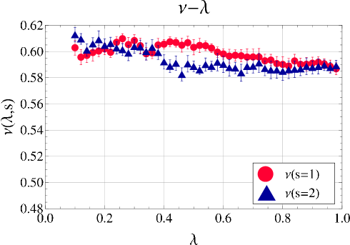
Figure 6: Exponents ν​(Ξ»)πœˆπœ†\nu(\lambda) evaluated through the distribution functions fs​(x;Ξ»,N)subscript𝑓𝑠π‘₯πœ†π‘f_{s}(x;\lambda,N) of the distance between two points separated by λ​Nπœ†π‘\lambda N steps of SAW with N=8,000𝑁8000N=8,000 for 0.1≀λ<10.1πœ†10.1\leq\lambda<1. Here, ν𝜈\nu is calcuted from δ𝛿\delta by Ξ½=1βˆ’1/δ𝜈11𝛿\nu=1-1/\delta.

The estimates of ν​(Ξ»)πœˆπœ†\nu(\lambda) evauated from δ​(Ξ»)π›Ώπœ†\delta(\lambda) in formula (16) of distribution functions fs​(x;Ξ»,N)subscript𝑓𝑠π‘₯πœ†π‘f_{s}(x;\lambda,N) for s=1,2𝑠12s=1,2 via relation Ξ½=1βˆ’1/δ𝜈11𝛿\nu=1-1/\delta, are plotted against parameter Ξ»πœ†\lambda in Fig. 6. They are almost completely constant with respect to Ξ»πœ†\lambda, and consistent with the exponent of SAW, Ξ½SAWβ‰ˆ0.588subscript𝜈SAW0.588\nu_{\rm SAW}\approx 0.588.

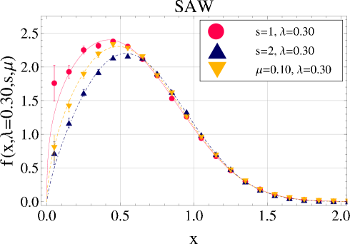
For an illustration, we presented in Fig. 5 fitting curves to distribution functions fs​(x;Ξ»,N)subscript𝑓𝑠π‘₯πœ†π‘f_{s}(x;\lambda,N) for s=1𝑠1s=1 and 2, respectively. In the cases of s=1𝑠1s=1 and 2 the curves for the data-points of Ξ»=0.30πœ†0.30\lambda=0.30 coincide within errors for any value of xπ‘₯x.

s=0𝑠0s=0 s=1𝑠1s=1 s=2𝑠2s=2
Ξ»=0.3πœ†0.3\lambda=0.3 Ξ»=0.3πœ†0.3\lambda=0.3
ΞΈssubscriptπœƒπ‘ \theta_{s} 0.23 Β±0.02plus-or-minus0.02\pm 0.02 0.33 Β±0.03plus-or-minus0.03\pm 0.03 0.73 Β±0.03plus-or-minus0.03\pm 0.03
ν𝜈\nu 0.589 ±0.005plus-or-minus0.005\pm 0.005 0.608 ±0.005plus-or-minus0.005\pm 0.005 0.604 ±0.005plus-or-minus0.005\pm 0.005
Ο‡2superscriptπœ’2\chi^{2}/datum 0.786 0.887 1.07
Table 2: Estimates of fitting parameters and the Ο‡2superscriptπœ’2\chi^{2} value per datum for the fitting curves in Fig. 5: ΞΈs​(Ξ»)subscriptπœƒπ‘ πœ†\theta_{s}(\lambda) and δ𝛿\delta for s=1,2𝑠12s=1,2. Here N=8,000𝑁8000N=8,000 and Ξ»=πœ†absent\lambda= 0.3.

The exponents ΞΈssubscriptπœƒπ‘ \theta_{s} for s=0,1,2𝑠012s=0,1,2 are in increasing order: ΞΈ0<ΞΈ1<ΞΈ2subscriptπœƒ0subscriptπœƒ1subscriptπœƒ2\theta_{0}<\theta_{1}<\theta_{2}. We observe in Fig. 5 that in small xπ‘₯x region, the fitting curve of s=0𝑠0s=0 is higher in position than s=1𝑠1s=1, and the fitting curve of s=1𝑠1s=1 is higher in position than the fitting curve of s=2𝑠2s=2. In fact, by taking the derivative of fitting formula (16), we can show that the peak position of the fitting curve (16) becomes larger as parameter ΞΈssubscriptπœƒπ‘ \theta_{s} increases.

Refer to caption
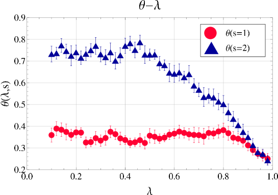
Figure 7: exponents ΞΈ1​(Ξ»)subscriptπœƒ1πœ†\theta_{1}(\lambda) and ΞΈ2​(Ξ»)subscriptπœƒ2πœ†\theta_{2}(\lambda) for 0.1≀λ<10.1πœ†10.1\leq\lambda<1 and N=8,000𝑁8000N=8,000.

The critical exponents ΞΈ1​(Ξ»)subscriptπœƒ1πœ†\theta_{1}(\lambda) and ΞΈ2​(Ξ»)subscriptπœƒ2πœ†\theta_{2}(\lambda) are plotted against parameter Ξ»πœ†\lambda over a wide range such as 0.1≀λ<1.00.1πœ†1.00.1\leq\lambda<1.0 in Fig. 7 for SAW of N=8,000𝑁8000N=8,000 steps. They are given by the best estimates that are obtained by applying formula (16) to the data. Here we recall that formula (16) has only two fitting parameters, ΞΈπœƒ\theta and δ𝛿\delta.

We observe that the estimates of ΞΈ1​(Ξ»)subscriptπœƒ1πœ†\theta_{1}(\lambda) are independent of parameter Ξ»πœ†\lambda for 0.1<Ξ»<0.80.1πœ†0.80.1<\lambda<0.8. The constant value of ΞΈ1​(Ξ»)subscriptπœƒ1πœ†\theta_{1}(\lambda) is given by 0.35 (see also eq. (59), which is a little smaller than the theoretical value: ΞΈ1=0.46subscriptπœƒ10.46\theta_{1}=0.46. Here we remark that in the theoretical derivation [29] the remaining part of the chain is assumed to be infinitely long; i.e., N3β†’βˆžβ†’subscript𝑁3N_{3}\rightarrow\infty. However, when Ξ»<0.8πœ†0.8\lambda<0.8, the remaining part of SAW is more than 20 percentage of the SAW, which may be long enough in the case of N=8,000𝑁8000N=8,000. We also observe that for 0.1<Ξ»<0.50.1πœ†0.50.1<\lambda<0.5, the estimates of ΞΈ2​(Ξ»)subscriptπœƒ2πœ†\theta_{2}(\lambda) do not depend on parameter Ξ»πœ†\lambda, and they are close to the theoretical value: ΞΈ2=0.71subscriptπœƒ20.71\theta_{2}=0.71 with respect to errors, as shown in Fig. 7.

3.2 Distribution functions f​(x;i,j;N)𝑓π‘₯𝑖𝑗𝑁f(x;i,j;N) of the distance between vertices i𝑖i and j𝑗j of SAW and exponent θ​(i,j)πœƒπ‘–π‘—\theta(i,j)

Refer to caption
Figure 8: Distribution functions fs​(x;Ξ»,N)subscript𝑓𝑠π‘₯πœ†π‘f_{s}(x;\lambda,N) with Ξ»=0.30πœ†0.30\lambda=0.30 for s=1,2𝑠12s=1,2, and f​(x;i,j;N)𝑓π‘₯𝑖𝑗𝑁f(x;i,j;N) with i=μ​λ​Nπ‘–πœ‡πœ†π‘i=\mu\lambda N and j=(1+ΞΌ)​λ​N𝑗1πœ‡πœ†π‘j=(1+\mu)\lambda N where Ξ»=0.30πœ†0.30\lambda=0.30 and ΞΌ=0.10πœ‡0.10\mu=0.10, are plotted against normalized distance xπ‘₯x between two vertices. Here N=8,000𝑁8000N=8,000. Each curve has 20 data points with 0.05≀x≀1.950.05π‘₯1.950.05\leq x\leq 1.95.

In Fig. 8 distribution functions fs​(x;Ξ»,N)subscript𝑓𝑠π‘₯πœ†π‘f_{s}(x;\lambda,N) with Ξ»=0.30πœ†0.30\lambda=0.30 and N=8,000𝑁8000N=8,000 for s=1,2𝑠12s=1,2 and distribution function f​(x;i,j;N)𝑓π‘₯𝑖𝑗𝑁f(x;i,j;N) with i=μ​λ​Nπ‘–πœ‡πœ†π‘i=\mu\lambda N and j=(1+ΞΌ)​λ​N𝑗1πœ‡πœ†π‘j=(1+\mu)\lambda N with Ξ»=0.30πœ†0.30\lambda=0.30 and are plotted against normalized distance xπ‘₯x. Here we recall N=8,000𝑁8000N=8,000. In the small xπ‘₯x region, the fitting curve of ΞΌ=0.1πœ‡0.1\mu=0.1 is located between those of s=1𝑠1s=1 and s=2𝑠2s=2. In the large xπ‘₯x region, the three fitting curves overlap each other for s=1,2𝑠12s=1,2 and Ξ»=0.3πœ†0.3\lambda=0.3. We therefore suggest that the asymptotic behavior for large xπ‘₯x is the same among the three cases of fs​(x;Ξ»,N)subscript𝑓𝑠π‘₯πœ†π‘f_{s}(x;\lambda,N) with Ξ»=0.30πœ†0.30\lambda=0.30 for s=1,2𝑠12s=1,2 and f​(x;i,j;N)𝑓π‘₯𝑖𝑗𝑁f(x;i,j;N) with i=μ​λ​Nπ‘–πœ‡πœ†π‘i=\mu\lambda N and j=(1+ΞΌ)​λ​N𝑗1πœ‡πœ†π‘j=(1+\mu)\lambda N with Ξ»=0.30πœ†0.30\lambda=0.30.

In Figs. 7 we observe that as parameter Ξ»πœ†\lambda increases up to Ξ»=1πœ†1\lambda=1 the exponents ΞΈs​(Ξ»)subscriptπœƒπ‘ πœ†\theta_{s}(\lambda) for s=1,2𝑠12s=1,2 are decreasing and become close to the value of exponent ΞΈ0subscriptπœƒ0\theta_{0}. Here we remark that at Ξ»=1πœ†1\lambda=1, the distance between the two vertices is nothing but the end-to-end distance. Therefore, we may expect that the values of exponents ΞΈs​(Ξ»)subscriptπœƒπ‘ πœ†\theta_{s}(\lambda) for s=1,2𝑠12s=1,2 approach the value of ΞΈ0subscriptπœƒ0\theta_{0} when we send Ξ»πœ†\lambda to 1.

Let us now introduce exponent θ​(i,j)πœƒπ‘–π‘—\theta(i,j) in order to describe the short-distance correlation of distribution function f​(x;i,j;N)𝑓π‘₯𝑖𝑗𝑁f(x;i,j;N) for normalized distance xπ‘₯x between the i𝑖ith and j𝑗j th vertices of an N𝑁N-step SAW. We introduce the fitting formula for the distribution functions f​(x;i,j;N)𝑓π‘₯𝑖𝑗𝑁f(x;i,j;N) as follows.

f​(x;i,j;N)=Ci,j​xθ​(i,j)​exp⁑(βˆ’(Di,j​x)Ξ΄)𝑓π‘₯𝑖𝑗𝑁subscript𝐢𝑖𝑗superscriptπ‘₯πœƒπ‘–π‘—superscriptsubscript𝐷𝑖𝑗π‘₯𝛿f(x;i,j;N)=C_{i,j}\,x^{\theta(i,j)}\exp\left(-(D_{i,j}\,x)^{\delta}\right)\, (20)

where Ξ΄=1/(1βˆ’Ξ½)𝛿11𝜈\delta=1/(1-\nu). The constants Di,jsubscript𝐷𝑖𝑗D_{i,j} and Ci,jsubscript𝐢𝑖𝑗C_{i,j} are given by

Di,jsubscript𝐷𝑖𝑗\displaystyle D_{i,j} =\displaystyle= Γ​((5+θ​(i,j))/Ξ΄)Γ​((3+θ​(i,j))/Ξ΄),Ξ“5πœƒπ‘–π‘—π›ΏΞ“3πœƒπ‘–π‘—π›Ώ\displaystyle\sqrt{\frac{\Gamma((5+\theta(i,j))/\delta)}{\Gamma((3+\theta(i,j))/\delta)}}\,,
Ci,jsubscript𝐢𝑖𝑗\displaystyle C_{i,j} =\displaystyle= δΓ​((3+θ​(i,j))/Ξ΄)​(Γ​((5+θ​(i,j))/Ξ΄)Γ​((3+θ​(i,j))/Ξ΄))(3+θ​(i,j))/Ξ΄.𝛿Γ3πœƒπ‘–π‘—π›ΏsuperscriptΞ“5πœƒπ‘–π‘—π›ΏΞ“3πœƒπ‘–π‘—π›Ώ3πœƒπ‘–π‘—π›Ώ\displaystyle{\frac{\delta}{\Gamma((3+\theta(i,j))/\delta)}}\left({\frac{\Gamma((5+\theta(i,j))/\delta)}{\Gamma((3+\theta(i,j))/\delta)}}\right)^{(3+\theta(i,j))/\delta}\,. (21)

Here we recall that xπ‘₯x denotes the normalized distance: x=r/RN​(i,j)π‘₯π‘Ÿsubscript𝑅𝑁𝑖𝑗x=r/R_{N}(i,j), where RN​(i,j)=Ai,j​(λ​N)Ξ½subscript𝑅𝑁𝑖𝑗subscript𝐴𝑖𝑗superscriptπœ†π‘πœˆR_{N}(i,j)=\sqrt{A_{i,j}}\,(\lambda N)^{\nu}.

Let us express vertices i𝑖i and j𝑗j of a SAW in terms of parameters Ξ»πœ†\lambda and ΞΌπœ‡\mu as

i=μ​λ​N,j=(1+ΞΌ)​λ​N.formulae-sequenceπ‘–πœ‡πœ†π‘π‘—1πœ‡πœ†π‘i=\mu\lambda N\,,\quad j=(1+\mu)\lambda N. (22)

If we fix parameter ΞΌπœ‡\mu, vertices i𝑖i and j𝑗j satisfy the following relation

j=i​(1+ΞΌβˆ’1).𝑗𝑖1superscriptπœ‡1j=i\left(1+\mu^{-1}\right)\,. (23)

Here we recall that for a pair of vertices i𝑖i and j𝑗j of a SAW, the numbers N1subscript𝑁1N_{1} and N2subscript𝑁2N_{2} are expressed in terms of parameters Ξ»πœ†\lambda and ΞΌπœ‡\mu by N1=μ​λ​Nsubscript𝑁1πœ‡πœ†π‘N_{1}=\mu\,\lambda N and N2=λ​Nsubscript𝑁2πœ†π‘N_{2}=\lambda N, as shown in Fig. 3.

Refer to caption
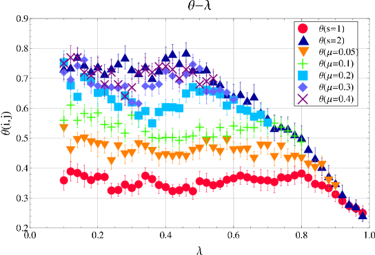
Figure 9: Exponents θ​(i,j)πœƒπ‘–π‘—\theta(i,j) for the distance between the two points separated by λ​Nπœ†π‘\lambda N steps where one point is located at μ​λ​Nπœ‡πœ†π‘\mu\lambda N steps from an end point of SAW, i.e. N1=μ​λ​Nsubscript𝑁1πœ‡πœ†π‘N_{1}=\mu\lambda N. Here, N=8,000𝑁8000N=8,000.

We now show numerically that for a given value of ΞΌπœ‡\mu exponent θ​(i,j)πœƒπ‘–π‘—\theta(i,j) is constant with respect to parameter Ξ»πœ†\lambda on the straight line segment: 0≀λ≀1/(1+2​μ)0πœ†112πœ‡0\leq\lambda\leq 1/(1+2\mu). In Fig. 9 we observe that for given values of parameter ΞΌπœ‡\mu such as 0.05, 0.1, 0.2, 0.3, 0.4, estimates of exponents θ​(i,j)πœƒπ‘–π‘—\theta(i,j) are independent of parameter Ξ»πœ†\lambda for 0.1<Ξ»<0.50.1πœ†0.50.1<\lambda<0.5.

Furthermore, in Fig. 9 we observe crossover phenomenon such that if one of the two points separated by λ​Nπœ†π‘\lambda N steps along SAW is close to an end point of SAW with less than 0.4​λ​N0.4πœ†π‘0.4\lambda N (or 0.5​λ​N0.5πœ†π‘0.5\lambda N) steps (i.e. ΞΌ<0.4πœ‡0.4\mu<0.4 or ΞΌ<0.5πœ‡0.5\mu<0.5), then the value of exponent θ​(i,j)πœƒπ‘–π‘—\theta(i,j) changes from ΞΈ2subscriptπœƒ2\theta_{2} to ΞΈ1subscriptπœƒ1\theta_{1} as parameter ΞΌπœ‡\mu approaches 0.

3.3 Contour plot of exponents θ​(i,j)πœƒπ‘–π‘—\theta(i,j)

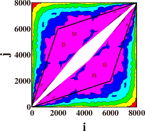
Let us now show that exponent θ​(i,j)πœƒπ‘–π‘—\theta(i,j) as a function of i𝑖i and j𝑗j has a simple structure. The contours of exponent θ​(i,j)πœƒπ‘–π‘—\theta(i,j) are shown in Fig. 10. The region where exponents θ​(i,j)πœƒπ‘–π‘—\theta(i,j) are larger than 0.7 and less than 0.8 is colored by mazenta. The mazenta region of θ​(i,j)πœƒπ‘–π‘—\theta(i,j) satisfying 0.7≀θ​(i,j)<0.80.7πœƒπ‘–π‘—0.80.7\leq\theta(i,j)<0.8 is approximately given by a rhombus with four black edges in Fig. 10. We thus observe that the contour plot of θ​(i,j)πœƒπ‘–π‘—\theta(i,j) has a plateau region of θ​(i,j)β‰ˆΞΈ2πœƒπ‘–π‘—subscriptπœƒ2\theta(i,j)\approx\theta_{2} on the rohmbus in Fig. 10.

The contour plot of Fig. 10 clearly illustrate the following two observations: (i) In Fig. 9 we observe that exponent θ​(i,j)πœƒπ‘–π‘—\theta(i,j) does not depend on parameter Ξ»πœ†\lambda in the region 0≀λ≀1/(1+2​μ)0πœ†112πœ‡0\leq\lambda\leq 1/(1+2\mu); (ii) In Fig. 9 we observe crossover phenomenon: from ΞΈ2subscriptπœƒ2\theta_{2} to ΞΈ1subscriptπœƒ1\theta_{1} as ΞΌπœ‡\mu approaches 0, and then from ΞΈ1subscriptπœƒ1\theta_{1} to ΞΈ0subscriptπœƒ0\theta_{0} as Ξ»πœ†\lambda approaches 1.0.

The graph of (i,j)𝑖𝑗(i,j) for paramter Ξ»πœ†\lambda satisfying 0≀λ≀1/(1+2​μ)0πœ†112πœ‡0\leq\lambda\leq 1/(1+2\mu) is given by the straight line with gradient 1+ΞΌβˆ’11superscriptπœ‡11+\mu^{-1} from the origin (0,0) to the crossing point (ic,jc)subscript𝑖𝑐subscript𝑗𝑐(i_{c},j_{c}) in the graph of i+j=N𝑖𝑗𝑁i+j=N. The crossing point (ic,jc)subscript𝑖𝑐subscript𝑗𝑐(i_{c},j_{c}) is given by

(ic,jc)=(μ​N1+2​μ,(1+ΞΌ)​N1+2​μ).subscript𝑖𝑐subscriptπ‘—π‘πœ‡π‘12πœ‡1πœ‡π‘12πœ‡(i_{c},j_{c})=({\frac{\mu N}{1+2\mu}},{\frac{(1+\mu)N}{1+2\mu}}). (24)

In Fig. 10 we observe that the value of exponent θ​(i,j)πœƒπ‘–π‘—\theta(i,j) is constant on the line segment from the origin to the crossing point (ic,jc)subscript𝑖𝑐subscript𝑗𝑐(i_{c},j_{c}). It depends on parameter ΞΌπœ‡\mu. Here we recall eq. (23).

For instance, the line of ΞΌ=0.5πœ‡0.5\mu=0.5 corresponds to the straight line from the origin (0,0) to (2000, 6000) in the coordinate of (i,j)𝑖𝑗(i,j) with N=8000𝑁8000N=8000. It is given by one of the four edges of the mazenta rohmbus where we have θ​(i,j)β‰ˆΞΈ2πœƒπ‘–π‘—subscriptπœƒ2\theta(i,j)\approx\theta_{2} in Fig. 10. If ΞΌπœ‡\mu becomes smaller than 0.5, then the gradient of the straight line increases and θ​(i,j)πœƒπ‘–π‘—\theta(i,j) becomes smaller than ΞΈ2subscriptπœƒ2\theta_{2}. Finally, we have θ​(i,j)=ΞΈ1πœƒπ‘–π‘—subscriptπœƒ1\theta(i,j)=\theta_{1} at ΞΌ=0πœ‡0\mu=0. Around at the two edges of (0, 8000) and (8000, 0) we have θ​(i,j)=ΞΈ0πœƒπ‘–π‘—subscriptπœƒ0\theta(i,j)=\theta_{0}.

Refer to caption
Figure 10: Exponents θ​(i,j)πœƒπ‘–π‘—\theta(i,j) for 0<i,j<8,000formulae-sequence0𝑖𝑗80000<i,j<8,000. In colored areas with red, yellow, green, cyan, blue, mazenta, and rose pink, we have 0.1Γ—k≀θ​(i,j)<0.1Γ—(k+1)0.1π‘˜πœƒπ‘–π‘—0.1π‘˜10.1\times k\leq\theta(i,j)<0.1\times(k+1) for k=2,3,…,8π‘˜23…8k=2,3,\ldots,8 , respectively. The blank (or empty) region around the diagonal area where |iβˆ’j|𝑖𝑗|i-j| are small has no data due to poor statistics.

We now give an approximate expression for exponent θ​(i,j)πœƒπ‘–π‘—\theta(i,j) as a function of i𝑖i and j𝑗j as follows. For 0≀λ≀1/(1+2​μ)0πœ†112πœ‡0\leq\lambda\leq 1/(1+2\mu) we have

θ​(i,j)={ΞΈ0(M​C)for​μ=0​and​ 0.8<λ≀1.0ΞΈ1(M​C)for​μ=0​and​ 0≀λ≀0.8ΞΈ1(M​C)+4​μ1+2​μ​(ΞΈ2(M​C)βˆ’ΞΈ1(M​C))for​  0<μ≀0.5ΞΈ2(M​C)for​  0.5≀μ<∞.πœƒπ‘–π‘—casessuperscriptsubscriptπœƒ0𝑀𝐢forπœ‡0and0.8πœ†1.0superscriptsubscriptπœƒ1𝑀𝐢forπœ‡0and 0πœ†0.8superscriptsubscriptπœƒ1𝑀𝐢4πœ‡12πœ‡superscriptsubscriptπœƒ2𝑀𝐢superscriptsubscriptπœƒ1𝑀𝐢for  0πœ‡0.5superscriptsubscriptπœƒ2𝑀𝐢for0.5πœ‡\theta(i,j)=\left\{\begin{array}[]{cc}\theta_{0}^{(MC)}&\mbox{for}\,\mu=0\,\mbox{and}\,0.8<\lambda\leq 1.0\\ \theta_{1}^{(MC)}&\mbox{for}\,\mu=0\,\mbox{and}\,0\leq\lambda\leq 0.8\\ \theta_{1}^{(MC)}+\displaystyle{\frac{4\mu}{1+2\mu}}\,(\theta_{2}^{(MC)}-\theta_{1}^{(MC)})&\mbox{for}\,\,0<\mu\leq 0.5\\ \theta_{2}^{(MC)}&\mbox{for}\,\,0.5\leq\mu<\infty\,.\end{array}\right. (25)

Here, estimates ΞΈs(M​C)superscriptsubscriptπœƒπ‘ π‘€πΆ\theta_{s}^{(MC)} for s=0,1,2𝑠012s=0,1,2 are given in eq. (5).

3.4 Correlation functions through exponents θ​(i,j)πœƒπ‘–π‘—\theta(i,j) of SAW

The estimates of short-distance exponents θ​(i,j)πœƒπ‘–π‘—\theta(i,j) shown in Fig. 10 are useful for constructing various quantities of SAW. In fact, formula (20) has only two parameters θ​(i,j)πœƒπ‘–π‘—\theta(i,j)and δ𝛿\delta (or ν𝜈\nu), and the probability distribution function p​(r;i,j;N)π‘π‘Ÿπ‘–π‘—π‘p(r;i,j;N) is determined if we give parameter Ai,jsubscript𝐴𝑖𝑗A_{i,j} (or RN​(i,j)subscript𝑅𝑁𝑖𝑗R_{N}(i,j)) in addition to θ​(i,j)πœƒπ‘–π‘—\theta(i,j) and δ𝛿\delta.

For instance, the pair correlation function of SAW, g​(r)π‘”π‘Ÿg(r), is given by the sum of the distribution functions of the distance between two vertices i𝑖i and j𝑗j, p​(r;i,j;N)π‘π‘Ÿπ‘–π‘—π‘p(r;i,j;N), over all vertices i𝑖i and j𝑗j of SAW.

g​(r)=1Nβ€‹βˆ‘i=1Nβˆ‘j=1Np​(r;i,j;N).π‘”π‘Ÿ1𝑁superscriptsubscript𝑖1𝑁superscriptsubscript𝑗1π‘π‘π‘Ÿπ‘–π‘—π‘g(r)={\frac{1}{N}}\sum_{i=1}^{N}\sum_{j=1}^{N}p(r;i,j;N)\,. (26)

In terms of parameters Ξ»πœ†\lambda and ΞΌπœ‡\mu we have

g​(r)=4​Nβ€‹βˆ«0βˆžπ‘‘ΞΌβ€‹βˆ«01/(1+2​μ)λ​𝑑λ​p​(r;i,j;N).π‘”π‘Ÿ4𝑁superscriptsubscript0differential-dπœ‡superscriptsubscript0112πœ‡πœ†differential-dπœ†π‘π‘Ÿπ‘–π‘—π‘g(r)=4N\int_{0}^{\infty}d\mu\int_{0}^{1/(1+2\mu)}\lambda d\lambda\,p(r;i,j;N)\,. (27)

We define the static structure factor of SAW, g​(𝒒)𝑔𝒒g({\mbox{\boldmath$q$}}), by

g​(𝒒)=1Nβ€‹βˆ‘i=1Nβˆ‘j=1N⟨exp⁑(i​𝒒⋅(𝒓iβˆ’π’“j))⟩.𝑔𝒒1𝑁superscriptsubscript𝑖1𝑁superscriptsubscript𝑗1𝑁delimited-βŸ¨βŸ©β‹…π‘–π’’subscript𝒓𝑖subscript𝒓𝑗g({\mbox{\boldmath$q$}})={\frac{1}{N}}\sum_{i=1}^{N}\sum_{j=1}^{N}\langle\exp\left(i{\mbox{\boldmath$q$}}\cdot({\mbox{\boldmath$r$}}_{i}-{\mbox{\boldmath$r$}}_{j})\right)\rangle. (28)

Assuming the rotational symmetry we have

⟨exp⁑(i​𝒒⋅(𝒓iβˆ’π’“j))⟩=∫0∞sin⁑q​rq​r​p​(r;i,j;N)​ 4​π​r2​𝑑r,delimited-βŸ¨βŸ©β‹…π‘–π’’subscript𝒓𝑖subscript𝒓𝑗superscriptsubscript0π‘žπ‘Ÿπ‘žπ‘Ÿπ‘π‘Ÿπ‘–π‘—π‘4πœ‹superscriptπ‘Ÿ2differential-dπ‘Ÿ\langle\exp\left(i{\mbox{\boldmath$q$}}\cdot({\mbox{\boldmath$r$}}_{i}-{\mbox{\boldmath$r$}}_{j})\right)\rangle=\int_{0}^{\infty}{\frac{\sin qr}{qr}}\,\,p(r;i,j;N)\,4\pi r^{2}dr\,, (29)

where r=|𝒓iβˆ’π’“j|π‘Ÿsubscript𝒓𝑖subscript𝒓𝑗r=|{\mbox{\boldmath$r$}}_{i}-{\mbox{\boldmath$r$}}_{j}| and q=|𝒒|π‘žπ’’q=|{\mbox{\boldmath$q$}}|. We have the following expresion of the static structure factor of SAW:

g​(q)π‘”π‘ž\displaystyle g(q) =\displaystyle= 1Nβ€‹βˆ«0N𝑑mβ€‹βˆ«0N𝑑nβ€‹βˆ«0∞sin⁑q​rq​r​p​(r;m,n;N)​4​π​r2​𝑑r1𝑁superscriptsubscript0𝑁differential-dπ‘šsuperscriptsubscript0𝑁differential-d𝑛superscriptsubscript0π‘žπ‘Ÿπ‘žπ‘Ÿπ‘π‘Ÿπ‘šπ‘›π‘4πœ‹superscriptπ‘Ÿ2differential-dπ‘Ÿ\displaystyle{\frac{1}{N}}\int_{0}^{N}dm\int_{0}^{N}dn\int_{0}^{\infty}{\frac{\sin qr}{qr}}\,p(r;m,n;N)4\pi r^{2}dr (30)
=\displaystyle= 4​Nβ€‹βˆ«0βˆžπ‘‘ΞΌβ€‹βˆ«01/(1+2​μ)Ξ»β€‹π‘‘Ξ»β€‹βˆ«0∞sin⁑q​rq​r​p​(r;Ξ»,ΞΌ;N)​4​π​r2​𝑑r.4𝑁superscriptsubscript0differential-dπœ‡superscriptsubscript0112πœ‡πœ†differential-dπœ†superscriptsubscript0π‘žπ‘Ÿπ‘žπ‘Ÿπ‘π‘Ÿπœ†πœ‡π‘4πœ‹superscriptπ‘Ÿ2differential-dπ‘Ÿ\displaystyle 4N\int_{0}^{\infty}d\mu\int_{0}^{1/(1+2\mu)}\lambda d\lambda\int_{0}^{\infty}{\frac{\sin qr}{qr}}\,p(r;\lambda,\mu;N)4\pi r^{2}dr\,.

Furthermore, the diffusion coefficient of a linear polymer in a good solvent, DG,Lsubscript𝐷𝐺𝐿D_{G,L}, can be evaluated through the probability distribution functions of the distance between two points through the method of Kirkwood’s approximation [24]. In the method DG,Lsubscript𝐷𝐺𝐿D_{G,L} is given by taking the sum of the ensemble average of inverse distance between two points of SAP over all pairs.

DG,L=kB​T6​π​ηs​N2β€‹βˆ‘i=1Nβˆ‘j=1N⟨1|𝒓iβˆ’π’“j|⟩.subscript𝐷𝐺𝐿subscriptπ‘˜π΅π‘‡6πœ‹subscriptπœ‚π‘ superscript𝑁2superscriptsubscript𝑖1𝑁superscriptsubscript𝑗1𝑁delimited-⟨⟩1subscript𝒓𝑖subscript𝒓𝑗D_{G,L}={\frac{k_{B}T}{6\pi\eta_{s}N^{2}}}\sum_{i=1}^{N}\sum_{j=1}^{N}\,\langle{\frac{1}{|{\mbox{\boldmath$r$}}_{i}-{\mbox{\boldmath$r$}}_{j}|}}\rangle\,. (31)

Here Ξ·ssubscriptπœ‚π‘ \eta_{s} denotes the solvent viscosity. We then evaluate the ensemble average of the inverse distance in terms of the probability distribution function, as follows.

DG,Lsubscript𝐷𝐺𝐿\displaystyle D_{G,L} =\displaystyle= kB​T6​π​ηs​N2β€‹βˆ‘i=1Nβˆ‘j=1N∫0∞1r​p​(r;i,j;N)​ 4​π​r2​𝑑rsubscriptπ‘˜π΅π‘‡6πœ‹subscriptπœ‚π‘ superscript𝑁2superscriptsubscript𝑖1𝑁superscriptsubscript𝑗1𝑁superscriptsubscript01π‘Ÿπ‘π‘Ÿπ‘–π‘—π‘4πœ‹superscriptπ‘Ÿ2differential-dπ‘Ÿ\displaystyle{\frac{k_{B}T}{6\pi\eta_{s}N^{2}}}\sum_{i=1}^{N}\sum_{j=1}^{N}\,\int_{0}^{\infty}{\frac{1}{r}}\,p(r;i,j;N)\,4\pi r^{2}dr (32)
=\displaystyle= 4​Nβ€‹βˆ«0βˆžπ‘‘ΞΌβ€‹βˆ«01/(1+2​μ)Ξ»β€‹π‘‘Ξ»β€‹βˆ«0∞1r​p​(r;i,j;N)​ 4​π​r2​𝑑r.4𝑁superscriptsubscript0differential-dπœ‡superscriptsubscript0112πœ‡πœ†differential-dπœ†superscriptsubscript01π‘Ÿπ‘π‘Ÿπ‘–π‘—π‘4πœ‹superscriptπ‘Ÿ2differential-dπ‘Ÿ\displaystyle 4N\int_{0}^{\infty}d\mu\int_{0}^{1/(1+2\mu)}\lambda d\lambda\,\int_{0}^{\infty}\,{\frac{1}{r}}\,p(r;i,j;N)\,4\pi r^{2}dr\,.

4 Scaling behavior of interchain correlation of SAP

4.1 Mean-square radius of gyration for SAP of cylindrical segments under a topological constarint

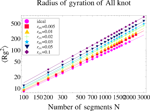
Let us now show the data of the mean-square radius of gyration for cylindrical SAP under a topological constraint of type K𝐾K. We denote it by Rg,K2superscriptsubscript𝑅𝑔𝐾2R_{g,K}^{2}, briefly. Here we recall that SAP consists of N𝑁N cylindrical segments with radius re​xsubscriptπ‘Ÿπ‘’π‘₯r_{ex} of unit length. In Fig. 11 the mean-square radius of gyration of cylindrical SAP under no topological constraint, Rg,A​l​l2superscriptsubscript𝑅𝑔𝐴𝑙𝑙2R_{g,All}^{2}, is plotted for several different values of radius re​xsubscriptπ‘Ÿπ‘’π‘₯r_{ex} with several numbers N𝑁N of segments upto N=3,000𝑁3000N=3,000. The theoretical curves given by the formula Rg2=A​N2​ν​(1+B/N)superscriptsubscript𝑅𝑔2𝐴superscript𝑁2𝜈1𝐡𝑁R_{g}^{2}=AN^{2\nu}(1+B/N) are shown in Fig. 11 together with the data points obtained by simulation. The Ο‡2superscriptπœ’2\chi^{2} values per datum are shown in Table 3. The Ο‡2superscriptπœ’2\chi^{2} values are small in the cases of re​x=0.0subscriptπ‘Ÿπ‘’π‘₯0.0r_{ex}=0.0 (i.e., the ideal case) and re​x=0.10subscriptπ‘Ÿπ‘’π‘₯0.10r_{ex}=0.10. Here, in the latter case the excluded volume has the largest value.

In the case of re​x=0.10subscriptπ‘Ÿπ‘’π‘₯0.10r_{ex}=0.10, the estimate of exponent ν𝜈\nu is numerically close to the exponent of SAW, as shown in Table 3. We suggest that only for the case of re​x=0.10subscriptπ‘Ÿπ‘’π‘₯0.10r_{ex}=0.10, the SAP is long enough so that the excluded volume is fully effective. We shall also confirm it through fitting curves to the distribution functions of the distance between two points in subsection 4.2.
Refer to caption
Figure 11: Double-logarithmic plot of the mean-square radius of gyration of SAP consisting of N𝑁N cylindrical segments with radius re​xsubscriptπ‘Ÿπ‘’π‘₯r_{ex} of unit length under no topological constraint ⟨Rg2⟩A​l​lsubscriptdelimited-⟨⟩superscriptsubscript𝑅𝑔2𝐴𝑙𝑙\langle R_{g}^{2}\rangle_{All}. For the cases of re​xsubscriptπ‘Ÿπ‘’π‘₯r_{ex}= 0.0, 0.05, 0.01, 0.02, 0.03, 0.05 and 0.1 are plotted with purple filled circles, red filled squares, yellow filled triangles, green crosses, light blue stars, dark blue triangles, and purple filled diamonds, respectively.
re​xsubscriptπ‘Ÿπ‘’π‘₯r_{ex} A𝐴A ν𝜈\nu B𝐡B Ο‡2superscriptπœ’2\chi^{2}/datum
0 0.0833 Β±plus-or-minus\pm 0.0004 0.5000 Β±plus-or-minus\pm 0.0003 1.2 Β±0.2plus-or-minus0.2\pm 0.2 1.04
0.005 0.0584 Β±plus-or-minus\pm 0.0006 0.5379 Β±plus-or-minus\pm 0.0008 8.0 Β±0.6plus-or-minus0.6\pm 0.6 7.93
0.01 0.0529 Β±plus-or-minus\pm 0.0006 0.5528 Β±plus-or-minus\pm 0.0007 9.0 Β±0.6plus-or-minus0.6\pm 0.6 7.59
0.02 0.0504 Β±plus-or-minus\pm 0.0005 0.5667 Β±plus-or-minus\pm 0.0006 8.5 Β±0.5plus-or-minus0.5\pm 0.5 7.99
0.05 0.0538 Β±plus-or-minus\pm 0.0003 0.5798 Β±plus-or-minus\pm 0.0003 5.3 Β±0.3plus-or-minus0.3\pm 0.3 2.57
0.1 0.0623 Β±plus-or-minus\pm 0.0003 0.5862 Β±plus-or-minus\pm 0.0004 2.7 Β±0.5plus-or-minus0.5\pm 0.5 0.421
Table 3: Best estimates of the fitting formula: Rg2=A​N2​ν​(1+B/N)superscriptsubscript𝑅𝑔2𝐴superscript𝑁2𝜈1𝐡𝑁R_{g}^{2}=AN^{2\nu}(1+B/N) for the mean-square radius of gyration for SAP consisting of N𝑁N cyllindrical segments with raidus re​xsubscriptπ‘Ÿπ‘’π‘₯r_{ex} of unit length under no topological constraint ⟨Rg2⟩A​l​lsubscriptdelimited-⟨⟩superscriptsubscript𝑅𝑔2𝐴𝑙𝑙\langle R_{g}^{2}\rangle_{All} .

In Fig. 12 the ratio of the mean-square radius of gyration of the cylindrical SAP with the trivial knot (01subscript010_{1}), Rg,012subscriptsuperscript𝑅2𝑔subscript01R^{2}_{g,0_{1}}, to that of under no topological constraint (A​l​l𝐴𝑙𝑙All), Rg,A​l​l2subscriptsuperscript𝑅2𝑔𝐴𝑙𝑙R^{2}_{g,All}, is plotted against the number of nodes N𝑁N for several different values of cylindrical radius re​xsubscriptπ‘Ÿπ‘’π‘₯r_{ex}. The ratio is always larger than 1.0 except for the case of re​x=0.1subscriptπ‘Ÿπ‘’π‘₯0.1r_{ex}=0.1. Furthermore, the ratio decreases as the cylindrical radius increases. Here we remark that the values of Rg,A​l​l2subscriptsuperscript𝑅2𝑔𝐴𝑙𝑙R^{2}_{g,All} for the different values of cylinder radius re​xsubscriptπ‘Ÿπ‘’π‘₯r_{ex} are given in Fig. 11.
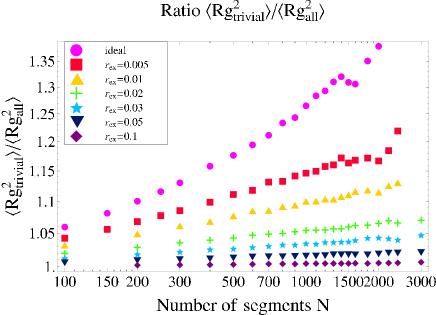
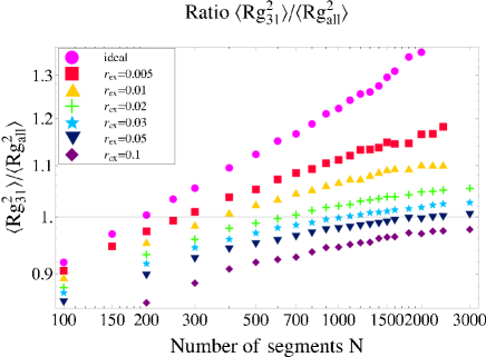
The ratio of the mean-square radius of gyration of the cylindrical SAP with the trefoil knot (31subscript313_{1}), Rg,312subscriptsuperscript𝑅2𝑔subscript31R^{2}_{g,3_{1}}, to that of under notopological constraint, Rg,A​l​l2subscriptsuperscript𝑅2𝑔𝐴𝑙𝑙R^{2}_{g,All}, is plotted in Fig. 13 against the number of nodes N𝑁N for different values of cylindrical radius re​xsubscriptπ‘Ÿπ‘’π‘₯r_{ex}. The ratio is larger than 1.0 for the cases of small values of re​xsubscriptπ‘Ÿπ‘’π‘₯r_{ex} and large N𝑁N. It decreases as the cylindrical radius increases.

Refer to caption
Figure 12: Double-logarithmic plot of the ratio of the mean-square radius of gyration for the N𝑁N-noded SAP with trivial knot (01subscript010_{1}) to that of no topological constraint (including all knots) against the number of nodes N𝑁N for various different values of cylindrical radius re​xsubscriptπ‘Ÿπ‘’π‘₯r_{ex}. Error bars are not shown in the figure.

We thus observe topological swelling in Figs. 12 and 13 [17]. In the cases when the cylindrical radius re​xsubscriptπ‘Ÿπ‘’π‘₯r_{ex} is small, the mean-square radius of gyration of cylindrical SAP with a fixed knot type becomes larger than that of no topological constraint for large enough N𝑁N; i.e., the ratio Rg,K2/Rg,A​l​l2subscriptsuperscript𝑅2𝑔𝐾subscriptsuperscript𝑅2𝑔𝐴𝑙𝑙R^{2}_{g,K}/R^{2}_{g,All} becomes larger than 1.0 if N𝑁N is large enough. Here K𝐾K denotes a knot type. We consider that topological swelling occurs since entropic repulsive forces appear effectively among segments of the SAP under a topological constraint of a fixed knot [38, 17]. Here we remark that the ratios of the mean-square radii of gyration of N𝑁N-noded cylindrical SAP under a topological cnstraint, Rg,K2/Rg,A​l​l2subscriptsuperscript𝑅2𝑔𝐾subscriptsuperscript𝑅2𝑔𝐴𝑙𝑙R^{2}_{g,K}/R^{2}_{g,All}, were evaluated for the trivial and trefoil knots in Ref. [17], although the number of N𝑁N was limited upto N=1,000𝑁1000N=1,000.

We also observe in Fig. 13 that ratio Rg,312/Rg,A​l​l2subscriptsuperscript𝑅2𝑔subscript31subscriptsuperscript𝑅2𝑔𝐴𝑙𝑙R^{2}_{g,3_{1}}/R^{2}_{g,All} is smaller than 1.0 for any value of radius re​xsubscriptπ‘Ÿπ‘’π‘₯r_{ex} if N𝑁N is smaller than 200. It is due to the finite-size effect: The polymer chain is short so that the size of the polymer making the trefoil knot is rather small. However, if the chain is long enough, the necessary number of segments to make the trefoil knot becomes much smaller than the total number of segments N𝑁N, and the rest of the chain becomes as large as SAP of the trivial knot. Therefore, the ratio ⟨Rg,312⟩/⟨Rg,A​l​l2⟩delimited-⟨⟩subscriptsuperscript𝑅2𝑔subscript31delimited-⟨⟩subscriptsuperscript𝑅2𝑔𝐴𝑙𝑙\langle R^{2}_{g,3_{1}}\rangle/\langle R^{2}_{g,All}\rangle, becomes larger than 1.0 for large N𝑁N.

Refer to caption
Figure 13: Double-logarithmic plot of the ratio of the mean-square radius of gyration for the N𝑁N-noded SAP with the treofil knot (31subscript313_{1}) to that of no topological constraint (including all knots) against the number of nodes N𝑁N for various different values of cylindrical radius re​xsubscriptπ‘Ÿπ‘’π‘₯r_{ex}. Error bars are not shown in the figure.

Topological swelling occurs only if the excluded volume is small [33]. For re​x=0.05subscriptπ‘Ÿπ‘’π‘₯0.05r_{ex}=0.05, the ratio ⟨Rg,312⟩/⟨Rg,A​l​l2⟩delimited-⟨⟩subscriptsuperscript𝑅2𝑔subscript31delimited-⟨⟩subscriptsuperscript𝑅2𝑔𝐴𝑙𝑙\langle R^{2}_{g,3_{1}}\rangle/\langle R^{2}_{g,All}\rangle, becomes larger than 1.0 only at N=3,000𝑁3000N=3,000, as shown in Fig. 13. We may therefore consider that the excluded volume effect is not compatible with the topological entropic repulsions among segments of SAP under a topological constraint.

4.2 Probability distribution functions of the distance between two nodes of SAP

Let us consider the probability disrtibution function of the distance between two nodes i𝑖i and j𝑗j of SAP with knot type K𝐾K consisting of N𝑁N cylindrical segments with radius re​xsubscriptπ‘Ÿπ‘’π‘₯r_{ex} and of unit length. We define it by

pK​(𝒓;i,j;N)=βŸ¨Ξ΄β€‹(π’“βˆ’(𝑹jβˆ’π‘Ήi))⟩K.subscript𝑝𝐾𝒓𝑖𝑗𝑁subscriptdelimited-βŸ¨βŸ©π›Ώπ’“subscript𝑹𝑗subscript𝑹𝑖𝐾p_{K}({\mbox{\boldmath$r$}};i,j;N)=\langle\delta({\mbox{\boldmath$r$}}-({\mbox{\boldmath$R$}}_{j}-{\mbox{\boldmath$R$}}_{i}))\rangle_{K}\,. (33)

Here the symbol βŸ¨β‹…βŸ©delimited-βŸ¨βŸ©β‹…\langle\cdot\rangle denotes the average over all possible configurations of cylindrical SAP of N𝑁N nodes havine knot type K𝐾K. For the case of no topological constraint, we denote K𝐾K as All, which suggests that all knots are included.

Due to the cyclic symmetry, the distribution function pK​(𝒓;i,j;N)subscript𝑝𝐾𝒓𝑖𝑗𝑁p_{K}({\mbox{\boldmath$r$}};i,j;N) depends only on the distance |iβˆ’j|𝑖𝑗|i-j|. Let us introduce parameter Ξ»πœ†\lambda for SAP by

Ξ»=|jβˆ’i|/Nπœ†π‘—π‘–π‘\lambda=|j-i|/N (34)

We thus express the probability disrtibution function of the distance between two points i𝑖i and j𝑗j of SAP, as pK​(r;Ξ»,N)subscriptπ‘πΎπ‘Ÿπœ†π‘p_{K}(r;\lambda,N).

Let us denote by RN,K​(Ξ»)subscriptπ‘…π‘πΎπœ†R_{N,K}(\lambda) the square root of the mean square distance between i𝑖i and j𝑗j of N𝑁N-noded SAP with knot type K𝐾K where i𝑖i and j𝑗j are separated by λ​Nπœ†π‘\lambda N steps. It is given by the following:

RN,K​(Ξ»)=⟨ri,j2⟩K.subscriptπ‘…π‘πΎπœ†subscriptdelimited-⟨⟩superscriptsubscriptπ‘Ÿπ‘–π‘—2𝐾R_{N,K}(\lambda)=\sqrt{\langle r_{i,j}^{2}\rangle_{K}}\,. (35)

For the distance between the two nodes i𝑖i and j𝑗j, ri,jsubscriptπ‘Ÿπ‘–π‘—r_{i,j}, we introduce the normalized distance xi,jsubscriptπ‘₯𝑖𝑗x_{i,j} by

xi,j=ri,j/RN,K​(Ξ»).subscriptπ‘₯𝑖𝑗subscriptπ‘Ÿπ‘–π‘—subscriptπ‘…π‘πΎπœ†x_{i,j}=r_{i,j}/R_{N,K}(\lambda)\,. (36)

We denote by fK​(x;Ξ»,N)subscript𝑓𝐾π‘₯πœ†π‘f_{K}(x;\lambda,N) the distribution function of normalized distance xπ‘₯x between two nodes i𝑖i and j𝑗j of N𝑁N-noded SAP with knot K𝐾K consisting of cylindrical segments with radius re​xsubscriptπ‘Ÿπ‘’π‘₯r_{ex}, where i𝑖i and j𝑗j are separated by λ​Nπœ†π‘\lambda N steps. It is expressed in terms of the probability distribution function pK​(r;Ξ»,N)subscriptπ‘πΎπ‘Ÿπœ†π‘p_{K}(r;\lambda,N) as follows.

fK​(x;Ξ»,N)=4​π​RN,K3​(Ξ»)​pK​(x​RN,K;Ξ»,N).subscript𝑓𝐾π‘₯πœ†π‘4πœ‹subscriptsuperscript𝑅3π‘πΎπœ†subscript𝑝𝐾π‘₯subscriptπ‘…π‘πΎπœ†π‘f_{K}(x;\lambda,N)=4\pi R^{3}_{N,K}(\lambda)\,p_{K}(xR_{N,K};\lambda,N)\,. (37)

Here we recall |iβˆ’j|=λ​Nπ‘–π‘—πœ†π‘|i-j|=\lambda N.

Refer to caption
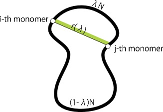
Figure 14: Distance r​(Ξ»)π‘Ÿπœ†r(\lambda) between the i𝑖ith and j𝑗jth vertices of a long Self-Avoiding Polgon (SAP) of N𝑁N steps, where 1≀i<j≀N1𝑖𝑗𝑁1\leq i<j\leq N and N≫1much-greater-than𝑁1N\gg 1. In terms of parameter Ξ»πœ†\lambda we express the difference |iβˆ’j|𝑖𝑗|i-j| as |iβˆ’j|=λ​Nπ‘–π‘—πœ†π‘|i-j|=\lambda N for 0≀λ≀1/20πœ†120\leq\lambda\leq 1/2.

Let us introduce the formula for fitting curves to the data of the probability distribution function of the normalized distance between two segments separated by λ​Nπœ†π‘\lambda N steps, f​(x;Ξ»,N)𝑓π‘₯πœ†π‘f(x;\lambda,N), as follows.

fK​(x;Ξ»,N)=CK​(Ξ»)​xΞΈK​(Ξ»)​exp⁑(βˆ’(DK​x)Ξ΄)subscript𝑓𝐾π‘₯πœ†π‘subscriptπΆπΎπœ†superscriptπ‘₯subscriptπœƒπΎπœ†superscriptsubscript𝐷𝐾π‘₯𝛿f_{K}(x;\lambda,N)=C_{K}(\lambda)\,x^{\theta_{K}(\lambda)}\exp\left(-(D_{K}\,x)^{\delta}\right)\, (38)

where Ξ΄=1/(1βˆ’Ξ½)𝛿11𝜈\delta=1/(1-\nu). The constants D𝐷D and C𝐢C are given by

DKsubscript𝐷𝐾\displaystyle D_{K} =\displaystyle= Γ​((5+ΞΈK)/Ξ΄K)Γ​((3+ΞΈK)/Ξ΄K),Ξ“5subscriptπœƒπΎsubscript𝛿𝐾Γ3subscriptπœƒπΎsubscript𝛿𝐾\displaystyle\sqrt{\frac{\Gamma((5+\theta_{K})/\delta_{K})}{\Gamma((3+\theta_{K})/\delta_{K})}}\,,
CKsubscript𝐢𝐾\displaystyle C_{K} =\displaystyle= δΓ​((3+ΞΈK)/Ξ΄K)​(Γ​((5+ΞΈK)/Ξ΄K)Γ​((3+ΞΈK)/Ξ΄K))(3+ΞΈK)/Ξ΄K.𝛿Γ3subscriptπœƒπΎsubscript𝛿𝐾superscriptΞ“5subscriptπœƒπΎsubscript𝛿𝐾Γ3subscriptπœƒπΎsubscript𝛿𝐾3subscriptπœƒπΎsubscript𝛿𝐾\displaystyle{\frac{\delta}{\Gamma((3+\theta_{K})/\delta_{K})}}\left({\frac{\Gamma((5+\theta_{K})/\delta_{K})}{\Gamma((3+\theta_{K})/\delta_{K})}}\right)^{(3+\theta_{K})/\delta_{K}}\,. (39)

Here we recall that xπ‘₯x denotes the normalized distance: x=r/RN,K​(Ξ»)π‘₯π‘Ÿsubscriptπ‘…π‘πΎπœ†x=r/R_{N,K}(\lambda), where RN,K​(Ξ»)=AK​(λ​N)Ξ½Ksubscriptπ‘…π‘πΎπœ†subscript𝐴𝐾superscriptπœ†π‘subscript𝜈𝐾R_{N,K}(\lambda)=\sqrt{A_{K}}\,(\lambda N)^{\nu_{K}}.

Refer to caption
Figure 15: Estimates of exponent Ξ½A​l​l​(Ξ»)subscriptπœˆπ΄π‘™π‘™πœ†\nu_{All}(\lambda) evaluated by applying formula (38) to the distribution function of the distance between two vertices of SAP with N𝑁N cylindrical segments of radius re​xsubscriptπ‘Ÿπ‘’π‘₯r_{ex} under no topological constraint.

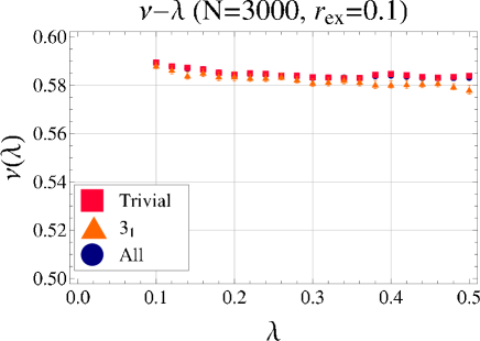
We have evaluated exponent Ξ½K​(Ξ»)subscriptπœˆπΎπœ†\nu_{K}(\lambda) of the N𝑁N-noded cylindrical SAP with topological condition K𝐾K of radius re​xsubscriptπ‘Ÿπ‘’π‘₯r_{ex} for various values of re​xsubscriptπ‘Ÿπ‘’π‘₯r_{ex} such as re​xsubscriptπ‘Ÿπ‘’π‘₯r_{ex}=0, 0.005, 0.01, 0.02, 0.05, and 0.1, and various numbers of N𝑁N such asN𝑁N=400, 800, 1,600, 2,000, 3,000. We have applied formula (38) to the data of the distribution function of the normalized distance between two nodes of the cylindrical SAP, and obtained the best estimates of exponents Ξ΄K​(Ξ»)subscriptπ›ΏπΎπœ†\delta_{K}(\lambda) for each value of Ξ»πœ†\lambda from the fitting curves to the data. We then calculated Ξ½K​(Ξ»)subscriptπœˆπΎπœ†\nu_{K}(\lambda) from the estimates of Ξ΄K​(Ξ»)subscriptπ›ΏπΎπœ†\delta_{K}(\lambda) Here, we have considered the three topoogical conditions, the trivial knot (01subscript010_{1}), the trefoil knot (31subscript313_{1}), and no topological constraint (β€œA​l​l𝐴𝑙𝑙All”), and for 25 values of Ξ»πœ†\lambda from 0.02 to 0.5 by 0.02. The Ο‡2superscriptπœ’2\chi^{2} values per datum are given by less than or equal to 1.0 or 2.0 for all the fitting curves. Thus, we conclude that the fitting curves are good.

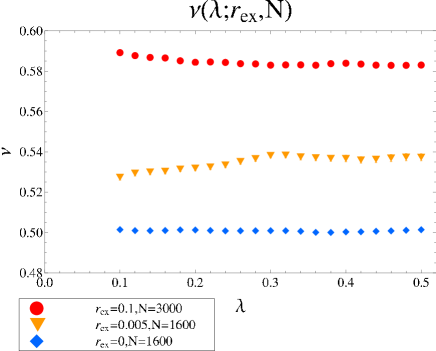
For an illustration, in Fig. 15, the estimates of Ξ½A​l​l​(Ξ»)subscriptπœˆπ΄π‘™π‘™πœ†\nu_{All}(\lambda) with no topological constraint (i.e. K=A​l​l𝐾𝐴𝑙𝑙K=All) are plotted against Ξ»πœ†\lambda for the three cases: the thick case of re​x=0.10subscriptπ‘Ÿπ‘’π‘₯0.10r_{ex}=0.10 and N=3,000𝑁3000N=3,000 (filled red circles), the thin case of re​x=0.005subscriptπ‘Ÿπ‘’π‘₯0.005r_{ex}=0.005 and N=1,600𝑁1600N=1,600 (downward orange triangles) and the ideal case of re​x=0.0subscriptπ‘Ÿπ‘’π‘₯0.0r_{ex}=0.0 and N=1,600𝑁1600N=1,600 (filled dark-blue diamonds). Here we plot the ideal case for reference.

In the thick case (re​x=0.10subscriptπ‘Ÿπ‘’π‘₯0.10r_{ex}=0.10 and N=3,000𝑁3000N=3,000), the value of Ξ½A​l​l​(Ξ»)subscriptπœˆπ΄π‘™π‘™πœ†\nu_{All}(\lambda) is almost consistent with the exponent of SAW, Ξ½S​A​W=0.588subscriptπœˆπ‘†π΄π‘Š0.588\nu_{SAW}=0.588 over all range of Ξ»πœ†\lambda. It is However, in the thin case (re​x=0.005subscriptπ‘Ÿπ‘’π‘₯0.005r_{ex}=0.005 and N=1,600𝑁1600N=1,600), the value of Ξ½A​l​l​(Ξ»)subscriptπœˆπ΄π‘™π‘™πœ†\nu_{All}(\lambda) is rather smaller than the exponent of SAW, Ξ½S​A​Wsubscriptπœˆπ‘†π΄π‘Š\nu_{SAW}. Moreover, in the ideal case (re​x=0.0subscriptπ‘Ÿπ‘’π‘₯0.0r_{ex}=0.0 and N=1,600𝑁1600N=1,600) the estimates of Ξ½A​l​l​(Ξ»)subscriptπœˆπ΄π‘™π‘™πœ†\nu_{All}(\lambda) almost equal to 0.5 for all values of Ξ»πœ†\lambda.

Thus, as far as the excluded volume effect of SAP is concerned, we conclude that for re​x=0.10subscriptπ‘Ÿπ‘’π‘₯0.10r_{ex}=0.10, SAW of N=3,000𝑁3000N=3,000 is large enough to see the effect of excluded volume, while for re​x=0.005subscriptπ‘Ÿπ‘’π‘₯0.005r_{ex}=0.005 and N=1,600𝑁1600N=1,600, SAW of N=1600𝑁1600N=1600 is not large enough to see it.

4.3 Exponents ΞΈK​(Ξ»)subscriptπœƒπΎπœ†\theta_{K}(\lambda) of short-distance correlation of SAP with knot K𝐾K

4.3.1 The case of thick cylindrical SAP
Refer to caption
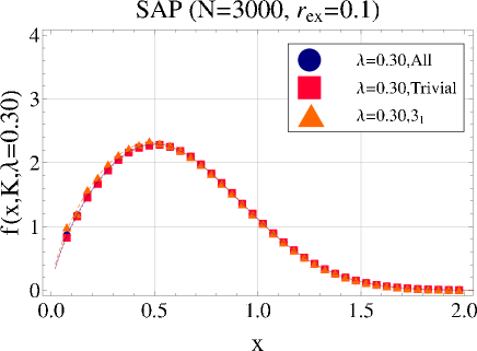
Figure 16: Data points and fittung curves of the distribution functions fK​(x;Ξ»,N)subscript𝑓𝐾π‘₯πœ†π‘f_{K}(x;\lambda,N) of normalized distance xπ‘₯x between two nodes of cylindrical SAP of N=3,000𝑁3000N=3,000 with radius re​x=0.1subscriptπ‘Ÿπ‘’π‘₯0.1r_{ex}=0.1 (thick cylinders) at Ξ»=0.3πœ†0.3\lambda=0.3 for three topological conditions: the trivial knot (01subscript010_{1}), the trefoil knot (31subscript313_{1}) and no toplogical constaint (A​l​l𝐴𝑙𝑙All).

We plotted in Fig. 16 the data points of distibution functions fK​(x;Ξ»,N)subscript𝑓𝐾π‘₯πœ†π‘f_{K}(x;\lambda,N) of normalized distance xπ‘₯x between two nodes of cylindrical SAP of N=3,000𝑁3000N=3,000 consisting of cylindrical segments of radius re​x=0.1subscriptπ‘Ÿπ‘’π‘₯0.1r_{ex}=0.1 of unit length (thick cylinders). Here, the two nodes are separated by λ​Nπœ†π‘\lambda N steps with Ξ»=0.3πœ†0.3\lambda=0.3. We consider three topological conditions: the trivial knot (01subscript010_{1}), the trefoil knot (31subscript313_{1}) and no toplogical constaint (A​l​l𝐴𝑙𝑙All). We recall that the fitting curves are given by formula (38) with two parameters ΞΈKsubscriptπœƒπΎ\theta_{K} and Ξ΄Ksubscript𝛿𝐾\delta_{K}.

K𝐾K No constraint (A​l​l𝐴𝑙𝑙All) trivial knot (00) trefoil knot (31subscript313_{1})
ΞΈKsubscriptπœƒπΎ\theta_{K} 0.664 Β±0.004plus-or-minus0.004\pm 0.004 0.679 Β±0.004plus-or-minus0.004\pm 0.004 0.623 Β±0.009plus-or-minus0.009\pm 0.009
νKsubscript𝜈𝐾\nu_{K} 0.583 ±0.001plus-or-minus0.001\pm 0.001 0.583 ±0.001plus-or-minus0.001\pm 0.001 0.581 ±0.002plus-or-minus0.002\pm 0.002
Ο‡2superscriptπœ’2\chi^{2}/datum 1.19 1.07 1.24
Table 4: Estimates of fitting parameters and the Ο‡2superscriptπœ’2\chi^{2} value per datum for the fitting curves in Fig. 16: re​x=0.1subscriptπ‘Ÿπ‘’π‘₯0.1r_{ex}=0.1, Ξ»=πœ†absent\lambda= 0.3 and N=3000𝑁3000N=3000.

For all the three topological conditions the Ο‡2superscriptπœ’2\chi^{2} values per datum are small. We thus find that the fitting curves to the distribution functions are good. The fitting parameters are listed in Table 4. Here we recall that we have observed in Fig. 11 the excluded volume effect appears clearly for SAP with N=3,000𝑁3000N=3,000 segments in the case of re​x=0.1subscriptπ‘Ÿπ‘’π‘₯0.1r_{ex}=0.1, i.e., the thick cylindrical SAP.

Refer to caption
Figure 17: Estimates of ΞΈK​(Ξ»)subscriptπœƒπΎπœ†\theta_{K}(\lambda) against parameter Ξ»πœ†\lambda for cylindrical SAP with radius re​x=0.1subscriptπ‘Ÿπ‘’π‘₯0.1r_{ex}=0.1 of N=3000𝑁3000N=3000. Here K𝐾K is given by the trivial knot (01subscript010_{1}), the trefoil knot (31subscript313_{1}) and no toplogical constaint (A​l​l𝐴𝑙𝑙All).

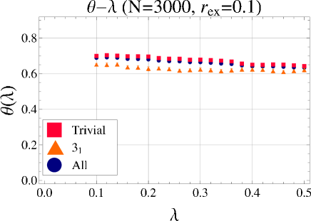
For the thick cylindrical SAP we plotted in Fig. 18 the estimates of exponent ΞΈK​(Ξ»)subscriptπœƒπΎπœ†\theta_{K}(\lambda) against Ξ»πœ†\lambda with 25 values of parameter Ξ»πœ†\lambda for three topological conditions: the trivial knot (01subscript010_{1}), the trefoil knot (31subscript313_{1}) and no toplogical constraint (A​l​l𝐴𝑙𝑙All). All the estimates of exponent ΞΈK​(Ξ»)subscriptπœƒπΎπœ†\theta_{K}(\lambda) are roughly the same such as θ​(Ξ»)β‰ˆ0.7πœƒπœ†0.7\theta(\lambda)\approx 0.7. In each topological condition K𝐾K the estimate of ΞΈK​(Ξ»)subscriptπœƒπΎπœ†\theta_{K}(\lambda) is almost constant with respect to parameter Ξ»πœ†\lambda. Furthermore, they do not depend on topological conditions K𝐾K. The exponent for the trivial knot and the trefoil knot is rather cose to each other, while that of the trefoil knot is smaller than others. that of the : ΞΈ01β‰ˆΞΈA​l​l>ΞΈ31subscriptπœƒsubscript01subscriptπœƒπ΄π‘™π‘™subscriptπœƒsubscript31\theta_{0_{1}}\approx\theta_{All}>\theta_{3_{1}}.

Refer to caption
Figure 18: Estimates of Ξ½K​(Ξ»)subscriptπœˆπΎπœ†\nu_{K}(\lambda) against parameter Ξ»πœ†\lambda for cylindrical SAP with radius re​x=0.1subscriptπ‘Ÿπ‘’π‘₯0.1r_{ex}=0.1 of N=3000𝑁3000N=3000. Here K𝐾K is given by the trivial knot (01subscript010_{1}), the trefoil knot (31subscript313_{1}) and no toplogical constaint (A​l​l𝐴𝑙𝑙All).

For the thick cylindrical SAP we also plotted in Fig. 18 the estimates of exponent Ξ½K​(Ξ»)subscriptπœˆπΎπœ†\nu_{K}(\lambda) against Ξ»πœ†\lambda with 25 values of parameter Ξ»πœ†\lambda for three topological conditions: the trivial knot (01subscript010_{1}), the trefoil knot (31subscript313_{1}) and no toplogical constaint (A​l​l𝐴𝑙𝑙All). All of them are numerically close to the value of exponent of SAW, Ξ½SAW=0.588subscript𝜈SAW0.588\nu_{\rm SAW}=0.588. The estimates of exponent Ξ½K​(Ξ»)subscriptπœˆπΎπœ†\nu_{K}(\lambda) are independent of topological conditions. We observe that the exponent of 31subscript313_{1}, Ξ½31subscript𝜈subscript31\nu_{3_{1}}, is a little smaller than the other two cases. As a function of parameter Ξ»πœ†\lambda, the estimate of exponent Ξ½K​(Ξ»)subscriptπœˆπΎπœ†\nu_{K}(\lambda) is almost constant for each of the three topological conditions K𝐾K.

4.3.2 The case of thin cylindrical SAP

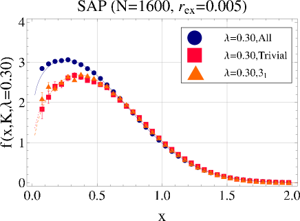
In the case of thin cylindrical SAP with radius re​x=0.005subscriptπ‘Ÿπ‘’π‘₯0.005r_{ex}=0.005 we plotted in Fig. 19 the data points of distibution functions fK​(x;Ξ»,N)subscript𝑓𝐾π‘₯πœ†π‘f_{K}(x;\lambda,N) of normalized distance xπ‘₯x between two nodes of cylindrical SAP of N=1,600𝑁1600N=1,600 with parameter Ξ»=0.3πœ†0.3\lambda=0.3. Here we recall that the two nodes of SAP are separated by λ​Nπœ†π‘\lambda N steps along the chain. We consider the three topological conditions: the trivial knot (01subscript010_{1}), the trefoil knot (31subscript313_{1}) and no toplogical constaint (A​l​l𝐴𝑙𝑙All). The fitting curves given by formula (38) are also plotted in Fig. 19, which are determined with two fitting parameters ΞΈKsubscriptπœƒπΎ\theta_{K} and Ξ΄Ksubscript𝛿𝐾\delta_{K}.

Refer to caption
Figure 19: Data points and fittung curves of the distibution functions fK​(x;Ξ»,N)subscript𝑓𝐾π‘₯πœ†π‘f_{K}(x;\lambda,N) of normalized distance xπ‘₯x between two nodes of cylindrical SAP of N=1600𝑁1600N=1600 with radius r=0.005π‘Ÿ0.005r=0.005 (thin cylinders) for topological conditions, such as the trivial knot (01subscript010_{1}), the trefoil knot (31subscript313_{1}) and no toplogical constaint (A​l​l𝐴𝑙𝑙All) (thin cylinders).

Also for the thin cylidrical SAP the Ο‡2superscriptπœ’2\chi^{2} values per datum are small for all the three topological conditions. We find that the fitting curves to the distribution functions are good. The fitting parameters are listed in Table 5.

The estimates of exponent ΞΈKsubscriptπœƒπΎ\theta_{K} in the thin case are much smaller than the case of thick SAP. For instance, we have ΞΈa​l​l=0.2subscriptπœƒπ‘Žπ‘™π‘™0.2\theta_{all}=0.2. It is maybe due to the fact that the excluded volume effect is not strong, yet. Here we recall that we have observed in Fig. 11 the excluded volume effect does not clearly appear for SAP of N=1600𝑁1600N=1600 segments in the case of re​x=0.005subscriptπ‘Ÿπ‘’π‘₯0.005r_{ex}=0.005.

K𝐾K No constraint (A​l​l𝐴𝑙𝑙All) trivial knot (00) trefoil knot (31subscript313_{1})
ΞΈKsubscriptπœƒπΎ\theta_{K} 0.161 Β±0.005plus-or-minus0.005\pm 0.005 0.26 Β±0.02plus-or-minus0.02\pm 0.02 0.33 Β±0.02plus-or-minus0.02\pm 0.02
νKsubscript𝜈𝐾\nu_{K} 0.538 ±0.001plus-or-minus0.001\pm 0.001 0.582 ±0.004plus-or-minus0.004\pm 0.004 0.551 ±0.004plus-or-minus0.004\pm 0.004
Ο‡2superscriptπœ’2\chi^{2}/datum 3.32 0.492 1.26
Table 5: Estimates of fitting parameters and the Ο‡2superscriptπœ’2\chi^{2} value per datum for the fitting curves in Fig. 19: re​x=0.005subscriptπ‘Ÿπ‘’π‘₯0.005r_{ex}=0.005, Ξ»=πœ†absent\lambda= 0.3 and N=1600𝑁1600N=1600.

4.4 Correlation functions through exponents θ​(Ξ»)πœƒπœ†\theta(\lambda)

We now discuss that the distribution function of the distance between two points of SAP with knot type K𝐾K, pK​(r;i,j;N)subscriptπ‘πΎπ‘Ÿπ‘–π‘—π‘p_{K}(r;i,j;N), is useful for constructing various important quantities of knotted ring polymers in solution. Let us assume that the two points are separated by λ​Nπœ†π‘\lambda N steps along the chain of the SAP. Due to the translational symmetry among the vertices of SAP along the chain, the expressions of the physical quantities are much simpler than those of SAW. Here we remark that the structrue factor of dilute ring polymers have been studied numerically [37].

The pair correlation function of SAP with knot K𝐾K is given by

gK​(r)subscriptπ‘”πΎπ‘Ÿ\displaystyle g_{K}(r) =\displaystyle= 1Nβ€‹βˆ‘i=1Nβˆ‘j=1NpK​(r;i,j;N)1𝑁superscriptsubscript𝑖1𝑁superscriptsubscript𝑗1𝑁subscriptπ‘πΎπ‘Ÿπ‘–π‘—π‘\displaystyle{\frac{1}{N}}\sum_{i=1}^{N}\sum_{j=1}^{N}p_{K}(r;i,j;N) (40)
=\displaystyle= βˆ‘j=1NpK​(r;0,j;N).superscriptsubscript𝑗1𝑁subscriptπ‘πΎπ‘Ÿ0𝑗𝑁\displaystyle\sum_{j=1}^{N}p_{K}(r;0,j;N)\,.

In terms of parameter Ξ»πœ†\lambda we express it as a single integral as follows.

gK​(r)=Nβ€‹βˆ«01𝑑λ​pK​(r;Ξ»;N).subscriptπ‘”πΎπ‘Ÿπ‘superscriptsubscript01differential-dπœ†subscriptπ‘πΎπ‘Ÿπœ†π‘g_{K}(r)=N\int_{0}^{1}d\lambda\,p_{K}(r;\lambda;N)\,. (41)

5 Diffusion constants of knotted SAP

We now evaluate the diffusion coefficient of N𝑁N-noded cylindrical SAP with a knot type K𝐾K in solution by Kirkwood’s approximation.

DG,K=kB​T6​π​ηs​N2β€‹βˆ‘i=1Nβˆ‘j=1N⟨1|𝑹iβˆ’π‘Ήj|⟩K.subscript𝐷𝐺𝐾subscriptπ‘˜π΅π‘‡6πœ‹subscriptπœ‚π‘ superscript𝑁2superscriptsubscript𝑖1𝑁superscriptsubscript𝑗1𝑁subscriptdelimited-⟨⟩1subscript𝑹𝑖subscript𝑹𝑗𝐾D_{G,K}={\frac{k_{B}T}{6\pi\eta_{s}N^{2}}}\sum_{i=1}^{N}\sum_{j=1}^{N}\langle\frac{1}{|{\mbox{\boldmath$R$}}_{i}-{\mbox{\boldmath$R$}}_{j}|}\rangle_{K}\,. (42)

Here we recall that Ξ·ssubscriptπœ‚π‘ \eta_{s} denotes the solvent viscosity and βŸ¨β‹…βŸ©Ksubscriptdelimited-βŸ¨βŸ©β‹…πΎ\langle\cdot\rangle_{K} denotes the average over all configurations of SAP with a given knot type K𝐾K.

The estimates of the diffusion coefficient DG,Ksubscript𝐷𝐺𝐾D_{G,K} of cylindrical SAP with radius re​x=0.1subscriptπ‘Ÿπ‘’π‘₯0.1r_{ex}=0.1 are plotted against the number N𝑁N of nodes for no topological constraint denoted 01subscript010_{1} and the trivial knot denote 01subscript010_{1} in Fig. 20 in double-logarithmic scales. Here, we evaluated the ensemble average ⟨1|𝑹iβˆ’π‘Ήj|⟩Ksubscriptdelimited-⟨⟩1subscript𝑹𝑖subscript𝑹𝑗𝐾\langle\frac{1}{|{\mbox{\boldmath$R$}}_{i}-{\mbox{\boldmath$R$}}_{j}|}\rangle_{K} by taking the sum over all the configurations of SAP with knot type K𝐾K.

For the two topological conditions, K=A​l​l𝐾𝐴𝑙𝑙K=All and K=01𝐾subscript01K=0_{1}, the diffusion coeffiicents coincide with each other. Furthermore, they are well fitted by a staright line in the double-logarithmic scale. For the thick cylinder case, the topology of the majority of SAPs is given by the trivial knot, and hence DG,A​l​lsubscript𝐷𝐺𝐴𝑙𝑙D_{G,All} and DG,01subscript𝐷𝐺subscript01D_{G,0_{1}} have the same value.

Refer to caption
Figure 20: Double logarithmic plot of diffusion coefficient of N𝑁N noded cylindrical SAP under topological condition K𝐾K. The SAP consists of N𝑁N thick cylindrical segments with radius rex=0.1subscriptπ‘Ÿex0.1r_{\rm ex}=0.1 of unit length. Filled blue circle and filled red diamonds denote no topological constraint (A​l​l𝐴𝑙𝑙All) and the trivial knot (01subscript010_{1}), respectively. The sum 1N2β€‹βˆ‘i=1Nβˆ‘j=1N⟨1|𝑹iβˆ’π‘Ήj|⟩K1superscript𝑁2superscriptsubscript𝑖1𝑁superscriptsubscript𝑗1𝑁subscriptdelimited-⟨⟩1subscript𝑹𝑖subscript𝑹𝑗𝐾{\frac{1}{N^{2}}}\sum_{i=1}^{N}\sum_{j=1}^{N}\langle\frac{1}{|{\mbox{\boldmath$R$}}_{i}-{\mbox{\boldmath$R$}}_{j}|}\rangle_{K} is plotted.
Refer to caption
Figure 21: Ratio of diffusion coefficients, DG,K/DG,01subscript𝐷𝐺𝐾subscript𝐷𝐺subscript01D_{G,K}/D_{G,0_{1}}, is plotted against the number of nodes N𝑁N. Here DG,Ksubscript𝐷𝐺𝐾D_{G,K} denotes the diffusion coefficient of N𝑁N-noded cylindrical SAP with rex=0.10subscriptπ‘Ÿex0.10r_{\rm ex}=0.10 for given topological condition K𝐾K, and 01subscript010_{1} denotes the trivial knot.

The ratio of diffusion coefficients DG,K/DG,01subscript𝐷𝐺𝐾subscript𝐷𝐺subscript01D_{G,K}/D_{G,0_{1}} is plotted against the number of segments N𝑁N in Fig. 21. Here we recall that the diffusion coefficient of SAP under no topological constraint and that of the trivial knot coincides numerically very well.

We observe in Fig. 21 that the ratio gradually decreases with respect to the number of N𝑁N. We suggest that it reaches an asymptotically constant value at some large value of N𝑁N. Following renormalization group arguments we expect that the ratio should be universal and independent of details of models. It would be interesting to compare the ratio with experimental data in future.

The diffusion coeffiecient of the figure-eight knot has large error bars due to the number of SAP with the knot type is very small for the thick case with cylindrical radius re​x=0.1subscriptπ‘Ÿπ‘’π‘₯0.1r_{ex}=0.1.

In the method of Kirkwood’s approximation we can express diffusion coefficient DG,Ksubscript𝐷𝐺𝐾D_{G,K} in terms of the probability distribution functions of the distance between two nodes of SAP. Here we take the sum over all pairs i𝑖i and j𝑗j of SAP as follows.

DG,Ksubscript𝐷𝐺𝐾\displaystyle D_{G,K} =\displaystyle= kB​T6​π​ηs​N2β€‹βˆ‘i=1Nβˆ‘j=1N∫0∞1r​pK​(r;i,j;N)​ 4​π​r2.subscriptπ‘˜π΅π‘‡6πœ‹subscriptπœ‚π‘ superscript𝑁2superscriptsubscript𝑖1𝑁superscriptsubscript𝑗1𝑁superscriptsubscript01π‘Ÿsubscriptπ‘πΎπ‘Ÿπ‘–π‘—π‘4πœ‹superscriptπ‘Ÿ2\displaystyle{\frac{k_{B}T}{6\pi\eta_{s}N^{2}}}\sum_{i=1}^{N}\sum_{j=1}^{N}\int_{0}^{\infty}\,{\frac{1}{r}}\,p_{K}(r;i,j;N)\,4\pi r^{2}. (43)

Considering the cyclic symmetry of SAP we reduce the double sum into the single sum, as follows.

βˆ‘i=1Nβˆ‘j=1N∫0∞1r​pK​(r;i,j;N)​ 4​π​r2=Nβ€‹βˆ‘j=1N∫0∞1r​pK​(r;0,j;N)​ 4​π​r2.superscriptsubscript𝑖1𝑁superscriptsubscript𝑗1𝑁superscriptsubscript01π‘Ÿsubscriptπ‘πΎπ‘Ÿπ‘–π‘—π‘4πœ‹superscriptπ‘Ÿ2𝑁superscriptsubscript𝑗1𝑁superscriptsubscript01π‘Ÿsubscriptπ‘πΎπ‘Ÿ0𝑗𝑁4πœ‹superscriptπ‘Ÿ2\sum_{i=1}^{N}\sum_{j=1}^{N}\int_{0}^{\infty}\,{\frac{1}{r}}\,p_{K}(r;i,j;N)\,4\pi r^{2}=N\sum_{j=1}^{N}\int_{0}^{\infty}\,{\frac{1}{r}}\,p_{K}(r;0,j;N)\,4\pi r^{2}\,. (44)

In terms of Ξ»πœ†\lambda we have the following expression.

DG,K=kB​T6​π​ηsβ€‹βˆ«01π‘‘Ξ»β€‹βˆ«0∞1r​pK​(r;Ξ»;N)​ 4​π​r2.subscript𝐷𝐺𝐾subscriptπ‘˜π΅π‘‡6πœ‹subscriptπœ‚π‘ superscriptsubscript01differential-dπœ†superscriptsubscript01π‘Ÿsubscriptπ‘πΎπ‘Ÿπœ†π‘4πœ‹superscriptπ‘Ÿ2D_{G,K}={\frac{k_{B}T}{6\pi\eta_{s}}}\int_{0}^{1}d\lambda\,\int_{0}^{\infty}\,{\frac{1}{r}}\,p_{K}(r;\lambda;N)\,4\pi r^{2}\,. (45)

6 Concluding remarks

We have shown that formula (16) gives good fitting curves to the data of the probability distribution functions of the distance between two points of SAW, f0​(x;N)subscript𝑓0π‘₯𝑁f_{0}(x;N) and fs​(x;Ξ»,N)subscript𝑓𝑠π‘₯πœ†π‘f_{s}(x;\lambda,N) for s=1,2𝑠12s=1,2, over a wide range of the normalized distance xπ‘₯x such as from x=0.05π‘₯0.05x=0.05 to 1.95.

In the case of large xπ‘₯x, the distribution functions have the same asymptotic behavior: fs​(x;Ξ»,N)∝exp⁑(βˆ’xΞ΄)proportional-tosubscript𝑓𝑠π‘₯πœ†π‘superscriptπ‘₯𝛿f_{s}(x;\lambda,N)\propto\exp(-x^{\delta}) with Ξ΄=1/(1βˆ’Ξ½)𝛿11𝜈\delta=1/(1-\nu) for many different values of Ξ»πœ†\lambda such as from Ξ»πœ†\lambda = 0.10 to 0.98. Thus, exponent δ𝛿\delta does not change for s=0,1,2𝑠012s=0,1,2 and for various values of Ξ»πœ†\lambda. Moreover, exponent δ𝛿\delta does not change for any vertices i𝑖i and j𝑗j of N𝑁N-step SAW.

We evaluated the exponents ΞΈssubscriptπœƒπ‘ \theta_{s} which describe and characterize the short-distance behaviour of fs​(x;Ξ»,N)subscript𝑓𝑠π‘₯πœ†π‘f_{s}(x;\lambda,N), from the fitting curves to the data points from x=0.05π‘₯0.05x=0.05 to 1.95, which is almost the entire region of xπ‘₯x. The estimates of ΞΈ1​(Ξ»)subscriptπœƒ1πœ†\theta_{1}(\lambda) are clealry smaller than the theoretical value ΞΈ1(R​G)=0.46superscriptsubscriptπœƒ1𝑅𝐺0.46\theta_{1}^{(RG)}=0.46 for 0.1<Ξ»<0.80.1πœ†0.80.1<\lambda<0.8; The estimates of ΞΈ2​(Ξ»)subscriptπœƒ2πœ†\theta_{2}(\lambda) are approximately equal to the theoretical value ΞΈ2(R​G)=0.71superscriptsubscriptπœƒ2𝑅𝐺0.71\theta_{2}^{(RG)}=0.71 for 0.1<Ξ»<0.50.1πœ†0.50.1<\lambda<0.5.

We evaluated exponents θ​(i,j)πœƒπ‘–π‘—\theta(i,j) which describe the short-distance interchain correlation between vertices i𝑖i and j𝑗j of N𝑁N-step SAW. They generalize des Cloizeaux’s three exponents ΞΈssubscriptπœƒπ‘ \theta_{s} for s=0,1,2𝑠012s=0,1,2. Expressing vertices i𝑖i and j𝑗j in terms of parameters Ξ»πœ†\lambda and ΞΌπœ‡\mu we observed the crossover of exponents θ​(i,j)πœƒπ‘–π‘—\theta(i,j): from ΞΈ2subscriptπœƒ2\theta_{2} to ΞΈ1subscriptπœƒ1\theta_{1} and from ΞΈ1subscriptπœƒ1\theta_{1} to ΞΈ0subscriptπœƒ0\theta_{0} as Ξ»πœ†\lambda approaches 1; exponent θ​(i,j)πœƒπ‘–π‘—\theta(i,j) changes from ΞΈ2subscriptπœƒ2\theta_{2} to ΞΈ1subscriptπœƒ1\theta_{1} as parameter ΞΌπœ‡\mu approaches 0.

We have shown that formula (38) gives good fitting curves to the data of the probability distribution functions of the distance between two points of cylindrical SAP. For the thick cylinder case of cylindrical radius re​x=0.1subscriptπ‘Ÿπ‘’π‘₯0.1r_{ex}=0.1 the estimates of exponent θ​(Ξ»)πœƒπœ†\theta(\lambda) for the short-distance correlation is a little smaller than the theoretical value ΞΈ2(R​G)superscriptsubscriptπœƒ2𝑅𝐺\theta_{2}^{(RG)} of SAW.

Finally, we suggest that the results of this paper should be useful for studying the scaling behaviour of interchain correlation for toplogical polymers with more complex structures.

Acknowledgement

The authors would like to thank B. Duplantier for bringing us Ref. [29]. They are grateful to Dr. A. Yao for helpful comments.


References

  • [1] M.A. Krasnow, A. Stasiak, S.J. Spengler, F. Dean, T. Koller and N.R. Cozzarelli, Nature, 304, 559 (1983).
  • [2] F.B. Dean, A. Stasiak, T. Koller and N.R. Cozzarelli, J. Biol. Chem., 260, 4975 (1985).
  • [3] A.D.Β Bates and A.Β Maxwell, DNA Topology (Oxford Univ. Press, 2005)
  • [4] D. J. Craik, Science 311, 1563 (2006).
  • [5] C. W. Bielawski, D. Benitez and R. H. Grubbs, Science 297, 2041–2044 (2002).
  • [6] D. Cho, K. Masuoka, K. Koguchi, T. Asari, D. Kawaguchi, A. Takano and Y. Matsushita, Polymer Journal 37, 506–511 (2005).
  • [7] A. Takano, Y. Kushida, K. Aoki, K. Masuoka, K. Hayashida, D. Cho, D. Kawaguchi and Y. Matsushita, Macromolecules 40, 679–681 (2007).
  • [8] B. A. Laurent and S. Grayson, J. Am. Chem. Soc. 128, 4238–4239 (2006).
  • [9] N. Sugai, H. Heguri, K. Ohta, Q. Meng, T. Yamamoto and Y. Tezuka, J. Am. Chem. Soc. 132, 14790–14802 (2010)
  • [10] N. Sugai, H. Heguri, T. Yamamoto and Y. Tezuka, JACS 133, 19694–19697 (2011).
  • [11] Topological Polymer Chamistry: Progress in cyclic polymers in syntheses, properties and functions, ed. by Y. Tezuka, (World Scientific Publ., Singapore, 2013).
  • [12] E. Orlandini and S. G. Whittington, Rev. Mod. Phys., 79, 611 (2007).
  • [13] C. Micheletti, D. Marenduzzo and E. Orlandini, Phys. Rep., 504, 1 (2011).
  • [14] β€œStatistical physics and topology of polymers with ramifications to structure and function of DNA and proteins”, eds. T. Deguchi et al., Prog. Theor. Phys. Suppl., 191, (2011).
  • [15] J.Β M. Deutsch, Phys. Rev. E, 59, R2539 (1999).
  • [16] A.Β Yu. Grosberg, Phys. Rev. Lett., 85, 3858 (2000).
  • [17] M.Β K.Β Shimamura and T. Deguchi, Phys. Rev. E, 65, 051802 (2002).
  • [18] M. K.Β  Shimamura and T.Β Deguchi, J. Phys. A: Math. Gen., 35, L241 (2002).
  • [19] A. Dobay, J. Dubochet, K. Millett, P.Β E. Sottas and A. Stasiak, Proc. Natl. Acad. Sci. USA, 100, 5611 (2003).
  • [20] H. Matsuda, A. Yao, H. Tsukahara, T. Deguchi, K. Furuta and T. Inami, Phys. Rev. E, 68, 011102 (2003).
  • [21] N.Β T. Moore, R.Β C. Lua and A.Β Y. Grosberg, Proc. Natl. Acad. Sci. USA, 101, 13431 (2004).
  • [22] A. Takano, Y. Ohta, K. Masuoka, K. Matsubara, T. Nakano, A. Hieno, M. Itakura,K. Takahashi, S. Kinugasa, D. Kawaguchi, Y. Takahashi, and Y. Matsushita, Macromolecules, 45, 369 (2012).
  • [23] P.G. de Gennes, Scaling Concepts in Polymer Physics (Cornell Univ. Press, Ithaka and New York, 1979).
  • [24] M. Doi and S.F. Edwards, The Theory of Polymer Dynamics, (Oxford University Press, Oxford, 1986).
  • [25] R. Guida and J. Zinn-Justin, J. Phys. A: Math. Gen. 31, 8103 (1988)
  • [26] M. E. Fisher, J. Chem. Phys. 44, 616 (1966).
  • [27] D.S. McKenzie and M.A. Moore, J. Phys. A 4, L82 (1971).
  • [28] J. des Cloizeaux, Phys. Rev. A 10, 1665 (1974).
  • [29] J. des Cloizeaux, J. Physique 41, 223 (1980).
  • [30] A. BaumgΓ€rtner, Z. Phys. B, Cond. Mat. 42, 265 (1981).
  • [31] Y. Oono and T. Ohta, Phys. Lett. A 85, 480 (1981).
  • [32] B. Duplantier, J. Physique 47, 1633 (1981).
  • [33] B. Duplantier, J. Physique Lett. 46, 751 (1985).
  • [34] M. Bishop and H.R. clarke, J. Chem. Phys. 94, 3936 (1991); J. Chem. Phys. 95, 4589 (1991).
  • [35] J.P. Valleau, J. Chem. Phys. 116, 3071 (1996).
  • [36] E.G. Timoshenko, Y.A. Kuznetsov and R. Connolly, J. Chem. Phys. 116, 3905 (2002).
  • [37] P. Calabrese, A. Pelissetto and E. Vicari, J. Chem. Phys. 116, 8191 (2002).
  • [38] J. des Cloizeaux, J. Phys. Let. (France), 42 , L433 (1981).
  • [39] A.Β Yao, H.Β Tsukahara, T.Β Deguchi and T.Β Inami, J. Phys. A: Math. Gen., 37, 7993 (2004).
  • [40] M.Β K.Β Shimamura, K.Β Kamata, A.Β Yao and T.Β Deguchi, Phys. Rev. E, 72, 041804 (2005).
  • [41] T. Deguchi and A. Yao, OCAMI Studies 1, 165 (2007).
  • [42] Y. Akita, Master Thesis, Ochanomizu University, March, 2010 (in Japanese).
  • [43] J. Suzuki, A. Takano and Y. Matsushita, J. Chem. Phys. 138, 024902 (2013).
  • [44] N. Madras and A.D. Sokal, J. Stat. Phys. 50, 109 (1988).
  • [45] N. Madras, A. Orlitsky and L.A. Shepp, J. Stat. Phys. 58, 159 (1990).