Enhanced violation of a Leggett-Garg inequality under nonequilibrium thermal conditions

Juan C. Castillo Departamento de Física, Universidad de los Andes, A.A. 4976 Bogotá, D.C.,Colombia    Ferney J. Rodríguez Departamento de Física, Universidad de los Andes, A.A. 4976 Bogotá, D.C.,Colombia    Luis Quiroga Departamento de Física, Universidad de los Andes, A.A. 4976 Bogotá, D.C.,Colombia
Abstract

We investigate both analytically and numerically violations of a Leggett-Garg inequality (LGI) for a composite quantum system in contact with two separate reservoirs at different temperatures. Remarkably we find that LGI violations can be enhanced when a heat current is established at low temperatures in a steady-state regime. Based on a Kraus operator decomposition of the non-unitary evolution for a system formed by two interacting spins or quantum bits, we provide analytical support for power law relations between dissipation strength and mean temperature in the borderlines separating parameter regions where non-equilibrium conditions affect differently the maximal LGI violation. Furthermore, a correspondence between spatial and temporal correlation inequalities is shown to persist even in such nonequilibrium thermal settings.

pacs:
03.67.Mn, 03.65.Ud, 65.40.Gr

I Introduction

Since the seminal work by John Bell  bell about quantum spatial correlations, an ever increasing number of experiments has been devoted to test the foundations of quantum mechanics. In a parallel way, and triggered by those tests, practical schemes for conveying quantum information have flourished. New aspects of the fascinating world of quantum correlations arose when temporal, instead of spatial, correlations were proposed by Leggett and Garg leggett , and subsequently by many other authors paz ; huelga ; kofler . In those works different inequalities between two-time correlations have been proposed that should hold whenever a classical description is valid. An emerging Leggett-Garg inequality (LGI) violation would mark a borderline between the classical and quantum worlds. Of special interest has been the guide provided by LGI for testing macroscopic realism in condensed matter systems nori ; palacios ; goggin ; knee ; jordan ; athalye ; waldherr as well as in quantum optics setups xu ; dressel where focus has been put on LGI violations for open quantum systems in contact with realistic reservoirs.

On the other hand, one of the most important challenges to detect superposition of quantum macroscopic states is the fragility of these states caused by decoherence effects. Despite the ubiquitous presence of non-equilibrium situations in quantum mesoscopic and macroscopic physics, few formal results about quantum correlations in such regimes are available quiroga ; polko ; cazalilla ; plenio . Many efforts encompassing a large variety of physical systems have been directed to study the effects of spatial correlations, as measured by the concurrence brandes ; quiroga ; petruccione1 and quantum discord (QD) wu1 , under non-equilibrium gradients. However, LGI studies have been very scarce in systems out of thermodynamic equilibrium, although time correlations in condensed matter systems show complex and interesting behaviors, like those observed in ultracold atom systems greiner , inductively (capacitively) coupled flux (charge) superconducting qubits simmonds , and even energy transfer processes in photosynthetic purple bacteria sarovar .

How do thermal non-equilibrium conditions affect quantum two-time correlations? From a theoretical point of view important insights have been given in Ref.scully where nanothermodynamics relevance of quantum coherences has been addressed. From the experimental side Ref.giazotto shows an elegant experiment where thermal and electric currents interfere in a Josephson junction. Here, we propose a set up where the relationship between two-time quantum correlations and out-of-equilibrium thermal conditions can be systematically explored through the LGI violations. Here, we examine a LGI for a two-qubit system and show that violations are enhanced when a heat current, 𝒥𝒥{\cal J}, is flowing through it.

For nonequilibrium dynamics, what is the optimal relationship between dissipation strength (ΓΓ\Gamma) and temperature range (T𝑇T) which allows the detection of quantum correlations through macroscopic transport measurements? The theoretical approach we provide, in terms of Kraus operator dynamics evolution, gives a general framework to identify non-classical features through LGI violations for quantum systems in contact with two memoryless (Markovian) separate reservoirs at different temperatures. We find that dissipation, inter-qubit interactions and mean temperature compete, resulting in a rich T𝑇T-ΓΓ\Gamma phase diagram where power-law relations mark the boundaries between different zones where LGI violations are either absent, decreasing or increasing with an applied temperature gradient.

The structure of the paper is as follows. In Sec II we give the details about the Leggett-Garg inequalities in a generic non-thermal steady state and the calculation of two-time quantum correlations. In Sec. III we describe our model of two interconnected qubits each one interacting with an independent thermal bath. The nonequilibrium situation arises when the two baths are at different temperatures. In Sec. IV, we present our main analytical and numerical results about the nonequilibrium enhanced LGI violation. Our main conclusions are summarized in Sec. V while technical details are described in the Appendixes.

II Legget-Garg inequalities in a nonequilibrium steady-state

The two-time correlation inequality, LGI, extends the well-known Bell inequality (designed to probe spatial quantum correlations) to the time domain. One form the LGI can take is leggett ; paz ; huelga ; avis :

F(t1,t2,t3)=C(t1,t2)+C(t2,t3)C(t1,t3)1𝐹subscript𝑡1subscript𝑡2subscript𝑡3𝐶subscript𝑡1subscript𝑡2𝐶subscript𝑡2subscript𝑡3𝐶subscript𝑡1subscript𝑡31\displaystyle F(t_{1},t_{2},t_{3})=C(t_{1},t_{2})+C(t_{2},t_{3})-C(t_{1},t_{3})\leq 1 (1)

where C(ti,tj)𝐶subscript𝑡𝑖subscript𝑡𝑗C(t_{i},t_{j}) is the two-time correlation of a dichotomic observable Q^^𝑄\hat{Q} (eigenvalues a𝑎a=±1plus-or-minus1\pm 1) between times tisubscript𝑡𝑖t_{i} and tjsubscript𝑡𝑗t_{j} and t1<t2<t3subscript𝑡1subscript𝑡2subscript𝑡3t_{1}<t_{2}<t_{3}. To evaluate F(t1,t2,t3)𝐹subscript𝑡1subscript𝑡2subscript𝑡3F(t_{1},t_{2},t_{3}) in Eq.(1), a Kraus operator K^(t)^𝐾𝑡\hat{K}(t) approach has been used krauss . For the sake of completeness, here we briefly review the Kraus operator formalism and show how it applies to a nonequilibrium steady-state regime.

II.1 Kraus operators

Consider a physical system with quantum states in a Hilbert space \mathcal{H}. The time evolution of its density matrix ρ(t)𝜌𝑡\rho(t) is described by the following Lindblad equation:

tρ(t)=[ρ(t)]=i[H,ρ(t)]+𝒟[ρ(t)]𝑡𝜌𝑡delimited-[]𝜌𝑡𝑖𝐻𝜌𝑡𝒟delimited-[]𝜌𝑡\frac{\partial}{\partial t}\rho(t)=\mathcal{L}\left[\rho(t)\right]=-i\left[H,\rho(t)\right]+\mathcal{D}\left[\rho(t)\right] (2)

with a time-independent Lindbladian superoperator \mathcal{L}, where 𝒟𝒟\mathcal{D} is the dissipator or nonunitary evolution term. The goal is to find a form for the evolution superoperator (t1t2)subscript𝑡1subscript𝑡2\mathcal{E}(t_{1}-t_{2}), which maps an initial density operator of the system to a final density operator, as defined by

ρ(t2)=(t1t2)[ρ(t1)]𝜌subscript𝑡2subscript𝑡1subscript𝑡2delimited-[]𝜌subscript𝑡1\rho(t_{2})=\mathcal{E}(t_{1}-t_{2})\left[\rho(t_{1})\right] (3)

This form generates a semigroup associated with a Markovian dynamics. Thus, the evolution only depends on the time interval between t1subscript𝑡1t_{1} and t2subscript𝑡2t_{2}. An elegant and efficient form of expressing (t1t2)subscript𝑡1subscript𝑡2\mathcal{E}(t_{1}-t_{2}) is using the Kraus operators via the following equation:

ρ(t+t)=(t)[ρ(t)]=μKμ(t)ρ(t)Kμ(t)𝜌superscript𝑡𝑡𝑡delimited-[]𝜌superscript𝑡subscript𝜇subscript𝐾𝜇𝑡𝜌superscript𝑡superscriptsubscript𝐾𝜇𝑡\rho(t^{\prime}+t)=\mathcal{E}(t)\left[\rho(t^{\prime})\right]=\sum_{\mu}K_{\mu}(t)\rho(t^{\prime})K_{\mu}^{\dagger}(t) (4)

where the Kraus operators Kμsubscript𝐾𝜇K_{\mu} fulfill the condition μKμ(t)Kμ(t)=1subscript𝜇superscriptsubscript𝐾𝜇𝑡subscript𝐾𝜇𝑡1\sum_{\mu}K_{\mu}^{\dagger}(t)K_{\mu}(t)=1 in order to preserve the unit trace of the density operator at any time. It can easily be shown that, replacing the Kraus operators with unitary evolution operators, the exact results for closed quantum systems are retrieved. Since the Kraus representation describes equivalently the nonunitary time evolution of an open quantum system we can conclude that the Kraus operators depend only on the time interval and give direct access to time correlation functions of the open system. However, the explicit calculation of Kraus operators can be a complex task beyond simple, and generally, non-interacting composite quantum systems. As discussed below we find them in a numerical way for an interacting spin chain out-of-equilibrium.

II.2 Two-time quantum correlations in terms of Kraus operators

The time correlations C(ti,tj)𝐶subscript𝑡𝑖subscript𝑡𝑗C(t_{i},t_{j}) in Eq.(1) are evaluated as leggett ; kofler

C(ti,tj)𝐶subscript𝑡𝑖subscript𝑡𝑗\displaystyle C(t_{i},t_{j}) =\displaystyle= p(+ti)q(+tj|+ti)+p(ti)q(tj|ti)\displaystyle p(^{+}t_{i})q(^{+}t_{j}|^{+}t_{i})+p(^{-}t_{i})q(^{-}t_{j}|^{-}t_{i}) (5)
\displaystyle- p(ti)q(+tj|ti)p(+ti)q(tj|+ti)\displaystyle p(^{-}t_{i})q(^{+}t_{j}|^{-}t_{i})-p(^{+}t_{i})q(^{-}t_{j}|^{+}t_{i})

where p(ati)p(^{a}t_{i}) is the probability of obtaining the result a=±1𝑎plus-or-minus1a=\pm 1 at tisubscript𝑡𝑖t_{i}, and q(ati|btl)q(^{a}t_{i}|^{b}t_{l}) is the conditional probability of getting the result a=±1𝑎plus-or-minus1a=\pm 1 at tisubscript𝑡𝑖t_{i} given that result b=±1𝑏plus-or-minus1b=\pm 1 was obtained at tlsubscript𝑡𝑙t_{l}.

Now, we show the connection between Kraus operators and conditional/unconditional probabilities involved in obtaining two-time quantum correlations in Eq.(5). To find each one of these probabilities, we must use the projector Π^±superscript^Πplus-or-minus\hat{\Pi}^{\pm}, related to the eigenspaces of the observable Q^^𝑄\hat{Q}, in terms of which p(ati)=Tr{Π^aρ^(ti)}p(^{a}t_{i})=\mathrm{Tr}\left\{\hat{\Pi}^{a}\hat{\rho}(t_{i})\right\}. To proceed further, the conditional probabilities q(ati|btl)q(^{a}t_{i}|^{b}t_{l}) should be obtained. A generic term in the right hand side of Eq.(5) becomes

p(ati)q(ati|btl)\displaystyle p(^{a}t_{i})q(^{a}t_{i}|^{b}t_{l}) =\displaystyle= Tr{Π^aν,μK^ν(titl)Π^bK^μ(tl)ρ^0\displaystyle\mathrm{Tr}\left\{\hat{\Pi}^{a}\sum_{\nu,\mu}\hat{K}_{\nu}(t_{i}-t_{l})\hat{\Pi}^{b}\hat{K}_{\mu}(t_{l})\hat{\rho}_{0}\right. (6)
K^μ(tl)Π^bK^ν(titl)}\displaystyle\left.\hat{K}^{\dagger}_{\mu}(t_{l})\hat{\Pi}^{b}\hat{K}^{\dagger}_{\nu}(t_{i}-t_{l})\right\}

The expression for p(jti)p(^{j}t_{i}) (with j=±𝑗plus-or-minusj=\pm) is now

p(jti)=Tr{Πjρ(ti)}=Tr{ΠjμKμ(ti)ρ0Kμ(ti)}\displaystyle p(^{j}t_{i})=\mathrm{Tr}\left\{\Pi^{j}\rho(t_{i})\right\}=\mathrm{Tr}\left\{\Pi^{j}\sum_{\mu}K_{\mu}(t_{i})\rho_{0}K^{\dagger}_{\mu}(t_{i})\right\} (7)

To obtain an expression for q(jti|ktl)q(^{j}t_{i}|^{k}t_{l}) (where j,k=±𝑗𝑘plus-or-minusj,k=\pm), we must also find the density matrix corresponding to a measurement result k𝑘k obtained at time tlsubscript𝑡𝑙t_{l}:

ρk(tl)=Πkρ(tl)ΠkTr{Πkρ(tl)}=ΠkμKμ(tl)ρ0Kμ(tl)Πkp(jtl)\rho^{k}(t_{l})=\frac{\Pi^{k}\rho(t_{l})\Pi^{k}}{\mathrm{Tr}\left\{\Pi^{k}\rho(t_{l})\right\}}=\frac{\Pi^{k}\sum_{\mu}K_{\mu}(t_{l})\rho_{0}K^{\dagger}_{\mu}(t_{l})\Pi^{k}}{p(^{j}t_{l})} (8)

This state now evolves until tisubscript𝑡𝑖t_{i}, when the state of the system is νKν(titl)ρk(tl)Kν(titl)subscript𝜈subscript𝐾𝜈subscript𝑡𝑖subscript𝑡𝑙superscript𝜌𝑘subscript𝑡𝑙subscriptsuperscript𝐾𝜈subscript𝑡𝑖subscript𝑡𝑙\sum_{\nu}K_{\nu}(t_{i}-t_{l})\rho^{k}(t_{l})K^{\dagger}_{\nu}(t_{i}-t_{l}), so that

q(jti|ktl)=Tr{ΠjνμKν(titl)ΠkKμ(tl)ρ0Kμ(tl)ΠkKν(titl)}p(jti)q(^{j}t_{i}|^{k}t_{l})=\frac{\mathrm{Tr}\left\{\Pi^{j}\sum_{\nu\mu}K_{\nu}(t_{i}-t_{l})\Pi^{k}K_{\mu}(t_{l})\rho_{0}K^{\dagger}_{\mu}(t_{l})\Pi^{k}K^{\dagger}_{\nu}(t_{i}-t_{l})\right\}}{p(^{j}t_{i})} (9)

With all these ingredients the two-time quantum correlations can finally be written as (see Appendix A for details):

C(t1,t2)=12p(+t1)2p(+t2)+4Re[g(t1,t2)]\displaystyle C(t_{1},t_{2})=1-2p(^{+}t_{1})-2p(^{+}t_{2})+4\mathrm{Re}\left[g(t_{1},t_{2})\right] (10)

This expression depends mainly of the correlation function,

g(tl,ti)=Tr{Π+νKν(titl)Π+ρ(tl)Kν(titl)}𝑔subscript𝑡𝑙subscript𝑡𝑖TrsuperscriptΠsubscript𝜈subscript𝐾𝜈subscript𝑡𝑖subscript𝑡𝑙superscriptΠ𝜌subscript𝑡𝑙subscriptsuperscript𝐾𝜈subscript𝑡𝑖subscript𝑡𝑙\displaystyle g(t_{l},t_{i})=\mathrm{Tr}\left\{\Pi^{+}\sum_{\nu}K_{\nu}(t_{i}-t_{l})\Pi^{+}\rho(t_{l})K^{\dagger}_{\nu}(t_{i}-t_{l})\right\} (11)

Based on the correlations C(ti,tj)𝐶subscript𝑡𝑖subscript𝑡𝑗C(t_{i},t_{j}), the LGI function F(t1,t2,t3)𝐹subscript𝑡1subscript𝑡2subscript𝑡3F(t_{1},t_{2},t_{3}) can be written as

F(t1,t2,t3)=C(t1,t2)+C(t2,t3)C(t1,t3)1𝐹subscript𝑡1subscript𝑡2subscript𝑡3𝐶subscript𝑡1subscript𝑡2𝐶subscript𝑡2subscript𝑡3𝐶subscript𝑡1subscript𝑡31\displaystyle F(t_{1},t_{2},t_{3})=C(t_{1},t_{2})+C(t_{2},t_{3})-C(t_{1},t_{3})\leq 1 (12)
F(t1,t2,t3)=14p(+t2)+4Re[g(t1,t2)+g(t2,t3)g(t1,t3)]1\displaystyle F(t_{1},t_{2},t_{3})=1-4p(^{+}t_{2})+4Re\left[g(t_{1},t_{2})+g(t_{2},t_{3})-g(t_{1},t_{3})\right]\leq 1 (13)

This last equation, jointly with Eq.(11), is our main result allowing us to explore LGI violations in nonequilibrium set ups. From now on, we limit ourselves to consider a long-time limit or a steady-state situation where the density operator will be denoted as ρ^ss=ρ^(t)subscript^𝜌𝑠𝑠^𝜌𝑡\hat{\rho}_{ss}=\hat{\rho}(t\rightarrow\infty) which fulfills

ρ˙ss=ρss=0subscript˙𝜌𝑠𝑠subscript𝜌𝑠𝑠0\dot{\rho}_{ss}=\mathcal{L}\rho_{ss}=0 (14)

or equivalently

[t](ρss)=μKμ(t)ρssKμ(t)=ρsstformulae-sequencedelimited-[]𝑡subscript𝜌𝑠𝑠subscript𝜇subscript𝐾𝜇𝑡subscript𝜌𝑠𝑠subscriptsuperscript𝐾𝜇𝑡subscript𝜌𝑠𝑠for-all𝑡\mathcal{E}\left[t\right](\rho_{ss})=\sum_{\mu}K_{\mu}(t)\rho_{ss}K^{\dagger}_{\mu}(t)=\rho_{ss}\quad\forall t (15)

Due to this stationary state assumption, two-time correlations depend only on the time difference between two instants, which implies the non-invasive measurement requirement in LGI settings huelga .

In the calculation of the LGI function, F(t1,t2,t3)𝐹subscript𝑡1subscript𝑡2subscript𝑡3F(t_{1},t_{2},t_{3}), all three times t1subscript𝑡1t_{1}, t2subscript𝑡2t_{2} and t3subscript𝑡3t_{3} are taken in the steady-state regime and we fix them as t1=0subscript𝑡10t_{1}=0, t2=τsubscript𝑡2𝜏t_{2}=\tau and t3=2τsubscript𝑡32𝜏t_{3}=2\tau. Let us now find a simplified expression for the LGI function when the system is in the steady-state. The first step is to find an expression for p(jti)p(^{j}t_{i}) by using Eq.(7):

p(jti)=Tr{ΠjμKμ(ti)ρssKμ(ti)}=Tr{Πjρss}p(^{j}t_{i})=\mathrm{Tr}\left\{\Pi^{j}\sum_{\mu}K_{\mu}(t_{i})\rho_{ss}K^{\dagger}_{\mu}(t_{i})\right\}=\mathrm{Tr}\left\{\Pi^{j}\rho_{ss}\right\} (16)

We can thus see that it is time independent, and therefore we will simply call it pjsuperscript𝑝𝑗p^{j}. We must also find an expression for g(tl,ti)𝑔subscript𝑡𝑙subscript𝑡𝑖g(t_{l},t_{i}) from Eq.(11):

g(tl,ti)=Tr{νμΠ+Kν(titl)Π+Kμ(tl)ρ0Kμ(tl)Kν(titl)}𝑔subscript𝑡𝑙subscript𝑡𝑖Trsubscript𝜈𝜇superscriptΠsubscript𝐾𝜈subscript𝑡𝑖subscript𝑡𝑙superscriptΠsubscript𝐾𝜇subscript𝑡𝑙subscript𝜌0subscriptsuperscript𝐾𝜇subscript𝑡𝑙subscriptsuperscript𝐾𝜈subscript𝑡𝑖subscript𝑡𝑙\displaystyle g(t_{l},t_{i})=\mathrm{Tr}\left\{\sum_{\nu\mu}\Pi^{+}K_{\nu}(t_{i}-t_{l})\Pi^{+}K_{\mu}(t_{l})\rho_{0}K^{\dagger}_{\mu}(t_{l})K^{\dagger}_{\nu}(t_{i}-t_{l})\right\}
=Tr{νμΠ+Kν(titl)Π+ρssKν(titl)}absentTrsubscript𝜈𝜇superscriptΠsubscript𝐾𝜈subscript𝑡𝑖subscript𝑡𝑙superscriptΠsubscript𝜌𝑠𝑠subscriptsuperscript𝐾𝜈subscript𝑡𝑖subscript𝑡𝑙\displaystyle=\mathrm{Tr}\left\{\sum_{\nu\mu}\Pi^{+}K_{\nu}(t_{i}-t_{l})\Pi^{+}\rho_{ss}K^{\dagger}_{\nu}(t_{i}-t_{l})\right\} (17)

The last expression implies that g(tl,ti)𝑔subscript𝑡𝑙subscript𝑡𝑖g(t_{l},t_{i}) depends only on the difference between tisubscript𝑡𝑖t_{i} and tlsubscript𝑡𝑙t_{l}, so we will call it g(titl)𝑔subscript𝑡𝑖subscript𝑡𝑙g(t_{i}-t_{l}). The expression for correlations, based on Eq.(10), is now

C(t1,t2)=14p++4Re[g(t2t1)]𝐶subscript𝑡1subscript𝑡214superscript𝑝4Redelimited-[]𝑔subscript𝑡2subscript𝑡1C(t_{1},t_{2})=1-4p^{+}+4\mathrm{Re}\left[g(t_{2}-t_{1})\right] (18)

which also depends only on the time difference. This result is as expected, since if the system is already in the steady state at t1subscript𝑡1t_{1}, it is only relevant the time interval between the two times at which the correlation is evaluated. Finally, the LGI function in Eq.(1) can be written as

F(0,τ,2τ)=14p++4Re[2g(τ)g(2τ)])1\displaystyle F(0,\tau,2\tau)=1-4p^{+}+4\mathrm{Re}\left[2g(\tau)-g(2\tau)\right])\leq 1 (19)

where p+=Tr{Π^+ρ^ss}superscript𝑝𝑇𝑟superscript^Πsubscript^𝜌𝑠𝑠p^{+}=Tr\left\{\hat{\Pi}^{+}\hat{\rho}_{ss}\right\} denotes the long-time limit of the probability for obtaining the result a=+1𝑎1a=+1, Π^+superscript^Π\hat{\Pi}^{+} the corresponding projector and

g(τ)=Tr{Π^+νK^ν(τ)Π^+ρ^ssK^ν(τ)}𝑔𝜏Trsuperscript^Πsubscript𝜈subscript^𝐾𝜈𝜏superscript^Πsubscript^𝜌𝑠𝑠subscriptsuperscript^𝐾𝜈𝜏\displaystyle g(\tau)=\mathrm{Tr}\left\{\hat{\Pi}^{+}\sum_{\nu}\hat{K}_{\nu}(\tau)\hat{\Pi}^{+}\hat{\rho}_{ss}\hat{K}^{\dagger}_{\nu}(\tau)\right\} (20)

This last expression is of the highest importance for the present work as it is the responsible for producing LGI violations.

III The model

III.1 The Hamiltonian

We consider a bipartite quantum system in contact with separate thermal baths at different temperatures T1subscript𝑇1T_{1} and T2subscript𝑇2T_{2}. To be specific, the quantum system of interest is a two spin chain described by:

H^Q=ϵ12σ^z,1+ϵ22σz,2+V(σ^1+σ^2+σ^1σ^2+)subscript^𝐻𝑄subscriptitalic-ϵ12subscript^𝜎𝑧1subscriptitalic-ϵ22subscript𝜎𝑧2𝑉superscriptsubscript^𝜎1superscriptsubscript^𝜎2superscriptsubscript^𝜎1superscriptsubscript^𝜎2\hat{H}_{Q}=\frac{\epsilon_{1}}{2}\hat{\sigma}_{z,1}+\frac{\epsilon_{2}}{2}{\sigma}_{z,2}+V(\hat{\sigma}_{1}^{+}\hat{\sigma}_{2}^{-}+\hat{\sigma}_{1}^{-}\hat{\sigma}_{2}^{+}) (21)

where ϵisubscriptitalic-ϵ𝑖\epsilon_{i} is the energy splitting of the i-th qubit, σ^z,i±subscriptsuperscript^𝜎plus-or-minus𝑧𝑖\hat{\sigma}^{\pm}_{z,i} denote Pauli matrices and V𝑉V describes the inter-qubit interaction strength. The baths are represented by sets of harmonic oscillators with Hamiltonians R^i=nΩn,ia^n,ia^n,isubscript^𝑅𝑖subscript𝑛subscriptΩ𝑛𝑖subscriptsuperscript^𝑎𝑛𝑖subscript^𝑎𝑛𝑖\hat{R}_{i}=\sum_{n}\Omega_{n,i}\hat{a}^{{\dagger}}_{n,i}\hat{a}_{n,i} where a^n,isubscriptsuperscript^𝑎𝑛𝑖\hat{a}^{{\dagger}}_{n,i} (a^n,isubscript^𝑎𝑛𝑖\hat{a}_{n,i}) creates (destroys) an excitation in the i-th reservoir while the coupling of each qubit with its separate reservoir is given by H^int,i=σ^i+ngn(i)a^n,i+σ^ingn(i)a^n,isubscript^𝐻𝑖𝑛𝑡𝑖superscriptsubscript^𝜎𝑖subscript𝑛superscriptsubscript𝑔𝑛𝑖subscript^𝑎𝑛𝑖superscriptsubscript^𝜎𝑖subscript𝑛superscriptsubscript𝑔𝑛𝑖superscriptsubscript^𝑎𝑛𝑖\hat{H}_{int,i}=\hat{\sigma}_{i}^{+}\sum_{n}g_{n}^{(i)}\hat{a}_{n,i}+\hat{\sigma}_{i}^{-}\sum_{n}g_{n}^{(i)}\hat{a}_{n,i}^{\dagger} where gn(i)superscriptsubscript𝑔𝑛𝑖g_{n}^{(i)} denote the system-bath coupling strengths. In the Born-Markov framework the system-bath couplings are essentially determined by the bath spectral density of the form Ji(ω)=Γni(ω)subscript𝐽𝑖𝜔Γsubscript𝑛𝑖𝜔J_{i}(\omega)=\Gamma n_{i}(\omega) where ΓΓ\Gamma denotes the coupling strength (taken identical for both reservoirs) and ni(ω)=(eβiω1)1subscript𝑛𝑖𝜔superscriptsuperscript𝑒subscript𝛽𝑖𝜔11n_{i}(\omega)=(e^{\beta_{i}\omega}-1)^{-1}, the Bose-Einstein distribution of excitations in the i𝑖i-th bath at inverse temperature βisubscript𝛽𝑖\beta_{i} quiroga . For the sake of simplicity we limit ourselves to the symmetric-qubit case, i.e. ϵ1=ϵ2=ϵsubscriptitalic-ϵ1subscriptitalic-ϵ2italic-ϵ\epsilon_{1}=\epsilon_{2}=\epsilon. In the following, energy, frequency and temperature will be measured in units of the inter-qubit interaction strength V𝑉V while time will be expressed in units of V1superscript𝑉1V^{-1} by letting =KB=1Planck-constant-over-2-pisubscript𝐾𝐵1\hbar=K_{B}=1. We thus set ϵ~=ϵ/V~italic-ϵitalic-ϵ𝑉\tilde{\epsilon}=\epsilon/V, Γ~=Γ/V~ΓΓ𝑉\tilde{\Gamma}=\Gamma/V, ω~=ω/V~𝜔𝜔𝑉\tilde{\omega}=\omega/V, T~=T/V~𝑇𝑇𝑉\tilde{T}=T/V, and τ~=Vτ~𝜏𝑉𝜏\tilde{\tau}=V\tau.

The eigenstates for the qubit Hamiltonian in Eq.(21) are given, in the σ^z,isubscript^𝜎𝑧𝑖\hat{\sigma}_{z,i} basis, by: |1=|+,+,|2=(|+,|,+)/2,|3=(|+,+|,+)/2formulae-sequenceket1ketformulae-sequenceket2ketket2ket3ketket2|1\rangle=|+,+\rangle,|2\rangle=(|+,-\rangle-|-,+\rangle)/\sqrt{2},|3\rangle=(|+,-\rangle+|-,+\rangle)/\sqrt{2} and |4=|,ket4ket|4\rangle=|-,-\rangle. The non-equilibrium thermal steady-state density operator for the pair of qubits turns out to be diagonal in this basis taking the form of a direct product as quiroga

ρ^ss=ρ^1ssρ^2ss=α=14cα|αα|subscript^𝜌𝑠𝑠tensor-productsubscriptsuperscript^𝜌𝑠𝑠1subscriptsuperscript^𝜌𝑠𝑠2superscriptsubscript𝛼14subscript𝑐𝛼ket𝛼bra𝛼\displaystyle\hat{\rho}_{ss}=\hat{\rho}^{ss}_{1}\otimes\hat{\rho}^{ss}_{2}=\sum_{\alpha=1}^{4}c_{\alpha}|\alpha\rangle\langle\alpha| (22)

where ρ^jsssubscriptsuperscript^𝜌𝑠𝑠𝑗\hat{\rho}^{ss}_{j} denotes the steady-state density operator of a single fictitious qubit of energy splitting ω~jsubscript~𝜔𝑗\tilde{\omega}_{j} in thermal equilibrium with a single reservoir at an effective temperature corresponding to the mean number of thermal excitations as given by n(ω~)=12i=1,2ni(ω~)𝑛~𝜔12subscript𝑖12subscript𝑛𝑖~𝜔n(\tilde{\omega})=\frac{1}{2}\sum\limits_{i=1,2}n_{i}(\tilde{\omega}) with index i𝑖i representing each separate thermal bath. The two effective qubits have energy splittings given by ω~1=|ϵ~1|subscript~𝜔1~italic-ϵ1\tilde{\omega}_{1}=|\tilde{\epsilon}-1| and ω~2=ϵ~+1subscript~𝜔2~italic-ϵ1\tilde{\omega}_{2}=\tilde{\epsilon}+1. Thus, ρ^jss=diag{n(ω~j)2n(ω~j)+1,n(ω~j)+12n(ω~j)+1}subscriptsuperscript^𝜌𝑠𝑠𝑗diag𝑛subscript~𝜔𝑗2𝑛subscript~𝜔𝑗1𝑛subscript~𝜔𝑗12𝑛subscript~𝜔𝑗1\hat{\rho}^{ss}_{j}=\mathrm{diag}\{\frac{n(\tilde{\omega}_{j})}{2n(\tilde{\omega}_{j})+1},\frac{n(\tilde{\omega}_{j})+1}{2n(\tilde{\omega}_{j})+1}\} implying that the steady-state spin chain density operator in Eq.(22) does not depend on the system-bath coupling strength ΓΓ\Gamma. Of special interest for the discussion of results below are the coefficients c2subscript𝑐2c_{2} and c3subscript𝑐3c_{3} in Eq.(22), given by c2=(n(ω~1)2n(ω~1)+1)(n(ω~2)+12n(ω~2)+1)subscript𝑐2𝑛subscript~𝜔12𝑛subscript~𝜔11𝑛subscript~𝜔212𝑛subscript~𝜔21c_{2}=\left(\frac{n(\tilde{\omega}_{1})}{2n(\tilde{\omega}_{1})+1}\right)\left(\frac{n(\tilde{\omega}_{2})+1}{2n(\tilde{\omega}_{2})+1}\right) and c3=(n(ω~1)+12n(ω~1)+1)(n(ω~2)2n(ω~2)+1)subscript𝑐3𝑛subscript~𝜔112𝑛subscript~𝜔11𝑛subscript~𝜔22𝑛subscript~𝜔21c_{3}=\left(\frac{n(\tilde{\omega}_{1})+1}{2n(\tilde{\omega}_{1})+1}\right)\left(\frac{n(\tilde{\omega}_{2})}{2n(\tilde{\omega}_{2})+1}\right), which determine the heat current a cross the quantum system by the annihilation of an excitation from one reservoir and the subsequent creation of another excitation in the other reservoir through a flip-flop process in the two-spin chain. Notice that in the special case ϵ~=1~italic-ϵ1\tilde{\epsilon}=1, one of the fictitious qubits has zero splitting, ω~1=0subscript~𝜔10\tilde{\omega}_{1}=0, which is equivalent to having at least one bath at infinite temperature since n(ω~)𝑛~𝜔n(\tilde{\omega})\rightarrow\infty. In order to assess under which conditions the LGI can be violated, F(0,τ~,2τ~)>1𝐹0~𝜏2~𝜏1F(0,\tilde{\tau},2\tilde{\tau})>1 in Eq.(19), we pick the single qubit operator Q^=σ^z,1^𝑄subscript^𝜎𝑧1\hat{Q}=\hat{\sigma}_{z,1} as the dichotomic observable to evaluate the LGI. The projector to the |+ket|+\rangle eigenspace for this observable is Π^+=|++|𝕀^=|11|+12α=23|αα|\hat{\Pi}^{+}=|+\rangle\langle+|\otimes\hat{\mathbb{I}}=|1\rangle\langle 1|+\frac{1}{\sqrt{2}}\sum_{\alpha=2}^{3}|\alpha\rangle\langle\alpha|.

III.2 General considerations

To gain physical insight on quantum two-time correlations and LGI violations for a nonequilibrium thermal spin chain, we first consider a simple case: once the spin chain reaches the nonequilibrium steady-state regime, we proceed to break its couplings to the heat reservoirs and let it evolve unitarily under the action of Hamiltonian H^Qsubscript^𝐻𝑄\hat{H}_{Q}. In this case, the LGI-F𝐹F function can be analytically evaluated, yielding to

F(0,τ~,2τ~)𝐹0~𝜏2~𝜏\displaystyle F(0,\tilde{\tau},2\tilde{\tau}) =\displaystyle= 1+r23[2cos(2τ~)cos(4τ~)1]1subscript𝑟23delimited-[]22~𝜏4~𝜏1\displaystyle 1+r_{23}\left[2\cos{(2\tilde{\tau})}-\cos{(4\tilde{\tau})}-1\right] (23)

which only involves, through r23=c2+c3subscript𝑟23subscript𝑐2subscript𝑐3r_{23}=c_{2}+c_{3}, the density matrix elements corresponding to eigenstates |2ket2|2\rangle and |3ket3|3\rangle, as expected. Under the sole action of H^Qsubscript^𝐻𝑄\hat{H}_{Q} the states |1ket1|1\rangle and |4ket4|4\rangle are thus decoupled from the other two states. It is then easily seen that F(0,τ~,2τ~)𝐹0~𝜏2~𝜏F(0,\tilde{\tau},2\tilde{\tau}) begins at a value of 1 for τ~=0~𝜏0\tilde{\tau}=0. The LGI is violated during an initial time interval from τ~=0~𝜏0\tilde{\tau}=0 to τ~=π/4~𝜏𝜋4\tilde{\tau}=\pi/4, reaching a maximal violation when τ~=π/6~𝜏𝜋6\tilde{\tau}=\pi/6 irrespective of the bath temperatures. However, the maximum value of the LGI violation (MLGI), as defined by MLGI=F(Max)(0,τ~,2τ~)10𝑀𝐿𝐺𝐼superscript𝐹𝑀𝑎𝑥0~𝜏2~𝜏10MLGI=F^{(Max)}(0,\tilde{\tau},2\tilde{\tau})-1\geq 0, does depend on r23subscript𝑟23r_{23} and consequently on the bath temperatures.

Now, we restore the couplings of the spin chain with the baths which makes it imperative to evaluate the quantum open system’s Kraus operators numerically (details will be presented elsewhere). Using this procedure, the two-time correlation function CN(τ~)subscript𝐶𝑁~𝜏C_{N}(\tilde{\tau}) can be safely approximated by a fitting correlation function of the form CF(τ~)=1r23[1eΓ~Vτ~cos(2τ~)]subscript𝐶𝐹~𝜏1subscript𝑟23delimited-[]1superscript𝑒subscript~Γ𝑉~𝜏2~𝜏C_{F}(\tilde{\tau})=1-r_{23}\left[1-e^{-\tilde{\Gamma}_{V}\tilde{\tau}}\cos{(2\tilde{\tau})}\right], where Γ~VΓ~=j=12[2n(ω~j)+1]subscript~Γ𝑉~Γsuperscriptsubscript𝑗12delimited-[]2𝑛subscript~𝜔𝑗1\frac{\tilde{\Gamma}_{V}}{\tilde{\Gamma}}=\sum\limits_{j=1}^{2}\left[2n(\tilde{\omega}_{j})+1\right]. The fit is good enough that |CN(τ~)CF(τ~)|105subscript𝐶𝑁~𝜏subscript𝐶𝐹~𝜏superscript105|C_{N}(\tilde{\tau})-C_{F}(\tilde{\tau})|\leq 10^{-5} for the full numerical results in the range τ~<6~𝜏6\tilde{\tau}<6, validating our analytical results described below. Thus, by using the fitting correlation functions, CF(τ~)subscript𝐶𝐹~𝜏C_{F}(\tilde{\tau}), the LGI in Eq.(19) can be written as

F(0,τ~,2τ~)=1+r23𝐹0~𝜏2~𝜏1subscript𝑟23\displaystyle F(0,\tilde{\tau},2\tilde{\tau})=1+r_{23} (24)
[2eΓ~Vτ~cos(2τ~)e2Γ~Vτ~cos(4τ~)1]1delimited-[]2superscript𝑒subscript~Γ𝑉~𝜏2~𝜏superscript𝑒2subscript~Γ𝑉~𝜏4~𝜏11\displaystyle\left[2e^{-\tilde{\Gamma}_{V}\tilde{\tau}}\cos{(2\tilde{\tau})}-e^{-2\tilde{\Gamma}_{V}\tilde{\tau}}\cos{(4\tilde{\tau})}-1\right]\leq 1

In contrast to the steady-state nonequilibrium thermal concurrence quiroga ; petruccione1 and QD wu1 , the LGI-F(0,τ~,2τ~)𝐹0~𝜏2~𝜏F(0,\tilde{\tau},2\tilde{\tau}) depends explicitly on the dissipation rate Γ~~Γ\tilde{\Gamma}. It is of special interest to relate the LGI-F𝐹F function with a measurable transport quantity such as the heat current flowing through the spin chain in response to a temperature gradient. An analytical expression for the heat current under a temperature gradient, ΔT~=T~1T~2Δ~𝑇subscript~𝑇1subscript~𝑇2\Delta{\tilde{T}}={\tilde{T}}_{1}-{\tilde{T}}_{2}, as calculated from 𝒥(ΔT~)=Tr{H^Q^1}𝒥Δ~𝑇Trsubscript^𝐻𝑄subscript^1{\cal J}(\Delta\tilde{T})=\mathrm{Tr}\left\{\hat{H}_{Q}\hat{{\cal L}}_{1}\right\} can be found in Ref.quiroga . Although a closed equation relating F(0,τ~,2τ~)𝐹0~𝜏2~𝜏F(0,\tilde{\tau},2\tilde{\tau}) with the heat flow is possible, the expression is cumbersome and will be skipped here, since their relationship is still better appreciated by looking at the figures as discussed below.
Refer to caption
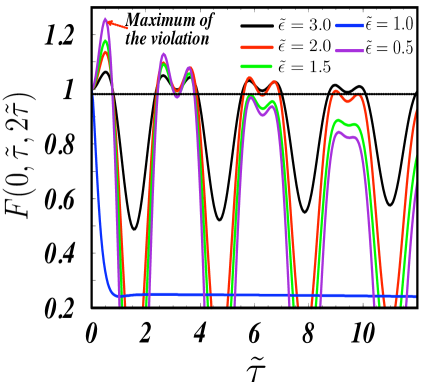
Figure 1: (Color online). LGI-F function at thermal equilibrium, i.e. ΔT~=0Δ~𝑇0\Delta\tilde{T}=0. F(0,τ~,2τ~)𝐹0~𝜏2~𝜏F(0,\tilde{\tau},2\tilde{\tau}) for symmetrical qubits with different splittings and identical bath temperatures T~1=T~2=1.1subscript~𝑇1subscript~𝑇21.1\tilde{T}_{1}=\tilde{T}_{2}=1.1. The LGI is violated whenever F(0,τ~,2τ~)>1𝐹0~𝜏2~𝜏1F(0,\tilde{\tau},2\tilde{\tau})>1.

IV Results and discussions

Although the main idea behind the initial proposal of the LGI was to test macroscopic realism leggett , we will use LGI with a different purpose. As we saw in the discussion leading to LGI, this inequality is never violated in the time evolution of classical systems. Therefore, any system which exhibits any degree of violation to the LGI has some fundamental quantum behavior. We can therefore use LGI violations, similarly to the use of the entanglement of formation and the quantum discord, to identify systems which evolve in some no classical way. This is the reasoning line we will follow from now on.

To illustrate the behavior of the MLGI violation under nonequilibrium thermal conditions we proceed to consider realistic parameters. The set of chosen parameters (in V units), for the results we discuss below, are in the actual experimental range for superconductor qubits ϵ~i5similar-tosubscript~italic-ϵ𝑖5\tilde{\epsilon}_{i}\sim 5 and Γ~103similar-to~Γsuperscript103\tilde{\Gamma}\sim 10^{-3} simmonds while for excitons in biological photosynthetic systems ϵ~i1.4similar-tosubscript~italic-ϵ𝑖1.4\tilde{\epsilon}_{i}\sim 1.4 and Γ~0.4similar-to~Γ0.4\tilde{\Gamma}\sim 0.4 sarovar . First, we analyze results for the equilibrium case, i.e. ΔT~=0Δ~𝑇0\Delta\tilde{T}=0. As plotted in Fig. 1, violations of LGI are still visible up to τ~=10~𝜏10\tilde{\tau}=10 for an equilibrium temperature T~M=T~1=T~2=1.1subscript~𝑇𝑀subscript~𝑇1subscript~𝑇21.1\tilde{T}_{M}=\tilde{T}_{1}=\tilde{T}_{2}=1.1. For weak inter-qubit couplings (ϵ~>1~italic-ϵ1\tilde{\epsilon}>1) the violation of the LGI is small compared with the strong inter-qubit coupling result in the range of 0<τ~<10~𝜏10<\tilde{\tau}<1. However, for 1<τ~<51~𝜏51<\tilde{\tau}<5 that behavior is reversed and the classical non-violation regime prevails (F(0,τ~,2τ~)<1𝐹0~𝜏2~𝜏1F(0,\tilde{\tau},2\tilde{\tau})<1). Moreover, in the weak inter-qubit coupling the LGI violation stands for longer times. By decreasing the qubit splitting ϵ~~italic-ϵ\tilde{\epsilon} the LGI violation is becomes large for short times, as can be seen in Fig.1. For the special case ϵ~=1~italic-ϵ1\tilde{\epsilon}=1, the LGI violation breaks down for any τ~~𝜏\tilde{\tau} and the classical behavior emerges, as should be for a quantum system in contact with an infinite temperature bath as pointed out above.

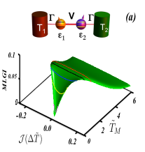
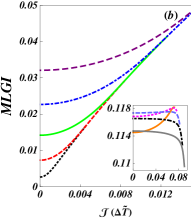
Now, the essential question is: can the LGI violation be enhanced by a temperature gradient or equivalently by a heat current? This is analyzed by plotting in Fig. 2 (a) the MLGI as a function of 𝒥𝒥{\cal J} and the mean temperature T~M=(T~1+T~2)/2subscript~𝑇𝑀subscript~𝑇1subscript~𝑇22\tilde{T}_{M}=(\tilde{T}_{1}+\tilde{T}_{2})/2.

Refer to caption
Refer to caption
Refer to caption
Refer to caption
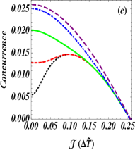
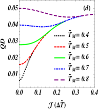
Figure 2: (Color online). Composite quantum system in contact with two separate thermal reservoirs. (a) A 3D plot of the first MLGI (for τ~=π/6~𝜏𝜋6\tilde{\tau}=\pi/6) as a function of mean temperature and heat current for a two-spin chain with ϵ~=3~italic-ϵ3\tilde{\epsilon}=3 and Γ~=0.05~Γ0.05\tilde{\Gamma}=0.05 is shown. (b) Slices taken from the 3D left panel are shown for different T~Msubscript~𝑇𝑀\tilde{T}_{M}. Notice that for the lowest values of T~Msubscript~𝑇𝑀\tilde{T}_{M}, MLGI increases with the application of a temperature gradient. Similar results are shown in the inset for higher mean temperatures: Orange (T~M=2.25subscript~𝑇𝑀2.25\tilde{T}_{M}=2.25), magenta (T~M=2.5subscript~𝑇𝑀2.5\tilde{T}_{M}=2.5), purple (T~M=2.75subscript~𝑇𝑀2.75\tilde{T}_{M}=2.75), black (T~M=3.0subscript~𝑇𝑀3.0\tilde{T}_{M}=3.0), gray (T~M=3.25subscript~𝑇𝑀3.25\tilde{T}_{M}=3.25). A qualitatively similar behavior can be observed for the two-spin chain concurrence (c) and quantum discord (d) as a function of the heat current. The color convention for curves in (b-main figure), (c) and (d) is the same. Since the values of ϵ~~italic-ϵ\tilde{\epsilon} are the same, a symmetric curve is obtained for ΔT~<0.Δ~𝑇0\Delta\tilde{T}<0.

The variation of MLGI vs. heat current (or equivalently temperature gradient) changes its concavity indicating that the enhancement of LGI violations under nonequilibrium thermal conditions is restricted to the low mean temperature sector. This behavior can be understood as a competition of the coherent flip-flop spin processes (dominated by the V𝑉V term) and a temperature dependent decay rate (Γ~Vsubscript~Γ𝑉\tilde{\Gamma}_{V}), as can be deduced from Eq. 24. Since Γ~V<<1much-less-thansubscript~Γ𝑉1\tilde{\Gamma}_{V}<<1, it is possible to obtain an analytical expression for the MLGI as MLGIr23[eπΓ~V6+12eπΓ~V31]similar-to-or-equals𝑀𝐿𝐺𝐼subscript𝑟23delimited-[]superscript𝑒𝜋subscript~Γ𝑉612superscript𝑒𝜋subscript~Γ𝑉31MLGI\simeq r_{23}\left[e^{-\frac{\pi\tilde{\Gamma}_{V}}{6}}+\frac{1}{2}e^{-\frac{\pi\tilde{\Gamma}_{V}}{3}}-1\right], that depends on the product of the stationary spin chain level populations r23subscript𝑟23r_{23} and an effective decay term. For low T~Msubscript~𝑇𝑀\tilde{T}_{M}, and ΔT~<<2T~Mmuch-less-thanΔ~𝑇2subscript~𝑇𝑀\Delta\tilde{T}<<2\tilde{T}_{M}, the population term in the last analytical MLGI expression is much more important than the effective decay indicating that the MLGI starts to grow as the r23subscript𝑟23r_{23} increases for ΔT~=0Δ~𝑇0\Delta\tilde{T}=0. By contrast, for higher T~Msubscript~𝑇𝑀\tilde{T}_{M} it is very easy to demonstrate that r23subscript𝑟23r_{23} decreases faster than the contribution of the effective decay Γ~Vsubscript~Γ𝑉\tilde{\Gamma}_{V} indicating that the decay term dominates and the flip-flop interaction does not contribute appreciably due to the fact that the population of each eigenstate is saturated at 1/4. This is the main reason why moving away from thermal equilibrium the MLGI decreases for high T~Msubscript~𝑇𝑀\tilde{T}_{M}. The non-equilibrium enhancement of spatial quantum coherences in the same spin-chain system, as measured by the concurrence quiroga and QD wu1 , is shown in Fig. 2 (c)-(d), respectively. This correspondence between spatial and temporal correlations extends to a nonequilibrium thermal setting previous observations of a perfect mapping between Bell inequality and LGI reznik .

Our method as applied to the single spin case nori ; huelga (results not shown here) demonstrates that MLGI is not enhanced, rather it is suppressed, when a nonequilibrium temperature gradient is applied. Therefore, a two-qubit system is the smallest spin chain where nonequilibrium enhancement of LGI violations can be observed.

A complete presentation of LGI violations under nonequilibrium conditions is given in Fig.3 (a)
Refer to caption
Refer to caption
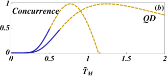
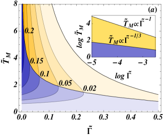
Figure 3: (Color online). (a) Contour plot of MLGI in the (Γ~,T~M)~Γsubscript~𝑇𝑀(\tilde{\Gamma},\tilde{T}_{M}) parameter space for ϵ~=3~italic-ϵ3\tilde{\epsilon}=3. The numbers around the contour lines give the values of the MGLI at ΔT~=0Δ~𝑇0\Delta\tilde{T}=0. Inset: (Γ~,T~M~Γsubscript~𝑇𝑀\tilde{\Gamma},\tilde{T}_{M}) in log-log scales showing power laws for the borderlines between different non-equilibrium MLGI behavior regions. (b) Typical behaviors of concurrence and QD at equilibrium (both normalized to their maximum value), where a blue solid line indicates that a temperature gradient increases the quantum spatial correlation while a yellow dashed line indicates that a temperature gradient decreases the quantum spatial correlation

We point out that thermal nonequilibrium effects on LGI violations can be grouped in three zones in the whole (Γ~,T~M)~Γsubscript~𝑇𝑀(\tilde{\Gamma},\tilde{T}_{M}) parameter space. First, there are no LGI violations, both in equilibrium and nonequilibrium, for sufficiently high Γ~~Γ\tilde{\Gamma} or T~Msubscript~𝑇𝑀\tilde{T}_{M} values, corresponding to the upper right white zone in Fig. 3 (a). This behavior is consistent with the deleterious effect of strong coupling or high temperature on quantum correlations. Second, there is a zone with intermediate values of Γ~~Γ\tilde{\Gamma} and T~Msubscript~𝑇𝑀\tilde{T}_{M} (yellow region in Fig.3 (a) where MLGI>0𝑀𝐿𝐺𝐼0MLGI>0 at thermal equilibrium, but the MLGI starts deteriorating rather than improving as the system is subject to a small temperature gradient. As shown in the inset, where a log-log scale has been used for Γ~~Γ\tilde{\Gamma} and T~Msubscript~𝑇𝑀\tilde{T}_{M}, the numerically determined borderline between the white and yellow zones has a power law expression such that T~MΓ~1similar-tosubscript~𝑇𝑀superscript~Γ1\tilde{T}_{M}\sim\tilde{\Gamma}^{-1}. This simple relation can be easily justified by using our analytical approximation for MLGI, by searching for the (Γ~,T~M)~Γsubscript~𝑇𝑀(\tilde{\Gamma},\tilde{T}_{M}) values yielding to a null value for MLGI at ΔT~=0Δ~𝑇0\Delta\tilde{T}=0. Third, and most importantly, there is a parameter region of low Γ~~Γ\tilde{\Gamma} or T~Msubscript~𝑇𝑀\tilde{T}_{M} values (blue zone in Fig.3 (a) where the equilibrium value of MLGI is further increased as the system is taken out of equilibrium by setting a temperature gradient. The numerically determined borderline between the yellow and blue regions in Fig.3 (a) satisfies also a power law of the form T~MΓ~1/3similar-tosubscript~𝑇𝑀superscript~Γ13\tilde{T}_{M}\sim\tilde{\Gamma}^{-1/3}. This behavior can also be explained by requiring that 2MLGI(ΔT~)2|ΔT~=0=0evaluated-atsuperscript2𝑀𝐿𝐺𝐼superscriptΔ~𝑇2Δ~𝑇00\frac{\partial^{2}MLGI}{\partial(\Delta\tilde{T})^{2}}|_{\Delta\tilde{T}=0}=0, (details of the derivation are given in Appendix B)

Γ~=3π[ϵ~4]3[1(1ϵ~)4]1T~M3~Γ3𝜋superscriptdelimited-[]~italic-ϵ43delimited-[]1superscript1~italic-ϵ41superscriptsubscript~𝑇𝑀3\displaystyle\tilde{\Gamma}=\frac{3}{\pi}\left[\frac{\tilde{\epsilon}}{4}\right]^{3}\left[1-\left(\frac{1}{\tilde{\epsilon}}\right)^{4}\right]\frac{1}{\tilde{T}_{M}^{3}} (25)

in agreement with the numerical results plotted in Fig. 3 (a). Clearly, when the inter-qubit interaction is greater than the energy splitting, no solution for Eq.(25) exists indicating that a requirement for the thermal nonequilibrium enhancement of LGI violations is that spins are in the weak coupling regime. By contrast with two-time quantum correlations, two-point spatial correlations in the steady-state do not depend on the quantum system coupling strength with the thermal baths. However, as shown in Fig.3 (b), the two-spin concurrence and QD also present a nonequilibrium thermal enhancement at low enough temperatures signaling one more time the correspondence between temporal and spatial quantum correlation behaviors. As it has already been documented the QD persists up to larger temperatures as compared with the concurrence.

V Conclusions

In summary, we have provided a microscopic derivation of LGI, for a spin chain coupled to two reservoirs at different temperatures. Nonequilibrium thermal quantum correlations have been analyzed exactly by mapping the original two-interacting spins coupled chain to an equivalent system of two-noninteracting spins, each one of them in contact with a renormalized heat reservoir at an effective temperature. Based on a Kraus-operator approach, we demonstrate that in a certain range of temperature gradients the steady-state LGI violation can be enhanced. The frontiers between different behaviors of the MLGI response to thermal nonequilibrium conditions have been found to be characterized by power laws relating mean temperature of the heat reservoirs and the spin chain coupling strength with the baths. This leads to the interesting feature that nonequilibrium thermal conditions provide the opportunity to enhance not only spatial but also temporal quantum correlations.

Acknowledgements.
We acknowledge Susana Huelga and Neil F. Johnson’s critical readings of the manuscript and Facultad de Ciencias, Vicerrectoría de investigaciones at Universidad de los Andes, for financial support to the project Quantum control of Non-Equilibrium hybrid systems (2012-2014).

Appendix A Time-dependent quantum correlations

We start writing the expression for C(t1,t2)𝐶subscript𝑡1subscript𝑡2C(t_{1},t_{2}), also by simplifying it only in terms of Π+superscriptΠ\Pi^{+} (with Π=IΠ+superscriptΠ𝐼superscriptΠ\Pi^{-}=I-\Pi^{+}). We must do a similar expansion of all the 15 terms as the one we did for the case of unitary evolution of a pure state, after which we obtain the following expression:

C(t1,t2)=12Tr{Π+νμKν(titl)Kμ(tl)ρ0Kμ(tl)Kν(titl)}𝐶subscript𝑡1subscript𝑡212TrsuperscriptΠsubscript𝜈𝜇subscript𝐾𝜈subscript𝑡𝑖subscript𝑡𝑙subscript𝐾𝜇subscript𝑡𝑙subscript𝜌0subscriptsuperscript𝐾𝜇subscript𝑡𝑙subscriptsuperscript𝐾𝜈subscript𝑡𝑖subscript𝑡𝑙\displaystyle C(t_{1},t_{2})=1-2\mathrm{Tr}\left\{\Pi^{+}\sum_{\nu\mu}K_{\nu}(t_{i}-t_{l})K_{\mu}(t_{l})\rho_{0}K^{\dagger}_{\mu}(t_{l})K^{\dagger}_{\nu}(t_{i}-t_{l})\right\}
Tr{νμKν(titl)Π+Kμ(tl)ρ0Kμ(tl)Kν(titl)}Trsubscript𝜈𝜇subscript𝐾𝜈subscript𝑡𝑖subscript𝑡𝑙superscriptΠsubscript𝐾𝜇subscript𝑡𝑙subscript𝜌0subscriptsuperscript𝐾𝜇subscript𝑡𝑙subscriptsuperscript𝐾𝜈subscript𝑡𝑖subscript𝑡𝑙\displaystyle-\mathrm{Tr}\left\{\sum_{\nu\mu}K_{\nu}(t_{i}-t_{l})\Pi^{+}K_{\mu}(t_{l})\rho_{0}K^{\dagger}_{\mu}(t_{l})K^{\dagger}_{\nu}(t_{i}-t_{l})\right\}
Tr{νμKν(titl)Kμ(tl)ρ0Kμ(tl)Π+Kν(titl)}Trsubscript𝜈𝜇subscript𝐾𝜈subscript𝑡𝑖subscript𝑡𝑙subscript𝐾𝜇subscript𝑡𝑙subscript𝜌0subscriptsuperscript𝐾𝜇subscript𝑡𝑙superscriptΠsubscriptsuperscript𝐾𝜈subscript𝑡𝑖subscript𝑡𝑙\displaystyle-\mathrm{Tr}\left\{\sum_{\nu\mu}K_{\nu}(t_{i}-t_{l})K_{\mu}(t_{l})\rho_{0}K^{\dagger}_{\mu}(t_{l})\Pi^{+}K^{\dagger}_{\nu}(t_{i}-t_{l})\right\}
+2Tr{Π+νμKν(titl)Π+Kμ(tl)ρ0Kμ(tl)Kν(titl)}2TrsuperscriptΠsubscript𝜈𝜇subscript𝐾𝜈subscript𝑡𝑖subscript𝑡𝑙superscriptΠsubscript𝐾𝜇subscript𝑡𝑙subscript𝜌0subscriptsuperscript𝐾𝜇subscript𝑡𝑙subscriptsuperscript𝐾𝜈subscript𝑡𝑖subscript𝑡𝑙\displaystyle+2\mathrm{Tr}\left\{\Pi^{+}\sum_{\nu\mu}K_{\nu}(t_{i}-t_{l})\Pi^{+}K_{\mu}(t_{l})\rho_{0}K^{\dagger}_{\mu}(t_{l})K^{\dagger}_{\nu}(t_{i}-t_{l})\right\}
+2Tr{Π+νμKν(titl)Kμ(tl)ρ0Kμ(tl)Π+Kν(titl)}2TrsuperscriptΠsubscript𝜈𝜇subscript𝐾𝜈subscript𝑡𝑖subscript𝑡𝑙subscript𝐾𝜇subscript𝑡𝑙subscript𝜌0subscriptsuperscript𝐾𝜇subscript𝑡𝑙superscriptΠsubscriptsuperscript𝐾𝜈subscript𝑡𝑖subscript𝑡𝑙\displaystyle+2\mathrm{Tr}\left\{\Pi^{+}\sum_{\nu\mu}K_{\nu}(t_{i}-t_{l})K_{\mu}(t_{l})\rho_{0}K^{\dagger}_{\mu}(t_{l})\Pi^{+}K^{\dagger}_{\nu}(t_{i}-t_{l})\right\} (26)

Note that the second term is the probability of measuring +11+1 after evolving ρ0subscript𝜌0\rho_{0} until tlsubscript𝑡𝑙t_{l} and then until tisubscript𝑡𝑖t_{i}, so that it is simply 2p(+ti)-2p(^{+}t_{i}). The third term can be rewritten as follows:

Tr{νKν(titl)[μΠ+Kμ(tl)ρ0Kμ(tl)]Kν(titl)}Trsubscript𝜈subscript𝐾𝜈subscript𝑡𝑖subscript𝑡𝑙delimited-[]subscript𝜇superscriptΠsubscript𝐾𝜇subscript𝑡𝑙subscript𝜌0subscriptsuperscript𝐾𝜇subscript𝑡𝑙subscriptsuperscript𝐾𝜈subscript𝑡𝑖subscript𝑡𝑙\mathrm{Tr}\left\{\sum_{\nu}K_{\nu}(t_{i}-t_{l})\left[\sum_{\mu}\Pi^{+}K_{\mu}(t_{l})\rho_{0}K^{\dagger}_{\mu}(t_{l})\right]K^{\dagger}_{\nu}(t_{i}-t_{l})\right\} (27)

The evolution represented by the Kraus operators is trace-keeping, so that this is the same as

Tr{μΠ+Kμ(tl)ρ0Kμ(tl)}=p(+tl)\mathrm{Tr}\left\{\sum_{\mu}\Pi^{+}K_{\mu}(t_{l})\rho_{0}K^{\dagger}_{\mu}(t_{l})\right\}=p(^{+}t_{l}) (28)

The same happens with the fourth term, so that these two terms add up to 2p(+tl)-2p(^{+}t_{l}). The last two terms can be rewritten as 2g(tl,ti)+h.c.formulae-sequence2𝑔subscript𝑡𝑙subscript𝑡𝑖𝑐2g(t_{l},t_{i})+h.c. if we define

g(tl,ti)=Tr{ρ0νμKμ(tl)Kν(titl)Π+Kν(titl)Π+Kμ(tl)}𝑔subscript𝑡𝑙subscript𝑡𝑖Trsubscript𝜌0subscript𝜈𝜇subscriptsuperscript𝐾𝜇subscript𝑡𝑙subscriptsuperscript𝐾𝜈subscript𝑡𝑖subscript𝑡𝑙superscriptΠsubscript𝐾𝜈subscript𝑡𝑖subscript𝑡𝑙superscriptΠsubscript𝐾𝜇subscript𝑡𝑙g(t_{l},t_{i})=\mathrm{Tr}\left\{\rho_{0}\sum_{\nu\mu}K^{\dagger}_{\mu}(t_{l})K^{\dagger}_{\nu}(t_{i}-t_{l})\Pi^{+}K_{\nu}(t_{i}-t_{l})\Pi^{+}K_{\mu}(t_{l})\right\} (29)

or, alternatively

g(tl,ti)=Tr{νμΠ+Kν(titl)Π+Kμ(tl)ρ0Kμ(tl)Kν(titl)}𝑔subscript𝑡𝑙subscript𝑡𝑖Trsubscript𝜈𝜇superscriptΠsubscript𝐾𝜈subscript𝑡𝑖subscript𝑡𝑙superscriptΠsubscript𝐾𝜇subscript𝑡𝑙subscript𝜌0subscriptsuperscript𝐾𝜇subscript𝑡𝑙subscriptsuperscript𝐾𝜈subscript𝑡𝑖subscript𝑡𝑙\displaystyle g(t_{l},t_{i})=\mathrm{Tr}\left\{\sum_{\nu\mu}\Pi^{+}K_{\nu}(t_{i}-t_{l})\Pi^{+}K_{\mu}(t_{l})\rho_{0}K^{\dagger}_{\mu}(t_{l})K^{\dagger}_{\nu}(t_{i}-t_{l})\right\}
=Tr{Π+νKν(titl)Π+ρ(tl)Kν(titl)}absentTrsuperscriptΠsubscript𝜈subscript𝐾𝜈subscript𝑡𝑖subscript𝑡𝑙superscriptΠ𝜌subscript𝑡𝑙subscriptsuperscript𝐾𝜈subscript𝑡𝑖subscript𝑡𝑙\displaystyle=\mathrm{Tr}\left\{\Pi^{+}\sum_{\nu}K_{\nu}(t_{i}-t_{l})\Pi^{+}\rho(t_{l})K^{\dagger}_{\nu}(t_{i}-t_{l})\right\} (30)

Thus, the correlations can then be written as

C(t1,t2)=12p(+t1)2p(+t2)+4Re[g(t1,t2)]C(t_{1},t_{2})=1-2p(^{+}t_{1})-2p(^{+}t_{2})+4\mathrm{Re}\left[g(t_{1},t_{2})\right] (31)

This expression depends mainly of the correlation function function g𝑔g. It can also be shown that, replacing the Kraus operators with unitary evolution operators, we get exactly the result obtained for pure states. Based on the correlations C𝐶C, the LGI expresion can be written as

F(t1,t2,t3)=C(t1,t2)+C(t2,t3)C(t1,t3)1𝐹subscript𝑡1subscript𝑡2subscript𝑡3𝐶subscript𝑡1subscript𝑡2𝐶subscript𝑡2subscript𝑡3𝐶subscript𝑡1subscript𝑡31\displaystyle F(t_{1},t_{2},t_{3})=C(t_{1},t_{2})+C(t_{2},t_{3})-C(t_{1},t_{3})\leq 1 (32)
F(t1,t2,t3)=14p(+t2)+4Re[g(t1,t2)+g(t2,t3)g(t1,t3)]1\displaystyle F(t_{1},t_{2},t_{3})=1-4p(^{+}t_{2})+4Re\left[g(t_{1},t_{2})+g(t_{2},t_{3})-g(t_{1},t_{3})\right]\leq 1 (33)

Appendix B Power law behaviour of border lines between different ΓTMΓsubscript𝑇𝑀\Gamma-T_{M} regions

First is important to remark that the violation dependes on a population transfer between the two levels: symmetric and antisymetric ρ34subscript𝜌34\rho_{34} and an effective decay ΓvsubscriptΓ𝑣\Gamma_{v}. The violation depends on the product of those terms V=GH𝑉𝐺𝐻V=GH, where G=ρ3,4𝐺subscript𝜌34G=\rho_{3,4} and H𝐻H depends on the effective decay. Before to define all important ingredients it is necessary to gives some algebraic details for temperature:

TM=T1+T22;ΔT=T2T1formulae-sequencesubscript𝑇𝑀subscript𝑇1subscript𝑇22Δ𝑇subscript𝑇2subscript𝑇1\displaystyle T_{M}=\frac{T_{1}+T_{2}}{2};\Delta T=T_{2}-T_{1}
TM+ΔT2=T1;TMΔT2=T2formulae-sequencesubscript𝑇𝑀Δ𝑇2subscript𝑇1subscript𝑇𝑀Δ𝑇2subscript𝑇2\displaystyle T_{M}+\frac{\Delta T}{2}=T_{1};T_{M}-\frac{\Delta T}{2}=T_{2}
T1T2=TM2(ΔT2)2subscript𝑇1subscript𝑇2superscriptsubscript𝑇𝑀2superscriptΔ𝑇22\displaystyle T_{1}T_{2}=T_{M}^{2}-\left(\frac{\Delta T}{2}\right)^{2}
Vmax=GHsubscript𝑉𝑚𝑎𝑥𝐺𝐻\displaystyle V_{max}=GH (34)
G=12(1Δ1Δ2α)𝐺121subscriptΔ1subscriptΔ2𝛼\displaystyle G=\frac{1}{2}\left(1-\Delta_{1}\Delta_{2}\alpha\right) (35)
H=eΓvπ6V+12eΓvπ3V1𝐻superscript𝑒subscriptΓ𝑣𝜋6𝑉12superscript𝑒subscriptΓ𝑣𝜋3𝑉1\displaystyle H=e^{-\frac{\Gamma_{v}\pi}{6V}}+\frac{1}{2}e^{-\frac{\Gamma_{v}\pi}{3V}}-1 (36)
Γv=2Γ(sinh(E1a)Δ1+sinh(E2a)Δ2)subscriptΓ𝑣2Γsubscript𝐸1𝑎subscriptΔ1subscript𝐸2𝑎subscriptΔ2\displaystyle\Gamma_{v}=2\Gamma\left({\frac{\sinh(E_{1}a)}{\Delta_{1}}+\frac{\sinh(E_{2}a)}{\Delta_{2}}}\right) (37)
a=TMT1T2=TMTM2(ΔT2)2=1TM11(ΔT2TM)2𝑎subscript𝑇𝑀subscript𝑇1subscript𝑇2subscript𝑇𝑀superscriptsubscript𝑇𝑀2superscriptΔ𝑇221subscript𝑇𝑀11superscriptΔ𝑇2subscript𝑇𝑀2\displaystyle a=\frac{T_{M}}{T_{1}T_{2}}=\frac{T_{M}}{T_{M}^{2}-\left(\frac{\Delta T}{2}\right)^{2}}=\frac{1}{T_{M}}\frac{1}{1-\left(\frac{\Delta T}{2T_{M}}\right)^{2}} (38)
Δi=2(cosh(Eia)cosh(EiaΔT2TM))subscriptΔ𝑖2subscript𝐸𝑖𝑎subscript𝐸𝑖𝑎Δ𝑇2subscript𝑇𝑀\displaystyle\Delta_{i}=2\left(\cosh(E_{i}a)-\cosh\left(E_{i}a\frac{\Delta T}{2T_{M}}\right)\right) (39)
α=14sinh(E1a)sinh(E2a)𝛼14subscript𝐸1𝑎subscript𝐸2𝑎\displaystyle\alpha=\frac{1}{4\sinh(E_{1}a)\sinh(E_{2}a)} (40)

where V𝑉V denotes the interaction qubit parameter. E2,1=ϵ±Vsubscript𝐸21plus-or-minusitalic-ϵ𝑉E_{2,1}=\epsilon\pm V. We are interested into calculate the curvature of Vmaxsubscript𝑉𝑚𝑎𝑥V_{max}, because it could be give signatures fot the power law behaviour. It is important to refer to one of the main results of LGI, as is Figure 4. The power law behaviour ΓΓ\Gamma vs T𝑇T comes from the fact that a inverse power law that can be obtained when the violation is zero. This calculation is very simple and we do not show here. The main finding of our work is the power law TM3superscriptsubscript𝑇𝑀3T_{M}^{-3}. On the same footing comes from a equilibrium case, where the violations start to decrease , thus, the violations changes its curvature. Therefore it is necessary in both cases to calculate the Vmaxsubscript𝑉𝑚𝑎𝑥V_{max} and Vmax′′superscriptsubscript𝑉𝑚𝑎𝑥′′V_{max}^{\prime\prime} behaviours in the limit of ΔT=0Δ𝑇0\Delta T=0. As a first step we will calculate the second derivative with respect to ΔTΔ𝑇\Delta T and we will take the limit where ΔT0Δ𝑇0\Delta T\rightarrow 0.

d2VmaxdΔT2=G′′H+GH′′superscript𝑑2subscript𝑉𝑚𝑎𝑥𝑑Δsuperscript𝑇2superscript𝐺′′𝐻𝐺superscript𝐻′′\displaystyle\frac{d^{2}V_{max}}{d\Delta T^{2}}=G^{\prime\prime}H+GH^{\prime\prime} (41)

Where the first derivatives gives a zero value in the maximum. First, we need to calculate the second derivative of H𝐻H:

d2HdΔT2superscript𝑑2𝐻𝑑Δsuperscript𝑇2\displaystyle\frac{d^{2}H}{d\Delta T^{2}} =\displaystyle= π6V[eΓvπ6V+eΓvπ3V]d2ΓvdΔT2𝜋6𝑉delimited-[]superscript𝑒subscriptΓ𝑣𝜋6𝑉superscript𝑒subscriptΓ𝑣𝜋3𝑉superscript𝑑2subscriptΓ𝑣𝑑Δsuperscript𝑇2\displaystyle-\frac{\pi}{6V}\left[e^{-\frac{\Gamma_{v}\pi}{6V}}+e^{-\frac{\Gamma_{v}\pi}{3V}}\right]\frac{d^{2}\Gamma_{v}}{d\Delta T^{2}} (43)

Next we have to calculate the ΓV′′superscriptsubscriptΓ𝑉′′\Gamma_{V}^{{}^{\prime\prime}} term.

d2ΓvdΔT2superscript𝑑2subscriptΓ𝑣𝑑Δsuperscript𝑇2\displaystyle\frac{d^{2}\Gamma_{v}}{d\Delta T^{2}} =\displaystyle= 2Γa2{E12TM(aΔTTMΔTΔ1ΔTΔ12dΔ1dΔT+1Δ1)cosh(E1a)+(E1aΔT)24Δ1TM2sinh(E1a)\displaystyle 2\Gamma a^{2}\left\{\frac{E_{1}}{2T_{M}}\left(a\frac{\Delta T}{T_{M}}\frac{\Delta T}{\Delta_{1}}-\frac{\Delta T}{\Delta_{1}^{2}}\frac{d\Delta_{1}}{d\Delta T}+\frac{1}{\Delta_{1}}\right)\cosh(E_{1}a)+\frac{(E_{1}a\Delta T)^{2}}{4\Delta_{1}T_{M}^{2}}\sinh(E_{1}a)-\right. (46)
E12ΔTTMdΔ1dΔT1Δ12cosh(E1a)+2sinh(E1a)Δ1(1aΔ1dΔ1dΔT)2sinh(E1a)(aΔ1)2d2Δ1dΔT2subscript𝐸12Δ𝑇subscript𝑇𝑀𝑑subscriptΔ1𝑑Δ𝑇1superscriptsubscriptΔ12subscript𝐸1𝑎2subscript𝐸1𝑎subscriptΔ1superscript1𝑎subscriptΔ1𝑑subscriptΔ1𝑑Δ𝑇2subscript𝐸1𝑎superscript𝑎subscriptΔ12superscript𝑑2subscriptΔ1𝑑Δsuperscript𝑇2\displaystyle\left.\frac{E_{1}}{2}\frac{\Delta T}{T_{M}}\frac{d\Delta_{1}}{d\Delta T}\frac{1}{\Delta_{1}^{2}}\cosh(E_{1}a)+\frac{2\sinh(E_{1}a)}{\Delta_{1}}\left(\frac{1}{a\Delta_{1}}\frac{d\Delta_{1}}{d\Delta T}\right)^{2}-\frac{\sinh(E_{1}a)}{(a\Delta_{1})^{2}}\frac{d^{2}\Delta_{1}}{d\Delta T^{2}}\right.
+12}\displaystyle\left.+1\rightarrow 2\frac{}{}\right\}

Second, we calculate de second derivative of G

G′′=12(Δ1′′Δ2α+Δ1Δ2′′α+Δ1Δ2α′′)superscript𝐺′′12superscriptsubscriptΔ1′′subscriptΔ2𝛼subscriptΔ1superscriptsubscriptΔ2′′𝛼subscriptΔ1subscriptΔ2superscript𝛼′′\displaystyle G^{\prime\prime}=-\frac{1}{2}(\Delta_{1}^{\prime\prime}\Delta_{2}\alpha+\Delta_{1}\Delta_{2}^{\prime\prime}\alpha+\Delta_{1}\Delta_{2}\alpha^{\prime\prime}) (48)

Next we have to calculate de second derivative of α𝛼\alpha

d2αdΔT2superscript𝑑2𝛼𝑑Δsuperscript𝑇2\displaystyle\frac{d^{2}\alpha}{d\Delta T^{2}} =\displaystyle= a2TM2{(αaΔT)22TM[(E12+E22)sinh(E1a)sinh(E2a)+2E1E2cosh(E2a)cosh(E1a)]\displaystyle-\frac{a^{2}}{T_{M}^{2}}\left\{\frac{(\alpha a\Delta T)^{2}}{2T_{M}}\left[(E_{1}^{2}+E_{2}^{2})\sinh(E_{1}a)\sinh(E_{2}a)+2E_{1}E_{2}\cosh(E_{2}a)\cosh(E_{1}a)\right]\right. (49)
\displaystyle- TMadαdΔT(2TMαadαdΔT+ΔT)+2α2TM[E1cosh(E1a)sinh(E2a)+E2cosh(E2a)sinh(E1a)]}\displaystyle\frac{T_{M}}{a}\frac{d\alpha}{d\Delta T}\left(\frac{2T_{M}}{\alpha a}\frac{d\alpha}{d\Delta T}+\Delta T\right)\left.+2\alpha^{2}T_{M}\left[E_{1}\cosh(E_{1}a)\sinh(E_{2}a)+E_{2}\cosh(E_{2}a)\sinh(E_{1}a)\right]\right\} (50)

The point of interest is to take the limit when ΔT=0Δ𝑇0\Delta T=0 for the second derivatives of ΔisubscriptΔ𝑖\Delta_{i} and ΓΓ\Gamma.

d2ΔidΔT2|ΔT=0evaluated-atsuperscript𝑑2subscriptΔ𝑖𝑑Δsuperscript𝑇2Δ𝑇0\displaystyle\frac{d^{2}\Delta_{i}}{d\Delta T^{2}}|_{\Delta T=0} =\displaystyle= a2[EiTMsinh(Eia)(Eia)221aTMcosh(EiaΔT2TM)]superscript𝑎2delimited-[]subscript𝐸𝑖subscript𝑇𝑀subscript𝐸𝑖𝑎superscriptsubscript𝐸𝑖𝑎221𝑎subscript𝑇𝑀subscript𝐸𝑖𝑎Δ𝑇2subscript𝑇𝑀\displaystyle a^{2}\left[\frac{E_{i}}{T_{M}}\sinh(E_{i}a)-\frac{(E_{i}a)^{2}}{2}\frac{1}{aT_{M}}\cosh\left(\frac{E_{i}a\Delta T}{2T_{M}}\right)\right] (51)
=\displaystyle= a2EiTM[sinh(Eia)Eia2]=EiTM3[sinh(EiTM)Ei2TM]superscript𝑎2subscript𝐸𝑖subscript𝑇𝑀delimited-[]subscript𝐸𝑖𝑎subscript𝐸𝑖𝑎2subscript𝐸𝑖superscriptsubscript𝑇𝑀3delimited-[]subscript𝐸𝑖subscript𝑇𝑀subscript𝐸𝑖2subscript𝑇𝑀\displaystyle\frac{a^{2}E_{i}}{T_{M}}\left[\sinh(E_{i}a)-\frac{E_{i}a}{2}\right]=\frac{E_{i}}{T_{M}^{3}}\left[\sinh\left(\frac{E_{i}}{T_{M}}\right)-\frac{E_{i}}{2T_{M}}\right] (52)
d2ΓvdΔT2|ΔT=0evaluated-atsuperscript𝑑2subscriptΓ𝑣𝑑Δsuperscript𝑇2Δ𝑇0\displaystyle\frac{d^{2}\Gamma_{v}}{d\Delta T^{2}}|_{\Delta T=0} =\displaystyle= 2Γa2{E12TMΔ1cosh(E1a)sinh(E1a)(aΔ1)2d2Δ1dΔT2+12}2Γsuperscript𝑎2subscript𝐸12subscript𝑇𝑀subscriptΔ1subscript𝐸1𝑎subscript𝐸1𝑎superscript𝑎subscriptΔ12superscript𝑑2subscriptΔ1𝑑Δsuperscript𝑇212absentabsent\displaystyle 2\Gamma a^{2}\left\{\frac{E_{1}}{2T_{M}\Delta_{1}}\cosh(E_{1}a)-\frac{\sinh(E_{1}a)}{(a\Delta_{1})^{2}}\frac{d^{2}\Delta_{1}}{d\Delta T^{2}}+1\rightarrow 2\frac{}{}\right\} (53)
=\displaystyle= Γ2TM2{E1TMcosh(E1TM)cosh(E1TM)1+E1TMsinh(E1TM)(cosh(E1TM)1)2[E12TMsinh(E1TM)]+12}Γ2superscriptsubscript𝑇𝑀2subscript𝐸1subscript𝑇𝑀subscript𝐸1subscript𝑇𝑀subscript𝐸1subscript𝑇𝑀1subscript𝐸1subscript𝑇𝑀subscript𝐸1subscript𝑇𝑀superscriptsubscript𝐸1subscript𝑇𝑀12delimited-[]subscript𝐸12subscript𝑇𝑀subscript𝐸1subscript𝑇𝑀12absentabsent\displaystyle\frac{\Gamma}{2T_{M}^{2}}\left\{\frac{E_{1}}{T_{M}}\frac{\cosh(\frac{E_{1}}{T_{M}})}{\cosh(\frac{E_{1}}{T_{M}})-1}+\frac{E_{1}}{T_{M}}\frac{\sinh(\frac{E_{1}}{T_{M}})}{(\cosh(\frac{E_{1}}{T_{M}})-1)^{2}}\left[\frac{E_{1}}{2T_{M}}-\sinh\left(\frac{E_{1}}{T_{M}}\right)\right]+1\rightarrow 2\frac{}{}\right\} (54)

With those ingredientes calculated before and After a long algebra and defining xi=Ei2TMsubscript𝑥𝑖subscript𝐸𝑖2subscript𝑇𝑀x_{i}=\frac{E_{i}}{2T_{M}}, G′′superscript𝐺′′G^{\prime\prime}, in the limit where ΔT=0Δ𝑇0\Delta T=0, can be written as:

H′′=π3V[1Γπ2V]Γ2TM2i=12xi[xitanh(xi)]cosh(xi)sinh3(xi)superscript𝐻′′𝜋3𝑉delimited-[]1Γ𝜋2𝑉Γ2superscriptsubscript𝑇𝑀2superscriptsubscript𝑖12subscript𝑥𝑖delimited-[]subscript𝑥𝑖subscript𝑥𝑖subscript𝑥𝑖superscript3subscript𝑥𝑖\displaystyle H^{\prime\prime}=-\frac{\pi}{3V}\left[1-\frac{\Gamma\pi}{2V}\right]\frac{\Gamma}{2T_{M}^{2}}\sum_{i=1}^{2}x_{i}\left[x_{i}-\tanh(x_{i})\right]\frac{\cosh(x_{i})}{\sinh^{3}(x_{i})} (56)

To calculate the second derivative is necesary to evaluate G𝐺G and H𝐻H at ΔT=0Δ𝑇0\Delta T=0. First G𝐺G:

G|ΔT=0evaluated-at𝐺Δ𝑇0\displaystyle G|_{\Delta T=0} =\displaystyle= 12(1Δ1Δ2α)121subscriptΔ1subscriptΔ2𝛼\displaystyle\frac{1}{2}\left(1-\Delta_{1}\Delta_{2}\alpha\right) (57)
=\displaystyle= 12[1tanh(x1)tanh(x2)]12delimited-[]1subscript𝑥1subscript𝑥2\displaystyle\frac{1}{2}\left[1-\tanh(x_{1})\tanh(x_{2})\right] (58)

Second H𝐻H. To calculate it, we need Γv|ΔT=0evaluated-atsubscriptΓ𝑣Δ𝑇0\Gamma_{v}|_{\Delta T=0}. We assume the limit of low average temperatures

Γv|ΔT=0evaluated-atsubscriptΓ𝑣Δ𝑇0\displaystyle\Gamma_{v}|_{\Delta T=0} \displaystyle\approx 2Γ2Γ\displaystyle 2\Gamma (60)
H|ΔT=0evaluated-at𝐻Δ𝑇0\displaystyle H|_{\Delta T=0} =\displaystyle= eΓvπ6V+12eΓvπ3V1superscript𝑒subscriptΓ𝑣𝜋6𝑉12superscript𝑒subscriptΓ𝑣𝜋3𝑉1\displaystyle e^{-\frac{\Gamma_{v}\pi}{6V}}+\frac{1}{2}e^{-\frac{\Gamma_{v}\pi}{3V}}-1 (61)
=\displaystyle= 12(14Γπ3V)1214Γ𝜋3𝑉\displaystyle\frac{1}{2}\left(1-\frac{4\Gamma\pi}{3V}\right) (62)

The main objective is to calculate the second derivative of Vmaxsubscript𝑉𝑚𝑎𝑥V_{max}, when ΔT0Δ𝑇0\Delta T\rightarrow 0. We define xi=EiTMsubscript𝑥𝑖subscript𝐸𝑖subscript𝑇𝑀x_{i}=\frac{E_{i}}{T_{M}} and To explain the concavity we need:

d2VdΔT2superscript𝑑2𝑉𝑑Δsuperscript𝑇2\displaystyle\frac{d^{2}V}{d\Delta T^{2}} =\displaystyle= G′′H+GH′′superscript𝐺′′𝐻𝐺superscript𝐻′′\displaystyle G^{\prime\prime}H+GH^{\prime\prime} (63)

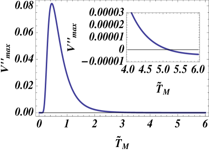
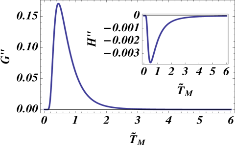
Clearly the second derivative of H𝐻H is always negative, allowing that we can find Vmaxsubscript𝑉𝑚𝑎𝑥V_{max} can be zero. We show a plot of both curvatures
Refer to caption
Refer to caption
Figure 4: Second derivatives of Vmaxsubscript𝑉𝑚𝑎𝑥V_{max}, G and H with respect to ΔTΔ𝑇\Delta T, for ϵ~=3~italic-ϵ3\tilde{\epsilon}=3 and Γ~=0.01~Γ0.01\tilde{\Gamma}=0.01

This means that the second derivative of the maximum violation depends on which effect is stronger between the convexity of G𝐺G and the concavity of H𝐻H. We therefore show plots of both curvatures and their sum in figure 4, along with a plot of the second derivative of Vmaxsubscript𝑉𝑚𝑎𝑥V_{max}. Fig.4 shows that the second derivative of G𝐺G is always positive, whereas the second derivative of H𝐻H is always negative. The result is that the second derivative of Vmaxsubscript𝑉𝑚𝑎𝑥V_{max} depends on which of these two effects is prevalent. For low Tmsubscript𝑇𝑚T_{m}, G′′superscript𝐺′′G^{\prime\prime} increases very fast, so that Vmax′′subscriptsuperscript𝑉′′𝑚𝑎𝑥V^{\prime\prime}_{max} is positive. However, G′′superscript𝐺′′G^{\prime\prime} also decays faster than H′′superscript𝐻′′H^{\prime\prime} with high Tmsubscript𝑇𝑚T_{m}, so that the fact that H′′<0superscript𝐻′′0H^{\prime\prime}<0 is prevalent for high mean temperatures. We can see this in Fig.4, left panel, where the inset shows that the second derivative crosses the horizontal axis at around Tm=5subscript𝑇𝑚5T_{m}=5.

The conclusion is that for low temperatures the effect of G𝐺G is much more important than the effect of H. This is the main reason for the increased violations out of equilibrium. On the other hand, as the temperature increases the effect of G𝐺G vanishes, which is not surprising since the population of each eigenstate tends to 1414\frac{1}{4}, while the effect of H𝐻H remains. This is the reason why moving away from equilibrium reduces the maximum violation to the LGI for high temperatures.

To justify the numerical calculations, we approximate at first order tanh(x)=exexex+ex2x2+x2𝑥superscript𝑒𝑥superscript𝑒𝑥superscript𝑒𝑥superscript𝑒𝑥2𝑥2superscript𝑥2\tanh(x)=\frac{e^{x}-e^{-x}}{e^{x}+e^{-x}}\approx\frac{2x}{2+x^{2}}, that is valid for the limit of |Ei2TM|<1subscript𝐸𝑖2subscript𝑇𝑀1|\frac{E_{i}}{2T_{M}}|<1. Additionally, we take into account the sinh(x)xproportional-to𝑥𝑥\sinh(x)\propto x and cosh(x)1+x2/2proportional-to𝑥1superscript𝑥22\cosh(x)\propto 1+x^{2}/2 As we are working in the Markovian limit and to be consistent with the linblad approximation, terms proportional to Γ2superscriptΓ2\Gamma^{2}, goes to zero. After a long algebra we get the following equation

x13x2+x23x1superscriptsubscript𝑥13subscript𝑥2superscriptsubscript𝑥23subscript𝑥1\displaystyle x_{1}^{3}x_{2}+x_{2}^{3}x_{1} =\displaystyle= 2π3ΓV(x1+x2)(4+2(x12+x22)+x1x2(x1x21))2𝜋3Γ𝑉subscript𝑥1subscript𝑥242superscriptsubscript𝑥12superscriptsubscript𝑥22subscript𝑥1subscript𝑥2subscript𝑥1subscript𝑥21\displaystyle\frac{2\pi}{3}\frac{\Gamma}{V}(x_{1}+x_{2})(4+2(x_{1}^{2}+x_{2}^{2})+x_{1}x_{2}(x_{1}x_{2}-1))
\displaystyle\approx 8π3ΓV(x1+x2)8𝜋3Γ𝑉subscript𝑥1subscript𝑥2\displaystyle\frac{8\pi}{3}\frac{\Gamma}{V}(x_{1}+x_{2})
E13E2TM4+E23E1TM4superscriptsubscript𝐸13subscript𝐸2superscriptsubscript𝑇𝑀4superscriptsubscript𝐸23subscript𝐸1superscriptsubscript𝑇𝑀4\displaystyle\frac{E_{1}^{3}E_{2}}{T_{M}^{4}}+\frac{E_{2}^{3}E_{1}}{T_{M}^{4}} =\displaystyle= 43π3ΓV(E1TM+E2TM)superscript43𝜋3Γ𝑉subscript𝐸1subscript𝑇𝑀subscript𝐸2subscript𝑇𝑀\displaystyle\frac{4^{3}\pi}{3}\frac{\Gamma}{V}(\frac{E_{1}}{T_{M}}+\frac{E_{2}}{T_{M}})
343πE1E2E1+E2(E12+E22)1TM33superscript43𝜋subscript𝐸1subscript𝐸2subscript𝐸1subscript𝐸2superscriptsubscript𝐸12superscriptsubscript𝐸221superscriptsubscript𝑇𝑀3\displaystyle\frac{3}{4^{3}\pi}\frac{E_{1}E_{2}}{E_{1}+E_{2}}(E_{1}^{2}+E_{2}^{2})\frac{1}{T_{M}^{3}} =\displaystyle= ΓVΓ𝑉\displaystyle\frac{\Gamma}{V}

By normalizing to the interaction term V𝑉V

Γ=343πϵ41ϵ1TM3Γ3superscript43𝜋superscriptitalic-ϵ41italic-ϵ1superscriptsubscript𝑇𝑀3\displaystyle\Gamma=\frac{3}{4^{3}\pi}\frac{\epsilon^{4}-1}{\epsilon}\frac{1}{T_{M}^{3}} (65)

References

  • (1) J. S. Bell, Physics 1, 195 (1964).
  • (2) A. J. Leggett and A. Garg, Phys. Rev. Lett. 54, 857 (1985).
  • (3) J. P. Paz and G. Mahler, Phys. Rev. Lett. 71, 3235 (1993).
  • (4) S. F. Huelga, T. W. Marshall and E. Santos, Phys. Rev. A54, 1798 (1996).
  • (5) J. Kofler and C. Brukner, Phys. Rev. Lett. 101, 090403 (2008).
  • (6) N. Lambert, R. Johansson and F. Nori, Phys. Rev. B84, 245421 (2011).
  • (7) A. Palacios-Laloy, F. Mallet, F. Nguyen, P. Bertet, D. Vion, D. Esteve and A. N. Korotkov, Nature Phys. 6, 442 (2010).
  • (8) M. E. Goggin, M. P. Almeida, M. Barbieri, B. P. Lanyon, J. L. OB́rien, A. G. White and G. J. Pryde, Proc. Acad. Nat. Sci. 108, 1256 (2011).
  • (9) G. C. Knee, S. Simmons, E. M. Gauger, J. J.L. Morton, H. Riemann, N. V. Abrosimov, P. Becker, H.-J. Pohl, K. M. Itoh, M. L.W. Thewalt, G. A. D. Briggs and S. C. Benjamin, Nat. Commun. 3:606 doi:10.1038/ncomms1614 (2012).
  • (10) A. N. Jordan, A. N. Korotkov and M. Büttiker, Phys. Rev. Lett. 97, 026805 (2006)
  • (11) V. Athalye, S. Singha Roy and T. S. Mahesh, Phys. Rev. Lett. 107, 130402 (2008).
  • (12) G. Waldherr, P. Neumann, S. F. Huelga, F. Jelezko and J. Wrachtrup, Phys. Rev. Lett. 107, 090401 (2011).
  • (13) J.-S Xu, C.-F. Li, X.-B. Zouand and G.-C. Guo, Sci. Rep. 1, 101; doi:10.1038/srep00101 (2011); J.-S. Xu, C.-F. Li, C.-J. Zhang, X.-Y. Xu, Y.-S. Zhang and G.-C. Guo, Phys. Rev. A82, 042328 (2010).
  • (14) J. Dressel,, C. J. Broadbent, J. C. Howell and A. N. Jordan, Phys. Rev. Lett. 106, 040402 (2011).
  • (15) L. Quiroga, F. J. Rodríguez, M. E. Ramírez and R. París, Phys. Rev. A75, 032308 (2007).
  • (16) A. Polkovnikov, K. Sengupta, A. Silva and M.Vengalattore, Rev. Mod. Phys. 83, 863 (2011).
  • (17) M. A. Cazalilla, A. Iucci and M-C- Chung, Phys. Rev. E85, 011133 (2012).
  • (18) M.B. Plenio and S. Huelga, Phys. Rev. Lett. 88, 197901 (2002).
  • (19) I.Sinayski, F.Petruccione and D.Burgarth, Phys. Rev. A78, 062301 (2008).
  • (20) N. Lambert, R. Aguado and T. Brandes, Phys. Rev. B75, 045340 (2007).
  • (21) L.-A.Wu and D.Segal, Phys. Rev. A84, 012319 (2011).
  • (22) M. Greiner, O. Mandel, T. Hansch and I. Bloch, Nature 419, 51 (2002).
  • (23) R.W. Simmonds, K.M. Lang, D. A. Hite, S. Nam, D. P. Pappas and John M. Martinis, Phys. Rev. Lett. 93, 077003 (2004).
  • (24) M. Sarovar, A. Ishizaki, G. R. Fleming and K. B. Whaley, Nat. Phys. 6, 462 (2010).
  • (25) M. Scully, Phys. Rev. Lett. 87, 220601 (2001).
  • (26) F. Giazotto, and M. Martínez Pérez, Nature 492, 401 (2012).
  • (27) D. Avis, P. Hayden, and M. M. Wilde, Phys. Rev. A82, 030102(R) (2010).
  • (28) K. Kraus, States, Effects and Operations: Fundamental Notions of Quantum Theory. (Springer Verlag, 1983).
  • (29) S.Marcovitch and B.Reznik, quant-ph/1107.2186.