On estimating cosmology-dependent covariance matrices

Abstract

We describe a statistical model to estimate the covariance matrix of matter tracer two-point correlation functions with cosmological simulations. Assuming a fixed number of cosmological simulation runs, we describe how to build a ‘statistical emulator’ of the two-point function covariance over a specified range of input cosmological parameters. Because the simulation runs with different cosmological models help to constrain the form of the covariance, we predict that the cosmology-dependent covariance may be estimated with a comparable number of simulations as would be needed to estimate the covariance for fixed cosmology. Our framework is a necessary first step in planning a simulations campaign for analyzing the next generation of cosmological surveys.

1 Introduction

Cosmological large-scale structure statistics contain valuable information about many cosmological parameters. Accurate parameter inference from large-scale structure observations requires a model for the sample variance distribution of the observed statistics, for example the uncertainties and correlations between angular scales in the galaxy two-point correlation function. Often, the sample variance distribution is assumed to be multivariate Gaussian, requiring specification of only a covariance matrix of the cosmological two-point functions. While the covariance of the two-point function is known for a Gaussian field, effects of survey masks, galaxy clustering bias, and nonlinear gravitational evolution require many simulated realizations of the survey via $N$-body codes to accurately predict the covariance structure. Ref. [1] recently showed that errors in covariance estimates propagate into increased cosmological parameter errors, which have the same effect as a reduction in the survey area. Near-term surveys will require at least $10^{4}$ simulation realizations to prevent effective survey area losses larger than 10%. But, the computational requirements for covariance estimation will be even more challenging than forecasted in Ref. [1] because the cosmology dependence of the covariance is likely to become important as cosmological parameter constraints shrink in future surveys [2, 3].

In some analyses, the covariance matrix was estimated from the data using resampling methods such as the Jackknife or bootstrap. This has two large disadvantages. First, [4] showed that a variety of resampling methods underestimate both the variances and correlations compared to those derived from many simulation realizations. Second, any data-derived covariance estimator necessarily ignores the cosmology-dependence in the covariance which can significantly bias results [2].

In this paper we aim to determine how many cosmological simulations are required to achieve a target uncertainty in the covariance of the two-point correlations of mass density tracers. We also show how the number of simulation runs can be reduced over the brute force approach by exploiting the smooth variation of the covariance components as a function of standard cosmological parameters in a simulation emulator.

We briefly argue for the need to model the cosmology dependence of the covariance in Section 2, although this has also been established in the literature [2, 3]. In Section 3 we specify the statistical model for the cosmology-dependent covariances that allows estimation of covariances with a minimal number of simulations. In Section 4 we apply the Fisher matrix to forecast the uncertainties in covariance matrix elements as functions of the number of cosmological simulations run. We summarize our main conclusion in Section 5 that it is more efficient to simultaneously model the CDC than run many simulation realizations at several fixed cosmological models. We also briefly describe the halo model used in this analysis and assess its accuracy the Appendix.

2 Why cosmology-dependent covariances?

To motivate a two-point statistic covariance emulator, it is helpful to understand how cosmological parameter inference is affected by the cosmology dependence of the covariance. First, there is an issue of data interpretation: When comparing a model to data is it more helpful to ascribe uncertainties to the data (i.e. from observational limitations) or the model (i.e. from the statistical formulation of the statistics that are observed, commonly referred to as ‘sample variance’)? Second, we should determine how biased our parameter constraints could be if we erroneously ignore the cosmology dependence of the covariance. This latter issue was already addressed in [2] who showed that the inferred parameter constraints can change by many standard deviations in some cosmic shear scenarios and can also be biased. We leave similar predictions using our covariance emulator to future work.

As stated previously, estimating the covariance model from the data tends to underestimate the uncertainties [4] when compared with ensembles of simulated observations. Simulating the error on the model is then the preferred method, however, the model error is itself often model dependent.

For example, consider $N$ observed samples $x_{i}$ from a one-dimensional zero-mean Gaussian distribution where we aim to estimate the standard deviation of the distribution. The maximum likelihood estimator for the standard deviation is,

$$\hat{\sigma}^{2}=\frac{1}{N}\sum_{i}x_{i}^{2}.$$ (2.1)

This estimator has an error,

$${\rm var}\left(\hat{\sigma}^{2}\right)=\frac{(2N-1)\sigma^{2}}{N^{2}},$$ (2.2)

so the error on the estimator is also dependent on the value of the model parameter $\sigma^{2}$. This is a simple example, but the same principle holds for many cosmological estimators.

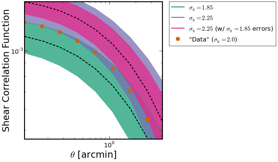
We show an example of parameter-dependent errors on the angular correlation function in Figure 1 when the parameter is the square-root of the amplitude of the two-point function, $\sigma_{8}$. In this example, the data points are generated with $\sigma_{8}=2$ (for illustration only) and are consistent with models that have $\sigma_{8}=1.85$ or $2.25$ when the proper error is used. However, if one were to erroneously assign the errors for $\sigma_{8}=1.85$ to models with varying $\sigma_{8}$ in the mean correlation function (i.e. a model-independent error), the model with the larger true variance would be incorrectly excluded by the data. This situation always arises when assuming fixed errors for cosmological models with different $\sigma_{8}$ (although at a less obvious level for observationally consistent values of $\sigma_{8}<1$). The same principle applies to inference of other cosmological parameters as well.

Figure 1: A cartoon example illustrates how parameter-dependent model errors can be important. A given set of observations, orange points, may be well fit by a model with a small amplitude and smaller model errors (green shaded region) or by a larger amplitude model that also has larger model errors (purple shaded region). If the errors from the model with the smaller amplitude are erroneously assumed to hold for all models we get the magenta band around the higher amplitude model; leading to a worse model fit to the orange data points.

3 Covariance matrix emulator and simulation design

The covariance matrices of large-scale structure probes, $\mathsf{C}$ are typically estimated by running many $N$-body simulations with different pseudo-random number seeds in the initial conditions and constructing a sample covariance estimator from the outputs. This is a computationally intensive task, requiring $10^{4}$ $N$-body simulations to reduce the errors in the covariance below other systematic uncertainties for current surveys and several fold for surveys of the future. These simulations must also be run for different cosmologies in order to properly give unbiased constraints. We address both of these issues with a statistical emulator described in this section that allows for a reduction in the number of simulations required as well as linking together the simulations run at different cosmologies.

We consider $N_{r}\equiv\sum_{i=1}^{n_{d}}n_{r,i}$ simulations run at $n_{d}$ points in parameter space with $n_{r,i}$ independent simulation realizations at each point. For each simulation a summary statistic $\mathbf{y}^{i}_{k}$ (such as the power spectrum or correlation function) is computed (where $k=1,\dots,n_{r,i}$). Given the set of $\mathbf{y}^{i}_{k}$, statistics we now describe how to estimate a model for the cosmology-dependent covariance (CDC) by means of a ‘simulation emulator’.

Simulation emulators have been successfully developed to model the mean matter power spectrum over a six-dimensional cosmological parameter space at high precision [5] and have been applied successfully to problems where the input parameters are less well-constrained [6, 7, 8, 9].

An emulator is specified in 2 steps. The ‘simulation design’ defines at which points in cosmological parameter space $N$-body simulations will be run to calibrate the emulator. The ‘emulation’ step consists of calibrating a statistical model to interpolate the outputs of the simulation design runs to new points in parameter space.

The first step in building a simulation design is choosing the points in parameter space where simulations will be run. The Orthogonal Array Latin Hypercube has proven to be a successful algorithm for choosing design points (but see also the improvements in [10]).

Given specified design points, we then have to decide how many simulation realizations to run at each design point. We could require many simulation realizations at each design point if we need to construct a converged sample covariance estimator. However, with a careful parameterization of the covariance, we can use the simulation runs at all design points simultaneously to jointly constrain the covariance model at each design point.

We achieve our goal in several steps with four features of the covariance emulator that all contribute to improve the estimate of the CDC over a brute-force sample covariance estimator,

1. a careful decomposition of the two-point covariance matrix,

2. a specification of orthogonal basis functions to decorrelate the covariance’s components,

3. optimized Gaussian Process parameters derived from the ensemble of simulation runs,

4. calibration of the emulator to constrain the decorrelated mode amplitudes of the covariance matrix components.

Briefly, we first decompose our matrices using the Generalized Cholesky Decomposition to produce values that are easily emulated. Second, we create basis functions from these values using Principal Component Analysis (PCA). Third we fit (via maximum-likelihood) Gaussian Process parameters to link together the different cosmologies in the simulation design. Finally, we constrain our PCA mode amplitudes using the Gaussian Process.

An important consideration that we neglect in this paper is whether a (potentially noisy) sample covariance estimator is first needed at each design point before the covariance emulator can be constructed. We avoid this issue by using an analytic model for the covariances, but Ref. [11] showed that sample covariance estimates might not be needed at any stage in the calculation. We will explore this further in a later publication.

3.1 Covariance matrix decomposition

We use the Generalized Cholesky Decomposition (GCD) to decompose the covariance matrices [following 12, 13, 14], which is alternately written in the following forms,

$$\mathsf{C} =\mathsf{L}\mathsf{D}\mathsf{L}^{T}$$ (3.1)

$$\mathsf{C}^{-1} =\mathsf{T}^{T}\mathsf{D}^{-1}\mathsf{T},\qquad\mathsf{T}\equiv\mathsf{L}^{-1},$$ (3.2)

where $\mathsf{T}$ is a lower-triangular matrix with ones on the diagonal and $\mathsf{D}$ is a diagonal semi-positive definite matrix. The primary utility of the GCD for our purposes is that a positive definite covariance matrix, $\mathsf{C}$, is guaranteed as long as all diagonal entries of $\mathsf{D}$ are positive, for any real values $\phi$ in the lower triangular components of $\mathsf{T}$. We can therefore interpolate unconstrained values of $\phi$ and $\ln\mathsf{D}$ over the cosmological parameter design space.

We will index the GCD components at each simulation design point with $i=1,\dots,n_{d}$. Assuming the two-point function has $n_{b}$ bins, we label the non-trivial components of $\mathsf{T}$ as [12],

$$\mathsf{T}^{i}_{j\ell}=-\phi_{jl}^{i}\quad{\rm for}\,2\leq j\leq n_{b},\,\ell=1,\dots,j-1.$$ (3.3)

Similarly, we label the diagonal components of $\mathsf{D}$ as,

$$\mathsf{D}_{jj}^{i}=\exp(d^{i}_{j})\quad{\rm for}\,1\leq j\leq n_{b}.$$ (3.4)

3.2 Basis functions

The GCD provides a method to separate the $n_{b}(n_{b}+1)/2$ unique components of the covariance matrix into a computationally convenient form. We can further improve the covariance estimation by reducing the number of components that must be modeled as functions of cosmology. At the same time, we can use all the simulation runs, with all cosmological inputs, to determine common structures in the covariance matrices.

Following the emulator construction in [11, 5], we proceed by extracting the components of $\ln\mathsf{D}$ and $\mathsf{T}$ into separate vectors for each design point, stack these vectors for all design points into an $n_{y}\times n_{d}$ array (where $n_{y}$ is either equal to $n_{b}$ or $n_{b}(n_{b}-1)/2$), and compute Principal Components (PC) to identify a subset of components that are most strongly varying over the design space. We choose to compute principle components of $\ln\mathsf{D}$ so that we obtain values supported on the entire real line.

Following [10] we first subtract the mean of the design run components $d$ and $\phi$ and then scale the result by a single number so that the combined entries of our $n_{y}\times n_{d}$ matrix of design run components have variance one.

$$\mathbf{d}^{i} =\sigma_{d}\tilde{\mathbf{d}}^{i}+\mathbf{d}_{\rm C}$$ (3.5)

$$\bm{\phi}^{i} =\sigma_{\phi}\tilde{\bm{\phi}}^{i}+\bm{\phi}_{\rm C}.$$ (3.6)

We collectively label the centered and scaled matrices by $\bm{\mu}\equiv\tilde{\mathbf{d}}$ or $\tilde{\bm{\phi}}$, and perform a singular value decomposition: $\bm{\mu}=\mathsf{UBV}^{T}$ where $\mathsf{U}$ has dimension $n_{y}\times p$ ($p\equiv{\rm min}(n_{y},n_{d})$) with $\mathsf{U}^{T}\mathsf{U}=\mathbb{I}_{p}$, $\mathsf{V}$ has dimension $n_{d}\times p$ with $\mathsf{V}^{T}\mathsf{V}=\mathbb{I}_{p}$, $\mathsf{V}\mathsf{V}^{T}=\mathbb{I}_{n_{d}}$, and $\mathsf{B}$ ($p\times p$) is a diagonal matrix of singular values. The matrix of basis vectors, $\mathsf{\Phi}\equiv\frac{1}{\sqrt{n_{d}}}\mathsf{U}\mathsf{B}$ with weights $\boldmath{w}\equiv\sqrt{n_{d}}\mathsf{V}^{T}$ normalized so that $\frac{1}{n_{d}}\boldmath{w}^{T}\boldmath{w}=\mathbb{I}_{n_{d}}$ (this latter choice makes it simple to specify priors on the Gaussian Process variance parameters).

We keep only the first $p_{D},p_{\phi}\leq p$ columns of $\mathsf{\Phi}$. Then we redefine the scaled design covariance matrix components as a sum over $p_{D}$ or $p_{\phi}$ modes,

$$\tilde{d}_{t}(\bm{\theta}_{i}) =\sum_{j=1}^{p_{D}}\gamma_{j}^{i}\Phi_{D,tj},\qquad t=1,\dots,n_{b}$$

$$\tilde{\phi}_{t}(\bm{\theta}_{i}) =\sum_{j=1}^{p_{\phi}}\delta_{j}^{i}\Phi_{\phi,tj},\qquad t=1,\dots,\frac{1}{2}n_{b}(n_{b}-1)$$ (3.7)

where $\Phi_{X,tj}$ is the entry of the matrix $\mathsf{\Phi}_{X}$ in row $t$ ($t=1,\dots,n_{y}$) and column $j$ ($j=1,\dots,p_{D}$ or $p_{\phi}$), $\gamma_{j}(\bm{\theta})$ and $\delta_{j}(\bm{\theta})$ are the $j$th (parameter-dependent) mode amplitudes ($\sqrt{n_{d}}\mathsf{V}^{T}$ above), and $\bm{\theta}$ are the model (i.e. cosmological) parameters. Ref. [11] included i.i.d. Normal errors in the truncated mode decompositions to account for residuals when $p_{D,\phi}<p$ (which will always be assumed so that the PCA achieves some reduction in parameters). For the purposes of forecasting we ignore the error in the truncation of the PCA expansion, but this error should be propagated when constructing a full emulator of the covariance (see e.g. Eqs. 7-11 of [11]).

Note that [12] suggest a similar decomposition for the simultaneous modeling of several covariance matrices. Our Eq. 3.2 differs in using basis vectors $\mathsf{\Phi}$ that are independent of the model parameters $\bm{\theta}$ while imparting all the model dependence to the mode amplitudes in the truncated basis.

Joint estimation of the covariance matrices is now reduced to estimating the mode amplitudes $\gamma_{j}^{i}$ and $\delta_{j}^{i}$ from the simulations run at each design point, given the basis vectors $\mathsf{\Phi}_{D}$ and $\mathsf{\Phi}_{\phi}$, which are estimated from the combination of all simulation runs.

We define estimators for the mode amplitudes from the likelihood for the simulation design runs given the model in Eq. 3.2. Ref. [12] show that with the GCD, the log-likelihood for the set of covariance matrices at the simulation design points can be written,

$$\ell\left(\mathbf{y}^{i}_{k}\right|\gamma^{i}_{j},\delta^{i}_{j})=\sum_{i=1}^{n_{d}}\sum_{j=1}^{n_{b}}\left(-\frac{n_{r,i}}{2}d_{j}^{i}-\frac{n_{r,i}}{2}\hat{T}_{i,j}^{T}S_{i}\hat{T}_{i,j}\exp(-d_{j}^{i})\right),$$ (3.8)

where $\hat{T}_{i,j}$ is the $j$th column of $\mathsf{T}_{i}$ and

$$S_{i}\equiv\frac{1}{n_{r,i}}\sum_{k=1}^{n_{r,i}}\left(\mathbf{y}^{i}_{k}-\bar{\mathbf{y}}^{i}\right)\left(\mathbf{y}^{i}_{k}-\bar{\mathbf{y}}^{i}\right)^{T}$$ (3.9)

is the sample covariance matrix estimate at design point $i$. The mean $\bar{\mathbf{y}}^{i}$ could either be specified by a theoretical model (e.g. halofit) or could be the sample mean from the simulation realizations at each design point. Ref. [11] consider how the sample mean can be jointly estimated with the sample covariance, but here we assume the mean has zero uncertainty.

We can then estimate the mode amplitudes conditioned on the simulation design runs either with maximum-likelihood estimators or posterior samples. In order to use simulation runs with different input cosmologies to jointly constrain a covariance model, we now must specify how the mode amplitudes $\gamma_{j}(\bm{\theta})$ and $\delta_{j}(\bm{\theta})$ can vary with $\bm{\theta}$.

3.3 Parameters for the Gaussian Process

We impose Gaussian Process (GP) priors on the mode amplitudes $\gamma^{i}_{j}$ and $\delta^{i}_{j}$ as a means of linking the covariance models with different input cosmologies (in addition to the common structure imposed by the basis vectors $\mathsf{\Phi}_{D}$ and $\mathsf{\Phi}_{\phi}$) as well as a means of interpolating the covariance predictions to regions of parameter space where no simulations have been run [15, 11, 5, 10]. The GP priors impose requirements on the smoothness of the mode amplitude surfaces over the cosmological parameter space.

We model each mode amplitude as independent GPs with zero mean (because we already subtracted the mean values of the $d$ and $\phi$ over the simulation design) and an exponential covariance model described by a single precision parameter for each mode $\lambda_{X,j}$ and correlation parameters for each direction in the $p_{\theta}$-dimensional cosmological parameter space $\rho_{X,ij}\in[0,1]$ [11],

$$\Sigma(\bm{\theta},\bm{\theta}^{\prime};\bm{\rho}_{X,j},\lambda_{X,j})=\lambda_{X,j}^{-1}\prod_{i=1}^{p_{\theta}}\rho_{X,ij}^{4(\theta_{i}-\theta_{i}^{\prime})^{2}},$$ (3.10)

where $X=D,\phi$ and $j=1,\dots,p_{D,\phi}$. The correlation parameters control the smoothness of the mode amplitudes along each parameter direction. If all $\rho_{X,ij}\approx 1$ then the modes of the covariance are highly correlated over the design parameter space, allowing all simulations to aid in the estimation of the joint covariance model. Conversely, when many of the correlation parameters are near zero, we expect the covariance emulator to give little improvement beyond the standard sample covariance estimators at each design point.

Our argument for using the covariance model in Eq. 3.10 rather than some other model is simply because it works, as we show in Section 4. The Matérn covariance is a more flexible covariance model that is often used for GPs. Our choice of the covariance model in Eq. 3.10 is partly informed by our expectation that the cosmological covariances we are interested in will be smoothly varying over the parameter spaces that are already tightly constrained by existing CMB and large-scale structure observations. It is possible that parameters in alternative cosmological models (e.g. modified gravity or dynamical dark energy) will be less constrained and a more flexible GP covariance model could be appropriate.

Restricted to the design points $\bm{\theta}^{*}$, the priors on the design mode amplitudes are then multivariate Normal,

$$\pi(\bm{\gamma}_{j}|\lambda_{d,j},\bm{\rho}_{d,j}) =N(0,\Sigma(\bm{\theta}^{*};\bm{\rho}_{d,j},\lambda_{d,j}))$$ (3.11)

$$\pi(\bm{\delta}_{j}|\lambda_{\phi,j},\bm{\rho}_{\phi,j}) =N(0,\Sigma(\bm{\theta}^{*};\bm{\rho}_{\phi,j},\lambda_{\phi,j})),$$ (3.12)

and the posterior for forecasting constraints on the mode amplitudes given the design runs is obtained by combining Eqs. 3.8 and 3.11,

$$p(\bm{\gamma}_{j},\bm{\delta}_{j}|\mathbf{y}^{i},\lambda_{d,j},\bm{\rho}_{d,j},\lambda_{\phi,j},\bm{\rho}_{\phi,j})=L\left(\mathbf{y}^{i}_{k}\right|\gamma^{i}_{j},\delta^{i}_{j})\pi(\bm{\gamma}_{j}|\lambda_{d,j},\bm{\rho}_{d,j})\pi(\bm{\delta}_{j}|\lambda_{\phi,j},\bm{\rho}_{\phi,j}).$$ (3.13)

We later compute the Fisher matrix for the mode amplitudes by taking derivatives of Eq. 3.13.

The statistical model for the CDC is completed by calibrating the parameters of the GP models for each mode $\bm{\gamma}_{j}$ and $\bm{\delta}_{j}$. So, the simulation design runs are used to both infer the structure of the covariance parameterization in the form of the basis vectors $\mathsf{\Phi}_{D}$ and $\mathsf{\Phi}_{\phi}$ and to infer the cosmology dependence in the form of the GP parameters for the mode amplitudes.

Previous emulators in the cosmology literature built hierarchical Bayesian models to marginalize over the GP parameters for each mode amplitude and thereby propagate all interpolation and parameterization uncertainties. We have built a similar framework here (in Eq. 3.13), but for the purposes of forecasting, will now use maximum-likelihood estimators for the GP parameters.

By definition, the likelihood for the Gaussian process model for a mode amplitude evaluated at the design points is multivariate Gaussian [eq. (5.8) of 16],

$$\ln(p(\mathbf{y}|\mathbf{a}))=-\frac{1}{2}\mathbf{y}^{T}\Sigma_{y}^{-1}\mathbf{y}-\frac{1}{2}\ln\left|\Sigma_{y}\right|-\frac{n_{d}}{2}\ln 2\pi,$$ (3.14)

where $\mathbf{y}\equiv\left\{\delta_{j}^{i};i=1,\dots,n_{d}\right\}$ or $\left\{\gamma^{i}_{j};i=1,\dots,n_{d}\right\}$ as determined by our fiducial model, and we have jointly labeled the GP model parameters as $\mathbf{a}\equiv\left\{\bm{\rho},\lambda\right\}$. Taking derivatives with respect to the GP parameters, [16] find (their eq. 5.9),

$$\frac{\partial}{\partial a_{i}}\ln(p(\mathbf{y}|\mathbf{a}))=\frac{1}{2}{\rm Tr}\left(\left(\bm{\alpha}\bm{\alpha}^{T}-\Sigma^{-1}\right)\frac{\partial\Sigma}{\partial a_{i}}\right)\qquad{\rm with}\,\bm{\alpha}\equiv\Sigma^{-1}\mathbf{y}.$$ (3.15)

We also include hyperpriors on the parameters of the GP models,

$$\pi(\bm{\lambda}_{X}) =\prod_{j=1}^{p_{X}}\lambda_{X,j}^{a_{X}-1}e^{-b_{X}\lambda_{X,j}}$$ (3.16)

$$\pi(\bm{\rho}_{X}) =\prod_{j=1}^{p_{X}}\prod_{i=1}^{p_{\theta}}\rho_{X,ij}^{a_{\rho,X}-1}\left(1-\rho_{X,ij}\right)^{b_{\rho,X}-1}$$ (3.17)

So we use the same hyperprior parameters for all modes of $d$ and all modes of $\phi$.

3.4 Mode amplitude constraints

Next we use the Fisher matrix to forecast the errors on the components of the covariance matrix estimates at every point in our simulation design given the set of simulation design runs. We aim to determine how many cosmological simulations are needed to achieve a given precision in the elements of the covariance matrix estimates given:

• the number of simulation design points $n_{d}$,

• the number of simulation realizations at each design point $n_{r,i}$,

A related question is whether it is better to estimate the high-precision covariances at a few fixed cosmological models, or to estimate the CDC jointly with a few realizations at many cosmological parameter values. The answer to this question will partly depend on how smoothly the chosen components of the covariance matrices vary over the cosmological parameter space. We will show that the GCD and PCA parameterization of the model covariances described in section 3 yield such smoothly varying parameters for a standard wCDM model.

The Fisher matrix is defined as the negative of the expectation of the curvature of the log-likelihood (or log-posterior as given in Eq. 3.13) about its peak,

$$F_{ij}\equiv-\left<\frac{\partial^{2}\ell(\mathbf{y},\bm{\theta})}{\partial\theta_{i}\partial\theta_{j}}\right>_{\theta=\theta_{0}}.$$ (3.18)

The terms contributing to the Fisher matrix for the CDC mode amplitudes are,

$$-\left<\frac{\partial^{2}\ell}{\partial\gamma^{j}_{k}\partial\gamma^{j}_{\ell}}\right> =\frac{1}{2}n_{r,j}\sigma_{d}^{2}\Phi_{D,k}^{T}\Phi_{D,\ell}$$

$$=\frac{1}{2}n_{r,j}\frac{\sigma_{d}^{2}\,b^{2}_{j}}{n_{d}}\delta^{\rm D}_{k\ell}$$ (3.19)

where $\Phi_{k}$ is the $k$th row of the covariate matrix $\Phi$, $b_{j}$ is the $j$th singular value in the PC decomposition of the design runs, and we have used the definition of $\Phi$ as composed from the SVD of the design runs. So, the conditional Fisher information for the $\gamma$ mode amplitudes is the same for all design points, is independent for each mode amplitude, and only depends on the SVD of the design runs (in the form of the variance of each mode over the design). Eq. 3.4 is analogous to the standard error on the variance.

For the $\delta$ modes however,

$$-\left<\frac{\partial^{2}\ell}{\partial\delta^{i}_{\eta}\partial\delta^{i}_{\gamma}}\right>=n_{r,i}\sigma_{\phi}^{2}{\rm Tr}\left({\rm tri}\left(\Phi_{\phi,\eta}\right)\,\mathsf{C}^{i}\,{\rm tri}\left(\Phi_{\phi,\gamma}\right)^{T}\mathsf{D}^{-1}\right),$$ (3.20)

where $\Phi_{\phi,\eta}$ is the column of $\mathsf{\Phi}_{\phi}$ indexed by $\eta$ and ${\rm tri}\left(\Phi_{\phi,\eta}\right)$ indicates we force $\Phi_{\phi,\eta}$ to fill the lower-triangular elements of an $n_{b}\times n_{b}$ matrix with all other entries zero. So the Fisher information depends on the covariance $\mathsf{C}^{i}$ at each design point $i$. And, the covariance between different $\delta$ modes is nonzero, which means that constraining some modes of $\phi$ (at a fixed design point) can help constrain the other modes as well.

The joint Fisher matrix for $\gamma$ and $\delta$ has nonzero cross-terms,

$$-\left<\frac{\partial^{2}\ell}{\partial\delta^{i}_{\eta}\partial\gamma^{i}_{m}}\right>=n_{r,i}\frac{\sigma_{d}\sigma_{\phi}}{2}{\rm Tr}\left[{\rm tri}\left(\Phi_{\phi,\eta}\right)\left(\mathsf{T}^{i}\right)^{-1}{\rm diag}\left(\Phi_{D,m}\right)+{\rm diag}\left(\Phi_{D,m}\right)\left(\mathsf{T}^{i}\right)^{-1}{\rm tri}\left(\Phi_{\phi,\eta}\right)\right]$$ (3.21)

Notice that eqs. 3.4, 3.20, and 3.21 scale linearly with $n_{r,i}$ as might be expected. From this we can immediately see that without a model for connecting the mode amplitudes at different design points, it is not possible to reduce the error in the covariance matrix elements faster than $\sqrt{n_{r}}$.

4 Simulation design study: cosmic shear

Figure 2: The range of values of the covariance of the shear correlation function over the simulation design space. Left: diagonal terms in the covariance. Right: rows of the matrix of correlation coefficients. Each panel represents a different bin in angular scale in the correlation function (in arcmin.). For the right pannel, we see the qualitative trends we expect, strong correlation on small scales and weaker at large scales. The bands with larger widths at arcminute scales is due in part to the change in angular diameter distances with cosmology.

Figure 3: Distribution of components of the Generalized Cholesky Decomposition of the design covariance matrices for the different cosmology design points. In this decomposition, a majority of the variation in the matrix elements is confined to a few indices.

To asses the performance of the covariance matrix emulator, we use the analytical halo model [17] to predict covariance matrices of the shear correlation function. Previous studies have shown that the halo model captures the correct qualitative features of the nonlinear two-point function covariances. While our modeling is expected to lack precision relative to what would be estimated from $N$-body simulations, we believe the complexity of the model is sufficient to demonstrate the utility of our statistical framework. Also, any plans for running a large number of simulations to estimate the CDC must initially rely on imperfect models. For details on the model used see Appendix A.

We assume the same cosmological parameters and similar ranges of variation as in Ref. [5], shown in Table 1. All examples assume 32 design points (i.e. $n_{d}=32$) in an Orthogonal Array Latin Hypercube (OALH) spanning this 5-dimensional design space.

Parameter	Min.	Max.
$\sigma_{8}$	0.611	1.011
$\Omega_{m}h^{2}$	0.119	0.31
$\Omega_{b}h^{2}$	0.0215	0.0235
$n_{s}$	0.86	1.06
$w$	-1.3	-0.7

Table 1: Ranges of the cosmological parameters for our example OALH simulation design.

At each of the 32 design points we compute a model for the nonlinear covariance of the shear correlation function assuming a $\delta$-function source distribution at $z=1$ and negligible shape noise.

Figure 4: The first 8 principal components of the simulation design $\ln(D)$ (black circles) and $\phi$ (red triangles) components of the Generalized Cholesky Decomposition of the shear correlation function covariance matrix. We keep all PC modes that contribute a fraction of more than $10^{-3}$ to the total variance (i.e. all modes above the horizontal dashed line).

Figure 5: Maximum likelihood estimates for the GP correlation parameters for the first 3 PC modes for the diagonal (left) and lower-triangular (right) components of the GCD of the covariance. A correlation parameter close to one indicates the mode amplitude is smoothly varying along a given parameter axis. Conversely, a correlation parameter near zero indicates large variations in the mode amplitude along the given axis.

4.1 Covariance matrix decomposition

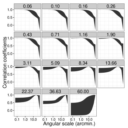
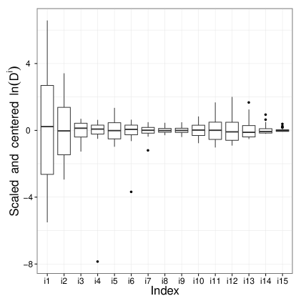
In Figure 2 we show the full range of values in covariance diagonal components (left) and correlation coefficients (right) over the design space. The diagonal terms of the covariance span well over an order of magnitude in value and differ in shape as the angular projection of the one-halo term changes. The amount of cross-correlation is mostly stable with cosmology however, it does vary greatly at large scales. Figure 3 shows the amount of variation in the GCD compoments, $\mathbf{d}$ and $\bm{\phi}$ over the full simulated space. In this decomposition we see much of the variation in the covariance has been confined to fewer components.

4.2 Basis functions

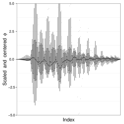
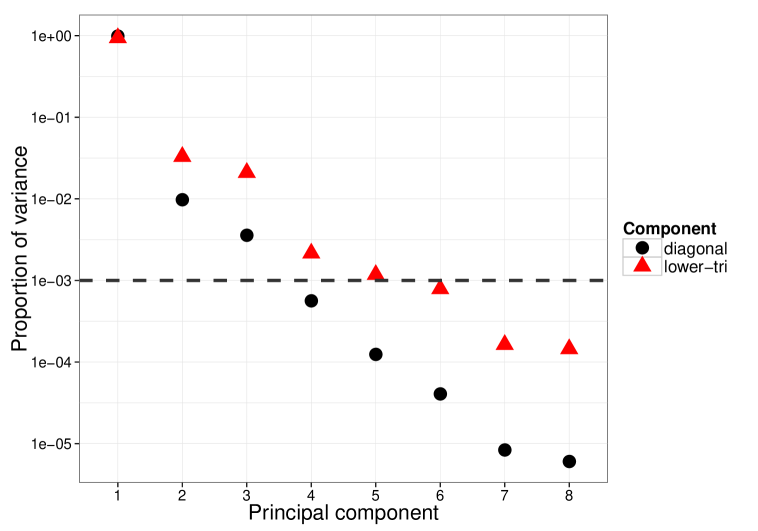
In Figure 4 we show the first 8 PCA amplitudes as a function of mode index. For both the diagonal elements $\mathbf{d}$ and lower triangular elements $\bm{\phi}$ we see that most of the variation is contained within the first few modes of the decomposition allowing for significant reduction in the dimensionality of the covariance matrices over the full simulation design. We retain those PC modes that contribute at least $10^{-3}$ to the fractional variance.

4.3 Parameters of the Gaussian Process

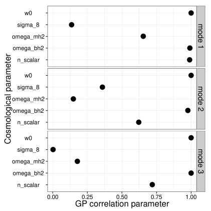
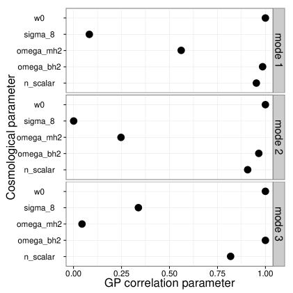
As stated previously in Section 3.4 the amount of correlation in the GP modes informs us how strongly dependent the information in the CDC is on different cosmological parameters. Figure 5 shows the mode amplitude correlations (i.e. the $\rho_{X}$ parameters in Eq. 3.10) with each cosmological parameter in a ‘sensitivity’ analysis. A value of one means that the mode amplitudes are highly correlated along a given parameter axis, so the emulator is not sensitive to variations in this parameter. This also means sparser sampling of simulation design runs can be used. The parameters $w_{0}$, $\Omega_{b}h^{2}$, and $n_{s}$ are often the most correlated, indicating they have little impact on the covariance. The mode amplitudes are consistently weakly correlated along the $\sigma_{8}$ and $\Omega_{m}h^{2}$ parameter axes, indicating these parameters largely determine the form of the covariance as might be expected because the amplitude of the shear correlation function depends on the product $\sim\sigma_{8}^{2}\Omega_{m}^{0.6}$

4.4 Mode amplitudes of the covariance matrices

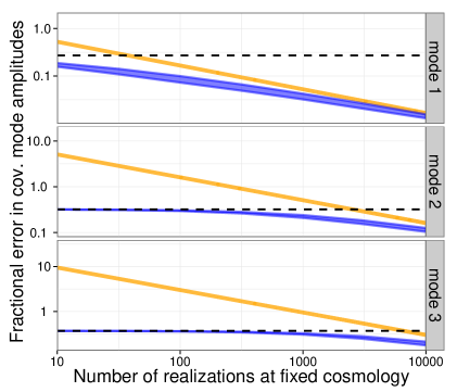
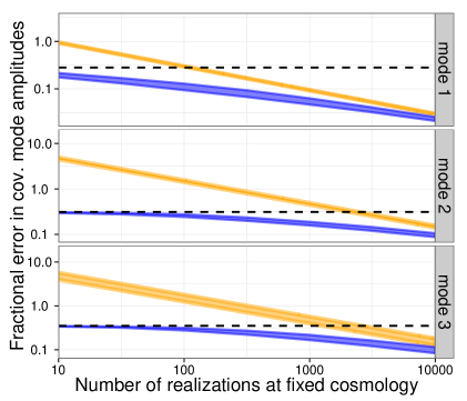
The marginal Fisher errors of the mode amplitudes for the diaginal and lower triagular compoments of the GCD, $\gamma$ and $\delta$ respectively, are shown in Figure 6 as functions of $n_{r}$ for $n_{d}=32$. Here we compare the emulator error performance in the mode amplitudes to that of a brute force simulation. The errors shown are for a single cosmology design point, however the emulator is constrained over the full parameter space considered. We see that the emulator performs as well or better depending on the number of simulation run and with the added benefit of modeling the CDC over the full parameter space. While the fractional error at higher modes is constrained by the GP prior, keep in mind that the prior is informed from the data. The GP prior can be thought of as the maximum variation over all the cosmology design points.

If we compare the two lines in Fig. 6 for fixed fractional error (i.e. reading horizontally), we see that in many cases the number of simulations required for the emulator is about one order of magnitude smaller. The results for other $n_{d}$ values are similar, except that the GP prior is less significant for a fixed $n_{r}$.

We have not propagated any uncertainties from the calibration of the GP parameters or the truncation of the PC basis expansion. Including these uncertainties will tend to bring the emulator forecasts closer to those assuming no relationship between modes at different design points. But, given the success of other emulator frameworks in the literature, we do not expect additional sources of uncertainty to qualitatively change the results in Fig. 6.

Figure 6: Forecasted errors on the mode amplitudes of the diagonal (left) and lower-triangular (right) components in the GCD of the covariance matrices. The panels show the first 3 principle components in each case. The blue bands show the range of marginal errors over 32 design points when using all design points simultaneously to constrain the mode amplitudes. The orange bands show the range of marginal errors when the simulations run with different cosmologies are used The errors then scale with $\sqrt{n_{r}}$. The dashed horizontal line indicates the variance in the GP prior imposed on each mode amplitude (where the GP prior parameters are determined by maximum-likelihood estimates given the model covariance matrices at each design point).

5 Conclusions

Estimating covariance matrices of power-spectra and correlation functions is a computationally intensive task that requires many CPU hours of simulations to achieve the accuracy required for future surveys [18, 19]. In this paper we have shown that the precision in the estimated cosmology dependent covariance matrices can only improve as fast as $1/\sqrt{n_{r}}$, where $n_{r}$ is the number of simulation realizations, if one considers each cosmological model independently. If however, one simultaneously models the simulations at different cosmologies using Gaussian Processes, the number of simulations required to reach a given precision can be reduced while also modeling the CDC (which cannot otherwise be done with a sample of disjoint cosmological simulations). This makes the computational challenges of simulating the analysis much more tractable. However, we do not find orders of magnitude improvements in the number of simulations needed and other methods of estimating the covariances should be considered in combination with the emulator presented here (e.g. shrinkage estimators [20], large-scale mode-resampling [21], and optimized simulation design spaces [10].)

Future work will demonstrate the accuracy of the full emulator framework, with all uncertainties propagated including those from the lack of sample covariance estimators at each design point.

Appendix A The halo model

For our ‘simulation’ of covariances we employ the halo model [17] to estimate the nonlinear matter power spectrum to be used in the analysis. This modeling is part of the python cosmology prediction package CHOMP. We use the halo model as defined in [22] using a [23] mass function. This model is accurate to within 20% at 1 arcminute when compared to $N$-body simulations from [24] and within 10% between 20-200 arcminutes. For the covariances we follow the formalism of several papers [25, 26, 27], considering two contributions to our covariance matrix, a Gaussian and a non-Gaussian term.

$$C(\theta_{1},\theta_{2})=C_{G}(\theta_{1},\theta_{2})+C_{NG}(\theta_{i},\theta_{j})$$ (A.1)

For the Gaussian term we use the definitions as laid out in [26] using Limber’s approximation

$$C_{G}^{ijkl}(\theta_{1},\theta_{2})=\frac{1}{2\pi A}\int ldlJ_{0}(l\theta_{i})J_{0}(l\theta_{j})\{P^{ik}(l)P^{jl}(l)+P^{il}(l)P^{jk}(l)\ +\frac{\sigma^{4}}{4\bar{n}^{i}\bar{n}^{j}}(\delta_{ik}\delta_{jl}+\delta_{il}\delta_{jk})\}$$ (A.2)

where $A$ is the area of the survey, $\sigma^{2}$ is the variance per galaxy pair, $\bar{n}^{i}$ is the density of galaxies for probe $i$, and $P^{ij}(l)$ is the projected power spectrum written as

$$P^{ij}(l)=\int_{0}^{\chi_{H}}d\chi\frac{f^{i}(\chi)f^{j}(\chi)}{\chi^{-2}}P(\frac{l}{\chi}:\chi)$$ (A.3)

where $P$ is the non-linear matter power spectrum as a function of redshift, $\chi$ is the comving distance, $f^{i}(\chi)$ is the weighted window function (e.g. the lensing kernel), and the integration is from 0 to the horizon.

For the non-Guassian term, we model only the one halo term of the halo-trispectrum. Following [28], this term is

$$T_{1-halo}(k_{1},k_{2})=\int dM\frac{dn}{dM}(\frac{M}{\bar{\rho}})^{4}*y(k_{1},M)^{2}*y(k_{2},M)^{2}$$ (A.4)

Where $\frac{dn}{dM}$ iwthe number density of halos as a fucntion of mass $M$, $\bar{\rho}$ is the matter density, and $y$ is the Fourier transform of halo density profile normalized to 1 at $k=0$. For this analysis we assume that halos follow an NFW [29] profile. Here we only considering the tri-spectrum in a parallelogram configuration as required by the covariance estimation. Projecting this configuration with the window functions we have

$$\mathcal{T}^{ijkl}(l_{1},l_{2})=\int_{0}^{\chi_{H}}f^{i}(\chi)f^{j}(\chi)f^{k}(\chi)f^{l}(\chi)/\chi^{-6}T(\frac{l_{1}}{\chi},\frac{l_{2}}{\chi}:\chi)$$ (A.5)

The final form of the non-Gaussian covaraince is

$$C^{ijkl}(\theta_{1},\theta_{2})=\frac{1}{4\pi^{2}A}\int l_{1}dl_{1}\int l_{2}dl_{2}J_{0}(l_{1}\theta_{1})J_{0}(l_{2}\theta_{2})\mathcal{T}^{ijkl}(l_{1},l_{2})$$ (A.6)

It is worth noting that more terms contribute to the covariance and are highly dependent on the specified survey geometry. One parameterization as presented by [30] gives the beat coupling and halo sample variance as a single Super-Sample Covariance term. This term is as dominant as the non-Gaussian term at scales $k>1$ Mpc/h, however, we do not consider them in this analaysis currently. While this term is not sub-dominant, within the scope of this paper, we do not expect it to significantly change the covariance’s dependence on cosmology or add any challenge to the marix decomposition and emulation presented in this work.

Figure 7: Comparison of CHOMP lensing two-point functions with those from [31], and [24] using ray-tracing through $N$-body simulations. Left: Comparison between the simulations and the $chomp$ shear correlations. Right: Comparison bewteen the simiulated and predicted covariance matrices. The correlation function is predicted to within 10% at acminute scales in the halo model and to sub-arcminute scales for HaloFit. The covariances agree to within 20% for scales larger than 10 arcminutes. The results of this anlaysis hold as long as the variation of both the simulated and predicted covariances are smooth as a function of cosmology.

Appendix B Validation of halo model shear correlation covariance

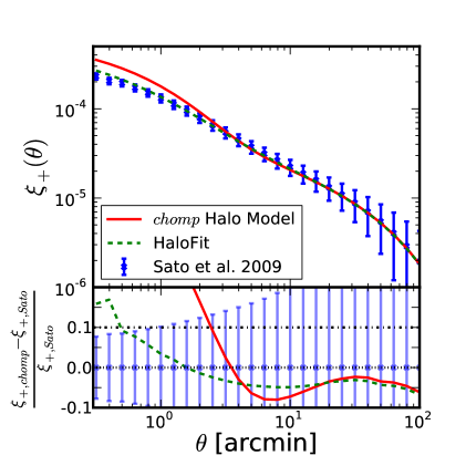
To apply our forecasts for planning simulation runs, it is important to understand how well our covariance model may reproduce the covariance derived from simulations. In this section we compare our covariance model from the CHOMP code to the 1000 lensing simulation realizations from [31, 24]. These simulations give the power spectra and real-space correlations of cosmic shear for a variety of source redshifts. We compare our model constructed from the CHOMP cosmology package to these sims. The left pannel of Figure 7 shows the level of agreement between our models and the Sato results. We see good agreement between these models and the $N$-body sims. For the halofit model derived in [32] we find agreement to within 5% at arcminute scales for the real-space correlation. The Halo Model used in this analysis fare’s slighly worse but is still within 10% for similar scales to the HaloFit model.

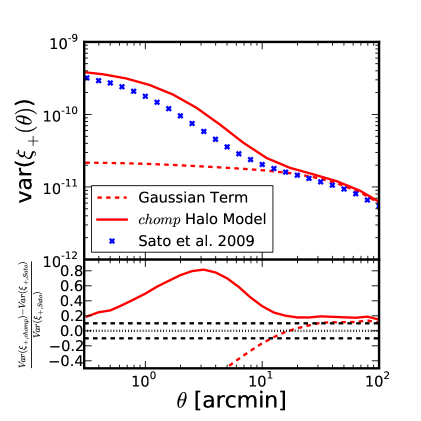
The right pannel of Figure 7 shows how well the halo model recovers the features of the Sato covarianes. Overall, we find agreement between the simluations at various scales. The reader should keep in mind, though, that the results of this paper hold as long as the covariance matrix variation with respect to cosmology is smooth and therefore still gives an adiquate description of the covariance as a funciton of cosmology. Future work will explore the robustness and limitations of this code further.

References

- [1] S. Dodelson and M. D. Schneider, Simulation Covariance Error, arXiv.org (Apr., 2013) [arXiv:1304.2593].
- [2] T. Eifler, P. Schneider, and J. Hartlap, Dependence of cosmic shear covariances on cosmology. Impact on parameter estimation, A&A 502 (Aug., 2009) 721–731, [arXiv:0810.4254].
- [3] M. J. Jee, J. A. Tyson, M. D. Schneider, D. Wittman, S. Schmidt, and S. Hilbert, Cosmic Shear Results from the Deep Lens Survey. I. Joint Constraints on M and 8 with a Two-dimensional Analysis, ApJ 765 (Mar., 2013) 74, [arXiv:1210.2732].
- [4] P. Norberg, C. M. Baugh, E. Gaztañaga, and D. J. Croton, Statistical analysis of galaxy surveys - I. Robust error estimation for two-point clustering statistics, MNRAS 396 (June, 2009) 19–38, [arXiv:0810.1885].
- [5] E. Lawrence, K. Heitmann, M. White, D. Higdon, C. Wagner, S. Habib, and B. Williams, The Coyote Universe. III. Simulation Suite and Precision Emulator for the Nonlinear Matter Power Spectrum, ApJ 713 (Apr., 2010) 1322–1331, [arXiv:0912.4490].
- [6] R. G. Bower, I. Vernon, M. Goldstein, A. J. Benson, C. G. Lacey, C. M. Baugh, S. Cole, and C. S. Frenk, The parameter space of galaxy formation, MNRAS 407 (Oct., 2010) 2017–2045, [arXiv:1004.0711].
- [7] Y. Lu, H. J. Mo, M. D. Weinberg, and N. Katz, A Bayesian approach to the semi-analytic model of galaxy formation: methodology, MNRAS 416 (Sept., 2011) 1949–1964, [arXiv:1004.2518].
- [8] Y. Lu, H. J. Mo, N. Katz, and M. D. Weinberg, Bayesian inference of galaxy formation from the K-band luminosity function of galaxies: tensions between theory and observation, MNRAS 421 (Apr., 2012) 1779–1796, [arXiv:1109.6658].
- [9] F. A. Gómez, C. E. Coleman-Smith, B. W. O’Shea, J. Tumlinson, and R. L. Wolpert, Characterizing the Formation History of Milky Way like Stellar Halos with Model Emulators, ApJ 760 (Dec., 2012) 112, [arXiv:1209.2142].
- [10] M. D. Schneider, Ó. Holm, and L. Knox, Intelligent Design: On the Emulation of Cosmological Simulations, ApJ 728 (Feb., 2011) 137–+, [arXiv:1002.1752].
- [11] M. D. Schneider, L. Knox, S. Habib, K. Heitmann, D. Higdon, and C. Nakhleh, Simulations and cosmological inference: A statistical model for power spectra means and covariances, Phys. Rev. D 78 (Sept., 2008) 063529–+, [arXiv:0806.1487].
- [12] M. Pourahmadi, M. J. Daniels, and T. Park, Simultaneous modelling of the Cholesky decomposition of several covariance matrices, Journal of Multivariate Analysis 98 (2007), no. 3 568–587.
- [13] M. J. Daniels and M. Pourahmadi, Bayesian analysis of covariance matrices and dynamic models for longitudinal data, Biometrika 89 no. 3 553–566.
- [14] M. Pourahmadi, Covariance Estimation: The GLM and Regularization Perspectives, Statistical Science 26 (Aug., 2011) 369–387.
- [15] S. Habib, K. Heitmann, D. Higdon, C. Nakhleh, and B. Williams, Cosmic calibration: Constraints from the matter power spectrum and the cosmic microwave background, Phys. Rev. D 76 (Oct., 2007) 083503, [astro-ph/0702348].
- [16] C. E. Rasmussen and C. K. I. Williams, Gaussian Processes for Machine Learning. The MIT Press, 2006.
- [17] A. Cooray and R. Sheth, Halo models of large scale structure, Phys. Rep. 372 (Dec., 2002) 1–129, [astro-ph/0206508].
- [18] LSST Science Collaboration, P. A. Abell, J. Allison, S. F. Anderson, J. R. Andrew, J. R. P. Angel, L. Armus, D. Arnett, S. J. Asztalos, T. S. Axelrod, and et al., LSST Science Book, Version 2.0, ArXiv e-prints (Dec., 2009) [arXiv:0912.0201].
- [19] J. Amiaux, R. Scaramella, Y. Mellier, B. Altieri, C. Burigana, A. Da Silva, P. Gomez, J. Hoar, R. Laureijs, E. Maiorano, D. Magalhães Oliveira, F. Renk, G. Saavedra Criado, I. Tereno, J. L. Auguères, J. Brinchmann, M. Cropper, L. Duvet, A. Ealet, P. Franzetti, B. Garilli, P. Gondoin, L. Guzzo, H. Hoekstra, R. Holmes, K. Jahnke, T. Kitching, M. Meneghetti, W. Percival, and S. Warren, Euclid mission: building of a reference survey, in Society of Photo-Optical Instrumentation Engineers (SPIE) Conference Series, vol. 8442 of Society of Photo-Optical Instrumentation Engineers (SPIE) Conference Series, Sept., 2012. arXiv:1209.2228.
- [20] A. C. Pope and I. Szapudi, Shrinkage estimation of the power spectrum covariance matrix, MNRAS 389 (Sept., 2008) 766–774, [arXiv:0711.2509].
- [21] M. D. Schneider, S. Cole, C. S. Frenk, and I. Szapudi, Fast Generation of Ensembles of Cosmological N-body Simulations Via Mode Resampling, ApJ 737 (Aug., 2011) 11, [arXiv:1103.2767].
- [22] U. Seljak, Analytic model for galaxy and dark matter clustering, MNRAS 318 (Oct., 2000) 203–213, [astro-ph/0001493].
- [23] R. K. Sheth and G. Tormen, Large-scale bias and the peak background split, Monthly Notices of the Royal Astronomical Society 308 (Sep, 1999) 119–126, [astro-ph/9901122].
- [24] M. Sato, M. Takada, T. Hamana, and T. Matsubara, Simulations of wide-field weak-lensing surveys. ii. covariance matrix of real-space correlation functions, The Astrophysical Journal 734 (Jun, 2011) 76, [arXiv:1009.2558].
- [25] R. Scranton, Testing the halo model against the sdss photometric survey, Monthly Notices of the Royal Astronomical Society 339 (Feb, 2003) 410–426, [astro-ph/0205517].
- [26] B. Joachimi, P. Schneider, and T. Eifler, Analysis of two-point statistics of cosmic shear, Astronomy and Astrophysics 477 (Jan, 2008) 43–54, [arXiv:0708.0387].
- [27] M. Takada and B. Jain, The impact of non-Gaussian errors on weak lensing surveys, MNRAS 395 (June, 2009) 2065–2086, [arXiv:0810.4170].
- [28] A. Cooray and W. Hu, Power Spectrum Covariance of Weak Gravitational Lensing, ApJ 554 (June, 2001) 56–66, [astro-ph/0012087].
- [29] J. F. Navarro, C. S. Frenk, and S. D. M. White, A Universal Density Profile from Hierarchical Clustering, ApJ 490 (Dec., 1997) 493, [astro-ph/9611107].
- [30] M. Takada and W. Hu, Power Spectrum Super-Sample Covariance, ArXiv e-prints (Feb., 2013) [arXiv:1302.6994].
- [31] M. Sato, T. Hamana, R. Takahashi, M. Takada, N. Yoshida, T. Matsubara, and N. Sugiyama, Simulations of Wide-Field Weak Lensing Surveys. I. Basic Statistics and Non-Gaussian Effects, ApJ 701 (Aug., 2009) 945–954, [arXiv:0906.2237].
- [32] R. Takahashi, M. Sato, T. Nishimichi, A. Taruya, and M. Oguri, Revising the Halofit Model for the Nonlinear Matter Power Spectrum, ApJ 761 (Dec., 2012) 152, [arXiv:1208.2701].