Quantum Corrections to the Polarizability and Dephasing in Isolated Disordered Metals

Abstract

We study the quantum corrections to the polarizability of isolated metallic mesoscopic systems using the loop-expansion in diffusive propagators. We show that the difference between connected (grand-canonical ensemble) and isolated (canonical ensemble) systems appears only in subleading terms of the expansion, and can be neglected if the frequency of the external field, $\,\omega$, is of the order of (or even slightly smaller than) the mean level spacing, $\,\Delta$. If $\,\omega\ll\Delta$, the two-loop correction becomes important. We calculate it by systematically evaluating the ballistic parts (the Hikami boxes) of the corresponding diagrams and exploiting electroneutrality. Our theory allows one to take into account a finite dephasing rate, $\,\gamma$, generated by electron interactions, and it is complementary to the nonperturbative results obtained from a combination of random matrix theory (RMT) and the $\,\sigma$-model, valid at $\gamma\to 0$. Remarkably, we find that the two-loop result for isolated systems with moderately weak dephasing, $\gamma\sim\Delta$, is similar to the result of the RMT+$\sigma$-model even in the limit $\omega\to 0$. For smaller $\gamma$, we discuss the possibility to interpolate between the perturbative and the nonperturbative results. We compare our results for the temperature dependence of the polarizability of isolated rings to the experimental data of R. Deblock et al. [Phys. Rev. Lett.  84, 5379 (2000); Phys. Rev. B 65, 075301 (2002)], and we argue that the elusive 0D regime of dephasing might have manifested itself in the observed magneto-oscillations. Besides, we thoroughly discuss possible future measurements of the polarizability, which could aim to reveal the existence of 0D dephasing and the role of the Pauli blocking at small temperatures.

I Introduction

Interference phenomena in mesoscopic electronic systems require phase coherence, which is cut beyond the so-called dephasing time $\,\tau_{\phi}$. At low temperatures $T\lesssim 1K$, where phonons are frozen out, dephasing is caused mainly by electron interactions, which lead to a finite dephasing rate Altshuler_Disordered_1985 $\,\gamma\equiv 1/\tau_{\phi}$. In large systems with a small Thouless energy, $E_{\rm Th}\ll T$, dephasing crucially depends on dimensionality and geometryAltshuler_SmallEnergyTransfers_1982 . However, if the system is finite and $T\lesssim E_{\rm Th}$, spatial coordinates become unimportant and a 0D regime of rather weak dephasing is expected to occur Sivan_QuasiParticleLifetime_1994 . This regime is characterized by a universal temperature dependence of the dephasing rate, $\gamma_{\rm 0D}\sim\Delta T^{2}/E_{\rm Th}^{2}$, where $\,\Delta\,$ is the mean-level spacing. This $T$-dependence of $\gamma$ can be explained by simple power counting: Pauli blocking restricts the number of available final scattering states of the electrons, therefore both the energy transfer and the available phase-space are $\,\propto T$, similar to the standard result for a clean Fermi-liquid. However, despite the fundamental nature and the physical importance of 0D dephasing, attempts to observe it experimentally in mesoscopic systems have been unsuccessful so far.

In transport experiments, the 0D regime is generally difficult to observe, since quantum transport is almost insensitive to $\gamma$ at $T\ll E_{\rm Th}$. For example, the weak localization correction to the classical dc conductivity is cut mainly by the dwell time, $\,\tau_{\rm dw}\ll 1/\gamma_{\rm 0D}$, see LABEL:Treiber_QuantumDot_2012 for a detailed discussion. This is an unavoidable problem which occurs in any open system even if the coupling to leads is weak.

In this work, we concentrate on interference phenomena in isolated systems, where $\,\tau_{\rm dw}\to\infty\,$ and where 0D dephasing is not masked by the coupling to the environment. Deeply in the 0D regime at $\,\gamma\ll\Delta\,$, the spectrum of the isolated system is discrete Altshuler_QuasiParticleLifetime_1997 ; Blanter_ScatteringRate_1996 and, in the absence of other mechanisms of dephasing, random matrix theory (RMT) can be used as a starting point for an effective low-energy theory at $\,E\ll E_{\rm Th}$ Kravtsov_Corrections_1994 ; Blanter_Polarizability_1998 . Unfortunately, RMT is not appropriate for a systematic account of dephasing.

If one is interested in the (almost 0D) regime $\,\gamma\leq\Delta$, where the spectrum is not yet discrete, the usual mesoscopic perturbation theory Montambaux_Book_2007 can be used, which is able to take into account dephasing in all regimes. However, the description of quantum effects in isolated systems provides a further technical challenge. Namely, the usual perturbation theory is well developed for a fixed chemical potential $\mu$; i.e. it describes systems in the grand-canonical ensemble (GCE). Realizing the canonical ensemble (CE), where the number of particles is fixed instead, can be rather tricky, see, e.g., LABEL:Kamenev_StatEnsemble_1993. In the following, we assume that a description in terms of the so-called Fermi-level pinning ensemble introduced in Ref. [Lehle_Canonical_1995, ] and [Altland_Canonical_1992, ] is applicable remark_canonical .

The dephasing rate of an isolated mesoscopic system can be explored, for instance, by measuring quantum components of the electrical polarizability $\alpha$ at a given frequency $\,\omega$:

$$\alpha(\omega)={\bf{d}}(\omega)\cdot{\bf{E}}(\omega)/|{\bf{E}}(\omega)|^{2}\,.$$ (1)

Here $\,{\bf{E}}\,$ is a spatially homogeneous electric field and $\,{\bf{d}}\,$ is the total induced dipole moment in the sample.

Gorkov and Eliashberg studied the polarizability in the seminal work LABEL:Gorkov_Eliashberg_1965 by using results from RMT and found very large quantum corrections. Later, it was shown in LABEL:Rice_Polarizability_1973 that the corrections are significantly reduced if screening is taken into account correctly Blanter_GorkovEliashberg_1996 . Efetov reconsidered Gorkov and Eliashberg’s calculation in LABEL:Efetov_Polarizability_1996 and derived a formula which accounts for screening in the random phase approximation (RPA) and expresses the quantum corrections to $\alpha$ in terms of correlation functions of the wave-functions and energy levels of the system. Noat et al. Noat_Polarizability_1996 used a simple model supported by numerical simulations to analyze the difference between the GCE and the CE, and established that the quantum corrections are always small for systems with a large dimensionless conductance. Subsequently, Mirlin and Blanter Blanter_Polarizability_1998 studied the polarizability using a combination of RMT and the diffusive $\sigma$-model. In particular, they have calculated $\omega$-dependence of $\alpha$ at $\omega\ll E_{\rm Th}$ for the case of the CE at $\,\gamma=0$. Thus, neither the temperature nor the magnetic field dependence of $\,\alpha\,$ has been described until now.

Besides the progress made in theory, experimental measurements of the quantum corrections have been reported in Ref. [Deblock_Experiment_2000, ] and [Deblock_Experiment_2002, ]. The authors measured the $\,T$-dependence of the polarizability of small metallic rings placed in a superconducting resonator (with a fixed frequency $\omega$) in a perpendicular magnetic field and tried to extract the $\,T$-dependence of $\,\tau_{\phi}\,$ by using an empirical fitting equation. A fingerprint of 0D dephasing was found at low temperatures, though a reliable identification of the temperature dependence of $\tau_{\varphi}$ calls for a more rigorous theory.

Motivated by the experimental results, we develop a perturbative theory for the quantum corrections $\Delta\alpha$ to the polarizability by using the mesoscopic “loop-expansion” in diffusons and Cooperons, where $\,\gamma\,$ plays the role of a Cooperon mass. We have chosen the experimentally relevant parameter range $\,\max(\omega,\gamma)\gtrsim\Delta\,$. Generically, the difference between the GCE and the CE can be important up to energies substantially exceeding $\,\Delta$, see the discussions in LABEL:Kamenev_StatEnsemble_1993. To check whether this statement also applies for $\,\Delta\alpha$, we calculate leading and subleading corrections in the Fermi-level pinning ensemble. The former corresponds solely to the one-loop answer of the GCE while the latter includes the two-loop answer of the GCE and additional terms generated by fixing the number of particles in the CE. We show that, within our approach, the leading term of the perturbative expansion for $\,\Delta\alpha\,$ suffices for its theoretical description in the experimentally relevant parameter range of Ref. [Deblock_Experiment_2000, ] and [Deblock_Experiment_2002, ]. This important result of the present paper allows us to find the dependence of $\,\Delta\alpha\,$ on temperature and on magnetic field. Our theoretical results are in good qualitative agreement with the experiments, though we show that the present experimental data are not sufficient for a reliable identification of 0D dephasing. We suggest repeating the experimental measurements with higher precision and lower frequencies and using the fitting procedures which we propose in the present paper. We have good hopes that the elusive 0D regime of dephasing may be detectable in this manner in the near future.

The rest of this paper is organized as follows:

Section II: we derive a general expression for the polarizabiliy as a functional of the density response function in the RPA.

Section III: we calculate the leading quantum corrections of the density response function for connected as well as isolated disordered metals. This part of the paper is rather formal and technical. Readers who are not interested in details of the calculations can safely skip it, paying attention only to our key results, which we list here. First, we derive the one- and two-loop quantum corrections for the GCE which are presented in Eqs. (17,18) of Subsection III.1. A “naive” loop-expansion for the GCE suffers from a double-counting problem of some diagrams which leads to a violation of the particle conservation law (electroneutrality) accompanied by artificial UV divergences. We suggest an algorithm of constructing the diagrams which allows one to avoid all these problems. Our method can be straightforwardly checked for the one-loop calculations, see Fig. 2, and we extend it to the much more cumbersome two-loop diagrams shown in Fig. 3. Second, we calculate the leading diagrams which appear due to fixing the Fermi level in the CE. Their contribution is given by Eq. (24) of Subsection III.2.

Section IV: we use the results from Section III to derive a general equation for the quantum corrections $\Delta\alpha$.

Section V: we compare our findings to the results obtained from a combination of the RMT and the $\sigma$-model. We show that the diagrammatic result in the limit of a large conductance, Eq. (30), qualitatively reproduces all features of the nonperturbative answers for almost 0D systems at $\,0\leq\omega<E_{\rm Th}$, see Fig. 7.

Section VI: we apply our results for $\Delta\alpha$ to the ring geometry, present a comparison with previous experiments and discuss possible future measurements which can reliably confirm the existence of 0D dephasing.

II Polarizability

The polarizability (1) is governed by the induced dipole moment in the sample,

$${\bf{d}}(\omega)=\int_{V}\!{\rm d}^{3}{\bf{x}}\,\left[{\bf{x}}\cdot n_{\rm ind}({\bf{x}},\omega)\right]\,,$$ (2)

where $n_{\rm ind}$ is the induced charge density. In the case of a good metal, screening should be taken into account in the random phase approximation (RPA), which results in the following expressions for the Fourier transform of $n_{\rm ind}$:Bruus_Book_2004

$$n_{\rm ind}({\bf{q}},\omega)=-2e^{2}\frac{\chi({\bf{q}},\omega)}{\epsilon({\bf{q}},\omega)}\phi_{\rm ext}({\bf{q}},\omega)\,.$$ (3)

Here $\phi_{\rm ext}({\bf{x}},\omega)=-{\bf{E}}(\omega)\cdot{\bf{x}}$ is the external electric potential, $\epsilon({\bf{q}},\omega)=1-2U({\bf{q}})\chi({\bf{q}},\omega)$ is the dielectric function, $U$ is the bare Coulomb potential, and $\chi$ is the density response function per spin. By using the Kubo formula, $\chi$ can be expressed in terms of the commutator of the density operators $\,\hat{n}$:

$$\chi({\bf{q}},\omega)=i\int_{V}\!{\rm d}^{3}{\bf{x}}\,\ \int_{0}^{\infty}\!\!\!\!{\rm d}t\,\,\langle\left[\hat{n}({\bf{x}},t),\hat{n}({\bf{0}},0)\right]\rangle e^{-i({\bf{q}}{\bf{x}}-\omega t)}\,.$$ (4)

We assume spatial homogeneity of the system, which is restored after disorder averaging.

Inserting Eqs. (2,3) in Eq. (1), we find the following expression for the polarizability:

$$\alpha(\omega)\!=\!\frac{2e^{2}}{|{\bf{E}}(\omega)|^{2}}\frac{1}{V}\sum_{{\bf{q}}\neq{\bf{0}}}\ \phi_{\rm ext}({\bf{q}},\omega)\frac{\chi({\bf{q}},\omega)}{\epsilon({\bf{q}},\omega)}\phi_{\rm ext}(-{\bf{q}},\omega)\ \,.$$ (5)

Note that the zero-mode does not contribute to $\alpha$ because of electroneutrality of the sample:

$$\chi({\bf{q}}\equiv{\bf{0}},\omega)=0\,.$$ (6)

For a clean metal at $\omega\ll{v_{\rm F}}{\bf{q}}$ (${v_{\rm F}}\,$ is the Fermi velocity), $\chi$ is local and is given by the density of states at the Fermi level:

$$\chi({\bf{q}},\omega\to 0)=\rho_{0}\,.$$ (7)

The same equation holds true for a disordered (classical) metal at $\omega\ll D{\bf{q}}^{2}$ ($D\,$ is the diffusion constant), see Section III. Eqs.(5,7) yield the ”classical“ polarizability $\alpha_{0}$ of the disordered sample.

III Density response function

In this section, we consider the density response function of the disordered metal which is needed to calculate the polarizability, Eq. (5). We will start with the loop-expansion of the disorder-averaged $\,\chi\,$ in the GCE: $\,\overline{\chi}|_{\mu={\rm const}}\equiv\overline{\chi}_{\mu}$. It is relevant for the polarizability of the connected system. Besides, the two-loop contribution to $\,\overline{\chi}_{\mu}\,$ is needed to study the difference between the answers in the GCE and the CE. The latter is described in the second part of the present section.

We consider only weakly-interacting disordered systems at small temperatures. The main role of the electron interaction is to generate a finite $\,T$-dependent dephasing rate for Cooperons. Therefore, we derive the density response function for the non-interacting system at $\,T=0\,$ and take into account $\,\gamma(T)\,$ at the end of the calculations.

III.1 Grand canonical ensemble

Simplifying Eq. (4) for the non-interacting system at $T=0$ and fixed $\,\mu$, $\,\chi_{\mu}\,$ can be presented in terms of retarded/advanced ($G^{R/A}$) Green’s functions (GFs) Montambaux_Book_2007 :

$$\chi_{\mu}({\bf{x}},{\bf{y}},\omega)=-\int_{-\infty}^{0}\!{\rm d}\epsilon\,$$ (8)

$$\times\bigg{(}\rho_{\mu+\epsilon}({\bf{x}},{\bf{y}})G^{A}_{\mu+\epsilon-\omega}({\bf{y}},{\bf{x}})+G^{R}_{\mu+\epsilon+\omega}({\bf{x}},{\bf{y}})\rho_{\mu+\epsilon}({\bf{y}},{\bf{x}})\bigg{)}\,.$$

Here we have introduced the spectral function (or the non-local density of states):

$$\rho_{\epsilon}({\bf{x}},{\bf{y}}) \equiv\frac{i}{2\pi}\left[G_{\epsilon}^{R}({\bf{x}},{\bf{y}})-G_{\epsilon}^{A}({\bf{x}},{\bf{y}})\right]\,.$$ (9)

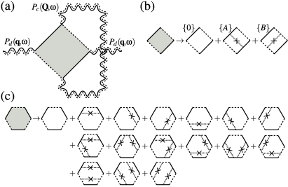
Figure 1: (a): One-loop correction to the density response function in the GCE. Retarded (advanced) GFs are denoted by solid (dashed) lines. Impurity lines, corresponding to the correlation function (10), are denoted by dotted crossed lines. Diffusive propagators are represented by wavy double lines. They denote impurity ladders between the corresponding GFs of opposite retardation either in the particle-particle (Cooperon, $P_{c}$) or in the particle-hole (diffuson, $P_{d}$) channel. (b) and (c): Dressed 4- and 6-point Hikami boxes which include diagrams with one or two additional impurity lines connecting GFs of the same retardation.

In the presence of a random Gaussian white-noise disorder potential $V({\bf{x}})$ with correlation function

$$\overline{V({\bf{x}})V({\bf{y}})}=\frac{1}{2\pi\rho_{0}\tau}\delta({\bf{x}}-{\bf{y}})\,,$$ (10)

the disorder-averaged GFs are given by

$$\overline{G}^{R/A}_{\epsilon}({\bf{k}})=\frac{1}{\epsilon-\epsilon_{\bf{k}}\pm i/2\tau},$$ (11)

where $\tau$ is the impurity scattering time and $\,\epsilon_{\bf{k}}\,$ is the particle dispersion relation.

The disorder average of Eq. (8) can be calculated with the help of the usual diagrammatic methods,Altshuler_Disordered_1985 which yield the loop-expansion:

$$\overline{\chi}_{\mu}({\bf{q}},\omega)=\chi_{0}({\bf{q}},\omega)+\sum_{j}\delta\chi_{\rm GCE}^{(j)}\,.$$ (12)

Here $\,j\,$ is the number of loops built from impurity ladder diagrams which include ladders in the particle-hole channel (diffuson propagators) or in the particle-particle channel (Cooperon propagators). The leading (classical) term is well-knownAltshuler_Disordered_1985 :

$$\chi_{0}({\bf{q}},\omega)= \ \rho_{0}\frac{D{\bf{q}}^{2}}{D{\bf{q}}^{2}-i\omega}\,.$$ (13)

It obeys the fundamental requirement of electroneutrality, Eq. (6), and reduces to Eq. (7) at $\omega\ll D{\bf{q}}^{2}$.

The leading quantum correction $\,\delta\chi_{\rm GCE}^{(1)}\,$ describes the weak-localization correction to the diffusion constant Vollhardt_Localization_1980 and, therefore, is also well-known. Nevertheless, we would like to recall the basic steps of its derivation, which will be important to find the more complicated subleading term $\delta\chi_{\rm GCE}^{(2)}$.

The one-loop diagram, which yields $\,\delta\chi_{\rm GCE}^{(1)}$, is shown in Fig. 1(a). It includes two diffuson propagators $P_{d}$ and one Cooperon propagator $P_{c}$, which are given by

$$P_{d}({\bf{q}},\omega)=\frac{1}{D{\bf{q}}^{2}-i\omega}\,,\quad P_{c}({\bf{Q}},\omega)=\frac{1}{D{\bf{Q}}^{2}-i\omega+\gamma}\,.$$ (14)

The (ballistic) part of the diagram which connects the diffusive propagators is known as a 4-point Hikami box Hikami_AndersonLocalization_1981 . It consists of three diagrams of the same order in $({\epsilon_{\rm F}}\tau)^{-1}$ shown in Fig. 1(b) and labeled by $\{0\}$, $\{A\}$, and $\{B\}$, which are obtained by inserting additional impurity lines between GFs of the same retardation (“dressing” the Hikami box). The Hikami box should be calculated by expanding the GFs in each of the three diagrams in the transferred momenta and energies. A direct summation of the three diagrams gives

$$H_{4}^{\rm(direct\ sum)}=4\pi\rho_{0}\tau^{4}\left[D{\bf{q}}^{2}+D{\bf{Q}}^{2}-i\omega\right]\,.$$ (15)

The second and third terms in parentheses are manifestly incorrect as they violate electroneutrality, Eq. (6), and lead to an unphysical UV divergence in $\,\delta\chi_{\rm GCE}^{(1)}$. The incorrect terms originate from a double-counting problem: the diagram with a single impurity line, which contributes (via the diffuson) to the classical result of Eq. (13), is also included in the quantum correction $\,\delta\chi_{\rm GCE}^{(1)}$ via the Cooperon attached to the “undressed” part of the Hikami box – the empty square $\{0\}$. One can eliminate unphysical UV divergent diagrams in the framework of the nonlinear $\sigma$-model by choosing an appropriate parametrization of the matrix field Ef:83 ; pavel_unpublished . However, to the best of our knowledge a consistent procedure of their elimination in the framework of straightforward diagram techniques was not described in literature. As this is rather important for any calculation beyond the one-loop order, we give a detailed description of such a procedure below.

Figure 2: (a) The “skeleton diagram”, which we use to generate the dressings $\{A\}$ and $\{B\}$ of the Hikami box shown in Fig. 1(b). The arrows with labels $\{A\}$ and $\{B\}$ indicate how the (diffuson attached) external vertex has to be moved to generate the correponding dressed boxes. (b) The resulting diagrams with the undressed, $\{0\}$, and two dressed boxed can be summed up directly, since no double-counting problem appears. To leading order in the transferred momenta and energies, $(D{\bf{q}}^{2}\tau,D{\bf{Q}}^{2}\tau,\omega\tau)\ll 1$, the sum of the three diagrams in (b) is $4\pi\rho\tau^{4}D{\bf{q}}^{2}$. (c) Dressing the Hikami box by moving the external vertex guarantees that the answer vanishes at ${\bf{q}}\to{\bf{0}}$, since the 3 diagrams either cancel each other exactly (at any ${\bf{Q}}$ and $\omega$), or are small in this limit. This can be seen immediately after using the identity (16) and redrawing the boxes $\{0\}$, $\{A\}$ and $\{B\}$ as the 6 diagrams shown in the last line.

To avoid the double-counting, the Cooperon ladder of Fig. 1(a) should start with two impurity lines when attached to the undressed box, while it should still start with one impurity line when attached to the dressed box. Thus, there is an ambiguity in the independent definition of the Hikami boxes and the ladder diagrams. We suggest a general algorithm which allows us to overcome this ambiguity and generate all properly dressed Hikami boxes obeying electroneutralityHastings_Inequivalence_1994 ; pavel_unpublished .

Let us consider the 4-point Hikami box shown in Fig. 2(a) to illustrate the method. Fig. 2(a) is obtained from Fig. 1(a) by “borrowing” two impurity lines to the undressed Hikami box from the attached Cooperon. We use this undressed box in Fig. 2(a) as a “skeleton diagram” which generates the dressings $\{A\}$ and $\{B\}$ of Fig. 1(b) by moving one of the external vertices (with diffuson attached) past one of the borrowed impurity lines. Two possible movements of the left external vertex are indicated by arrows with labels $\{A\}$ and $\{B\}$ in Fig. 2(a). Fig. 2(b) shows all three components of the fully dressed Hikami box: two generated boxes, $\{A\}$ and $\{B\}$, and the undressed box, $\{0\}$, where the external vertex is not moved. Dressing the Hikami box in this way removes the ambiguity, since all the Cooperon ladders attached to each of the boxes start with two impurity lines, thus avoiding the double-counting. Furthermore, using the identityHastings_Inequivalence_1994

$$\overline{G}^{R}_{\epsilon+\omega}({\bf{k}}\!+\!{\bf{q}})\overline{G}^{A}_{\epsilon}({\bf{k}})\ \overset{{\bf{q}}\to 0}{\longrightarrow}\ \frac{i\tau}{1-i\tau\omega}\left[\overline{G}^{R}_{\epsilon+\omega}({\bf{k}})-\overline{G}^{A}_{\epsilon}({\bf{k}})\right]\,,$$ (16)

we illustrate in Fig. 2(c) that in the limit ${\bf{q}}\to 0$ the generated diagrams automatically cancel each other [to leading order in $\,({\epsilon_{\rm F}}\tau)^{-1}\ll 1\,$] at any ${\bf{Q}}$ and $\omega$, thus ensuring electroneutrality and the absence of the UV divergence.

Summing up the 3 diagrams drawn in Fig. 2(b) and using the resulting expression to calculate the diagram shown in Fig. 1(a), we obtain the well-known resultVollhardt_Localization_1980

$$\delta\chi_{\rm GCE}^{(1)}({\bf{q}},\omega)= \ \frac{1}{\pi V}\frac{D{\bf{q}}^{2}i\omega}{(D{\bf{q}}^{2}-i\omega)^{2}}\sum_{\bf{Q}}P_{c}({\bf{Q}},\omega)\,.$$ (17)

Note that $\,\delta\chi_{\rm GCE}^{(1)}/\chi_{0}\sim{\cal O}(\Delta/\max(\omega,\gamma))$, where $\Delta\equiv 1/(\rho_{0}V)$. Thus, Eq. (17) describes the dominating quantum correction to $\,\overline{\chi}_{\mu}\,$ if $\max(\omega,\gamma)\gg\Delta$.

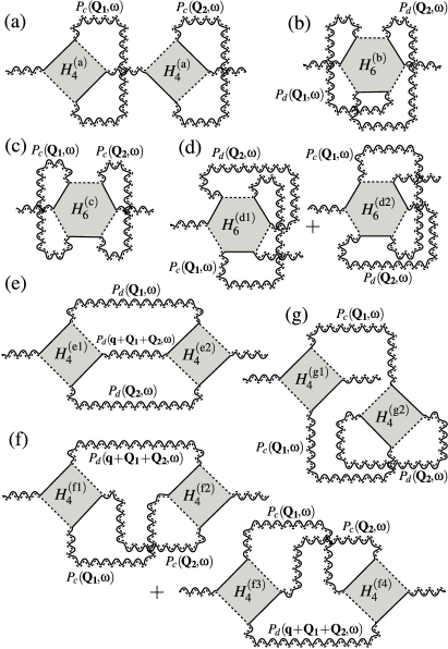
Figure 3: Diagrams contributing to the two-loop correction $\,\chi_{\rm GCE}^{(2)}$. Answers for the Hikami boxes read: $H_{4}^{\rm(a,g1)}={\cal D}{\bf{q}}^{2}$,  $H_{6}^{\rm(b,c)}=-\tau^{2}{\cal D}{\bf{q}}^{2}$,  $H_{6}^{\rm(d1,d2)}=0$,  $H_{4}^{\rm(e1)}\times H_{4}^{\rm(e2)}=({\cal D}({\bf{q}}({\bf{q}}+{\bf{Q_{1}}}+{\bf{Q_{2}}})))^{2}$,  $H_{4}^{\rm(f1)}\times H_{4}^{\rm(f2)}=H_{4}^{\rm(f3)}\times H_{4}^{\rm(f4)}=2{\cal D}^{2}({\bf{q}}{\bf{Q_{1}}})({\bf{q}}{\bf{Q_{2}}})$, and $H_{4}^{\rm(g2)}={\cal D}({\bf{Q_{1}}}^{2}+\gamma/D)$, see the main text for details. Here $\,{\cal D}=4\pi\rho\tau^{4}D$.

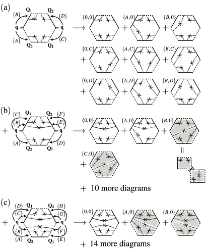
Figure 4: Dressing of the 6-point Hikami box of Fig. 3(b) using the algorithm introduced in Fig. 2. (a) Only 8 of the 15 dressings are generated by moving the vertices. The other dressings are generated by adding one (b) or two (c) impurity lines, followed by repeating the procedure. This algorithm also generates products of 4-point Hikami boxes, indicated by a gray box. Summing up all 40 diagrams yields $-12\pi\rho\tau^{6}D{\bf{q}}^{2}$.

To calculate the subleading quantum corrections, one has to consider the two-loop diagrams shown in Fig. 3, which contain momentum sums over diffuson or Cooperon propagators, or both. Thus, their contribution is subleading in either $(\Delta/\max(\omega,\gamma))$, $(\Delta/\omega)$, or $(\Delta/D{\bf{q}}^{2})$. Note that the diagrams containing only diffusons are not relevant for the experiments, since they are magnetic field independent. We have used the algorithm described above to calculate the 4-point Hikami-boxes $H_{4}^{(a)-(g1)}$ of Fig. 3 avoiding double-counting and maintaining electroneutrality, Eq. (6). The “inner” Hikami box of Fig. 3(g), $H_{4}^{(g2)}$, is of different nature because it is connected to two internal Cooperons. Nevetheless, the same double counting problem appears and can be overcome with the help of dressing this box by moving the vertices with the attached Cooperons. As a result, electroneutrality does not necessarily apply for $H_{4}^{(g2)}$, which is reflected by its $\,\gamma$-dependence, see the next paragraph. Besides, the diagrams shown in Fig. 3(b-d) contain 6-point Hikami boxes. Their dressing is more subtle because of two issues, see the example shown in Fig. 4, which corresponds to the Hikami box $H_{6}^{\rm(b)}$ of Fig. 3(b): First, starting with the undressed diagram and moving vertices into the attached diffusons, one cannot generate all required 15 dressings shown in Fig. 1(c). Instead, only 8 dressings can be obtained for the 6-point Hikami box, cf. Fig. 4(a). That problem can be solved by considering two more “skeleton diagrams” with one-, Fig. 4(b), and two-, Fig. 4(c), additional impurity lines between GFs of the same retardation. All of the missing dressings can be obtained by applying the above described algorithm similar to Fig. 4(a). Second, by moving the vertices of the diagrams in Figs. 4(b,c) new diagrams of the same order in $({\epsilon_{\rm F}}\tau)^{-1}\ll 1$ are generated, which look like products of two dressed or undressed 4-point Hikami boxes with a few-impurity ladder in-between. Several examples are highlighted by grey boxes in Figs. 4(b,c). It is not a priori clear whether such diagrams belong to the diagram shown in Fig. 3(b) or Fig. 3(e). However, keeping them only in the diagram Fig. 3(b) allows us to maintain the electroneutrality in all two-loop diagrams. The total result for $H_{6}^{\rm(b)}$ is obtained by summing 40 generated diagrams. The 6-point Hikami boxes of Figs. 3(c,d) can be calculated analogously.

Before presenting the final answer, we would like to discuss how to reinstate the finite dephasing rate in the equations. First, $\,\gamma\,$ must be included as a mass term in all Cooperon propagators. Second, when calculating the Hikami box $H_{4}^{\rm(g2)}$ of Fig. 3(g), only the number of coherent modes has to be conserved. The latter is in contrast to all other Hikami boxes, which obey the usual electroneutrality condition, i.e., the conservation of the total number of particles. Hence, $H_{4}^{\rm(g2)}$ is the only Hikami box of the two-loop calculations which is sensitive to dephasing of the Cooperons. This statement can be checked directly with the help of the model of magnetic impurities. Introducing a slightly reduced scattering rate for all elastic collisions in the particle-particle channel, $1/\tau\to 1/\tau-\gamma_{\rm mi}$, where $\gamma_{\rm mi}\ll 1/\tau$, and keeping $1/\tau$ for collisions in the particle-hole channel, we observe that the Cooperon acquires the mass $\gamma_{\rm mi}$ since magnetic scattering breaks time-reversal symmetry. Hence, magnetic scattering rate is similar to the dephasing rate; they both provide consistent infrared cut-offs for Cooperons. Applying the algorithm described above, we find that, among all the two-loop diagrams in Fig. 3, the rate $\gamma_{\rm mi}$ appears only in the expressions for Cooperons and in the Hikami box $H_{4}^{(g2)}$. In the latter case, it leads to changing $D{\bf{Q_{1}}}^{2}$ to $D{\bf{Q_{1}}}^{2}+\gamma_{\rm mi}$. Using the analogy between magnetic scattering and dephasing, we conclude that $\gamma$ enters $H_{4}^{(g2)}$ in the same way.

Omitting lengthy and tedious algebra which will be published elsewhere, together with a detailed proof of the validity of our method and an analysis of the IR cut-off in systems with magnetic impurities, the answer for $\,\delta\chi_{\rm GCE}^{(2)}\,$ reads:

$$\delta\chi_{GCE}^{(2)}({\bf{q}},\omega)=\frac{1}{(2\pi)^{2}\rho_{0}V^{2}}\frac{2i\omega D{\bf{q}}^{2}}{(D{\bf{q}}^{2}-i\omega)^{2}}\sum_{{\bf{Q_{1}}},{\bf{Q_{2}}}}\Big{[}$$ (18)

$$P_{c}({\bf{Q_{1}}},\omega)P_{c}({\bf{Q_{2}}},\omega)\ \left(\frac{D{\bf{q}}^{2}+i\omega}{D{\bf{q}}^{2}-i\omega}+\frac{4D({\bf{q}}{\bf{Q_{1}}})({\bf{q}}{\bf{Q_{2}}})/{\bf{q}}^{2}}{D({\bf{q}}+{\bf{Q_{1}}}+{\bf{Q_{2}}})^{2}-i\omega}\right)$$

$$+P_{d}({\bf{Q_{1}}},\omega)P_{d}({\bf{Q_{2}}},\omega)\ \left(\frac{2D[{\bf{q}}({\bf{q}}+{\bf{Q_{1}}}+{\bf{Q_{2}}})]^{2}/{\bf{q}}^{2}}{D({\bf{q}}+{\bf{Q_{1}}}+{\bf{Q_{2}}})^{2}-i\omega}-1\right)$$

$$+P_{c}({\bf{Q_{1}}},\omega)P_{d}({\bf{Q_{2}}},\omega)\ \left(2+2i\omega\,P_{c}({\bf{Q_{1}}},\omega)\right)\ \Big{]}\,.$$

To conclude this section, we would like to note that our method of dressing the Hikami boxes goes far beyond the initial ideas of LABEL:Hastings_Inequivalence_1994. It is a very powerful and generic working tool which can be extended to even more complicated diagrams, including higher loop corrections, and nontrivial physical problems. For example, our method can be straightforwardly used to describe mesoscopic systems in the ballistic regime, cf. LABEL:Zala_Interaction_2001. Therefore, the diagrammatic approach presented above is complimentary to the diffusive nonlinear $\,\sigma$-model which fails to yield ballistic results. One can invent alternative digrammatic tricks which help to avoid the complexity of the Hikami boxes with scalar vertices. For instance, the density response function can be obtained by calculating the current response function (averaged conductivity) first and then using the continuity equation. In the latter approach, the dressed scalar vertices are replaced by undressed vector ones, which greatly simplifies the calculationGorkov_Conductivity_1979 . However, this method cannot describe the full ${\bf{q}}$-dependence of $\,\chi$, which is crucial for the polarizability. We have checked that both approaches give the same results in the small-${\bf{q}}$ limit.

III.2 Canonical ensemble

In this section, we study the disorder average of the density response function $\chi$ in the CE, where the number of particles $N$ is fixed in each sample. Let us first discuss the properties of the statistical ensemble which corresponds to the experimental measurements of the polarizability, such as the experiment discussed in Section VI. We are mainly interested in the behavior close to the 0D regime, where due to $\,\tau_{\varphi}\geq 1/E_{\rm Th}$, there is no self-averaging. Instead, the disorder average is usually realized by an ensemble average. The samples from the ensemble differ in impurity configuration and can have slightly different particle number. At $T=0$ (in the ground state) all single-particle levels below the Fermi level ${\epsilon_{\rm F}}$ are occupied. However, one cannot fix $\,{\epsilon_{\rm F}}\,$ for the whole ensemble due to randomness of the energy levels and due to the fluctuations of $\,N\,$ from sample to sample. This can be taken into account by introducing an ${\epsilon_{\rm F}}$ which fluctuates around the typical value $\,\mu^{0}$;Lehle_Canonical_1995 $\,\mu^{0}$ fixes the mean value of $\,N\,$ in the entire ensemble. It has been shown that such ensembles of isolated disordered samples with fluctuating ${\epsilon_{\rm F}}$ can be described by the so-called Fermi-level pinning ensemble, Lehle_Canonical_1995 ; Altland_Canonical_1992 which is realized as follows: (i) the Fermi-energy is pinned to an energy level $\epsilon_{\bf{k}}$, such that ${\epsilon_{\rm F}}=\epsilon_{\bf{k}}+0$. (ii) the level $\epsilon_{\bf{k}}$ is sampled from a weight function $P(\epsilon_{\bf{k}})$, which is centered at $\mu^{\,0}$ and is normalized: $\,\int P(\epsilon){\rm d}\epsilon=1$. The support of $P(\epsilon_{\bf{k}})$ should be much smaller than $\mu^{\,0}$ but much larger than $\Delta$. The correlations resulting from fixing $\,N\,$ in the given sample are subsequently reduced to the additional correlations induced by disorder with the help of the following procedure: The expression for the density response function averaged over the fluctuating Fermi energies and over disorder reads:

$$\overline{\chi}({\bf{q}},\omega)= \frac{1}{\sum_{\bf{k}}\overline{P(\epsilon_{\bf{k}})}}\sum_{\bf{k}}\overline{P(\epsilon_{\bf{k}})\chi_{\epsilon_{\bf{k}}}({\bf{q}},\omega)}\,.$$ (19)

In Eq. (19) we have assumed that the numerator and denominator can be averaged over disorder independently, see the discussion in LABEL:Lehle_Canonical_1995. Since the averaged density of states depends only weakly on disorderMontambaux_Book_2007 and is almost constant on the support of $\,P$, the denominator of Eq. (19) can be simplified

$$\sum_{\bf{k}}\overline{P(\epsilon_{\bf{k}})}=V\int_{-\infty}^{+\infty}\!{\rm d}E\,P(E)\overline{\rho_{E}}\approx\rho_{0}V\,.$$ (20)

Inserting Eq. (8) and Eq. (20) into Eq. (19), we find the disorder averaged density response function in the CE:

$$\overline{\chi}({\bf{q}},\omega)=\frac{1}{\rho_{0}}\int_{-\infty}^{+\infty}\!{\rm d}E\,P(E)\overline{\rho_{E}\,\chi_{E}({\bf{q}},\omega)}=\overline{\chi}_{\mu}+\delta\chi_{CE}\,.$$ (21)

The loop-expansion of $\,\overline{\chi}_{\mu}\,$ was calculated in the previous section. The quantity $\,\delta\chi_{CE}\,$ describes additional contributions resulting from fluctuations of $\,{\epsilon_{\rm F}}$. It is governed by the irreducible part of the integrand:

$$\delta\chi_{CE} \equiv \frac{1}{\rho_{0}}\int_{-\infty}^{+\infty}\!{\rm d}E\,P(E)\left(\overline{\rho_{E}\,\chi_{E}({\bf{q}},\omega)}-\overline{\rho_{E}}\,\overline{\chi_{E}({\bf{q}},\omega)}\right)$$ (22)

$$\simeq \frac{1}{\rho_{0}}\left(\overline{\rho_{E}\,\chi_{E}({\bf{q}},\omega)}-\rho_{0}\,\overline{\chi_{E}({\bf{q}},\omega)}\right)\,.$$

In Eq. (22), we have assumed that the disorder-averaged quantities are (almost) independent of the absolute values of the particle energies. As a result, the exact form of the weight function $P(\epsilon_{\bf{k}})$ is not important. Let us now derive the leading contribution to $\,\delta\chi_{CE}$.

Figure 5: Diagrammatic representation of the term $\rho_{E}\,\chi_{E}({\bf{q}},\omega)$ from Eq. (22) before impurity averaging, cf. Eqs. (8,9).

Diagrammatically, the additional factor $\,\rho_{E}\,$ in Eq. (22) is represented as a closed fermionic loop with a vertex between two (disorder averaged in further calculations) GFs which have the same retardation, energy and momentum, see Fig. 5. Following LABEL:Smith_Spectral_1998, we greatly reduce the number of possible diagrams in Eq. (22) by generating this vertex with the help of an additional energy derivative:

$$\overline{G}^{R/A}_{\epsilon}({\bf{k}})^{2}=-\lim_{\lambda\to 0}\dfrac{\partial}{\partial\lambda}\overline{G}^{R/A}_{\epsilon+\lambda}({\bf{k}})\,.$$ (23)

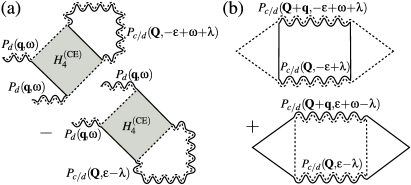
Figure 6: One-loop diagrams which contribute to the disorder averaged $\,\delta\chi_{CE}$, Eq. (22), before taking the derivative $\partial/\partial\lambda$, cf. Eq. (23). Both 4-point Hikami boxes in (a) are given by $H_{4}^{\rm(CE)}=2\pi\rho_{0}\tau^{4}(D{\bf{q}}^{2}-i\omega)$.

After disorder averaging, we find two types of one-loop diagrams which contribute to $\,\delta\chi_{CE}$, see Fig. 6: (i) the diagrams in Fig. 6(a) are obtained by pairing the closed loop with the $G^{R}G^{A}$ terms of $\chi_{E}$ (first term of the second line of Fig. 5); (ii) the diagrams of Fig. 6(b) result form pairing with the $G^{R}G^{R}$/$G^{A}G^{A}$ terms (second and third term). Furthermore, 4 more diagrams can be constructed where Cooperon propagators are replaced by diffuson ones.

The double-counting problem does not appear in the diagrams in Fig. 6(a), which contain 4-point Hikami boxes. Therefore, the method which we used for the GCE diagrams is not needed here. The only subtle issue in their calculation is that the diagrams are small if the closed loop, $\,\rho_{E}$, is connected to the bubble, $\,\chi_{E}$, by only one single impurity line. Thus, at least two such connections must be taken into account either in the ladder (which starts then from two impurities) or in the ladder (which can start from one impurity) and the particular dressing of the Hikami box which connects $\rho_{E}$ to $\chi_{E}$. Furthermore, the 4-point Hikami box in Fig. 6(a) does not acquire a dependence on dephasing rate $\gamma$, which can be checked with the help of the model of magnetic impurities discussed before Eq. (18). As a result, $\gamma$ has to be included only as a mass term in the connected Cooperon.

Summing up all parts and calculating the auxiliary derivative, Eq. (23), we obtain the one-loop answer for $\,\delta\chi_{CE}$:

$$\delta\chi_{CE}^{(1)}({\bf{q}},\omega)=\frac{2}{(2\pi)^{2}\rho_{0}V^{2}}\sum_{\alpha=c,d}\sum_{\bf{Q}}$$ (24)

$$\quad\times\Big{[}\tfrac{i\omega}{D{\bf{q}}^{2}-i\omega}P_{\alpha}({\bf{Q}},\omega)P_{\alpha}({\bf{Q}},0)+P_{\alpha}({\bf{Q}}+{\bf{q}},\omega)P_{\alpha}({\bf{Q}},0)\Big{]}\,.$$

Electroneutrality is restored in Eq. (24) after summing all the diagrams of Fig. 6. Thus, all contributions, Eqs. (17), (18) and (24), obey the electroneutrality condition; therefore, $\,\overline{\chi}({\bf{q}}=0,\omega)=0$.

Note that the one-loop contribution $\,\delta\chi_{CE}^{(1)}$, (24) is of the same order in $(\Delta/\max(\omega,\gamma))$, $(\Delta/\omega)$ or $(\Delta/D{\bf{q}}^{2})$ as the two-loop contribution $\,\delta\chi_{GCE}^{(2)}$, Eq. (18). As a result, the differences between GCE and CE disappear at large frequencies $\omega\gg\Delta$, in agreement with LABEL:Noat_Polarizability_1996. At smaller frequencies and weak dephasing, $\max(\omega,\gamma)\lesssim\Delta$, $\,\delta\chi_{GCE}^{(2)}$ is needed to analyze the difference between the GCE and the CE for energies of the order of $\,O(\Delta)$. In the following, we will often refer to $\delta\chi_{GCE}^{(1)}$ as the result from “1st order” perturbation theory, and $\delta\chi_{GCE}^{(1)}+\delta\chi_{GCE}^{(2)}+\delta\chi_{CE}^{(1)}$ (or $\delta\chi_{GCE}^{(1)}+\delta\chi_{GCE}^{(2)}$) as the result from “2nd order’ perturbation theory for isolated (or connected) systems.

IV Quantum corrections to the polarizability

The quantum corrections to $\,\alpha\,$ can be found after inserting the decomposition $\,\chi=\chi_{0}+\delta\chi\,$ into Eq. (5) and expanding the density response function in the RPA, $\,\chi/\epsilon$, in $\,\delta\chi$. Note that the latter can contain $\,\delta\chi_{GCE}^{(1,2)}\,$ and $\,\delta\chi_{CE}^{(1)}\,$ depending on the ensemble which we consider and on the accuracy of the loop-expansion. This expansion up to terms of order $\,O(\delta\chi)^{2}\,$ yields:

$$\frac{\chi({\bf{q}},\omega)}{\epsilon({\bf{q}},\omega)}\approx\frac{\chi_{0}({\bf{q}},\omega)}{\epsilon_{0}({\bf{q}},\omega)}\Bigg{[}1 +\frac{1}{\epsilon_{0}({\bf{q}},\omega)}\frac{\delta\chi({\bf{q}},\omega)}{\chi_{0}({\bf{q}},\omega)}$$ (25)

$$+\frac{1-\epsilon_{0}({\bf{q}},\omega)}{\epsilon_{0}({\bf{q}},\omega)^{2}}\left(\frac{\delta\chi({\bf{q}},\omega)}{\chi_{0}({\bf{q}},\omega)}\right)^{2}\Bigg{]}\,,$$

where $\epsilon_{0}({\bf{q}},\omega)=1-2U({\bf{q}})\chi_{0}({\bf{q}},\omega)$. To separate the frequency dependence due to classical diffusive screening from the frequency dependence of the quantum corrections, it is convenient to rewrite Eq. (25) as follows:

$$\frac{\chi({\bf{q}},\omega)}{\epsilon({\bf{q}},\omega)}\approx\ \rho_{0}S({\bf{q}},\omega)\bigg{[} 1+2\frac{S({\bf{q}},\omega)}{g(|{\bf{q}}|^{-1})}F({\bf{q}},\omega)$$ (26)

$$+8\,U({\bf{q}})\chi_{0}({\bf{q}},\omega)\frac{S({\bf{q}},\omega)^{2}}{g(|{\bf{q}}|^{-1})^{2}}F({\bf{q}},\omega)^{2}\bigg{]}\,.$$

Here we have introduced two dimensionless functions:

$$S({\bf{q}},\omega)\equiv\left(\!\!1\!-\!2U({\bf{q}})\rho_{0}\!-\!\frac{i\omega}{D{\bf{q}}^{2}}\!\!\right)^{\!\!\!-1}\,,$$ (27)

which describes classical diffusive screening, and

$$F({\bf{q}},\omega)\equiv \frac{(D{\bf{q}}^{2}-i\omega)^{2}}{D{\bf{q}}^{2}}\pi V\,\delta\chi({\bf{q}},\omega)\,,$$ (28)

which describes the quantum corrections to $\,\chi$. $\,g(L)\,$ denotes the dimensionless conductance of a diffusive system of size $L$:

$$g(L)\equiv 2\pi\,E_{\rm Th}\!(L)/\Delta\,,\quad E_{\rm Th}\!(L)=D/L^{2}\,.$$ (29)

Eqs. (26)-(28) together with Eqs. (17), (18) and (24) are the first major results of this paper. The quantum corrections $\Delta\alpha$ are obtained by substituting the terms $\sim F$ and $\sim F^{2}$ of Eq. (26) into Eq. (5) and summing over ${\bf{q}}$. We remind the reader that the zero mode does not contribute to the polarizability due to electroneutrality $\,\chi({\bf{0}},\omega)=0$ and, therefore, we can assume $\,|{\bf{q}}|\neq 0\,$ in Eq. (26). The typical momenta which govern the sum in Eq. (5) are $\,|{\bf{q}}|\sim 1/L\,$ since the external potential $\phi_{\rm ext}$ varies on the scale of the sample size $L$. But we will keep $\,{\bf{q}}\,$ below for generality.

V Comparison to RMT+$\sigma$-model

Let us now compare the results of our perturbative calculations with those of LABEL:Blanter_Polarizability_1998 which are obtained from a combination of the RMT approach and the nonlinear $\sigma$-model. The latter will be referred to as “RMT+$\sigma$-model”. This comparison requires an assumption $\,E_{\rm Th}(L)\gg\max(\Delta,\omega,\gamma)\,$ which in particular means $\,g(L)\to\infty$. In this limit, the term $\,\sim F^{2}\,$ in Eq. (26) acquires an additional smallness (which can be estimated as $\,O(1/g(L))$) and can be neglected while the term $\,\sim F^{1}\,$ becomes independent of ${\bf{q}}$. Next, we keep only the zero mode contributions in all sums over internal momenta in the expressions for $\,\chi_{GCE}^{(1,2)}\,$ and $\,\delta\chi_{CE}^{(1)}\,$ and consider the difference of $\,F\,$ calculated for unitary and orthogonal ensembles: $\,\delta_{B}F(\omega)=F(\omega,B\to\infty)-F(\omega,0)$, where $B$ is the strength of an external magnetic field. The terms which contain only diffusons are canceled in $\,\delta_{B}F$.

Using Eqs. (17), (18) and (24), we obtain

$$\delta_{B}F(\omega, g\to\infty)=$$ (30)

$$\underbrace{-\frac{i\omega}{\gamma-i\omega}}_{\delta\chi_{GCE}^{(1)}}-\frac{\Delta}{2\pi}\Big{[}\underbrace{\frac{i\omega-2\gamma}{(\gamma-i\omega)^{2}}}_{\delta\chi_{GCE}^{(2)}}+\underbrace{\frac{2\gamma}{\gamma(\gamma-i\omega)}}_{\delta\chi_{CE}^{(1)}}\Big{]}\,.$$

Subscripts under the braces explain the origin of the corresponding terms. The last term must be taken into account only in the CE. The counterpart of Eq. (30) obtained from RMT+$\sigma$-model in LABEL:Blanter_Polarizability_1998 reads:

$${\rm RMT+\sigma:}\quad\delta_{B}F(\omega)=1+\int_{+0}^{\infty}\frac{\!{\rm d}\epsilon\,}{\Delta}\left(\frac{1}{\epsilon-\omega}+\frac{1}{\epsilon+\omega}\right)$$ (31)

$$\times\left[\overbrace{\underbrace{\epsilon\,\delta_{B}R_{2}(\epsilon)}_{GCE}+\Delta\,\delta_{B}R_{2}(\epsilon)+\int_{+0}^{\epsilon-0}\!{\rm d}\epsilon_{1}\,\,\delta_{B}\tilde{R}_{3}(\epsilon,\epsilon_{1})}^{CE}\right]\,.$$

Here $R_{2,3}$ are the usual (dimensionless) two- and three-level spectral correlation functions, $\tilde{R}_{3}(\epsilon,\epsilon_{1})=R_{3}(\epsilon,\epsilon_{1})-R_{2}(\epsilon)\,$, and $\,\delta_{B}R_{2,3}$ denotes the difference of the correlation functions without and with time-reversal symmetry. We have marked in Eq. (31) the relevance of different terms for the GCE and the CE.

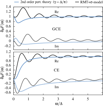
Figure 7: (color online) The quantum corrections to the polarizability in the limit $\,E_{\rm Th}\!(L)\gg\max(\Delta,\omega,\gamma)\,$ for the GCE (upper panel) and the CE (lower panel). We compare real (solid lines) and imaginary (dashed lines) parts the function $\delta_{B}F$ obtained from 2nd order perturbation theory, Eq. (30), and from the RMT+$\sigma$-model, Eq. (31).

We remind the reader that the RMT+$\sigma$-model results are valid for $\,\gamma=0\,$ and cannot straightforwardly describe a $\gamma$-dependence, while our perturbative result, Eq. (30), is valid only if $\Delta\lesssim{\rm max}\left(\gamma,\omega\right)$. To resolve this issue, one should set in Eq. (30) $\gamma\sim\Delta$. Eq. (30) yields $\,\delta_{B}F(\omega\to 0,g\to\infty)=\Delta/(\pi\gamma)$ for the GCE. Therefore, we have chosen $\,\gamma=\Delta/\pi\,$ to ensure the correct limit $\,\delta_{B}F(\omega\to 0,g\to\infty)\big{|}_{GCE}=1$.

The comparison of the results obtained from RMT+$\sigma$-model and from the perturbative calculations are shown in Fig. 7 for the GCE and the CE. Apart from the oscillations in the RMT+$\sigma$-curves, whose origin is nonperturbative, the agreement is excellent. The asymptotic limits are fully recovered in the perturbative calculations: (i) $\delta_{B}F(\omega\gg\Delta,g\to\infty)\to 1\,$ for the both ensembles; (ii) $\delta_{B}F(\omega~{}\to~{}0,g\to\infty)\to 0\,$ in the CE due to cancellation of $\,\delta\chi^{(2)}_{GCE}\,$ and $\,\delta\chi^{(1)}_{CE}$. The latter property of the CE holds true at any $\gamma$ in 1st and 2nd order perturbation theory. In the GCE, on the other hand, the quantum corrections remain finite for $\omega\to 0$ in 2nd order perturbation theory, in full agreement with the nonperturbative results of LABEL:Blanter_Polarizability_1998 Noat_Comment .

We conclude this section by noting that the perturbation theory is able to reproduce the results of the RMT+$\sigma$-model with good qualitative agreement, which is the second major result of our work.

VI Polarizability of an ensemble of rings

The experiments described in Ref. [Deblock_Experiment_2000, ] and [Deblock_Experiment_2002, ] were done on a large number of disordered metallic rings. The rings were etched on a 2D substrate and were placed on the capacitative part of a superconducting resonator, where a spatially homogeneous in-plane electric field ${\bf{E}}(\omega)$ acted on them. In terms of the coordinate along the ring, $x\in[0,2\pi R]$, where $R$ is the ring radius, the external electric potential of this field is $\phi_{\rm ext}(x,\omega)=|{\bf{E}}(\omega)|R\cos(x/R)+\phi_{\rm ext}^{(0)}$, and its Fourier transform reads

$$\phi_{\rm ext}(q,\omega)=-|{\bf{E}}(\omega)|R^{2}\pi\left[\delta_{q,1/R}+\delta_{q,-1/R}\right]+\phi_{\rm ext}^{(0)}\cdot\delta_{q,0}\,.$$ (32)

The constant shift of the potential $\,\phi_{\rm ext}^{(0)}\,$ does not contribute to the polarizability. Therefore, the sum in Eq. (5) involves only two modes, $q=1/R$ and $q=-1/R$, which yield

$$\alpha(\omega) = \frac{4e^{2}}{|{\bf{E}}(\omega)|^{2}}\frac{1}{2\pi R}\phi^{2}_{\rm ext}(q,\omega)\frac{\chi(q,\omega)}{\epsilon(q,\omega)}\Big{|}_{q=1/R}$$ (33)

$$= 2\pi e^{2}R^{3}\frac{\chi(1/R,\omega)}{\epsilon(1/R,\omega)}\,.$$

In Eq. (33), we have taken into account the symmetry of the summand under the inversion $\,q\to-q$.

The Coulomb potential in quasi-1D is given by

$$U(q)=2e^{2}\ln(|qW|)\,,\quad|qW|\ll 1\,;$$ (34)

where $\,W\ll R\,$ is the width of the ring. Inserting Eq. (34) into Eq. (27), we find the screening function of the quasi-1D ring at $\,q=1/R$:

$$S(1/R,\omega) =\left(1+(\kappa W)\ln(R/W)/\pi-\frac{i\omega}{E_{\rm Th}\!(R)}\right)^{-1}$$ (35)

$$\overset{\kappa W\gg 1}{\approx}\frac{\pi}{(\kappa W)\ln(R/W)}\equiv S_{0}\ll 1\,.$$ (36)

We have introduced the 2D Thomas-Fermi screening vector, $\kappa=4\pi e^{2}\rho_{0}/W\,$ with $\,\rho_{0}\,$ being the quasi-1D density of states, see e.g. LABEL:Montambaux_Book_2007, and assumed sufficiently strong screening, $\kappa W\gg 1$, such that $\,S\,$ reduces to the $\,\omega$-independent constant $\,S_{0}$. This agrees with the experiment where one can estimate $(\kappa W)\ln(R/W)\approx 18$. Therefore, we focus below only on the limit of strong screening. Note that in this limit, the product $\,U(1/R,\omega)S(1/R,\omega)\,$ can be also simplified

$$U(1/R,\omega)\,S(1/R,\omega)\approx-1/2\rho_{0}\,.$$ (37)

The classical part of the polarizability comes from inserting the leading term of the expansion (26) into Eq. (33):

$$\alpha_{0}\simeq 2\pi e^{2}R^{3}\,\rho_{0}S_{0}=\frac{\pi R^{3}}{2\ln(R/W)}\,.$$ (38)

Using Eqs. (13,37) in Eq. (26), and inserting the result into Eq. (33), we obtain the quantum corrections to the polarizability up to the term $\,\sim(F/g)^{2}$:

$$\frac{\Delta\alpha(\omega)}{2S_{0}\alpha_{0}}\approx\frac{F(R^{-1},\omega)}{g(R)}-2\frac{E_{\rm Th}\!(R)}{E_{\rm Th}\!(R)-i\omega}\left(\frac{F(R^{-1},\omega)}{g(R)}\right)^{\!\!2}.$$ (39)

Let us regroup the terms in Eq. (39) to single out the terms of 1st and 2nd order perturbation theory:

$$\frac{\Delta\alpha(\omega)}{2S_{0}\alpha_{0}}\approx \frac{1}{g(R)}\left(F^{(1)}(1/R,\omega)+F^{(2)}(1/R,\omega)\right)$$ (40)

with

$$F^{(1)}(1/R,\omega)=(2\pi^{2}R)\frac{(E_{\rm Th}\!(R)-i\omega)^{2}}{E_{\rm Th}\!(R)}\delta\chi_{GCE}^{(1)}(1/R,\omega),$$ (41)

and

$$F^{(2)}(1/R,\omega)=$$ (42)

$$\ \ (2\pi^{2}R)\frac{(E_{\rm Th}\!(R)-i\omega)^{2}}{E_{\rm Th}\!(R)}\left(\delta\chi_{GCE}^{(2)}(1/R,\omega)+\delta\chi_{CE}^{(1)}(1/R,\omega)\right)$$

$$\ \ +\frac{2}{g(R)}(2\pi^{2}R)^{2}\frac{(E_{\rm Th}\!(R)-i\omega)^{3}}{E_{\rm Th}\!(R)}\left(\delta\chi_{GCE}^{(1)}(1/R,\omega)\right)^{2}\,.$$

We emphasize that all three parts of the density response function, $\,\delta\chi_{GCE}^{(1,2)}\mbox{ and }\delta\chi_{CE}^{(1)}$, are generically important for the theoretical description of the experimental data with the help of Eq. (40) if the rings are isolated. Having obtained Eqs. (17), (18) and (24) (and Eq. (30) for the limit $g\to\infty$) and Eqs. (39)-(42), we are now in the position to analyze different options to fit the experimental data. Ref. [Deblock_Experiment_2000, ] and [Deblock_Experiment_2002, ] focused on the $T$-dependence of the real part of the quantum corrections, thus, in the following we will concentrate on ${\rm Re}\Delta\alpha$.

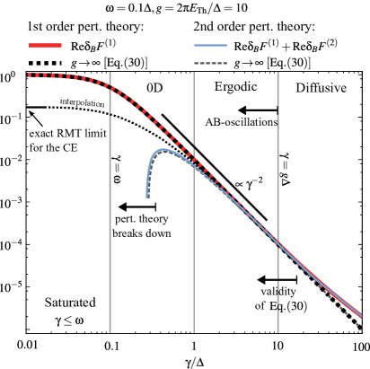
Figure 8: (color online) Comparison of perturbative 1st order, $\delta_{B}F^{(1)}$, 2nd order, $\delta_{B}F^{(1)}+\delta_{B}F^{(2)}$, and interpolated (to the RMT+$\sigma$-model limit) results for the quantum corrections to the polarizability in the parameter range $\omega<\Delta<E_{\rm Th}$.

Figure 9: (color online) Comparison of perturbative 1st order, $\delta_{B}F^{(1)}$, 2nd order, $\delta_{B}F^{(1)}+\delta_{B}F^{(2)}$, and interpolated (to the RMT+$\sigma$-model limit) results for the quantum corrections to the polarizability (a) as a function of $\gamma$ for different values of $\omega$ and (b) as a function of $\omega$ for different values of $\gamma$.

The crossover to 0D dephasing occurs when $\gamma$ decreases below $\Delta$. We expect that the ideal parameter range to study this crossover experimentally in the CE is $\,\omega<\Delta<E_{\rm Th}$. However, it is important that the conductance should be only moderately large, since $\Delta\alpha$ is suppressed in the case of extremely large $\,g$, cf. Eq. (39); and the frequency should not be too small, since the quantum corrections to the polarizability of isolated systems are suppressed in the static limit, see Fig. 7. Let us first discuss our general expectations for this parameter range, which are illustrated in Fig. 8. The simplest regime is $\,1\lesssim\gamma/\Delta\lesssim g\,$ where the loop-expansion can be justified and the difference between the GCE and the CE is negligible. Keeping only the leading term, we obtain a power law for the dependence of $\,\Delta\alpha\,$ on $\,\gamma$. This power law can be derived straightforwardly after noting that, in the range $(\gamma,\omega)/\Delta\ll g$, one can use the approximation Eq. (30) and find ${\rm Re}\Delta\alpha\sim{\rm Re}\delta_{B}F(\omega)\sim\omega^{2}/\gamma^{2}$ for $\omega\ll\gamma$.

The subleading terms, which in particular describe the difference of the GCE and the CE, are able to improve the theoretical answer for $\,\gamma\,$ being slightly smaller than $\,\Delta$. However, $\,{\rm Re}\delta_{B}F^{(2)}\,$ (and, correspondingly, the difference between the ensembles) is small at any $\,\gamma\,$ for moderately small frequencies, see the example $\,\omega=0.4\Delta\,$ in Fig. 9. Therefore, $\,\delta_{B}F^{(1)}\,$ suffices to fit the experiment at $\omega\gtrsim 0.4\Delta$. The $\,T$-dependence of $\,\Delta\alpha\,$ saturates to the value predicted by the RMT$+\sigma$-model at $\,\gamma\lesssim\omega$ which makes the range of pronounced 0D dephasing ($\omega\lesssim\gamma\lesssim\Delta$) too narrow even at $\,\omega\simeq 0.4\Delta$, thus, smaller frequencies are needed. Of course, the perturbation theory is no longer valid if both $\,\omega\,$ and $\,\gamma\,$ are small. In particular, when $\,F^{(2)}\,$ becomes of order of $\,F^{(1)}\,$ it can lead to changing the overall sign of $\,{\rm Re}\delta_{B}(F^{(1)}+F^{(2)})$, see the cut of the lines in Fig. 8 marked “pert. theory breaks down”. We believe that this sign change is unphysical and, moreover, it contradicts the prediction of the RMT+$\sigma$-model. Nevertheless, our calculations show that the power law, which is obtained in the perturbative region from the leading correction, can be extended well into the nonperturbative region $\omega\lesssim\gamma\lesssim\Delta$. This provides us with the unique possibility to detect the crossover to 0D dephasing directly from the amplitude of $\Delta\alpha$. It is in sharp contrast to the quantum corrections to the conductivity, which always saturate at $\gamma\lesssim\Delta$. Treiber_DimensionalCrossover_2009 ; Treiber_QuantumDot_2012

Let us illustrate our unexpected statement with the help of Fig. 8: We know the exact value of $\,\Delta\alpha\,$ in the limit $\gamma\to 0$ from the RMT+$\sigma$-model and the correct behavior of $\,\Delta\alpha$ for $\,\gamma\,$ being of order of (and slightly below) $\,\Delta$. Using these reference points, one can interpolate the dependence $\,\delta\alpha(\gamma)\,$ for the whole region $\,0<\gamma\lesssim\Delta$. Since the slope of the interpolated curve is only slightly different from the perturbative one for $\,\,\gamma\geq 0.3\Delta$, the leading answer of perturbation theory can be used to detect the crossover to 0D dephasing. If the range $\,\gamma\geq 0.3\Delta$ is not sufficient for unambiguously fitting the experiment, the whole interpolated curve can be used instead.

The authors of Ref. [Deblock_Experiment_2000, ] and [Deblock_Experiment_2002, ] used a superconducting resonator with fixed frequency $\,\omega\simeq 0.2\Delta\simeq 17{\rm mK}\,$ to measure $\,\Delta\alpha(T)\,$ of the rings. In the following we will apply our theory to explain the experimental results of these papers. We note that the qualitative difference in the slope of the curves obtained from the three options for fitting – (i) the interpolated curve, (ii) the result of 2nd order perturbation theory, and (iii) the leading perturbative result – becomes rather insignificant at $\,\omega\simeq 0.2\Delta$ and $\gamma\gtrsim 0.3\Delta$, see Fig. 9(a). The main difference between (i) and (iii) is that the saturation originates at slightly larger $\,\gamma\,$ than the leading perturbative result would suggest. Thus we can safely keep $\,F^{(1)}\,$ and neglect $\,F^{(2)}\,$ to fit the data, which makes our task simpler phi_0_oscillations .

The experimental results for the ring polarizability can be distorted because of a parasitic contribution from the resonator. The latter has been filtered out in the experiment with the help of an additional weak magnetic field $\,B\,$ applied perpendicular to the rings, such that $\Delta\alpha$ becomes a periodic function of the magnetic flux through the ring. Measuring the $T$-dependence of the $\phi_{0}/2$ oscillations, cf. Fig. 9 of LABEL:Deblock_Experiment_2002, allows one to focus purely on the response of the rings. Using Eq. (17) in Eq. (28), we find

$$\Delta\alpha \propto F^{(1)}(1/R,\omega)=i\omega\sum_{\bf{Q}}P_{c}({\bf{Q}},\omega)$$ (43)

$$=i\omega L\int_{0}^{\infty}\!{\rm d}t\,e^{i\omega t}\sum_{n}\frac{1}{\sqrt{4\pi Dt}}e^{-(nL)^{2}/4Dt}e^{i\theta n}e^{-\gamma\,t}\,,$$

where $\theta=4\pi\phi/\phi_{0}$ and $\phi$ is the flux through one ring, and $\,L=2\pi R$. Taking the Fourier transform and selecting the $\phi_{0}/2$ signal gives:

$$\delta_{\phi_{0}/2}F^{(1)}(1/R,\omega)= \frac{i\omega\ {\rm exp}\left(-\sqrt{(\gamma-i\omega)/E_{\rm Th}\!(L)}\right)}{\sqrt{E_{\rm Th}\!(L)(\gamma-i\omega)}}\,.$$ (44)

The function $\delta_{\phi_{0}/2}F^{(1)}$ is shown in Fig. 10(a).

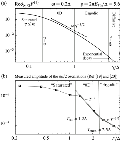
Figure 10: Amplitude of the $\phi_{0}/2$ oscillations. (a) Expected dependence on $\gamma$ from our theory, Eq. (44), for the parameter range $\omega\ll\Delta\ll E_{\rm Th}$. (b) Experimentally measured data as a function of temperature and possible interpretation. Note that the theory (see e.g. Ref. [Treiber_DimensionalCrossover_2009, ] and [Treiber_ThermalNoise_2011, ]) predicts $\gamma_{\rm 0D}\propto T^{2}$ in the 0D regime, and $\gamma_{\rm erg}\propto T$ in the ergodic regime, therefore, the $\gamma^{-3/2}$ behavior indicated in (a) encompasses both the $T^{-3}$ and $T^{-3/2}$ behavior seen in (b).

It is similar to $\delta_{B}F^{(1)}$, cf. Fig. 8, however, the dependence of $\delta_{\phi_{0}/2}F^{(1)}$ on $\gamma$ is governed by a $\propto\gamma^{-3/2}$ power law in the regime $\omega\ll\gamma\ll g\Delta$, and in the regime $g\Delta\ll\gamma$, the $\phi_{0}/2$ oscillations are exponentially suppressed. The theory predicts a 0D dephasing rate, $\gamma_{\rm 0D}=a\Delta T^{2}/E_{\rm Th}^{2}$,Sivan_QuasiParticleLifetime_1994 at low temperatures and an ergodic dephasing rate, $\gamma_{\rm erg}=b\Delta T/E_{\rm Th}$,Ludwig_AharonovBohm_2004 ; Texier_DiffusiveRing_2005 at higher temperatures, where $a$ and $b$ are system-specific, dimensionless coefficients of order $\sim 1$, see Ref. [Treiber_DimensionalCrossover_2009, ] and [Treiber_ThermalNoise_2011, ]. The crossover between the two regimes occurs at a temperature $T_{\rm cross}=\tfrac{b}{a}E_{\rm Th}$. We expect that the saturation at $\gamma=\omega$ occurs in the 0D regime, corresponding to a temperature $T_{sat}=\tfrac{1}{\sqrt{a}}E_{\rm Th}\sqrt{\omega/\Delta}$. Note that the conductance of each ring was rather small, $\,g(L)\approx 5.6\,$, such that the Thouless energy $E_{\rm Th}\!(L)\approx 0.9\Delta$. Thus, depending on the coefficients $a$ and $b$, $T_{\rm cross}$ and $T_{\rm sat}$ can be relatively close to each other.

The experimental result for the $T$ dependence of the $\phi_{0}/2$ oscillations is shown in Fig. 10(b). The measurements were done in the temperature interval $\omega\simeq 0.2\Delta\leq T\leq 4\Delta$. Based on the preceding discussion, we offer the following interpretation of the data: At low temperatures $T\lesssim 1.2\Delta$, the quantum corrections depend only weakly on $T$ and are almost saturated. At intermediate temperatures $1.2\Delta\lesssim T\lesssim 2.5\Delta$ the slope of the data is steep and consistent with 0D dephasing $\Delta\alpha(T)\propto\gamma_{\rm 0D}^{-3/2}\propto T^{-3}$. At higher temperatures $T\gtrsim 2.5\Delta$, the slope of $\Delta\alpha(T)$ decreases and is consistent with ergodic dephasing $\Delta\alpha\propto\gamma_{\rm erg}^{-3/2}\propto T^{-3/2}$. The crossover temperatures, $T_{\rm sat}\simeq 1.2\Delta$ and $T_{\rm cross}\simeq 2.5\Delta$, correspond to coefficients $a\simeq 0.1$ and $b\simeq 0.3$, which are close to the values predicted in LABEL:Treiber_DimensionalCrossover_2009 ($a\simeq 0.04$ and $b\simeq 1$). However, we stress that this interpretation is based only on very few data points, and we do not claim that the experiment clearly shows a crossover to 0D dephasing. Further experiments are needed to support this statement, see Section VII.

VII Conclusions

Understanding interference phenomena and dephasing in mesoscopic systems at very low temperatures is a subtle issue which has provoked controversies between different theoretical approaches Marquardt_Decoherence_2007 , as well as between theory and experiments Huibers_Dephasing_1998 . Quantum transport experiments cannot give a certain answer to all questions because of unavoidable distortions due to the coupling to the environment. The response of isolated disordered samples, on the other hand, provides a “cleaner” setup to study dephasing, and gives one the possibility to settle long-lasting open questions.

We have studied the quantum corrections to the polarizability of isolated disordered metallic samples aiming to improve the explanation of previous experiments (Ref. [Deblock_Experiment_2000, ] and [Deblock_Experiment_2002, ]), and to suggest new measurements, where the elusive 0D regime of dephasing can be ultimately detected. Using the standard strategy of mesoscopic perturbation theory, i.e. the loop-expansion in diffusons and Cooperons, we have developed a theory, which (i) accounts for the difference between connected (GCE) and isolated (CE) systems, and (ii) is able to describe the low frequency response of disordered metals, taking into consideration weak dephasing induced by electron interactions. We have shown that the difference between the GCE and the CE appears only in the subleading terms, therefore, we have extended the calculations up to the second loop. An important by-product of these calculations is a systematic procedure to evaluate the Hikami boxes, see Fig. 2 and 4, which is based on a fundamental conservation lawHastings_Inequivalence_1994 : electroneutrality of the density response function. Our main analytical results for the quantum corrections to the polarizability are presented in Eqs. (26)-(28) with Eqs. (17), (18) and (24).

We have demonstrated that, in the experimentally relevant parameter range, the difference between the statistical ensembles is unimportant and one can fit the measurements by using the leading term of the perturbation theory. The authors of Ref. [Deblock_Experiment_2000, ] and [Deblock_Experiment_2002, ] have tried to find 0D dephasing with the help of an empirical fitting formula. By using the more rigorous and reliable Eq. (44), we have confirmed that 0D dephasing might have manifested itself in the $T$-dependence of magneto-oscillations at $T\lesssim E_{\rm Th}$. Unfortunately, the $T$-range of interest here is rather narrow, and only few experimental data points are available there. Therefore, we are unable to claim conclusively that 0D dephasing has been observed in the experiments. However, we can straightforwardly suggest several experiments which might yield conclusive evidence of 0D dephasing: First, one can repeat the measurement of Ref. [Deblock_Experiment_2000, ] and [Deblock_Experiment_2002, ], but with a larger number of data points around the crossover temperature $T_{\rm cross}$, see Fig. 10, while simultaneously improving the measurements precision. Since the theory predicts a drastic increase in slope of the $\phi_{0}/2$-oscillations at the crossover (from $T^{-3/2}$ to $T^{-3}$), even such measurements should be able to reliably confirm the existence of 0D dephasing, thereby uncovering the role of the Pauli blocking at low $T$. Second, it is highly desirable to extend the $T$-range where the crossover to 0D dephasing is expected to appear, which can be achieved by decreasing $\omega$ and/or increasing $g$. However, a very large conductance and ultra-small frequencies are nevertheless undesirable, because in these limits the quantum corrections to the polarizability are reduced. Thus, improving the precision of the measurement is needed anyway. Besides, fitting with the help of the leading perturbative result fails at very small frequencies, see Fig. 9. This difficulty can be overcome by taking into account our two-loop results and/or using an interpolation to the $\gamma\to 0$ limit from the RMT+$\sigma$-model, see Fig. 8.

To summarize, we have shown that the quantum corrections to the polarizability are an ideal candidate to study dephasing at low $T$ and the crossover to 0D dephasing. We very much hope that our theoretical results will stimulate new measurements in this direction.

- (1) B. L. Altshuler, and A. G. Aronov, in Electron-Electron Interactions in Disordered Systems, edited by A. L. Efros and M. Pollak (North-Holland, Amsterdam, 1985), Vol. 1.
- (2) B. L. Altshuler, A. G. Aronov, and D. E. Khmelnitsky, J. Phys. C 15, 7367 (1982).
- (3) U. Sivan, Y. Imry, and A. G. Aronov, Europhys. Lett. 28, 115 (1994).
- (4) M. Treiber, O. M. Yevtushenko, and J. von Delft, Ann. Physik 524, 188 (2012).
- (5) B. L. Altshuler, Y. Gefen, A. Kamenev, and L. S. Levitov, Phys. Rev. Lett. 78, 2803 (1997).
- (6) Ya. M. Blanter, Phys. Rev. B54, 12807 (1996).
- (7) V. E. Kravtsov, and A. D. Mirlin, JETP Lett. 60, 656 (1994).
- (8) Ya. M. Blanter, and A. D. Mirlin, Phys. Rev. B 57, 4566 (1998); Ya. M. Blanter, and A. D. Mirlin, ibid. 63, 113315 (2001).
- (9) G. Montambaux, and E. Akkermans, Mesoscopic Physics of Electrons and Photons, Cambridge University Press (2007).
- (10) A. Kamenev and Y. Gefen, Phys. Rev. Lett. 70, 1976 (1993); Phys. Rev. B 56, 1025 (1997); A. Kamenev, B. Reulet, H. Bouchiat, and Y. Gefen, Europhys. Lett. 28, 391 (1994).
- (11) W. Lehle, and A. Schmid, Ann. Physik 507, 451 (1995).
- (12) A. Altland, S. Iida, A. Müller-Groeling, and H. A. Weidenmüller, Europhys. Lett. 20, 155 (1992); Ann. Phys. (N.Y.) 219, 148 (1992).
- (13) This approach has also been used in LABEL:Blanter_Polarizability_1998 to describe the polarizability in the nonperturbative regime.
- (14) L. P. Gorkov, and G. M. Eliashberg, Sov. Phys. JETP 21, 940 (1965).
- (15) M. J. Rice, W. R. Schneider, and S. Strässler, Phys. Rev. B 8, 474 (1973).
- (16) A detailed discussion of the assumptions of LABEL:Gorkov_Eliashberg_1965 can be found in: Ya. M. Blanter, and A. D. Mirlin, Phys. Rev. B 53, 12601 (1996).
- (17) K. B. Efetov, Phys. Rev. Lett. 76, 1908 (1996).
- (18) Y. Noat, B. Reulet, and H. Bouchiat, Europhys. Lett. 36, 701 (1996); Y. Noat, R. Deblock, B. Reulet, and H. Bouchiat, Phys. Rev. B 65, 075305 (2002).
- (19) R. Deblock, Y. Noat, H. Bouchiat, B. Reulet, and D. Mailly, Phys. Rev. Lett. 84, 5379 (2000).
- (20) R. Deblock, Y. Noat, B. Reulet, H. Bouchiat, and D. Mailly, Phys. Rev. B 65, 075301 (2002).
- (21) H. Bruus and K. Flensberg, Many-Body Quantum Theory in Condensed Matter Physics, Oxford Graduate Texts in Mathematics (Oxford University Press, 2004).
- (22) D. Vollhardt and P. Wölfle, Phys. Rev. B 22, 4666 (1980).
- (23) S. Hikami, Phys. Rev. B 24, 2671 (1981).
- (24) K. B. Efetov, Adv. Phys. 32, 53 (1983); B. L. Altshuler, V. E. Kravtsov, and I. V. Lerner, Zh. Eksp. Teor. Fiz. 91, 2276 (1986).
- (25) P. M. Ostrovsky, and V. Kravtsov, unpublished.
- (26) A similar idea has been discussed in the derivation of a current-conserving non-local conductivity: M. B. Hastings, A. D. Stone, and H. U. Baranger, Phys. Rev. B 50, 8230 (1994).
- (27) G. Zala, B. N. Narozhny, and I. L. Aleiner, Phys. Rev. B 64, 214204 (2001).
- (28) L. P. Gorkov, A. I. Larkin, and D. E. Khmelnitskii, JETP Lett. 30, 228 (1979).
- (29) R. A. Smith, I. V. Lerner, and B. L. Altshuler, Phys. Rev. B 58, 10343 (1998).
- (30) We note in passing that this property was overlooked in the initial study of the difference between GCE and CE: the authors of LABEL:Noat_Polarizability_1996 used a simplified model and obtained at .
- (31) M. Treiber, O. M. Yevtushenko, F. Marquardt, J. von Delft, and I. V. Lerner, Phys. Rev. B 80, 201305(R) (2009).
- (32) The smallness of the contribution of 2nd order perturbation theory is also confirmed by the absence of -periodic oscillations in the experimental data [H. Bouchiat, private communication]. We remind the reader that the -periodic oscillations result from contributions of diffusons [see A. G. Aronov, and Yu. V. Sharvin, Rev. Mod. Phys. 59, 755 (1987)] which exists only in due to and ; For a discussion of this point, see A. Kamenev, and Y. Gefen, Phys. Rev. B 49, 14474 (1994).
- (33) T. Ludwig, and A. D. Mirlin, Phys. Rev. B 69, 193306 (2004).
- (34) C. Texier, and G. Montambaux, Phys. Rev. B 72, 115327 (2005).
- (35) M. Treiber, C. Texier, O. M. Yevtushenko, J. von Delft, and I. V. Lerner, Phys. Rev. B 84, 054204 (2011).
- (36) F. Marquardt, J. von Delft, R. A. Smith, and V. Ambegaokar, Phys. Rev. B 76, 195331 (2007); J. von Delft, F. Marquardt, R. A. Smith, and V. Ambegaokar, ibid. 76, 195332 (2007).
- (37) A. G. Huibers, M. Switkes, C. M. Marcus, K. Campman, and A. C. Gossard, Phys. Rev. Lett. 81, 200 (1998).