Adaptive Sequential Posterior Simulators for Massively Parallel Computing Environments

Abstract

Massively parallel desktop computing capabilities now well within the reach of individual academics modify the environment for posterior simulation in fundamental and potentially quite advantageous ways.  But to fully exploit these benefits algorithms that conform to parallel computing environments are needed. Sequential Monte Carlo comes very close to this ideal whereas other approaches like Markov chain Monte Carlo do not. This paper presents a sequential posterior simulator well suited to this computing environment. The simulator makes fewer analytical and programming demands on investigators, and is faster, more reliable and more complete than conventional posterior simulators. The paper extends existing sequential Monte Carlo methods and theory to provide a thorough and practical foundation for sequential posterior simulation that is well suited to massively parallel computing environments.  It provides detailed recommendations on implementation, yielding an algorithm that requires only code for simulation from the prior and evaluation of prior and data densities and works well in a variety of applications representative of serious empirical work in economics and finance. The algorithm is robust to pathological posterior distributions, generates accurate marginal likelihood approximations, and provides estimates of numerical standard error and relative numerical efficiency intrinsically. The paper concludes with an application that illustrates the potential of these simulators for applied Bayesian inference.

Keywords: graphics processing unit; particle filter; posterior simulation; sequential Monte Carlo; single instruction multiple data

JEL classification: Primary, C11; Secondary, C630.

1 Introduction

Bayesian approaches have inherent advantages in solving inference and decision problems, but practical applications pose challenges for computation. As these challenges have been met Bayesian approaches have proliferated and contributed to the solution of applied problems. McGrayne (2011) has recently conveyed these facts to a wide audience.

The evolution of Bayesian computation over the past half-century has conformed with exponential increases in speed and decreases in the cost of computing. The influence of computational considerations on algorithms, models, and the way that substantive problems are formulated for statistical inference can be subtle but is hard to over-state. Successful and innovative basic and applied research recognizes the characteristics of the tools of implementation from the outset and tailors approaches to those tools.

Recent innovations in hardware (graphics processing units, or GPUs) provide individual investigators with massively parallel desktop processing at reasonable cost. Corresponding developments in software (extensions of the C programming language and mathematical applications software) make these attractive platforms for scientific computing. This paper extends and applies existing sequential Monte Carlo (SMC) methods for posterior simulation in this context. The extensions fill gaps in the existing theory to provide a thorough and practical foundation for sequential posterior simulation, using approaches suited to massively parallel computing environments. The application produces generic posterior simulators that make substantially fewer analytical and programming demands on investigators implementing new models and provides faster, more reliable and more complete posterior simulation than do existing methods inspired by conventional predominantly serial computational methods.

Sequential posterior simulation grows out of SMC methods developed over the past 20 years and applied primarily to state space models (“particle filters”). Seminal contributions include Baker (1985, 1987), Gordon et al. (1993), Kong et al. (1994), Liu and Chen (1995, 1998), Chopin (2002, 2004), Del Moral et al. (2006), Andrieu et al. (2010), Chopin and Jacob (2010) and Del Moral et al. (2011).

The posterior simulator proposed in this paper, which builds largely on Chopin (2002, 2004), has attractive properties.

• It is highly generic (easily adaptable to new models). All that is required of the user is code to generate from the prior and evaluate the prior and data densities.

• It is computationally efficient relative to available alternatives. This is in large part due to the specifics of our implementation of the simulator, which makes effective use of low-cost massively parallel computing hardware.

• Since the simulator provides a sample from the posterior density at each observation date conditional on information available at that time, it is straightforward to compute moments of arbitrary functions of interest conditioning on relevant information sets. Marginal likelihood and predictive scores, which are key elements of Bayesian analysis, are immediately available. Also immediately available is the probability integral transform at each observation date, which provides a powerful diagnostic tool for model exploration (“generalized residuals”; e.g., Diebold et al., 1998).

• Estimates of numerical standard error and relative numerical efficiency are provided as an intrinsic part of the simulator. This is important but often neglected information for the researcher interested in generating dependable and reliable results.

• The simulator is robust to irregular posteriors (e.g., multimodality), as has been pointed out by Jasra et al. (2007) and others.

• The simulator has well-founded convergence properties.

But, although the basic idea of sequential posterior simulation goes back at least to Chopin (2002, 2004), and despite its considerable appeal, the idea has seen essentially no penetration in mainstream applied econometrics. Applications have been limited to relatively simple illustrative examples (although this has begun to change very recently; see Herbst and Schorfheide, 2012; Fulop and Li, 2012; Chopin et al., 2012). This is in stark contrast to applications of SMC methods to state space filtering (“particle filters”), which have seen widespread use.

Relative to Markov chain Monte Carlo (MCMC), which has become a mainstay of applied work, sequential posterior simulators are computationally costly when applied in a conventional serial computing environment. Our interest in sequential posterior simulation is largely motivated by the recent availability of low cost hardware supporting massively parallel computation. SMC methods are much better suited to this environment than is MCMC.

The massively parallel hardware device used in this paper is a commodity graphical processing unit (GPU), which provides hundreds of cores at a cost of well under one dollar (US) each. But in order to realize the huge potential gains in computing speed made possible by such hardware, algorithms that conform to the single-instruction multiple-data (SIMD) paradigm are needed. The simulators presented in this paper conform to the SIMD paradigm by design and realize the attendant increases in computing speed in practical application.

But there are also some central issues regarding properties of sequential posterior simulators that have not been resolved in the literature. Since reliable applied work depends on the existence of solid theoretical underpinnings, we address these as well.

Our main contributions are as follows.

1. Theoretical basis. Whereas the theory for sequential posterior simulation as originally formulated by Chopin (2002, 2004) assumes that key elements of the algorithm are fixed and known in advance, practical applications demand algorithms that are adaptive, with these elements constructed based on the information provided by particles generated in the course of running the algorithm.

   While some progress has been made in developing a theory that applies to such adaptive algorithms, (e.g., Douc and Moulines, 2008), we expect that a solid theory that applies to the kind of algorithms that are used and needed in practice is likely to remain unattainable in the near future.

   In Section 3 we provide an approach that addresses this problem in a different way, providing a posterior simulator that is highly adapted to the models and data at hand, while satisfying the relatively straightforward conditions elaborated in the original work of Chopin (2002, 2004).

2. Numerical accuracy. While Chopin (2004) provides a critical central limit theorem, the extant literature does not provide any means of estimating the variance, which is essential for assessing the numerical accuracy and relative numerical efficiency of moment approximations (Geweke, 1989). This problem has proved difficult in the case of MCMC (Flegal and Jones, 2010) and appears to have been largely ignored in the SMC literature. In Section 2.3 we propose an approach to resolving this issue which entails no additional computational effort and is natural in the context of the massively parallel environment as well as key in making efficient use of it. The idea relies critically upon the theoretical contribution noted above.

3. Marginal likelihood. While the approach to assessing the asymptotic variance of moment approximations noted in the previous point is useful, it does not apply directly to marginal likelihood, which is a critical element of Bayesian analysis. We address this issue in Section 4.

4. Parallel implementation. It has been noted that sequential posterior simulation is highly amenable to parallelization going back to at least Chopin (2002), and there has been some work toward exploring parallel implementations (e.g., Lee et al., 2010; Fulop and Li, 2012). Building on this work, we provide a software package that includes a full GPU implementation of the simulator, with specific details of the algorithm tuned to the massively parallel environment as outlined in Section 3 and elsewhere in this paper. The software is fully object-oriented, highly modular, and easily extensible. New models are easily added, providing the full benefits of GPU computing with little effort on the part of the user. Geweke et al. (2013) provides an example of such an implementation for the logit model. In future work, we intend to build a library of models and illustrative applications utilizing this framework which will be freely available. Section 3.4 provides details about this software.

5. Specific recommendations. The real test of the simulator is in its application to problems that are characteristic of the scale and complexity of serious disciplinary work. In Section 5, we provide one such application to illustrate key ideas. In other ongoing work, including Geweke et al. (2013) and a longer working paper written in the process of this research (Durham and Geweke, 2011), we provide several additional substantive applications. As part of this work, we have come up with some specific recommendations for aspects of the algorithm that we have found to work well in a wide range of practical applications. These are described in Section 3.3 and implemented fully in the software package we are making available with this paper.

2 Posterior simulation in a massively parallel computing environment

The sequential simulator proposed in this paper is based on ideas that go back to Chopin (2002, 2004), with even earlier antecedents including Gilkes and Berzuini (2001), and Fearnhead (1998). The simulator begins with a sample of parameter vectors (“particles”) from the prior distribution. Data is introduced in batches, with the steps involved in processing a single batch of data referred to as a cycle. At the beginning of each cycle, the particles represent a sample from the posterior conditional on information available up to that observation date. As data is introduced sequentially, the posterior is updated using importance sampling (Kloek and van Dijk, 1978), the appropriately weighted particles representing an importance sample from the posterior at each step. As more data is introduced, the importance weights tend to become “unbalanced” (a few particles have most of the weight, while many others have little weight), and importance sampling becomes increasingly inefficient. When some threshold is reached, importance sampling stops and the cycle comes to an end. At this point, a resampling step is undertaken, wherein particles are independently resampled in proportion to their importance weights. After this step, there will be many copies of particles with high weights, while particles with low weights will tend to drop out of the sample. Finally, a sequence of Metropolis steps is undertaken in order to rejuvenate the diversity of the particle sample. At the conclusion of the cycle, the collection of particles once again represents a sample from the posterior, now incorporating the information accrued from the data newly introduced.

This sequential introduction of data is natural in a time-series setting, but also applicable to cross-sectional data. In the latter case, the sequential ordering of the data is arbitrary, though some orderings may be more useful than others.

Much of the appeal of this simulator is due to its ammenability to implementation using massively parallel hardware. Each particle can be handled in a distinct thread, with all threads updated concurrently at each step. Communication costs are low. In applications where computational cost is an important factor, nearly all of the cost is incurred in evaluating densities of data conditional on a candidate parameter vector and thus isolated to individual threads. Communication costs in this case are a nearly negligible fraction of the total computational burden.

The key to efficient utilization of the massively parallel hardware is that the workload be divided over many SIMD threads. For the GPU hardware used in this paper optimal usage involves tens of thousands of threads. In our implementation, particles are organized in a relatively small number of groups each with a relatively large number of particles (in the application in Section 5 there are $2^{6}$ groups of $2^{10}$ particles each). This organization of particles in groups is fundamental to the supporting theory. Estimates of numerical error and relative numerical efficiency are generated as an intrinsic part of the algorithm with no additional computational cost, while the reliability of these estimates is supported by a sound theoretical foundation. This structure is natural in a massively parallel computing environment, as well critical in making efficient use of it.

The remainder of this section provides a more detailed discussion of key issues involved in posterior simulation in a massively parallel environment. It begins in Section 2.1 with a discussion of the relevant features of the hardware and software used. Section 2.2 sets up a generic model for Bayesian inference along with conditions used in deriving the analytical properties of various sequential posterior simulators in Section 3. Section 2.3 stipulates a key convergence condition for posterior simulators, and then shows that if this condition is met there are attractive generic methods for approximating the standard error of numerical approximation in massively parallel computing environments. Section 3 then develops sequential posterior simulators that satisfy this condition.

2.1 Computing environment

The particular device that motivates this work is the graphics processing unit (GPU). As a practical matter several GPU’s can be incorporated in a single server (the “host”) with no significant complications, and desktop computers that can accommodate up to eight GPU’s are readily available. The single- and multiple-GPU environments are equivalent for our purposes. A single GPU consists of several multiprocessors, each with several cores. The GPU has global memory shared by its multiprocessors, typically one to several gigabytes (GB) in size, and local memory specific to each multiprocessor, typically on the order of 50 to 100 kilobytes (KB) per multiprocessor. (For example, this research uses a single Nvidia GTX 570 GPU with 15 multiprocessors, each with 32 cores. The GPU has 1.36 GB of local memory, and each multiprocessor has 49 KB of memory and 32 KB of registers shared by its cores.) The bus that transfers data between GPU global and local memory is significantly faster than the bus that transfers data between host and device, and accessing local memory on the multiprocessor is faster yet. For greater technical detail on GPU’s, see Hendeby et al. (2010), Lee et al. (2010) and Souchard et al. (2010).

This hardware has become attractive for scientific computing with the extension of scientific programming languages to allocate the execution of instructions between host and device and facilitate data transfer between them. Of these the most significant has been the compute unified device architecture (CUDA) extension of the C programming language (Nvidia, 2013). CUDA abstracts the host-device communication in a way that is convenient to the programmer yet faithful to the aspects of the hardware important for writing efficient code.

Code executed on the device is contained in special functions called kernels that are invoked by the host code. Specific CUDA instructions move the data on which the code operates from host to device memory and instruct the device to organize the execution of the code into a certain number of blocks with a certain number of threads each. The allocation into blocks and threads is the virtual analogue of the organization of a GPU into multiprocessors and cores.

While the most flexible way to develop applications that make use of GPU parallelization is through C/C++ code with direct calls to the vendor-supplied interface functions, it is also possible to work at a higher level of abstraction. For example, a growing number of mathematical libraries have been ported to GPU hardware (e.g., Innovative Computing Laboratory, 2013). Such libraries are easily called from standard scientific programming languages and can yield substantial increases in performance for some applications. In addition, Matlab (2013) provides a library of kernels, interfaces for calling user-written kernels, and functions for host-device data transfer from within the Matlab workspace.

2.2 Models and conditions

We augment standard notation for data, parameters and models. The relevant observable random vectors are $Y_{t}$ $\left(t=1,\ldots,T\right)$ and $Y_{t_{1}:t_{2}}$ denotes the collection $\left\{Y_{t_{1}},\ldots,Y_{t_{2}}\right\}$. The observation of $Y_{t}$ is $y_{t}$, $y_{t_{1}:t_{2}}$ denotes the collection $\left\{y_{t_{1}},\ldots,y_{t_{2}}\right\}$, and therefore $y_{1:T}$ denotes the data. This notation assumes ordered observations, which is natural for time series. If $\left\{Y_{t}\right\}$ is independent and identically distributed the ordering is arbitrary.

A model for Bayesian inference specifies a $k\times 1$ unobservable parameter vector $\theta\in\Theta$ and a conditional density

$$p\left(Y_{1:T}\mid\theta\right)=\mathop{\displaystyle\prod}\limits_{t=1}^{T}p\left(Y_{t}\mid Y_{1:t-1},\theta\right)$$ (1)

with respect to an appropriate measure for $Y_{1:T}$. The model also specifies a prior density $p\left(\theta\right)$ with respect to a measure $\nu$ on $\Theta$. The posterior density $p\left(\theta\mid y_{1:T}\right)$ follows in the usual way from (1) and $p\left(\theta\right)$.

The objects of Bayesian inference can often be written as posterior moments of the form $E\left[g\left(\theta\right)\mid y_{1:T}\right]$, and going forward we use $g\left(\theta\right)$ to refer to such a generic function of interest.  Evaluation of $g\left(\theta\right)$ may require simulation, e.g. $g\left(\theta\right)=E\left[h\left(Y_{T+1:T+f}\right)\mid\theta\right]$, and conventional approaches based on the posterior simulation sample of parameters (e.g. Geweke, 2005, Section 1.4) apply in this case. The marginal likelihood $p\left(y_{1:T}\right)$ famously does not take this form, and Section 4 takes up its approximation with sequential posterior simulators and, more specifically, in the context of the methods developed in this paper.

Several conditions come into play in the balance of the paper.

Condition 1

(Prior distribution). The model specifies a proper prior distribution. The prior density kernel can be evaluated with SIMD-compatible code. Simulation from the prior distribution must be practical but need not be SIMD-compatible.

It is well understood that a model must take a stance on the distribution of outcomes $Y_{1:T}$ a priori if it is to have any standing in formal Bayesian model comparison, and that this requires a proper prior distribution. This requirement is fundamentally related to the generic structure of sequential posterior simulators, including those developed in Section 3, because they require a distribution of $\theta$ before the first observation is introduced. Given a proper prior distribution the evaluation and simulation conditions are weak. Simulation from the prior typically involves minimal computational cost and thus we do not require it to be SIMD-compatible. However, in practice it will often be so.

Condition 2

(Likelihood function evaluation) The sequence of conditional densities

$$p\left(y_{t}\mid y_{1:t-1},\theta\right)\quad\left(t=1,\ldots,T\right)$$ (2)

can be evaluated with SIMD-compatible code for all $\theta\in\Theta$.

Evaluation with SIMD-compatible code is important to computational efficiency because evaluation of (2) constitutes almost all of the floating point operations in typical applications for the algorithms developed in this paper. Condition 2 excludes situations in which unbiased simulation of (2) is possible but exact evaluation is not, which is often the case in nonlinear state space models, samples with missing data, and in general any case in which a closed form analytical expression for (2) is not available. A subsequent paper will take up this extension.

Condition 3

(Bounded likelihood) The data density $p(y_{1:T}|\theta)$ is bounded above by $\overline{p}<\infty$ for all $\theta\in\Theta$.

This is one of two sufficient conditions for the central limit theorem invoked in Section 3.1. It is commonly but not universally satisfied. When it is not, it can often be attained by minor and innocuous modification of the likelihood function; Section 5 provides an example.

Condition 4

(Existence of prior moments) If the algorithm is used to approximate $\mathrm{E}\left[g\left(\theta\right)\mid y_{1:T}\right]$, then $\mathrm{E}\left[g\left(\theta\right)^{2+\delta}\right]<\infty$ for some $\delta>0$.

In any careful implementation of posterior simulation the existence of relevant posterior moments must be verified analytically. This condition, together with Condition 3, is sufficient for the existence of $\operatorname{E}\left[g\left(\theta\right)\mid y_{1:T}\right]$ and $\operatorname{var}\left[g\left(\theta\right)\mid y_{1:T}\right]$. Condition 4 also comes into play in establishing a central limit theorem.

2.3 Assessing numerical accuracy and relative numerical efficiency

Consider the implementation of any posterior simulator in a parallel computing environment like the one described in Section 2.1. Following the conventional approach, we focus on the posterior simulation approximation of

$$\overline{g}=\operatorname{E}\left[g\left(\theta\right)\mid y_{1:T}\right].$$ (3)

The posterior simulator operates on parameter vectors, or particles, $\theta_{jn}$ organized in $J$ groups of $N$ particles each; define $\mathcal{J}=\left\{1,\ldots,J\right\}$ and $\mathcal{N}=\left\{1,\ldots,N\right\}$. This organization is fundamental to the rest of the paper.

Each particle is associated with a core of the device. The CUDA software described in Section 2.1 copes with the case in which $JN$ exceeds the number of cores in an efficient and transparent fashion. Ideally the posterior simulator is SIMD-compatible, with identical instructions executed on all particles. Some algorithms, like the sequential posterior simulators developed in Section 3, come quite close to this ideal. Others, for example Gibbs samplers with Metropolis steps, may not. The theory in this section applies regardless. However, the advantages of implementing a posterior simulator in a parallel computing environment are driven by the extent to which the algorithm is SIMD-compatible.

Denote the evaluation of the function of interest at particle $\theta_{jn}$ by $g_{jn}=g\left(\theta_{jn}\right)$ and within-group means by $\overline{g}_{j}^{N}=N^{-1}\sum_{n=1}^{N}g_{jn}$ $\left(j\in\mathcal{J}\right)$. The posterior simulation approximation of $\overline{g}$ is the grand mean

$$\overline{g}^{\left(J,N\right)}=J^{-1}\sum_{j=1}^{J}\overline{g}_{j}^{N}=\left(JN\right)^{-1}\sum_{j=1}^{J}\sum_{n=1}^{N}g_{jn}.$$ (4)

In general we seek posterior simulators with the following properties.

Condition 5

(Asymptotic normality of posterior moment approximation) The random variables $\overline{g}_{j}^{N}\,\left(j\in\mathcal{J}\right)$ are independently and identically distributed. There exists $v>0$ for which

$$N^{1/2}\left(\overline{g}_{j}^{N}-\overline{g}\right)\overset{d}{\rightarrow}N\left(0,v\right)\text{ \ }\left(j\in\mathcal{J}\right)$$ (5)

as $N\rightarrow\infty$.

Going forward, $v$ will denote a generic variance in a central limit theorem. Convergence (5) is part of the rigorous foundation of posterior simulators, e.g. Geweke (1989) for importance sampling, Tierney (1994) for MCMC, and Chopin (2004) for a sequential posterior simulator. For importance sampling $\overline{g}_{j}^{N}=\sum_{n=1}^{N}\omega\left(\theta_{jn}\right)g_{jn}/\sum_{n=1}^{N}\omega\left(\theta_{jn}\right)$ $\left(j\in\mathcal{J}\right)$, where $\omega\left(\theta\right)$ is the ratio of the posterior density kernel to the source density kernel.

For (5) to be of any practical use in assessing numerical accuracy there must also be a simulation-consistent approximation of $v$. Such approximations are immediate for importance sampling. They have proven more elusive for MCMC; e.g., see Flegal and Jones (2010) for discussion and an important contribution. To our knowledge there is no demonstrated simulation-consistent approximation of $v$ for sequential posterior simulators in the existing literature.

However, for any simulator satisfying Condition 5 this is straightforward. Given Condition 5, it is immediate that

$$\left(JN\right)^{1/2}\left(\overline{g}^{\left(J,N\right)}-\overline{g}\right)\overset{d}{\rightarrow}N\left(0,v\right).$$ (6)

Define the estimated posterior simulation variance

$$\widehat{v}^{\left(J,N\right)}\left(g\right)=\left[N/\left(J-1\right)\right]\sum_{j=1}^{J}\left(\overline{g}_{j}^{N}-\overline{g}^{\left(J,N\right)}\right)^{2}$$ (7)

and the numerical standard error (NSE)

$$\textit{NSE}^{\left(J,N\right)}\left(g\right)=\left[\widehat{v}^{\left(J,N\right)}/JN\right]^{1/2}=\left\{\left[J\left(J-1\right)\right]^{-1}\sum_{j=1}^{J}\left(\overline{g}_{j}^{N}-\overline{g}^{\left(J,N\right)}\right)^{2}\right\}^{1/2}.$$ (8)

Note the different scaling conventions in (7) and (8): in (7) the scaling is selected so that $\widehat{v}^{\left(J,N\right)}\left(g\right)$ approximates $v$ in (6) because we will use this expression mainly for methodological developments; in (8) the scaling is selected to make it easy to appraise the reliability of numerical approximations of posterior moments like those reported in Section 5.

One conventional assessment of the efficiency of a posterior simulator is its relative numerical efficiency (RNE) (Geweke, 1989),

$$\textit{RNE}^{\left(J,N\right)}(g)=\mathrm{v}\widehat{\mathrm{a}}\mathrm{r}^{\left(J,N\right)}\left(g\right)/\widehat{v}^{\left(J,N\right)}\left(g\right)$$

where $\mathrm{v}\widehat{\mathrm{a}}\mathrm{r}^{\left(J,N\right)}\left(g\right)=\left(NJ-1\right)^{-1}\sum_{j=1}^{J}\sum_{n=1}^{N}\left(g_{jn}-\overline{g}^{\left(J,N\right)}\right)^{2}$, the simulation approximation of $\mathrm{var}\left[g\left(\theta\right)\mid y_{1:T}\right]$.

Proposition 1

Condition 5 implies

$$\left(J-1\right)\widehat{v}^{\left(J,N\right)}\left(g\right)/v\overset{d}{\rightarrow}\chi^{2}\left(J-1\right)$$ (9)

and

$$\left(JN\right)^{1/2}\left(\overline{g}^{\left(J,N\right)}-\overline{g}\right)/\left[\widehat{v}^{\left(J,N\right)}\left(g\right)\right]^{1/2}\overset{d}{\rightarrow}t\left(J-1\right),$$ (10)

both as $N\rightarrow\infty$. Conditions 1 through 4 imply

$$E\left[\widehat{v}^{\left(J,N\right)}\left(g\right)\right]=var\left[\overline{g}^{\left(J,N\right)}\right].$$ (11)

Proof. From Condition 5,

$$N\sum_{j=1}^{J}\left(\overline{g}_{j}^{N}-\overline{g}^{\left(J,N\right)}\right)^{2}/v\overset{d}{\rightarrow}\chi^{2}\left(J-1\right)$$ (12)

as $N\rightarrow\infty$. Substituting (7) in (12) yields (9). Condition 5 also implies

$$\left(\frac{NJ}{v}\right)^{1/2}\left(\overline{g}^{\left(J,N\right)}-\overline{g}\right)\overset{d}{\rightarrow}N\left(0,1\right).$$ (13)

as $N\rightarrow\infty$. Since (12) and (13) are independent in the limiting distribution, we have (10).

Conditions 1 through 4 imply the existence of the first two moments of $g_{jn}$. Then (11) follows from the fact that the approximations $\overline{g}_{j}$ are independent and identically distributed across $j=1,\ldots,J$.   

3 Parallel sequential posterior simulators

We seek a posterior simulator that is generic, requiring little or no intervention by the investigator in adapting it to new models beyond the provision of the software implicit in Conditions 1 and 2. It should reliably assess the numerical accuracy of posterior moment approximations, and this should be achieved in substantially less execution time than would be required using the same or an alternative posterior simulator for the same model in a serial computing environment.

Such simulators are necessarily adaptive: they must use the features of the evolving posterior distribution, revealed in the particles $\theta_{jn}\left(j\in\mathcal{J}\!,\,n\in\mathcal{N}\right)$, to design the next steps in the algorithm. This practical requirement has presented a methodological conundrum in the sequential Monte Carlo literature, because the mathematical complications introduced by even mild adaptation lead to analytically intractable situations in which demonstration of the central limit theorem in Condition 5 is precluded. This section solves this problem and sets forth a particular adaptive sequential posterior simulator that has been successful in applications we have undertaken with a wide variety of models. Section 5 details one such application.

Section 3.1 places a nonadaptive sequential posterior simulator (Chopin, 2004) that satisfies Condition 5 into the context developed in the previous section. Section 3.2 introduces a technique that overcomes the analytical difficulties associated with adaptive simulators. It is generic, simple and imposes little additional overhead in a parallel computing environment. Section 3.3 provides details on a particular variant of the algorithm that we have found to be successful for a variety of models representative of empirical research frontiers in economics and finance. Section 3.4 discusses a software package implementing the algorithm that we are making available.

3.1 Nonadaptive simulators

We rely on the following mild generalization of the sequential Monte Carlo algorithm of Chopin (2004), cast in the parallel computing environment detailed in the previous section. In this algorithm, the observation dates at which each cycle terminates ($t_{1},\dots,t_{L}$) and the parameters involved in specifying the Metropolis updates ($\lambda_{1},\dots,\lambda_{L}$) are assumed to be fixed and known in advance, in conformance with the conditions specified by Chopin (2004).

Algorithm 1

(Nonadaptive)  Let $t_{0},\ldots,t_{L}$ be fixed integers with $0=t_{0}<t_{1}<\ldots<t_{L}=T$ and let $\lambda_{1},\ldots,\lambda_{L}$ be fixed vectors.

1. Initialize $\ell=0$ and let $\theta_{jn}^{\left(\ell\right)}\overset{iid}{\thicksim}p\left(\theta\right)\quad\left(j\in\mathcal{J}\!,\,n\in\mathcal{N}\right)$.

2. For $\ell=1,\dots,L$

   1. Correction $\left(C\right)$ phase:

      1. $w_{jn}\left(t_{\ell-1}\right)=1\quad\left(j\in\mathcal{J}\!,\,n\in\mathcal{N}\right)$.

      2. For $s=t_{\ell-1}+1,\dots,t_{\ell}$

         $$w_{jn}\left(s\right)=w_{jn}\left(s-1\right)\cdot p\left(y_{s}\mid y_{1:s-1},\theta_{jn}^{\left(\ell-1\right)}\right)\quad\left(j\in\mathcal{J}\!,\,n\in\mathcal{N}\right).$$ (14)

      3. $w_{jn}^{\left(\ell-1\right)}:=w_{jn}\left(t_{\ell}\right)\quad\left(j\in\mathcal{J},n\in\mathcal{N}\right)$.

   2. Selection $\left(S\right)$ phase, applied independently to each group $j\in\mathcal{J}$: Using multinomial or residual sampling based on $\left\{w_{jn}^{\left(\ell-1\right)}\,\left(n\in\mathcal{N}\right)\right\}$, select

      $$\left\{\theta_{jn}^{\left(\ell,0\right)}\,\left(n\in\mathcal{N}\right)\right\}\text{ from }\left\{\theta_{jn}^{\left(\ell-1\right)}\,\left(n\in\mathcal{N}\right)\right\}.$$

   3. Mutation $\left(M\right)$ phase, applied independently across $j\in\mathcal{J}\!,\,n\in\mathcal{N}$:

      $$\theta_{jn}^{\left(\ell\right)}\thicksim p\left(\theta\mid y_{1:t_{\ell}},\theta_{jn}^{\left(\ell,0\right)},\lambda_{\ell}\right)$$ (15)

      where the drawings are independent and the p.d.f. (15) satisfies the invariance condition

      $$\int_{\Theta}p\left(\theta\mid y_{1:t_{\ell}},\theta^{\ast},\lambda_{\ell}\right)p\left(\theta^{\ast}\mid y_{1:t_{\ell}}\right)d\nu(\theta^{\ast})=p\left(\theta\mid y_{1:t_{\ell}}\right).$$ (16)

3. $\theta_{jn}:=\theta_{jn}^{\left(L\right)}\quad\left(j\in\mathcal{J}\!,\,n\in\mathcal{N}\right)$

The algorithm is nonadaptive because $t_{0},\ldots,t_{L}$ and $\lambda_{1},\ldots,\lambda_{L}$ are predetermined before the algorithm starts. Going forward it will be convenient to denote the cycle indices by $\mathcal{L}=\left\{1,\ldots,L\right\}$. At the conclusion of the algorithm, the simulation approximation of a generic posterior moment is (4).

Proposition 2

If Conditions 1 through 4 are satisfied then Algorithm 1 satisfies Condition 5.

Proof. The results follow from Chopin (2004), Theorem 1 (for multinomial resampling) and Theorem 2 (for residual resampling). The assumptions made in Theorems 1 and 2 are

1. $L=T$ and $t_{\ell}=\ell$ $(\ell=0,\dots,T)$,

2. The functions $p\left(\theta\right)p\left(y_{1:t}\mid\theta\right)\,(t=1,\ldots,T)$ are integrable on $\Theta$, and

3. The moments $\mathrm{E}\left(g\left(\theta\right)^{2+\delta}\mid y_{1:t}\right)\,(t=1,\ldots,T)$ exist.

Assumption 1 is merely a change in notation; Conditions 1 through 3 imply assumption 2; and Conditions 1 through 4 imply assumption 3. Theorems 1 and 2 in Chopin (2004) are stated using the weighted sample at the end of the last $C$ phase, but as that paper states, they also apply to the unweighted sample at the end of the following $M$ phase. At the conclusion of each cycle $\ell$, the $J$ groups of $N$ particles each, $\theta_{jn}^{\left(\ell\right)}$ $\left(n\in\mathcal{N}\right)$, are mutually independent because the $S$ phase is executed independently in each group.   

At the end of each cycle $\ell$, all particles $\theta_{jn}^{\left(\ell\right)}$ are identically distributed with common density $p\left(\theta\mid y_{1:t_{\ell}}\right)$. Particles in different groups are independent, but particles within the same group are not. The amount of dependence within groups depends upon how well the $M$ phases succeed in rejuvenating particle diversity.

3.2 Adaptive simulators

In fact the sequences $\left\{t_{\ell}\right\}$ and $\left\{\lambda_{\ell}\right\}$ for which the algorithm is sufficiently efficient for actual application are specific to each problem. As a practical matter these sequences must be tailored to the problem based on the characteristics of the particles $\left\{\theta_{jn}^{\left(\ell\right)}\right\}$ produced by the algorithm itself. This leads to algorithms of the following type.

Algorithm 2

(Adaptive) Algorithm 2 is the following generalization of Algorithm 1. In each cycle $\ell$,

1. $t_{\ell}$ may be random and depend on $\theta_{jn}^{\left(\ell-1\right)}\,\left(j\in\mathcal{J}\!,\,n\in\mathcal{N}\right)$;

2. The value of $\lambda_{\ell}$ may be random and depend on $\theta_{jn}^{\left(\ell,0\right)}\,\left(j\in\mathcal{J}\!,\,n\in\mathcal{N}\right)$.

While such algorithms can be effective and are what is needed for practical applied work, the theoretical foundation relevant to Algorithm 1 does not apply.

The groundwork for Algorithm 1 was laid by Chopin (2004). With respect to the first condition of Algorithm 2, in Chopin’s development each cycle consists of a single observation, while in practice cycle lengths are often adaptive based on the effective sample size criterion (Liu and Chen, 1995). Progress has been made toward demonstrating Condition 5 in this case only recently (Douc and Moulines, 2008; Del Moral et al., 2011), and it appears that Conditions 1 through 4 are sufficient for the assumptions made in Douc and Moulines (2008). With respect to the second condition of Algorithm 2, demonstration of Condition 5 for the adaptations that are necessary to render sequential posterior simulators even minimally efficient appears to be well beyond current capabilities.

There are many specific adaptive algorithms, like the one described in Section 3.3 below, that will prove attractive to practitioners even in the absence of sound theory for appraising the accuracy of posterior moment approximations. In some cases Condition 5 will hold; in others, it will not but the effects will be harmless; and in still others Condition 5 will not hold and the relation of (4) to (3) will be an open question. Investigators with compelling scientific questions are unlikely to forego attractive posterior simulators awaiting the completion of their proper mathematical foundations.

The following algorithm resolves this dilemma, providing a basis for implementations that are both computationally effective and supported by established theory.

Algorithm 3

(Hybrid)

1. Execute Algorithm 2. Retain $\left\{t_{\ell},\lambda_{\ell}\right\}$ $\left(\ell\in\mathcal{L}\right)$ and discard $\theta_{jn}$ $\left(j\in\mathcal{J}\!,\,n\in\mathcal{N}\right)$.

2. Execute Algorithm 1 using the retained $\left\{t_{\ell},\lambda_{\ell}\right\}$ but with a new seed for the random number generator used in the $S$ and $M$ phases.

Proposition 3

If Conditions 1 through 4 are satisfied then Algorithm 3 satisfies Condition 5.

Proof. Because the sequences $\left\{t_{\ell}\right\}$ and $\left\{\lambda_{\ell}\right\}$ produced in step 1 are fixed (predetermined) with respect to the random particles $\theta_{jn}\,\left(j\in\mathcal{J}\!,\,n\in\mathcal{N}\right)$ generated in step 2, the conditions of Algorithm 1 are satisfied in step 2. From Proposition 2, Condition 5 is therefore satisfied.   

3.3 A specific adaptive simulator

Applications of Bayesian inference are most often directed by investigators who are not specialists in simulation methodology. A generic version of Algorithm 2 that works well for wide classes of existing and prospective models and data sets with minimal intervention by investigators is therefore attractive. While general descriptions of the algorithm such as provided in Sections 3.1–3.2 give a useful basis for discussion, what is really needed for practical use is a detailed specification of the actual steps that need to be executed. This section provides the complete specification of a particular variant of the algorithm that has worked well across a spectrum of models and data sets characteristic of current research in finance and economics. The software package that we are making available with this paper provides a full implementation of the algorithm presented here (see Section 3.4).

C phase termination

The $C$ phase is terminated based on a rule assessing the effective sample size (Kong et al., 1994; Liu and Chen, 1995). Following each update step $s$ as described in Algorithm 1, part 2(a)ii, compute

$$\textit{ESS}\left(s\right)=\frac{\left[\sum_{j=1}^{J}\sum_{n=1}^{N}w_{jn}\left(s\right)\right]^{2}}{\sum_{j=1}^{J}\sum_{n=1}^{N}w_{jn}\left(s\right)^{2}}.$$

It is convenient to work with the relative sample size, $\textit{RSS}=\textit{ESS}/(JN)$, where $JN$ is the total number of particles. Terminate the $C$ phase and proceed to the $S$ phase if $\textit{RSS}<0.5$.

We have found that the specific threshold value used has little effect on the performance of the algorithm. Higher thresholds imply that the $C$ phase is terminated earlier, but fewer Metropolis steps are needed to obtain adequate diversification in the $M$ phase (and inversely for lower thresholds). The default threshold in the software is 0.5. This can be easily modified by users, but we have found little reason to do so.

Resampling method

We make several resampling methods available. The results of Chopin (2004) apply to multinomial and residual resampling (Baker, 1985, 1987; Liu and Chen, 1998). Stratified (Kitagawa, 1996) and systematic (Carpenter et al., 1999) samplers are also of potential interest. We use residual sampling as the default. It is substantially more efficient than multinomial at little additional computational cost. Stratified and systematic resamplers are yet more efficient as well as being less costly and simpler to implement; however, we are not aware of any available theory supporting their use and so recommend them only for experimental use at this point.

Metropolis steps

The default is to use a sequence of Gaussian random walk samplers operating on the entire parameter vector in a single block. At iteration $r$ of the $M$ phase in cycle $\ell$, the variance of the sampler is obtained by $\Sigma_{\ell r}=h^{2}_{\ell r}V_{\ell r}$ where $V_{\ell r}$ is the sample variance of the current population of particles and $h_{\ell r}$ is a “stepsize” scaling factor. The stepsize is initialized at 0.5 and incremented depending upon the Metroplis acceptance rate at each iteration. Using a target acceptance rate of 0.25 (Gelman et al., 1996), the stepsize is incremented by 0.1 if the acceptance rate is greater than the target and decremented by 0.1 otherwise, respecting the constraint $0.1\leq h_{\ell r}\leq 1.0$.

An alternative that has appeared often in the literature is to use an independent Gaussian sampler. This can give good performance for relatively simple models, and is thus useful for illustrative purposes using implementations that are less computationally efficient. But for more demanding applications, such as those that are likely to be encountered in practical work, the independent sampler lacks robustness. If the posterior is not well-represented by the Gaussian sampler, the process of particle diversification can be very slow. The difficulties are amplified in the case of high-dimensional parameter vectors. And the sampler fails spectacularly in the presence of irregular posteriors (e.g., multimodality).

The random walk sampler gives up some performance in the case of near Gaussian posteriors (though it still performs well in this situation), but is robust to irregular priors, a feature that we consider to be important. The independent sampler is available in the software for users wishing to experiment. Other alternatives for the Metropolis updates are also possible, and we intend to investigate some of these in future work.

M phase Termination

The simplest rule would be to terminate the $M$ phase after some fixed number of Metropolis iterations, $R$. But in practice, it sometimes occurs that the $C$ phase terminates with a very low RSS. In this case, the $M$ phase begins with relatively few distinct particles and we would like to use more iterations in order to better diversify the population of particles. A better rule is to end the $M$ phase after $R_{\ell}=\kappa\cdot\overline{R}$ iterations if $\textit{RSS}<D_{2}$ and after $R_{\ell}=\overline{R}$ iterations if $D_{2}\leq\textit{RSS}<D_{1}$ (the default settings in the software are $\overline{R}=7$, $\kappa=3$, $D_{1}=0.50$ and $D_{2}=0.20$). We refer to this as the “deterministic stopping rule.”

But, the optimal settings, especially for $\overline{R}$, are highly application dependent. Setting $\overline{R}$ too low results in poor rejuvenation of particle diversity and the RNE associated with moments of functions of interest will typically be low. This problem can be addressed by either using more particles or a higher setting for $\overline{R}$. Typically, the latter course of action is more efficient if RNE drops below about 0.25; that is, finesse (better rejuvenation) is generally preferred over brute force (simply adding more particles). On the other hand, there is little point in continuing $M$ phase iterations once RNE gets close to one (indicating that particle diversification is already good, with little dependence amongst the particles in each group). Continuing past this point is simply a waste of computing resources.

RNE thus provides a useful diagnostic of particle diversity. But it also provides the basis for a useful alternative termination criterion. The idea is to terminate $M$ phase iterations when the average RNE of numerical approximations of selected test moments exceeds some threshold. We use a default threshold of $E_{1}=0.35$. It is often useful to compute moments of functions of interest at particular observation dates. While it is possible to do this directly using weighted samples obtained within the $C$ phase, it is more efficient to terminate the $C$ phase and execute $S$ and $M$ phases at these dates prior to evaluating moments. In such cases, it is useful to target a higher RNE threshold to assure more accurate approximations. We use a default of $E_{2}=0.90$ here. We also set an upper bound for the number of Metropolis iterations, at which point the $M$ phase terminates regardless of RNE. The default is $R_{\text{max}}=100$.

While the deterministic rule is simpler, the RNE-based rule has important advantages: it is likely to be more efficient than the deterministic rule in practice; and it is fully automated, thus eliminating the need for user intervention. Some experimental results illustrating these issues are provided in Section 5.

An important point to note here is that after the $S$ phase has executed, RSS no longer provides a useful as a measure of the diversity of the particle population (sincle the particles are equally-weighted). RNE is the only useful measure of which we are aware.

Parameterization

Bounded support of some parameters can impede the efficiency of the Gaussian random walk in the $M$ phase, which has unbounded support. We have found that simple transformations, for example a positive parameter $\sigma$ to $\theta=\log(\sigma)$ or a parameter $\rho$ defined on $(-1,1)$ to $\theta=\operatorname{atanh}(\rho)$, can greatly improve performance. This requires attention to the Jacobian of the transformation in the prior distribution, but it is often just as appealing simply to place the prior distribution directly on the transformed parameters. Section 5.1 provides an example.

The posterior simulator described in this section is adaptive (and thus a special case of Algorithm 2). That is, key elements of the simulator are not known in advance, but are determined on the basis of particles generated in the course of executing it. In order to use the simulator in the context of the hybrid method (Algorithm 3), these design elements must be saved for use in a second run. For the simulator described here, we need the observations $\{t_{\ell}\}$ at which each $C$ phase termination occurs, the variance matrices $\{\Sigma_{\ell r}\}$ used in the Metropolis updates, and the number of Metropolis iterations executed in each $M$ phase $\{R_{\ell}\}$. The hybrid method then involves running the simulator a second time, generating new particles but using the design elements saved from the first run. Since the design elements are now fixed and known in advance, this is a special case of Algorithm 1 and thus step 2 of Algorithm 3. And therefore, in particular, Condition 5 is satisfied and the results of Section 2.3 apply.

3.4 Software

The software package that we are making available with this paper (http://www.quantosanalytics.org/garland/mp-sps_1.1.zip) implements the algorithm developed in Section 3.3. The various settings described there are provided as defaults but can be easily changed by users. Switches are available allowing the user to choose whether the algorithm runs entirely on the CPU or using GPU acceleration, and whether to run the algorithm in adaptive or hybrid mode.

The software provides log marginal likelihood (and log score if a burn-in period is specified) together with estimates of NSE, as described in Section 4.2. Posterior mean and standard deviation of functions of interest at specified dates are provided along with corresponding estimates of RNE and NSE, as described in Section 2.3. RSS at each $C$ phase update and RNE of specified test moments at each $M$ phase iteration are available for diagnostic purposes, and plots of these are generated as part of the standard output.

For transparency and accessibility to economists doing practical applied work, the software uses a Matlab shell (with extensive use of the parallel/GPU toolbox), with calls to functions coded in C/CUDA for the computationally intensive parts. For simple problems where computational cost is low to begin with, the overhead associated with using Matlab is noticeable. But, for problems where computational cost is actually important, the cost is nearly entirely concentrated in C/CUDA code. Very little efficiency is lost by using a Matlab shell, while the gain in transparency is substantial.

The software is fully object-oriented, highly modular, and easily extensible. It is straightforward for users to write plug-ins implementing new models, providing access to the full benefits of GPU acceleration with little programming effort. All that is needed is a Matlab class with methods that evaluate the data density and moments of any functions of interest. The requisite interfaces are all clearly specified by abstract classes.

To use a model for a particular application, data and a description of the prior must be supplied as inputs to the class constructor. Classes implementing simulation from and evaluation of some common priors are included with the software. Extending the package to implement additional prior specifications is simply a matter of providing classes with this functionality.

The software includes several models (including the application described in Section 5 of this paper), and we are in the process of extending the library of available models and illustrative applications using this framework in ongoing work. Geweke et al. (2013) provides an example of one such implementation for the logit model.

4 Predictive and marginal likelihood

Marginal likelihoods are fundamental to the Bayesian comparison, averaging and testing of models. Sequential posterior simulators provide simulation-consistent approximations of marginal likelihoods as a by-product—almost no additional computation is required. This happens because the marginal likelihood is the product of predictive likelihoods over the sample, and the $C$ phase approximates these terms in the same way that classical importance sampling can be used to approximate marginal likelihood (Kloek and van Dijk, 1978; Geweke, 2005, Section 8.2.2). By contrast there is no such generic approach with MCMC posterior simulators.

The results for posterior moment approximation apply only indirectly to marginal likelihood approximation. This section describes a practical adaptation of the results to this case, and a theory of approximation that falls somewhat short of Condition 5 for posterior moments.

4.1 Predictive likelihood

Any predictive likelihood can be cast as a posterior moment by defining

$$g\left(\theta;t,s\right)=p\left(y_{t+1:s}\mid y_{1:t},\theta\right)\quad(s>t).$$ (17)

Then

$$p\left(y_{t+1:s}\mid y_{1:t}\right)=\mathrm{E}\left[g\left(\theta;t,s\right)\mid y_{1:t}\right]:=\overline{g}\left(t,s\right).$$ (18)

Proposition 4

If Conditions 1, 2 and 3 are satisfied, then in Algorithms 1 and 3 Condition 5 is satisfied for the function of interest (17) and the sample $y_{1:t}$.

Proof. It suffices to note that Conditions 1 through 3 imply that Condition 4 is satisfied for (17).   

The utility of Proposition 4 stems from the fact that simulation approximations of many moments (18) are computed as by-products in Algorithm 1. Specifically, in the $C$ phase at (14) for $t=t_{\ell-1}$ and $s=t_{\ell-1}+1,\dots,t_{\ell}$

$$w_{jn}\left(s\right)=g\left(\theta_{jn}^{\left(\ell-1\right)};t,s\right)\quad\left(j\in\mathcal{J}\!,\,n\in\mathcal{N}\!,\,\ell\in\mathcal{L}\right).$$ (19)

From (6) Proposition 4 applied over the sample $y_{1:t_{\ell-1}}$ implies for $t=t_{\ell-1}$ and $s>t_{\ell-1}$

$$\overline{g}^{(J,N)}(t,s)=\left(JN\right)^{-1}\sum_{j=1}^{J}\sum_{n=1}^{N}g\left(\theta_{jn}^{\left(\ell-1\right)};t,s\right)\overset{p}{\rightarrow}p\left(y_{t+1:s}\mid y_{1:t}\right)\quad(\ell\in\mathcal{L}).$$

Algorithms 1 and 3 therefore provide weakly consistent approximations to (18) expressed in terms of the form (19). The logarithm of this approximation is a weakly consistent approximation of the more commonly reported log predictive likelihood. The numerical standard error of $\overline{g}^{(J,N)}(t,s)$ is given by (8), and the delta method provides the numerical standard error for the log predictive likelihood.

The values of $s$ for which this result is useful are limited because as $s$ increases, $g\left(\theta;t,s\right)$ becomes increasingly concentrated and the computational efficiency of the approximations $\overline{g}^{\left(J,N\right)}\left(t,s\right)$ of $\overline{g}\left(t,s\right)$ declines. Indeed, this is why particle renewal (in the form of $S$ and $M$ phases) is undertaken when the effective sample size drops below a specified threshold.

The sequential posterior simulator provides access to the posterior distribution at each observation in the $C$ phase using the particles with the weights computed at (14). If at this point one executes the auxiliary simulations $Y_{sjn}^{\left(\ell-1\right)}\thicksim p\left(Y_{s}\mid y_{1:s-1},\theta_{jn}^{\left(\ell-1\right)}\right)$ $\left(j\in\mathcal{J}\!,\,n\in\mathcal{N}\right)$ then a simulation-consistent approximation of the cumulative distribution of a function $F\left(Y_{s}\right)$, evaluated at the observed value $F\left(y_{s}\right)$, is

$$\frac{\sum_{j=1}^{J}\sum_{n=1}^{N}w_{jn}\left(s-1\right)I_{\left(-\infty,F\left(y_{s}\right)\right]}\left[F\left(Y_{sjn}^{\left(\ell-1\right)}\right)\right]}{\sum_{j=1}^{J}\sum_{n=1}^{N}w_{jn}\left(s-1\right)}.$$

These evaluations are the essential element of a probability integral transform test of model specification (Rosenblatt, 1952; Smith, 1985; Diebold et al., 1998; Berkowitz, 2001; Geweke and Amisano, 2010).

Thus by accessing the weights $w_{jn}\left(s\right)$ from the $C$ phase of the algorithm, the investigator can compute simulation consistent approximations of any set of predictive likelihoods (18) and can execute probability integral transform tests for any function of $Y_{t}.$

4.2 Marginal likelihood

To develop a theory of sequential posterior simulation approximation to the marginal likelihood, some extension of the notation is useful. Denote

$$\overline{w}_{j}^{N}\left(\ell-1\right) =N^{-1}\sum_{n=1}^{N}w_{jn}^{\left(\ell-1\right)}\quad(\ell\in\mathcal{L},\,j\in\mathcal{J}),$$

$$\overline{w}_{j}^{N} =\mathop{\displaystyle\prod}\limits_{\ell=1}^{L}\overline{w}_{j}^{N}\left(\ell-1\right)\quad(j\in\mathcal{J}),$$

$$\overline{w}^{\left(J,N\right)}\left(\ell-1\right) =J^{-1}\sum_{j=1}^{J}\overline{w}_{j}^{N}\left(\ell-1\right)\quad(\ell\in\mathcal{L});$$

and then

$$\overline{w}^{\left(J,N\right)}=J^{-1}\sum_{j=1}^{J}\overline{w}_{j}^{N}\qquad\widetilde{w}^{\left(J,N\right)}=\mathop{\displaystyle\prod}\limits_{\ell=1}^{L}\overline{w}^{\left(J,N\right)}\left(\ell-1\right).$$

It is also useful to introduce the following condition, which describes an ideal situation that is not likely to be attained in practical applications but is useful for expositional purposes.

Condition 6

In the mutation phase of Algorithm 1

$$p\left(\theta\mid y_{1:t_{\ell}},\theta^{\ast},\lambda\right)=p\left(\theta\mid y_{1:t_{\ell}}\right)\text{ }\forall\text{ }\theta^{\ast}\in\Theta\text{.}$$

With the addition of Condition 6 it would follow that $v=\mathrm{var}\left[g\left(\theta\right)\mid y_{1:T}\right]$ in Condition 5, and computed values of relative numerical efficiencies would be about 1 for all functions of interest $g\left(\theta\right)$. In general Condition 6 is unattainable in any interesting application of an sequential posterior simulator, for if it were the posterior distribution could be sampled by direct Monte Carlo.

Proposition 5

If Conditions 1, 2 and 3 are satisfied then in Algorithms 1 and 3

$$\overline{w}^{\left(J,N\right)}\overset{p}{\rightarrow}p\left(y_{1:T}\right),\ \widetilde{w}^{\left(J,N\right)}\overset{p}{\rightarrow}p\left(y_{1:T}\right),$$ (20)

as $N\rightarrow\infty$, and

$$\mathrm{E}\left\{\left[J\left(J-1\right)\right]^{-1}\sum_{j=1}^{J}\left(\overline{w}_{j}^{N}-\overline{w}^{\left(J,N\right)}\right)^{2}\right\}=\mathrm{var}\left(\overline{w}^{\left(J,N\right)}\right).$$ (21)

If, in addition, Condition 6 is satisfied then

$$\left(JN\right)^{-1/2}\left[\overline{w}^{\left(J,N\right)}-p\left(y_{1:T}\right)\right]\overset{d}{\rightarrow}N\left(0,v\right).$$ (22)

Proof. From Proposition 4, Condition 5 is satisfied for $g\left(\theta;t_{\ell-1},t_{\ell}\right)\,\left(\ell\in\mathcal{L}\right)$. Therefore $\overline{w}_{j}^{N}\left(\ell-1\right)\overset{p}{\rightarrow}p\left(y_{t_{\ell-1}+1:t_{\ell}}\right)$ as $N\rightarrow\infty$ $\left(j\in\mathcal{J};\ell\in\mathcal{L}\right)$. The result (20) follows from the decomposition

$$p\left(y_{1:T}\right)=\mathop{\displaystyle\prod}\limits_{\ell=1}^{L}p\left(y_{t_{\ell-1}+1:t_{\ell}}\mid y_{1:t_{\ell-1}}\right).$$

Condition 3 implies that moments of $\overline{w}_{j}^{N}$ of all orders exist. Then (21) follows from the mutual independence of $\overline{w}_{1}^{N},\ldots,\overline{w}_{J}^{N}$.

Result (22) follows from the mutual independence and asymptotic normality of the $JL$ terms $\overline{w}_{j}^{N}\left(\ell\right)$, and $v$ follows from the usual asymptotic expansion of the product in $\overline{w}_{j}^{N}$.   

Note that without Condition 6, $w_{j}^{N}(\ell)$and $w_{j}^{N}(\ell^{\prime})$ are not independent and so Condition 5 does not provide an applicable central limit theorem for the product $\overline{w}_{j}^{N}$ (although Condition 5 does hold for each $\overline{w}_{j}^{N}(\ell-1)$ $(j\in\mathcal{J}\!,\,\ell\in\mathcal{L})$ individually, as shown in Section 4.1).

Let $\mathrm{v}\widehat{\mathrm{a}}\mathrm{r}\left(\overline{w}^{\left(J,N\right)}\right)$ denote the term in braces in (21). Proposition 5 motivates the working approximations

$$\overline{w}^{\left(J,N\right)}\overset{\cdot}{\thicksim}N\left[p\left(y_{1:T}\right),\mathrm{v}\widehat{\mathrm{a}}\mathrm{r}\left(\overline{w}^{\left(J,N\right)}\right)\right],$$

$$\log\left(\overline{w}^{\left(J,N\right)}\right)\overset{\cdot}{\thicksim}N\left[\log p\left(y_{1:T}\right),\frac{\mathrm{v}\widehat{\mathrm{a}}\mathrm{r}\left(\overline{w}^{\left(J,N\right)}\right)}{\left(\overline{w}^{(J,N)}\right)^{2}}\right].$$ (23)

Standard expansions of $\log\overline{w}^{N}$ and $\log\widetilde{w}^{N}$ suggest the same asymptotic distribution, and therefore comparison of these values in relation to the working standard error from (23) provides one indication of the adequacy of the asymptotic approximation. Condition 6 suggests that these normal approximations will be more reliable as more Metropolis iterations are undertaken in the algorithm detailed in Section 3.3, and more generally, the more effective is the particle diversity generated by the $M$ phase.

5 Application: Exponential generalized autoregressive conditional heteroskedasticity model

The predictive distributions of returns to financial assets are central to the pricing of their derivatives like futures contracts and options. The literature modeling asset return sequences as stochastic processes is enormous and has been a focus and motivation for Bayesian modelling in general and application of sequential Monte Carlo (SMC) methods in particular. One of these models is the exponential generalized autoregressive conditional heteroskedasticity (EGARCH) model introduced by Nelson (1991). The example in this section works with a family of extensions developed in Durham and Geweke (2013) that is highly competitive with many stochastic volatility models.

In the context of this paper the EGARCH model is also of interest because its likelihood function is relatively intractable. The volatility in the model is the sum of several factors that are exchangeable in the posterior distribution. The return innovation is a mixture of normal distributions that are also exchangeable in the posterior distribution. Both features are essential to the superior performance of the model (Durham and Geweke, 2013). Permutations in the ordering of factors and mixture components induce multimodal distributions in larger samples. Models with these characteristics have been widely used as a drilling ground to assess the performance of simulation approaches to Bayesian inference with ill-conditioned posterior distributions (e.g., Jasra et al., 2007). The models studied in this section have up to $\left(4!\right)^{2}=576$ permutations, and potentially as many local modes. Although it would be possible to optimize the algorithm for these characteristics, we intentionally make no efforts to do so. Nonetheless, the irregularity of the posteriors turns out to pose no difficulties for the algorithm.

Most important, in our view, this example illustrates the potential large savings in development time and intellectual energy afforded by the algorithm presented in this paper compared with other approaches that might be taken. We believe that other existing approaches, including importance sampling and conventional variants on Markov chain Monte Carlo (MCMC), would be substantially more difficult. At the very least they would require experimentation with tuning parameters by Bayesian statisticians with particular skills in these numerical methods, even after using the approach of Geweke (2007) to deal with dimensions of posterior intractability driven by exchangeable parameters in the posterior distribution. The algorithm replaces this effort with a systematic updating of the posterior density, thereby releasing the time of investigators for more productive and substantive efforts.

5.1 Model and data

An EGARCH model for a sequence of asset returns $\left\{y_{t}\right\}$ has the form

$$v_{kt} =\alpha_{k}v_{k,t-1}+\beta_{k}\left(\left|\varepsilon_{t-1}\right|-\left(2/\pi\right)^{1/2}\right)+\gamma_{k}\varepsilon_{t-1}\quad\left(k=1,\ldots,K\right),$$ (24)

$$y_{t} =\mu_{Y}+\sigma_{Y}\exp\left(\sum_{k=1}^{K}v_{kt}/2\right)\varepsilon_{t}.$$ (25)

The return disturbance term $\varepsilon_{t}$ is distributed as a mixture of $I$ normal distributions,

$$p(\varepsilon_{t})=\sum_{i=1}^{I}p_{i}\phi(\epsilon_{t};\mu_{i},\sigma_{i}^{2})$$ (26)

where $\phi(\,\cdot\,;\mu,\sigma^{2})$ is the Gaussian density with mean $\mu$ and variance $\sigma^{2}$, $p_{i}>0$ $(i=1,\ldots,I)$ and $\sum_{i=1}^{I}p_{i}=1$. The parameters of the model are identified by the conditions $\mathrm{E}\left(\varepsilon_{t}\right)=0$ and $\operatorname{var}\left(\varepsilon_{t}\right)=1$; equivalently,

$$\sum_{i=1}^{I}p_{i}\mu_{i}=0,\qquad\sum_{i=1}^{I}p_{i}(\mu_{i}^{2}+\sigma_{i}^{2})=1.$$ (27)

The models are indexed by $K$, the number of volatility factors, and $I$, the number of components in the return disturbance normal mixture, and we refer to the specification (24)–(25) as egarch_KI. The original form of the EGARCH model (Nelson, 1991) is (24)–(25) with $I=K=1$.

Table 1: Parameters and prior distributions for the EGARCH models

All parameters have Gaussian priors with means and standard deviations indicated below (the prior distribution of $\theta_{8i}$ is truncated below at $-3.0$). Indices $i$ and $k$ take on the values $i=1,\dots,I$ and $k=1,\dots,K$.

	Mean	Std Dev	Transformation
$\theta_{1}$	$0$	$1$	$\mu_{Y}=\theta_{1}/1000$
$\theta_{2}$	$\log(0.01)$	$1$	$\sigma_{Y}=\exp(\theta_{2})$
$\theta_{3k}$	$\tanh^{-1}(0.95)$	$1$	$\alpha_{k}=\tanh(\theta_{3k})$
$\theta_{4k}$	$\log(0.10)$	$1$	$\beta_{k}=\exp(\theta_{4k})$
$\theta_{5k}$	$0$	$0.2$	$\gamma_{k}=\theta_{5k}$
$\theta_{6i}$	$0$	$1$	$p_{i}^{\ast}=\tanh(\theta_{6i})+1$
$\theta_{7i}$	$0$	$1$	$\mu_{i}^{\ast}=\theta_{7i}$
$\theta_{8i}$	$0$	$1$	$\sigma_{i}^{\ast}=\exp(\theta_{8i})$

The algorithm operates on transformed parameters, as described in Section 3.3. The vector of transformed parameters is denoted $\theta$. The prior distributions for the elements of $\theta$ are all Gaussian. Priors and transformations are detailed in Table 1. The intermediate parameters $p_{i}^{\ast}$, $\mu_{i}^{\ast}$ and $\sigma_{i}^{\ast}$ are employed to enforce the normalization (27) and undergo the further transformations

$$p_{i}=p_{i}^{\ast}/\sum_{i=1}^{I}p_{i}^{\ast}\text{, \ }\mu_{i}^{\ast\ast}=\mu_{i}^{\ast}-\sum_{i=1}^{I}p_{i}\mu_{i}^{\ast}\text{, \ }c=\left[\sum_{i=1}^{I}p_{i}((\mu_{i}^{\ast\ast})^{2}+(\sigma_{i}^{\ast})^{2})\right]^{-1/2},$$ (28)

$$\mu_{i}=c\mu_{i}^{\ast\ast}\text{, \ }\sigma_{i}=c\sigma_{i}^{\ast}\text{ }\left(i=1,\ldots,I\right).$$ (29)

The truncation of the parameters $\theta_{8i}$ $(i=1,\dots,I)$ bounds the likelihood function above, thus satisfying Condition 3. The initial simulation from the prior distribution is trivial, as is evaluation of the prior density.

Evaluation of $p\left(y_{t}\mid y_{1:t-1},\theta\right)$ entails the following steps, which can readily be expressed in SIMD-compatible code, satisfying Condition 2.

1. Transform the parameter vector $\theta$ to the parameters of the model (24)–(25) using the fourth column of Table 1 and (28)–(29).

2. Compute $v_{kt}$ $\left(k=1,\ldots,K\right)$ using (24), noting that $\varepsilon_{t-1}$ and $v_{k,t-1}$ $\left(k=1,\ldots,K\right)$ are available from the evaluation of $p\left(y_{t-1}\mid y_{1:t-2},\theta\right)$. As is conventional in these models the volatility states are initialized at $v_{k0}=0$ $\left(k=1,\ldots,K\right)$.

3. Compute $h_{t}=\sigma_{Y}\exp\left(\sum_{k=1}^{K}v_{kt}/2\right)$ and $\varepsilon_{t}=\left(y_{t}-\mu_{Y}\right)/h_{t}$.

4. Evaluate $p\left(y_{t}\mid y_{1:t-1},\theta\right)=(2\pi)^{-1/2}h_{t}^{-1}\sum_{i=1}^{I}\left\{p_{i}\frac{1}{\sigma_{i}}\exp\left[-\left(\varepsilon_{t}-\mu_{i}\right)^{2}/2\sigma_{i}^{2}\right]\right\}$.

The observed returns are $y_{t}=\log\left(p_{t}/p_{t-1}\right)$ $\left(t=1,\ldots,T\right)$ where $p_{t}$ is the closing Standard and Poors 500 index on trading day $t$. We use returns beginning January 3, 1990 $\left(t=1\right)$ and ending March 31, 2010 $\left(t=T=5100\right)$.

5.2 Performance

All of the inference for the EGARCH models is based on $2^{16}=65,536$ particles in $J=2^{6}=64$ groups of $N=2^{10}=1024$ particles each. Except where specified otherwise, we use the $C$ phase stopping rule with $D_{1}=0.50$ and $D_{2}=0.20$, and the RNE-based $M$ phase stopping rule with $E_{1}=0.35$, $E_{2}=0.90$ and $R_{\text{max}}=300$. Unless otherwise noted, reported results are obtained from step 2 of the hybrid algorithm. See Section 3.3 for details.

For the RNE-based rule, we use the following test functions: log volatility, $g_{1}(\theta,y_{1:t})$ $=$ $\log\sigma_{Y}+\sum_{k=1}^{K}v_{kt}/2$; skewness of the mixture distribution (26), $g_{2}(\theta,y_{1:t})$ $=$ $\operatorname{E}(\epsilon^{3}_{t+1}|\theta)$; and 3% loss probability, $g_{3}(\theta,y_{1:t})=P(Y_{t+1}<-0.03|\theta,y_{1:t})$. Posterior means of these test functions are of potential interest in practice, and we return to a more detailed discussion of these applications in Section 5.3.

Table 2: Comparison of EGARCH models.

Model	Hybrid	Compute	Cycles	Metropolis	Log	NSE	Log	NSE
	Step	Time		Steps	ML		Score
		(Seconds)
egarch_11	1	74	54	515	16,641.92	0.1242	15,009.20	0.1029
egarch_11	2	65	54	515	16,641.69	0.0541	15,009.08	0.0534
egarch_12	1	416	65	2115	16,713.44	0.0814	15,075.82	0.0596
egarch_12	2	812	65	2115	16,713.60	0.0799	15,075.91	0.0649
egarch_21	1	815	62	4439	16,669.40	0.0705	15,038.40	0.0630
egarch_21	2	732	62	4439	16,669.39	0.0929	15,038.41	0.0887
egarch_22	1	1104	71	4965	16,736.81	0.0704	15,100.17	0.0534
egarch_22	2	991	71	4965	16,736.89	0.0864	15,100.25	0.0676
egarch_23	1	2233	77	7490	16,750.77	0.0683	15,114.24	0.0455
egarch_23	2	2093	77	7490	16,750.83	0.0869	15,114.21	0.0512
egarch_32	1	1391	76	6177	16,735.04	0.0870	15,099.91	0.0650
egarch_32	2	1276	76	6177	16,734.94	0.0735	15,099.90	0.0540
egarch_33	1	2685	82	8942	16,748.74	0.0703	15,113.62	0.0397
egarch_33	2	2619	82	8942	16,748.75	0.0646	15,113.68	0.0456
egarch_34	1	3036	82	8311	16,748.78	0.0671	15,113.76	0.0486
egarch_34	2	2878	82	8311	16,748.64	0.0716	15,113.64	0.0413
egarch_43	1	2924	79	9691	16,745.62	0.0732	15,112.36	0.0462
egarch_43	2	2741	79	9691	16,745.61	0.0725	15,112.41	0.0534
egarch_44	1	3309	82	9092	16,745.63	0.1025	15,112.33	0.0451
egarch_44	2	3133	82	9092	16,745.54	0.0643	15,112.31	0.0508

The exercise begins by comparing the log marginal likelihood of the 10 variants of this model indicated in column 1 of Table 2. The log marginal likelihood and its numerical standard error (NSE) are computed as described in Section 4.2. “Log score” is the log predictive likelihood $p\left(y_{505:5100}\mid y_{1:504}\right)$; observation 505 is the return on the first trading day of 1992.

The table provides results in pairs corresponding to the two steps of the hybrid algorithm (Algorithm 3). In step 1, numerical approximations are based on particles generated using the simulator detailed in Section 3.3 run adaptively. In step 2, new particles are obtained by rerunning the algorithm of Section 3.3 (nonadaptively) using design elements retained from the first run.

There are two striking features in each pair of results: (1) numerical standard errors are mutually consistent given the reliability inherent with $J=64$ groups of particles; (2) differences in log score or marginal likelihood are, in turn, consistent with these numerical standard errors. These findings are consistent with two conjectures: (1) the central limit theorem for posterior moments (Proposition 1) applies to the simulator detailed in Section 3.3 when run adaptively as well as when run nonadaptively in the context of the hybrid method; (2) conclusion (22) of Proposition 5 does not require Condition 6, which is ideal rather than practical, and is true under Conditions 1 through 3, which are weak and widely applicable.

We emphasize that these are working conjectures. They are not theorems that are likely to be proved any time in the near future, if ever. Our current recommendation for practical application, pending more extensive experience with these matters, is to run the simulator adaptively in the work of model development and modification; then check results using the full hybrid method (step 2 of Algorithm 3) at regular intervals to guard against unpleasant surprises; and to always do so before making results available publicly.

Bayes factors strongly favor the egarch_23 model, as do log scores. In comparison with all the models that it nests, the Bayes factor is at least $\exp\left(15\right)$. In comparison with all the models that nest egarch_23, the Bayes factor ranges from $\exp\left(2\right)$ to over $\exp\left(5\right)$. This pattern is classic: the data provide strong diagnostics of underfitting, while the evidence of overfitting is weaker because it is driven primarily by the prior distribution. The 95% confidence intervals for log Bayes factors are generally shorter than 0.2. Going forward, all examples in this section utilize the egarch_23 model.

Compute time increases substantially as a function of $I$ and $K$ in the model specification (24)–(26). There are three reasons for this: the larger models require more floating point operations to evaluate conditional data densities; the larger models exhibit faster reduction of effective sample size in the $C$ phase, increasing the number of cycles $L$ and thereby the number of passes through the $M$ phase; and the larger models require more Metropolis iterations in each $M$ phase to meet the RNE threshold for the stopping rule.

Table 3: Sensitivity to number of Metropolis steps in $M$ phase.

$\overline{R}$	Compute	Cycles	Metropolis	Log	NSE	Precision
	Time		Steps	Score		/ Time
	(Seconds)
5	91	77	395	15,113.13	0.4597	0.052
8	127	75	616	15,114.38	0.5441	0.027
13	205	78	1040	15,114.02	0.2888	0.059
21	304	76	1638	15,114.39	0.1880	0.093
34	482	76	2652	15,114.27	0.1277	0.127
55	776	77	4345	15,114.23	0.0849	0.179
89	1245	77	7031	15,114.16	0.0592	0.229
144	2120	79	11664	15,114.27	0.0395	0.302
	2329	77	8531	15,114.24	0.0427	0.236

Table 3 shows the outcome of an exercise exploring the relationship between the number of Metropolis iterations undertaken in the $M$ phases and the performance of the algorithm. The first 8 rows of the table use the deterministic $M$ phase stopping rule with $\overline{R}$ = 5, 8, 13, 21, 34, 55, 89 and 144. The last row of the table, indicated by ‘*’ in the $\overline{R}$ field, uses the RNE-based stopping rule with $E_{1}=0.35$, $E_{2}=0.90$ and $R_{\text{max}}=300$. The last column of the table reports a measure of computational performance: precision (i.e., $1/{\textit{NSE}\,}^{2}$) normalized by computational cost (time in seconds).

The ratio of precision to time is the relevant criterion for comparing two means of increasing numerical accuracy: more steps in the $M$ phase versus more particles. The ratio of precision to time is constant in the latter strategy. (In fact, on a GPU, it increases up to a point because the GPU works more efficiently with more threads, but the application here with $2^{16}$ particles achieves full efficiency.) Therefore adding more steps in the $M$ phase is the more efficient strategy so long as the ratio of precision to time continues to increase. Table 3 shows that in this example, adding iterations is dominant at $\overline{R}=89$ and is likely dominant at $\overline{R}=144$.

Ideally, one would select $\overline{R}$ to maximize the performance measure reported in the last column of the table. The RNE-based stopping rule, shown in the last line of the table, does a good job of automatically picking an appropriate stopping point without requiring any user input or experimentation. The number of Metropolis iterations varies from one $M$ phase to the next with this stopping rule, averaging just over 100 in this application. Although the RNE-based rule uses fewer Metropolis steps overall relative to $\overline{R}=144$, total execution time is greater. This is because the Metropolis iterations are more concentrated toward the end of the sample period with the RNE-based rule, where they are more computationally costly.

The fact that so many Metroplis iterations are needed to get good particle diversity is symptomatic of the extremely irregular posterior densities implied by this model (we return to this issue in Section 5.4). For models with posterior densities that are closer to Gaussian, many fewer Metropolis iterations will typically be needed.

5.3 Posterior moments

Models for asset returns, like the EGARCH models considered here, are primarily of interest for their predictive distributions. We illustrate this application using the three functions of interest $g_{i}(\theta,y_{1:t})$ introduced in Section 5.2.

Moments are evaluated by Monte Carlo approximation over the posterior distribution of $\theta$ using the particles obtained at time $t$, as described in Section 2.3. The last observation of the sample, March 31, 2010 in this application ($t=5100$), is typically of interest. For illustration, we specify the same date one year earlier, March 31, 2009 ($t=4848$), as an additional observation of interest. Volatility is much higher on the earlier date than it is on the later date. At each date of interest, the $C$ phase is terminated (regardless of the RSS) and $S$ and $M$ phases are executed.

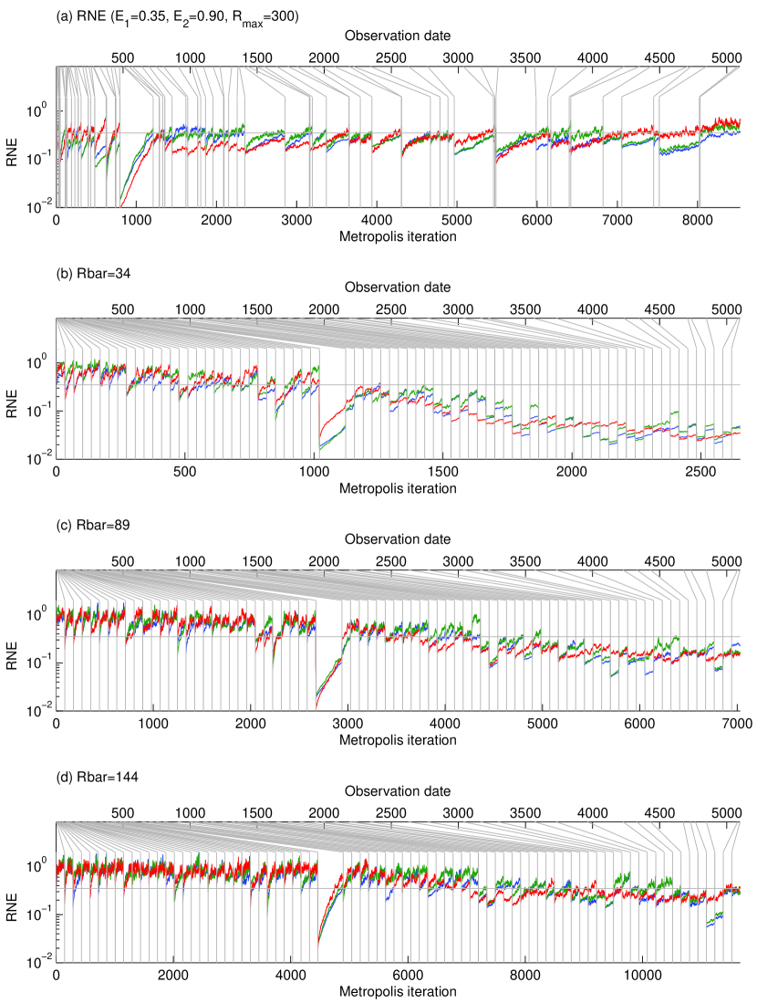
Figure 1: RNE of test functions at each Metropolis iteration: (a) RNE-based stopping rule; (b) $\overline{R}=34$; (c) $\overline{R}=89$; (d) $\overline{R}=144$.

Figure 1 shows RNE for all three test functions $g_{i}(\theta,y_{1:t_{\ell}})$ at each Metropolis iteration of each cycle $\ell$. The figure reports results for four different $M$ phase stopping rules: the RNE-based rule (with $E_{1}=0.35$, $E_{2}=0.90$ and $R_{\text{max}}=300$) and the deterministic rule with $\overline{R}$ = 34, 89 and 144. The beginning of each $M$ phase is indicated by a vertical line. The lower axis of each panel indicates the Metropolis iteration (cumulating across cycles); the top axis indicates the observation date $t$ at which each $M$ phase takes place; and the left axis indicates RNE. For reference, Figure 1 includes a horizontal line indicating $\textit{RNE}=0.35$. This is the default target for the RNE-based stopping rule and serves as a convenient benchmark for the other rules as well.

In the early part of the sample, the deterministic rules execute many more Metropolis steps than needed to achieve the nominal target of $\textit{RNE}=0.35$. However, these require relatively little time because sample size $t$ is small. As noted above, there is little point in undertaking additional Metropolis iterations once RNE approaches one, as happens toward the beginning of the sample for all three deterministic rules shown in the figure.

Toward the end of the sample, achieving any fixed RNE target in the $M$ phase requires more iterations due to the extreme non-Gaussianity of the posterior (see Section 5.4 for a more detailed discussion of this issue). The RNE-based rule adapts automatically, performing iterations only as needed to meet the RNE target, implying more iterations as sample size increases in this application.

At observation $t=474$, November 15, 1991, the $C$ phase terminates with very low RSS (regardless of $M$ phase stopping rule used), the result of a return that is highly unlikely conditional on the model and past history of returns. The deterministic rules undertake additional Metropolis iterations to compensate, as detailed in Section 3.3. The RNE-based rule also requires more iterations than usual to meet the relevant threshold; but in this case the number of additional iterations undertaken is determined algorithmically.

Table 4: Moment approximations

		10 $\times$ Volatility State					1000 $\times$ (3% Loss Probability)					10 $\times$ Skewness
$\overline{R}$	Compute	E	SD	NSE	RNE		E	SD	NSE	RNE		E	SD	NSE	RNE
	Time
March 31, 2009
5	91	-37.405	0.373	0.027	0.003		95.877	7.254	0.513	0.003		-1.999	0.823	0.063	0.003
8	127	-37.388	0.390	0.029	0.003		96.457	7.543	0.531	0.003		-2.204	0.837	0.060	0.003
13	205	-37.347	0.366	0.020	0.005		97.311	7.167	0.361	0.006		-2.348	0.774	0.034	0.008
21	304	-37.382	0.352	0.014	0.009		96.767	6.938	0.255	0.011		-2.530	0.788	0.030	0.011
34	482	-37.339	0.349	0.011	0.015		97.582	6.913	0.211	0.016		-2.569	0.812	0.021	0.023
55	776	-37.340	0.353	0.007	0.034		97.591	6.970	0.142	0.037		-2.563	0.811	0.011	0.079
89	1245	-37.330	0.364	0.006	0.055		97.735	7.133	0.109	0.065		-2.574	0.812	0.010	0.105
144	2120	-37.332	0.355	0.004	0.141		97.743	6.996	0.066	0.172		-2.580	0.816	0.007	0.230
	2329	-37.334	0.359	0.003	0.170		97.687	7.037	0.063	0.192		-2.587	0.818	0.005	0.406
March 31, 2010
5	91	-50.563	0.309	0.014	0.007		0.596	0.253	0.013	0.006		-2.078	0.816	0.063	0.003
8	127	-50.514	0.309	0.011	0.012		0.662	0.276	0.013	0.007		-2.274	0.838	0.059	0.003
13	205	-50.517	0.309	0.009	0.016		0.696	0.284	0.010	0.013		-2.425	0.771	0.033	0.008
21	304	-50.512	0.310	0.007	0.031		0.736	0.295	0.008	0.021		-2.599	0.780	0.028	0.012
34	482	-50.492	0.309	0.006	0.044		0.754	0.301	0.006	0.045		-2.616	0.795	0.018	0.030
55	776	-50.491	0.310	0.004	0.097		0.755	0.302	0.004	0.103		-2.610	0.797	0.010	0.093
89	1245	-50.482	0.315	0.003	0.164		0.765	0.308	0.003	0.162		-2.640	0.794	0.008	0.145
144	2120	-50.483	0.314	0.002	0.381		0.765	0.308	0.002	0.240		-2.632	0.800	0.006	0.276
	2329	-50.482	0.315	0.002	0.460		0.769	0.307	0.002	0.588		-2.643	0.796	0.005	0.452

Table 4 reports details on the posterior mean approximations for the two dates of interest. Total computation time for running the simulator across the full sample is provided for reference. The last line in each panel, indicated by ‘*’ in the $\overline{R}$ field, uses the RNE-based stopping rule. For both dates, the NSE of the approximation declines substantially as $\overline{R}$ increases. Comparison of the compute times reported in Table 4 again suggests that increasing $\overline{R}$ is more efficient for reducing NSE than would be increasing $N$, up to at least $\overline{R}=89$.

Some bias in the moment approximations is evident with low values of $\overline{R}$. The issue is most apparent for the 3% loss probability on March 31, 2010. Since volatility is low on that date, the probability of realizing a 3% loss is tiny and arises from tails of the posterior distribution of $\theta$, which is poorly represented in small samples. For example, with $\overline{R}=13$, RNE is 0.013, implying that each group of size $N=1024$ has an effective sample size of only about 13 particles. There is no evidence of bias for $\overline{R}\geq 89$ or with the RNE-based rule.

Plots such as those shown in Figure 1 provide useful diagnostics and are provided as a standard output of the software. For example, it is easy to see that with $\overline{R}=34$ (panel (b) of the figure) not enough iterations are performed in the $M$ phases, resulting in low RNE toward the end of the sample. With lower values of $\overline{R}$ the degradation in performance is yet more dramatic. As $\overline{R}$ is increased to 89 and 144 in panels (c) and (d) of the figure, respectively, the algorithm is better able to maintain particle diversity through the entire sample. The RNE-based rule does a good job at choosing an appropriate number of iterations in each $M$ phase and does so without the need for user input or experimentation.

5.4 Robustness to irregular posterior distributions

In the egarch_23 model there are 2 permutations of the factors $v_{kt}$ and 6 permutations of the components of the normal mixture probability distribution function of $\varepsilon_{t}$. This presents a severe challenge for single-chain MCMC as discussed by Celeux et al. (2000) and Jasra et al. (2007), and for similar reasons importance sampling is also problematic. The problem can be mitigated (Frühwirth-Schnatter, 2001) or avoided entirely (Geweke, 2007) by exploiting the special “mirror image” structure of the posterior distribution. But these models are still interesting as representatives of multimodal and ill-behaved posterior distributions in the context of generic posterior simulators. We focus here on the 6 permutations of the normal mixture in egarch_23.

Consider a $9\times 1$ parameter subvector $\psi$ with three distinct values of the triplets $\left(p_{s},\mu_{s},\sigma_{s}\right)$ $\left(s=A,B,C\right)$. There are six distinct ways in which these values could be assigned to components $i=1,2,3$ of the normal mixture (26) in the egarch_23 model. These permutations define six points $\psi_{u}$ $\left(u=1,\ldots,6\right)$. For all sample sizes $t$, the posterior densities $p\left(\psi_{u}\mid y_{1:t}\right)$ at these six points are identical. Let $\psi^{\prime}$ be a different parameter vector with analogous permutations $\psi^{\prime}_{u}$ $(u=1,\dots,6)$. As the sample adds evidence $p\left(\psi_{u}\mid y_{1:t}\right)/p\left(\psi_{u^{\prime}}\mid y_{1:t}\right)\overset{as}{\rightarrow}0$ or $p\left(\psi_{u}\mid y_{1:t}\right)/p\left(\psi_{u^{\prime}}\mid y_{1:t}\right)\overset{as}{\rightarrow}\infty$. Thus, a specific triplet set of triplets $\left(p_{s},\mu_{s},\sigma_{s}\right)$ $(s=A,B,C)$ and its permutations will emerge as pseudo-true values of the parameters (Geweke, 2005, Section 3.4).

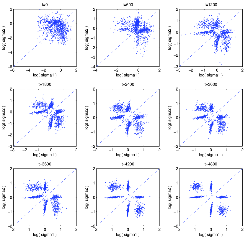
Figure 2: Scatterplots of a subset of particles $\left(\log\sigma_{1},\log\sigma_{2}\right)$ from selected posterior distributions conditional on $y_{1:t}$ ($J=64$, $N=4096$, $D_{1}=0.5$, $D_{2}=0.2$, $\overline{R}=34$).

The marginal distributions will exhibit these properties as well. Consider the pair $\left(\sigma_{1},\sigma_{2}\right)$, which is the case portrayed in Figure 2. The scatterplot is symmetric about the axis $\sigma_{1}=\sigma_{2}$ in all cases. As sample size $t$ increases six distinct and symmetric modes in the distribution gradually emerge. These reflect the full marginal posterior distribution for the normal mixture components of the egarch_23 model (i.e., marginalizing on all other parameters) that is roughly centered on the components $\left(p=0.17,\ \mu=0.16,\ \sigma=0.40\right)$, $\left(p=0.85,\ \mu=0.01,\ \sigma=1.01\right)$ and $\left(p=0.01,\ \mu=-1.36,\ \sigma=1.96\right)$. The progressive decrease in entropy with increasing $t$ illustrates how the algorithm copes with ill-behaved posterior distributions. Particles gradually migrate toward concentrations governed by the evidence in the sample. Unlike MCMC there is no need for particles to migrate between modes, and unlike importance sampling there is no need to sample over regions eliminated by the data (on the one hand) or to attempt to construct multimodal source distributions (on the other).

Similar phenomena are also evident for the other mixture parameters as well as for the parameters of the GARCH factors. The algorithm proposed in this paper adapts to these situations without specific intervention on a case-by-case basis.

5.5 Comparison with Markov chain Monte Carlo

To benchmark the performance of the algorithm against a more conventional approach, we constructed a straightforward Metropolis random walk MCMC algorithm, implemented in C code on a recent vintage CPU using the egarch_23 model. The variance matrix was tuned manually based on preliminary simulations, which required several hours of investigator time and computing time. The algorithm required 12,947 seconds for 500,000 iterations. The numerical approximation of the moment of interest $1000\cdot\operatorname{E}\left[P\left(Y_{t+1}<-0.03\mid y_{1:t},\theta\right)\right]$ for March 31, 2010, the same one addressed in Table 4, produced the result $0.763$ and a NSE of $0.003$. Taking the square of NSE to be inversely proportional to the number of MCMC iterations, an NSE of $0.002$ (the result for the RNE-based stopping rule in Table 4) would require about 1,840,000 iterations and 47,600 seconds computing time. Thus posterior simulation for the full sample would require about 20 times as long using random walk Metropolis in a conventional serial computing environment.

Although straightforward, this analysis severely understates the advantage of the sequential posterior simulator developed in this paper relative to conventional approaches. The MCMC simulator does not traverse all six mirror images of the posterior density. This fact greatly complicates attempts to recover marginal likelihood from the MCMC simulator output; see Celeux et al. (2000). To our knowledge the only reliable way to attack this problem using MCMC is to compute predictive likelihoods from the prior distribution and the posterior densities $p\left(\theta\mid y_{1:t}\right)$ $\left(t=1,\ldots,T-1\right)$. Recalling that $T=5100$, and taking computation time to be proportional to sample size (actually, it is somewhat greater) yields a time requirement of $2550\times 28167=71,825,850$ seconds (2.28 CPU years), which is almost 100,000 times as long as was required in the algorithm and implementation used here. Unless the function of interest $g(\theta,y_{1:T})$ is invariant to label switching (Geweke, 2007), the MCMC simulator must traverse all the mirror images with nearly equal frequency. As argued in Celeux et al. (2000), for all practical purposes this condition cannot be met with any reliability even with a simulator executed for several CPU centuries.

This example shows that simple “speedup factors” may not be useful in quantifying the reduction in computing time afforded by massively parallel computing environments. For the scope of models set in this work—that is, those satisfying Conditions 1 through 4—sequential posterior simulation is much faster than posterior simulation in conventional serial computing environments. This is a lower bound. There are a number of routine and reasonable objectives of posterior simulation, like those described in this section, that simply cannot be achieved at all with serial computing but are fast and effortless with SMC. Most important, sequential posterior simulation in a massively parallel computing environment conserves the time, energy and talents of the investigator for more substantive tasks.

6 Conclusion

Recent innovations in parallel computing hardware and associated software provide the opportunity for dramatic increases in the speed and accuracy of posterior simulation. Widely used MCMC simulators are not generically well-suited to this environment, whereas alternative approaches like importance sampling are. The sequential posterior simulator developed here has attractive properties in this context: inherent adaptability to new models; computational efficiency relative to alternatives; accurate approximation of marginal and predictive likelihoods; reliable and well-grounded measures of numerical accuracy; robustness to irregular posteriors; and a well-developed theoretical foundation. Establishing these properties required a number of contributions to the literature, summarized in Section 1 and then developed in Sections 2, 3 and 4. Section 5 provided an application to a state-of-the-art model illustrating the properties of the simulator.

The methods set forth in the paper reduce computing time dramatically in a parallel computing environment that is well within the means of academic investigators. Relevant comparisons with conventional serial computing environments entail different algorithms, one for each environment. Moreover, the same approximation may be relatively more advantageous in one environment than the other. This precludes generic conclusions about “speed-up factors.” In the example in Section 5, for a simple posterior moment, the algorithm detailed in Section 3.3 was nearly 10 times faster than a competing random-walk Metropolis simulator in a conventional serial computing environment. For predictive likelihoods and marginal likelihood it was 100,000 times faster. The parallel computations used a single graphics processing unit (GPU). Up to eight GPU’s can be added to a standard desktop computer at a cost ranging from about $350 (US) for a mid-range card to about $2000 (US) for a high-performance Tesla card. Computation time is inversely proportional to the number of GPU’s.

These contributions address initial items on the research agenda opened up by the prospect of massively parallel computing environments for posterior simulation. In the near term it should be possible to improve on the specific contribution made here in the form of the algorithm detailed in Section 3.3. Looking forward on the research agenda, a major component is extending the class of models for which generic sequential posterior simulation will prove practical and reliable. Large-scale hierarchical models, longitudinal data, and conditional data density evaluations that must be simulated all pose fertile ground for future work.

The research reported here has been guided by two paramount objectives. One is to provide methods that are generic and minimize the demand for knowledge and effort on the part of applied statisticians who, in turn, seek primarily to develop and apply new models. The other is to provide methods that have a firm methodological foundation whose relevance is borne out in subsequent applications. It seems to us important that these objectives should be central in the research agenda.

References

Andrieu C, Doucet A, Holenstein A (2010). Particle Markov chain Monte Carlo. Journal of the Royal Statistical Society, Series B 72: 1–33.

Baker JE (1985). Adaptive selection methods for genetic algorithms. In Grefenstette J (ed.), Proceedings of the International Conference on Genetic Algorithms and Their Applications, 101–111. Malwah NJ: Erlbaum.

Baker JE (1987). Reducing bias and inefficiency in the selection algorithm. In Grefenstette J (ed.) Genetic Algorithms and Their Applications, 14–21. New York: Wiley.

Berkowitz, J (2001). Testing density forecasts with applications to risk management. Journal of Business and Economic Statistics 19: 465–474.

Carpenter J, Clifford P, Fearnhead P (1999). Improved particle filter for nonlinear problems. IEEE Proceedings – Radar Sonar and Navigation 146: 2–7.

Celeux G, Hurn M, Robert CP (2000). Computational and inferential difficulties with mixture posterior distributions. Journal of the American Statistical Association 95: 957–970.

Chopin N (2002). A sequential particle filter method for static models. Biometrika 89: 539–551.

Chopin N (2004). Central limit theorem for sequential Monte Carlo methods and its application to Bayesian inference. Annals of Statistics 32: 2385–2411.

Chopin N, Jacob P (2010). Free energy sequential Monte Carlo, application to mixture modelling. In: Bernardo JM, Bayarri MJ, Berger JO, Dawid AP, Heckerman D, Smith AFM, West M (eds.), Bayesian Statistics 9. Oxford: Oxford University Press.

Chopin N, Jacob PI, Papaspiliopoulis O (2011). SMC²: A sequential Monte Carlo algorithm with particle Markov chain Monte Carlo updates. Working paper. http://arxiv.org/PS_cache/arxiv/pdf/1101/1101.1528v2.pdf

Del Moral P, Doucet A, Jasra A (2006). Sequential Monte Carlo samplers. Journal of the Royal Statistical Society, Series B 68: 411–436.

Del Moral P, Doucet A, Jasra A (2011). On adaptive resampling strategies for sequential Monte Carlo methods. Bernoulli, forthcoming.

Diebold FX, Gunther TA, Tay AS. (1998). Evaluating density forecasts with applications to financial risk management. International Economic Review 39: 863–883.

Douc R, Moulines E (2008). Limit theorems for weighted samples with applications to sequential Monte Carlo methods. The Annals of Statistics 36: 2344–2376.

Durham G, Geweke J (2011). Massively parallel sequential Monte Carlo for Bayesian inference. Working paper. http://www.censoc.uts.edu.au/pdfs/geweke_papers/gp_working_9.pdf

Durham G, Geweke J (2013). Improving asset price prediction when all models are false. Journal of Financial Econometrics, forthcoming.

Fearnhead P (1998). Sequential Monte Carlo methods in filter theory. Ph.D. thesis, Oxford University.

Flegal JM, Jones GL (2010). Batch means and spectral variance estimates in Markov chain Monte Carlo. Annals of Statistics 38: 1034–1070.

Frühwirth-Schnatter S (2001). Markov chain Monte Carlo estimation of classical and dynamic switching and mixture models. Journal of the American Statistical Association 96: 194–209.

Fulop A, Li J (2011). Robust and efficient learning: A marginalized resample-move approach. Working paper. http://papers.ssrn.com/sol3/papers.cfm?abstract_id=1724203

Gelman A, Roberts, GO, Gilks, WR (1996). Efficient Metropolis jumping rules. In: Bernardo JM, Berger JO, Dawid AP, Smith AFM (eds.), Bayesian Statistics 5. Oxford: Oxford University Press.

Geweke J (1989). Bayesian inference in econometric models using Monte Carlo integration. Econometrica 57: 1317–1340.

Geweke J (2005). Contemporary Bayesian Econometrics and Statistics. Englewood Cliffs NJ: Wiley.

Geweke J (2007). Interpretation and inference in mixture models: simple MCMC works. Computational Statistics and Data Analysis 51: 3529–3550.

Geweke J, Amisano G (2010). Comparing and evaluating Bayesian predictive distributions of asset returns. International Journal of Forecasting 26: 216–230.

Geweke J, Durham G, Xu H (2013). Bayesian inference for logistic regression models using sequential posterior simulation. http://www.business.uts.edu.au/economics/staff/jgeweke/Geweke_Durham_XU_2013.pdf

Gilks WR, Berzuini C (2001). Following a moving target – Monte Carlo inference for dynamic Bayesian models. Journal of the Royal Statistical Society, Series B 63: 127–146.

Gordon NG, Salmond DG, Smith AFM (1993). A novel approach to non-linear and non-Gaussian Bayesian state estimation. IEEE Proceedings F: Radar and Signal Processing 140: 107–113.

Hendeby G, Karlsson R, Gustafsson F (2010). Particle filtering: The Need for Speed. EURASIP Journal on Advances in Signal Processing doi:10.1155/2010/181403

Herbst E, Schorfheide F (2012). Sequential Monte Carlo Sampling for DSGE Models. Unpublished working paper.

Innovative Computing Laboratory (ICL), University of Tennessee (2013). Matrix Algebra for GPU and Multicore Architectures. http://icl.cs.utk.edu/magma/

Jasra A, Stephens DA, Holmes CC (2007). On population-based simulation for static inference. Statistics and Computing 17: 263–279.

Kitagawa, G (1996). Monte Carlo filter and smoother for non-Gaussian nonlinear state space models. Journal of Computational and Graphical Statistics 5: 1–25.

Kloek T, van Dijk HK (1978). Bayesian estimates of equation system parameters: An application of integration by Monte Carlo. Econometrica 46:1–19.

Kong A, Liu JS, Wong WH (1994). Sequential imputations and Bayesian missing data problems. Journal of the American Statistical Association 89: 278–288.

Lee L, Yau C, Giles MB, Doucet A, Homes CC (2010). On the utility of graphics cards to perform massively parallel simulation of advanced Monte Carlo Methods. Journal of Computational and Graphical Statistics 19: 769–789.

Liu JS, Chen R (1995). Blind deconvolution via sequential imputations. Journal of the American Statistical Association 90: 567–576.

Liu JS, Chen R (1998). Sequential Monte Carlo methods for dynamic systems. Journal of the American Statistical Association 93: 1032–1044.

Matlab (2013). Matlab Parallel Computing Toolbox. http://www.mathworks.com/products/parallel-computing/description5.html

McGrayne SHB (2011). The Theory that Would Not Die: How Bayes’ Rule Cracked the Enigma Code, Hunted Down Russian Submarines, and Emerged Triumphant from Two Centuries of Controversy. New Haven: Yale University Press.

Nelson DB (1991). Conditional heteroskedasticity in asset returns: A new approach. Econometrica 59: 347–370.

Nvidia (2013). Nvidia CUDA C Programming Guide, Version 5.0. http://docs.nvidia.com/cuda/pdf/CUDA_C_Programming_Guide.pdf

Rosenblatt, M (1952). Remarks on a multivariate transformation. Annals of Mathematical Statistics 23: 470–472.

Smith, JQ (1985). Diagnostic checks of non-standard time series models. Journal of Forecasting 4: 283–291.

Souchard MA, Wang Q, Chan C, Frelinger J, Cron A, West M (2010). Understanding GPU programming for statistical computation: Studies in Massively parallel massive mixtures. Journal of Computational Graphics and Statistics 19: 419–438.

Tierney L (1994). Markov chains for exploring posterior distributions (with discussion and rejoinder). Annals of Statistics 22: 1701–1762.