11institutetext: Caio H. Lewenkopf 22institutetext: Instituto de Física, Universidade Federal Fluminense, Brazil
22email: caio@if.uff.br
33institutetext: Eduardo R. Mucciolo 44institutetext: Department of Physics, University of Central Florida, USA
44email: mucciolo@physics.ucf.edu

The recursive Green’s function method for graphene

Caio H. Lewenkopf    Eduardo R. Mucciolo
(Received: date / Accepted: date)
Abstract

We describe how to apply the recursive Green’s function method to the computation of electronic transport properties of graphene sheets and nanoribbons in the linear response regime. This method allows for an amenable inclusion of several disorder mechanisms at the microscopic level, as well as inhomogeneous gating, finite temperature, and, to some extend, dephasing. We present algorithms for computing the conductance, density of states, and current densities for armchair and zigzag atomic edge alignments. Several numerical results are presented to illustrate the usefulness of the method.

Keywords:
electronic transport recursive Green’s function method graphene nanoribbons
pacs:
73.23.-b 72.80.Vp 81.05.ue

1 Introduction

Since graphene was first produced, several synthesis strategies have been put forward. Significant progress has been made to produce better quality samples with the goal of improving their transport properties. Despite the enormous effort, we are still very far from reaching the perfect ballistic regime and disorder always plays a central role, particularly in electronic transport. Disorder appears in several different forms, being either local (such as lattice defects, edge irregularities, and surface adsorbates) or long ranged (such as charge impurities trapped in the substrate or ripples due to substrate roughness) CastroNeto09 .

Several theoretical methods have been developed to describe electronic transport in disordered graphene Mucciolo10 . The effective low-energy Dirac Hamiltonian, derived from band-structure theory, combined with a standard diagrammatic perturbative expansion is an excellent analytical tool for giving us insight into the properties of disordered graphene Shon98 ; Ostrovsky06 . However, it has (kF)1superscriptsubscript𝑘𝐹1(k_{F}\ell)^{-1} as a small expansion parameter, where kFsubscript𝑘𝐹k_{F} stands for the Fermi wave number and \ell is the electron mean free path. Thus, it describes well the conductivity in graphene at high doping, but becomes of limited use when one is interested in the physics close to the charge neutrality point, where kF1much-less-thansubscript𝑘𝐹1k_{F}\ell\ll 1. Theoretical investigations of the that regime require instead the use of numerical methods.

Most numerical methods employed to study the transport properties of disordered graphene use an atomistic basis Mucciolo10 . The few exceptions are tailor-made methods to deal with long-range disorder, where either a momentum representation Nomura07 ; Nomura07b or discretized version of the Dirac equation Tworzydlo08 ; Hernandez12 are used within a single-valley approximation.

For many applications, one is interested in the two- or multiple-probe conductance. For the conductance, differently from the conductivity, geometry plays an important role. The recursive Green’s function (RGF) method Thouless81 became the standard tool to compute transport properties in this case. The method is very reliable, computationally efficient, and allows for a parallel implementation Drouvelis06 . It can model arbitrary geometries and efficiently addresses a variety of scattering processes within the single-particle approximation. The goal of this paper is to show how to compute electronic transport properties of graphene samples within the tight-binding approximation using the RGF method. The key element is an efficient algorithm for evaluating the single-particle Green’s function of sheets or ribbons.

The recursive method was developed by Thouless and Kirkpatrick Thouless81 for computing the linear electronic conductance of linear atomic chains in the presence of on-site disorder. The method was later generalized to two-dimensional systems in the “slice” formulation, which is the form most used nowadays MacKinnon85 . Variations of the method have been introduced in the literature to treat three-dimensional Sols89 and multi-probe systems Baranger91 with arbitrary geometries, see e.g. Ref. Kazymyrenko08 .

We note that other efficient, atomistic methods have been employed in recent years to study electronic transport in mesoscopic systems: For instance, the wave-packet time evolution Kramer10 ; Yuan10 , the kernel polynomial expansion Weisse06 ; Ferreira11 , and the continued fraction expansion Triozon05 , to name a few. Recently, an alternative method to compute transport of ballistic graphene junctions, particularly effective when strong magnetic fields are presented, was introduced Liu2012 . However, for most practitioners, the RGF remains the best method for tackling large-scale but finite-size problems where quantum coherence and disorder are present simultaneously.

This paper does not attempt to be a comprehensive review of the recursive method, but rather a self-contained description that gives to interested readers, yet unfamiliar with the RGF method, all the basic material necessary to implement a calculation on their own. For that purpose, we briefly present some standard material covered in textbooks Datta96 ; Ferry97 , discuss some more advanced issues which are found scattered in the literature, and present original developments tailor-made for graphene.

This paper is organized as follows. We begin by quickly reviewing some fundamental relations of electronic transport theory and by providing the essential formulation of the method. In Sec. 3 we present the recursive Green’s function method. The method requires as input the surface Green’s functions of the electronic leads, taken at the lead-device interface. In Sec. 4 we describe how to compute the surface Green’s function of semi-infinite lattices that play the role of leads. Next, we present an efficient discretization scheme to implement the recursive method for graphene sheets and nanoribbons. In Sec. 6 we show how to evaluate quantities such as the local density of states and local current densities. Very often, one is interested in cases where the coherence length ϕsubscriptitalic-ϕ\ell_{\phi} is comparable to the system size L𝐿L. For such situations, it is possible to account for dephasing using the phenomenological voltage probe model, as described in Sec. 7. In the context of graphene, the main application of the RGF method is the study of disorder effects in electronic transport. We discuss the main kinds of disorder and show how to account for them in Sec. 8. We conclude by presenting a number of numerical results that illustrate the method in Sec. 9.

2 Elements of Linear Mesoscopic Transport

In this Section we review the key elements necessary to implement the recursive Green’s function method for two-dimensional systems. The linear dc conductance is computed using the exact single-particle retarded Green’s function that connects the source and drain leads, in conjunction with either the Landauer Landauer88 or the Caroli formula Caroli71 .

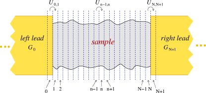
For a two-probe setup, as illustrated by Fig. 1, the zero-temperature linear conductance is given by the Landauer formula

𝒢=2e2hTrc[tt].𝒢2superscript𝑒2subscriptTr𝑐delimited-[]superscript𝑡𝑡{\cal G}=\frac{2e^{2}}{h}{\rm Tr}_{c}\left[t^{\dagger}t\right]. (1)

Here, t(t)𝑡superscript𝑡t(t^{\prime}) is the transmission matrix across the system from left to right (right to left) and r(r)𝑟superscript𝑟r(r^{\prime}) is the reflection matrix at the left-hand (right-hand) side. The factor of 2 stands for spin degeneracy and the trace is taken over the propagating modes at the left and right leads. The transmission matrix can be obtained from the S𝑆S matrix,

S=(rttr),𝑆𝑟superscript𝑡𝑡superscript𝑟S=\left(\begin{array}[]{cc}r&t^{\prime}\\ t&r^{\prime}\end{array}\right), (2)

which is given by Lee81 ; Fisher81

Sab(E)=subscript𝑆𝑎𝑏𝐸absent\displaystyle S_{ab}(E)= δab+ivavbsubscript𝛿𝑎𝑏𝑖Planck-constant-over-2-pisubscript𝑣𝑎subscript𝑣𝑏\displaystyle-\delta_{ab}+i\hbar\sqrt{v_{a}v_{b}}
×dyqdypχa(yq)Gr(yq,yp;E)χb(yp),\displaystyle\;\;\;\times\int\!dy_{q}\int\!dy_{p}\,\chi_{a}^{*}(y_{q})G^{r}(y_{q},y_{p};E)\chi_{b}(y_{p}), (3)

where vcsubscript𝑣𝑐v_{c} and χc(yp)subscript𝜒𝑐subscript𝑦𝑝\chi_{c}(y_{p}) are, respectively, the longitudinal propagation velocity and its transverse wave function in the propagating channel c𝑐c of lead p𝑝p (either on the left-hand or right-hand side). The integrations run over the contact regions at the right and left terminations of the graphene sheet (see Fig. 1). The key element in Eq. (2) is Gr(yq,yp;E)superscript𝐺𝑟subscript𝑦𝑞subscript𝑦𝑝𝐸G^{r}(y_{q},y_{p};E), the retarded Green’s function corresponding to an electron with energy E𝐸E propagating from positions ypsubscript𝑦𝑝y_{p} to yqsubscript𝑦𝑞y_{q}.

Refer to caption
Figure 1: Typical two-probe scheme used in the numerical calculations: The sample is described by G(yq,yp;E)𝐺subscript𝑦𝑞subscript𝑦𝑝𝐸G(y_{q},y_{p};E). The perfect leads can be accounted for by either propagating mode wave functions χcsubscript𝜒𝑐\chi_{c} and their density of states ρcsubscript𝜌𝑐\rho_{c} (Landauer formula) or by level widths ΓΓ\Gamma (Caroli formula).

The recursive Green’s function method reviewed in this paper is an efficient tool to compute the scattering properties of noninteracting electrons described by a tight-binding Hamiltonian of the form

H=ij(tij|ij|+H.c)+iVi|ii|.H=-\sum_{i\neq j}\left(t_{ij}|i\rangle\langle j|+{\rm H.c}\right)+\sum_{i}V_{i}|i\rangle\langle i|. (4)

In graphene, the hopping terms tijsubscript𝑡𝑖𝑗t_{ij} typically connect only nearest neighbor sites i𝑖i and j𝑗j of a honeycomb lattice (single-orbital approximation), although it is straightforward to include next-to-nearest hopping terms as well, if required. The model can account for an external magnetic field by a suitable modification of the hopping terms, as shown in Appendix B. Here, Visubscript𝑉𝑖V_{i} stands for a local potential due to gating or disorder.

For simplicity, here we consider only tight-binding models with orthogonal orbitals and nearest-neighbor hopping terms. The computational cost of the RGF method scales as N×M3𝑁superscript𝑀3N\times M^{3}, where N𝑁N is the number of slices and M𝑀M is the typical number of sites in a given slice, see Fig. 1. The RGF implementation scheme presented in this paper is particularly recommended when the system’s translational invariance is broken by disorder and/or an irregular geometry. For systems with translational invariance at the transverse direction, it can be advantageous to work in the k𝑘k-space and use alternative hybrid RGF implementations (such as in Ref. Sajjad13 ) or other methods, e.g. Ref. Liu2012 .

In the tight-binding basis, Eq. (2) reads

Sab(E)=δab+ivavba0ipjqχa(i)Gqpr(i,j)χb(j),subscript𝑆𝑎𝑏𝐸subscript𝛿𝑎𝑏𝑖Planck-constant-over-2-pisubscript𝑣𝑎subscript𝑣𝑏subscript𝑎0subscript𝑖𝑝subscript𝑗𝑞superscriptsubscript𝜒𝑎𝑖subscriptsuperscript𝐺𝑟𝑞𝑝𝑖𝑗subscript𝜒𝑏𝑗S_{ab}(E)=-\delta_{ab}+i\hbar\frac{\sqrt{v_{a}v_{b}}}{a_{0}}\sum_{i\in p}\sum_{j\in q}\chi_{a}^{*}(i)G^{r}_{qp}(i,j)\chi_{b}(j), (5)

where the sums run over the sites at the contacts p𝑝p and q𝑞q where the propagating channels a𝑎a and b𝑏b are defined, respectively. Notice that in two spatial dimensions

χa(yp)1a0χa(i)=1a0i|χasubscript𝜒𝑎subscript𝑦𝑝1subscript𝑎0subscript𝜒𝑎𝑖1subscript𝑎0inner-product𝑖subscript𝜒𝑎\displaystyle\chi_{a}(y_{p})\rightarrow\frac{1}{\sqrt{a_{0}}}\chi_{a}(i)=\frac{1}{\sqrt{a_{0}}}\langle i|\chi_{a}\rangle (6)
and
Gr(yq,yp)1a02Gqpr(j,i),superscript𝐺𝑟subscript𝑦𝑞subscript𝑦𝑝1superscriptsubscript𝑎02subscriptsuperscript𝐺𝑟𝑞𝑝𝑗𝑖\displaystyle G^{r}(y_{q},y_{p})\rightarrow\frac{1}{a_{0}^{2}}G^{r}_{qp}(j,i), (7)

where a0subscript𝑎0a_{0} is the lattice constant. Let us consider the case where the leads are modeled by semi-infinite square lattices. One can then introduce the level widths Datta96

Γp(i,i)=aχa(i)vaa0χa(i).subscriptΓ𝑝𝑖superscript𝑖subscript𝑎subscript𝜒𝑎𝑖Planck-constant-over-2-pisubscript𝑣𝑎subscript𝑎0subscript𝜒𝑎superscript𝑖\Gamma_{p}(i,i^{\prime})=\sum_{a}\chi_{a}(i)\frac{\hbar v_{a}}{a_{0}}\chi_{a}(i^{\prime}). (8)

It is straightforward to show that, in this case,

Trc[tt]=i,iLj,jRΓL(i,i)GLRr(i,j)ΓR(j,j)GRLa(j,i)=𝒯subscriptTr𝑐delimited-[]𝑡superscript𝑡subscriptFRACOP𝑖superscript𝑖𝐿𝑗superscript𝑗𝑅subscriptΓ𝐿𝑖superscript𝑖subscriptsuperscript𝐺𝑟𝐿𝑅superscript𝑖𝑗subscriptΓ𝑅𝑗superscript𝑗subscriptsuperscript𝐺𝑎𝑅𝐿superscript𝑗𝑖𝒯\mbox{Tr}_{c}\left[tt^{\dagger}\right]=\sum_{{i,i^{\prime}\in L}\atop{j,j^{\prime}\in R}}\Gamma_{L}(i,i^{\prime})G^{r}_{LR}(i^{\prime},j)\Gamma_{R}(j,j^{\prime})G^{a}_{RL}(j^{\prime},i)={\cal T} (9)

where

𝒯Trs[ΓLGLRrΓRGRLa].𝒯subscriptTr𝑠delimited-[]subscriptΓ𝐿superscriptsubscript𝐺𝐿𝑅𝑟subscriptΓ𝑅superscriptsubscript𝐺𝑅𝐿𝑎{\cal T}\equiv\mbox{Tr}_{s}\Big{[}\Gamma_{L}G_{LR}^{r}\Gamma_{R}G_{RL}^{a}\Big{]}. (10)

Here, the subscript in the trace indicates whether the sums run over channels (c𝑐c) or sites (s𝑠s). Depending on the author, the expression on the r.h.s. of Eq. (9) is called either Caroli Caroli71 or Meir-Wingreen Meir92 conductance formula.

This demonstration of the equivalence between the Landauer and Caroli formulas relies on the Fisher and Lee S𝑆S-matrix and on an expression for ΓpsubscriptΓ𝑝\Gamma_{p} which is only suitable for a square lattice. This derivation is simple and to some extend non rigorous but captures the essential elements that will be discussed in what follows, namely, the Green’s functions GRL(r,a)subscriptsuperscript𝐺𝑟𝑎𝑅𝐿G^{(r,a)}_{RL} and the decay width matrices ΓR,LsubscriptΓ𝑅𝐿\Gamma_{R,L}. There are several ways to show that (9) holds in general in the linear response regime, see e.g. Ref. Hernandez07 .

When the full S𝑆S matrix is known, it is possible to obtain the global density of states through the Wigner time delay Lewenkopf08 , namely,

ρ(E)=i2πTrc(SSE),𝜌𝐸𝑖2𝜋subscriptTr𝑐superscript𝑆𝑆𝐸\rho(E)=-\frac{i}{2\pi}\mbox{Tr}_{c}\left(S^{\dagger}\frac{\partial S}{\partial E}\right), (11)

where the derivative of S𝑆S with respect to the energy can be done numerically. The computation of (11) is significantly less expensive than evaluating ρ(E)𝜌𝐸\rho(E) through the standard expression, namely,

ρ(E)=1πIm[TrsGr(E)],𝜌𝐸1𝜋Imdelimited-[]subscriptTrsuperscript𝑠superscript𝐺𝑟𝐸\rho(E)=-\frac{1}{\pi}\mbox{Im}\Big{[}\mbox{Tr}_{s^{\prime}}\,G^{r}(E)\Big{]}, (12)

but it requires the knowledge of the explicit form of the lead wave functions χa(i)subscript𝜒𝑎𝑖\chi_{a}(i). Note that, in Eq. (12), the trace is taken over all sites of the graphene sample.

The Fano factor is another quantity of interest Lewenkopf08 . It can be evaluated through the expression

F=1Trc[tttt]Trc[tt].𝐹1subscriptTr𝑐delimited-[]superscript𝑡𝑡superscript𝑡𝑡subscriptTr𝑐delimited-[]superscript𝑡𝑡F=1-\frac{{\rm Tr}_{c}\left[t^{\dagger}t\,t^{\dagger}t\right]}{{\rm Tr}_{c}\left[t^{\dagger}t\right]}. (13)

Notice that one can define left-to-right and right-to-left Fano factors, as in the case for the conductance, by switching the matrix t𝑡t with tsuperscript𝑡t^{\prime}. The Fano factor can be computed without an explicit knowledge of the wave functions χa(i)subscript𝜒𝑎𝑖\chi_{a}(i) by noticing that Eq. (13) can be recast as

F=1Trs[ΓLGLRrΓRGRLaΓLGLRrΓRGRLa]𝒯.𝐹1subscriptTr𝑠delimited-[]subscriptΓ𝐿superscriptsubscript𝐺𝐿𝑅𝑟subscriptΓ𝑅superscriptsubscript𝐺𝑅𝐿𝑎subscriptΓ𝐿superscriptsubscript𝐺𝐿𝑅𝑟subscriptΓ𝑅superscriptsubscript𝐺𝑅𝐿𝑎𝒯F=1-\frac{\mbox{Tr}_{s}\Big{[}\Gamma_{L}G_{LR}^{r}\Gamma_{R}G_{RL}^{a}\Gamma_{L}G_{LR}^{r}\Gamma_{R}G_{RL}^{a}\Big{]}}{\cal T}. (14)

Let us present the same basic expression in a more suitable form for the recursive calculations. We begin by writing the Caroli formula for the transmission probability at a given energy E𝐸E using the slice indexing,

𝒯=Trs[ΓLG0,N+1r(E)ΓRGN+1,0a(E)],𝒯subscriptTr𝑠delimited-[]subscriptΓ𝐿subscriptsuperscript𝐺𝑟0𝑁1𝐸subscriptΓ𝑅subscriptsuperscript𝐺𝑎𝑁10𝐸{\cal T}={\rm Tr}_{s}\left[\Gamma_{L}\,G^{r}_{0,N+1}(E)\,\Gamma_{R}\,G^{a}_{N+1,0}(E)\right], (15)

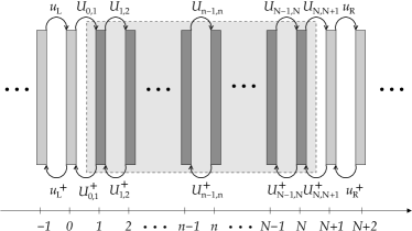
where Gr,asuperscript𝐺𝑟𝑎G^{r,a} are the retarded and advanced Green’s functions across the system (see Fig. 2 for a definition of the subscripts in terms of slice numbers). These Green’s functions are matrices whose rank is defined by the number of sites in the slices.111The number of sites per slice does not need to be equal for all slices. The level width matrices are given by the expression

ΓL,R=i[ΣL,Rr(E)ΣL,Rr(E)],subscriptΓ𝐿𝑅𝑖delimited-[]superscriptsubscriptΣ𝐿𝑅𝑟𝐸superscriptsubscriptΣ𝐿𝑅𝑟𝐸\Gamma_{L,R}=i\left[\Sigma_{L,R}^{r}(E)-\Sigma_{L,R}^{r\,\dagger}(E)\right], (16)

where the retarded surface self-energies of the leads read

ΣLr(E)=uLgLr(E)uLandΣRr(E)=uRgRr(E)uR.formulae-sequencesuperscriptsubscriptΣ𝐿𝑟𝐸subscript𝑢𝐿superscriptsubscript𝑔𝐿𝑟𝐸superscriptsubscript𝑢𝐿andsuperscriptsubscriptΣ𝑅𝑟𝐸superscriptsubscript𝑢𝑅superscriptsubscript𝑔𝑅𝑟𝐸subscript𝑢𝑅\Sigma_{L}^{r}(E)=u_{L}\,g_{L}^{r}(E)\,u_{L}^{\dagger}\quad\mbox{and}\quad\Sigma_{R}^{r}(E)=u_{R}^{\dagger}\,g_{R}^{r}(E)\,u_{R}. (17)

Notice that the retarded Green’s functions gLrsuperscriptsubscript𝑔𝐿𝑟g_{L}^{r} and gRrsuperscriptsubscript𝑔𝑅𝑟g_{R}^{r} are defined at the surface of the left and right leads, respectively, when the leads are decoupled from the system. They obey the self-consistent equations

[E+i0+hLΣLr(E)]gLr(E)=Ianddelimited-[]𝐸𝑖superscript0subscript𝐿subscriptsuperscriptΣ𝑟𝐿𝐸superscriptsubscript𝑔𝐿𝑟𝐸𝐼and\displaystyle\left[E+i0^{+}-h_{L}-\Sigma^{r}_{L}(E)\right]g_{L}^{r}(E)=I\quad\mbox{and}\quad
[E+i0+hRΣRr(E)]gRr(E)=I,delimited-[]𝐸𝑖superscript0subscript𝑅subscriptsuperscriptΣ𝑟𝑅𝐸superscriptsubscript𝑔𝑅𝑟𝐸𝐼\displaystyle\left[E+i0^{+}-h_{R}-\Sigma^{r}_{R}(E)\right]g_{R}^{r}(E)=I, (18)

where hLsubscript𝐿h_{L} and hRsubscript𝑅h_{R} are the Hamiltonians of isolated, individual slices in the left and right leads, respectively. The connection matrices uLsubscript𝑢𝐿u_{L} and uRsubscript𝑢𝑅u_{R} are defined to run from left-to-right and are assumed uniform inside the leads. If the leads are identical, then gRr=gLrsuperscriptsubscript𝑔𝑅𝑟superscriptsubscript𝑔𝐿𝑟g_{R}^{r}=g_{L}^{r}, hL=hRsubscript𝐿subscript𝑅h_{L}=h_{R}, uR=uLsubscript𝑢𝑅superscriptsubscript𝑢𝐿u_{R}=u_{L}^{\dagger}, ΣRr(E)=ΣLr(E)subscriptsuperscriptΣ𝑟𝑅𝐸subscriptsuperscriptΣ𝑟𝐿𝐸\Sigma^{r}_{R}(E)=\Sigma^{r}_{L}(E), and ΓR=ΓLsubscriptΓ𝑅subscriptΓ𝐿\Gamma_{R}=\Gamma_{L}. Notice that, in general, the coupling matrices are Hermitian, (ΓR,L)=ΓR,LsuperscriptsubscriptΓ𝑅𝐿subscriptΓ𝑅𝐿\left(\Gamma_{R,L}\right)^{\dagger}=\Gamma_{R,L}, while (Gr)=Gasuperscriptsuperscript𝐺𝑟superscript𝐺𝑎\left(G^{r}\right)^{\dagger}=G^{a}. These two properties guarantee that the transmission probability computed with Eq. (15) is always real. Moreover, since these coupling matrices are also positive by their definition in Eq. (16) [notice that the imaginary part of the retarded self-energy is negative if we adopt Eq. (2)], one can show that the transmission probability is positive, as it should be.
Refer to caption
Figure 2: Slicing scheme. The central rectangle containing the dark strips (slices) represents the bulk of the sample

3 Recursive Green’s Functions

We now present the recursive Green’s function method, a very efficient way to compute the Green’s functions that appear in Eq. (15). We begin by introducing two equivalent Dyson formulas for an exact Green’s function (for a derivation of these formulas, see Refs. Datta96 ; HaugJauho08 ),

G𝐺\displaystyle G =\displaystyle= G(0)+G(0)VG,superscript𝐺0superscript𝐺0𝑉𝐺\displaystyle G^{(0)}+G^{(0)}\,V\,G, (19)
G𝐺\displaystyle G =\displaystyle= G(0)+GVG(0),superscript𝐺0𝐺𝑉superscript𝐺0\displaystyle G^{(0)}+G\,V\,G^{(0)}, (20)

where G(0)superscript𝐺0G^{(0)} represents the “unperturbed” Green’s function and V𝑉V the perturbation. We use these expressions to obtain recursive relations for the exact Green’s function of a quasi-one-dimensional system coupled to leads. The basic idea is to break up the system into independent parts (leads and slices) and associate to these parts “unperturbed” Green’s functions G(0)superscript𝐺0G^{(0)}. The hoping matrix elements connecting those parts are then selectively built into the perturbation V𝑉V. By choosing the connecting matrix elements and applying Eqs. (19) and (20) judiciously, we can build the full Green’s function G𝐺G slice by slice.

Our presentation is specialized to the case of two-probe conductance, see Fig. 1. It is necessary to derive several intermediate recurrence formulas before obtaining expressions for the exact Green’s function. We first run the recurrence from left to right, generating a family of Green’s functions GLsuperscript𝐺𝐿G^{L}. Thus, at every step, Eq. (19) is employed using a different choice for G(0)superscript𝐺0G^{(0)} and V𝑉{V}. We repeat the procedure from right to left, generating another set of functions GRsuperscript𝐺𝑅G^{R}. Finally, we join these two families to obtain the exact G𝐺G for the whole system. In this way, all parts and connecting matrix elements are used (and never double counted).

The system is broken into N𝑁N thin slices, each one carrying a maximum of M𝑀M sites or cells, as show in Fig. 2. The slices with numbers lower than 1 or larger than N𝑁N represent the left and right leads, respectively. The corresponding retarded surface Green’s functions (when the leads are decoupled from the system) are denoted by gL(E)subscript𝑔𝐿𝐸g_{L}(E) and gR(E)subscript𝑔𝑅𝐸g_{R}(E), as noted earlier. These Green’s functions are computed separately and before the recurrence procedure (see Sec. 4). The retarded Green’s function of the isolated n𝑛nth slice in the system, gn(E)=(Ehn+i0+)1subscript𝑔𝑛𝐸superscript𝐸subscript𝑛𝑖superscript01g_{n}(E)=\left(E-h_{n}+i0^{+}\right)^{-1}, does not need to be individually evaluated before the recursive calculations. Here, hnsubscript𝑛h_{n} denotes the Hamiltonian of the isolated n𝑛nth slice.

Neighboring slices within the sample are connected to each other through the matrices Un1,nsubscript𝑈𝑛1𝑛U_{n-1,n} (left to right) and [Un1,n]Un,n1superscriptdelimited-[]subscript𝑈𝑛1𝑛subscript𝑈𝑛𝑛1[U_{n-1,n}]^{\dagger}\equiv U_{n,n-1} (right to left), with n=1,,N𝑛1𝑁n=1,\ldots,N. The first and last slices in the system are connected to their nearest neighboring slices in the leads through the coupling matrices U0,1subscript𝑈01U_{0,1} and UN,N+1subscript𝑈𝑁𝑁1U_{N,N+1}. The matrix elements of these matrices are the tight-binding hopping amplitudes connecting sites at different slices.

Here, we assumed that the matrices U𝑈U only connect nearest-neighbor slices. For tight-binding models that include next-nearest hopping terms, one can still use this algorithm by doubling the “width” of the unit slices, which slows down the computation by a factor 23superscript232^{3}. It also is possible to deal with next-nearest hopping terms and incur in a smaller slowdown factor by properly modifying the recursive method MuccioloXX .

We use subscripts to denote longitudinal spatial indices (except for gLsubscript𝑔𝐿g_{L}, gRsubscript𝑔𝑅g_{R}, and gnsubscript𝑔𝑛g_{n}). Thus, Gn,m(E)subscript𝐺𝑛𝑚𝐸G_{n,m}(E) is the matrix Green’s function connecting the n𝑛n and m𝑚m slices. Sites indices are shown as a pair of variables: Gn,m(j,j)subscript𝐺𝑛𝑚𝑗superscript𝑗G_{n,m}(j,j^{\prime}) denotes the Green’s function connecting site j𝑗j in the n𝑛nth slice to site jsuperscript𝑗j^{\prime} in the m𝑚mth slice. Hereafter, we will drop the energy variable E𝐸E (since scattering is assumed elastic, E𝐸E is conserved throughout the system).

3.1 Connection to leads

For the two-terminal setup we address here, the sample (central region) is coupled to a left lead L𝐿L and to a right lead R𝑅R. In the following we show how to built the Green’s function that describes this coupling.

We begin finding the Green’s function GLsuperscript𝐺𝐿G^{L}. We recall that the rightmost slice of the left lead if denoted by 0. Our goal is to obtain G0,nLsubscriptsuperscript𝐺𝐿0𝑛G^{L}_{0,n} and Gn,nLsubscriptsuperscript𝐺𝐿𝑛𝑛G^{L}_{n,n} in order to describe electron propagation in the sample when the left lead is taken into account. The reason will become clear when we reach Sec. 3.4

The first step is to incorporate the n=1𝑛1n=1 slice to the left contact Green’s function gLsubscript𝑔𝐿g_{L}. This kind of operation is repeated throughout the method and therefore we present it in detail. For this purpose, we introduce the kets |0ket0|0\rangle and |1ket1|1\rangle which represent the states where electrons are found in slices n=0𝑛0n=0 and n=1𝑛1n=1, respectively. The “unperturbed” Green’s function in this case is G(0)=|0gL0|+|1g11|superscript𝐺0ket0subscript𝑔𝐿bra0ket1subscript𝑔1bra1G^{(0)}=|0\rangle g_{L}\langle 0|+|1\rangle g_{1}\langle 1| while V=|0U0,11|+|1U1,00|𝑉ket0subscript𝑈01bra1ket1subscript𝑈10bra0V=|0\rangle U_{0,1}\langle 1|+|1\rangle U_{1,0}\langle 0| is the perturbation that connects the n=1𝑛1n=1 slice to the left lead. Then, using Eq. (19), we obtain

1|GL|1quantum-operator-product1superscript𝐺𝐿1\displaystyle\langle 1|G^{L}|1\rangle =\displaystyle= 1|G(0)|1+m,m1|G(0)|mm|V|mm|GL|1quantum-operator-product1superscript𝐺01subscript𝑚superscript𝑚quantum-operator-product1superscript𝐺0𝑚quantum-operator-product𝑚𝑉superscript𝑚quantum-operator-productsuperscript𝑚superscript𝐺𝐿1\displaystyle\langle 1|G^{(0)}|1\rangle+\sum_{m,m^{\prime}}\langle 1|G^{(0)}|m\rangle\langle m|V|m^{\prime}\rangle\langle m^{\prime}|G^{L}|1\rangle (21)
=\displaystyle= 1|G(0)|1+1|G(0)|11|V|00|GL|1quantum-operator-product1superscript𝐺01quantum-operator-product1superscript𝐺01quantum-operator-product1𝑉0quantum-operator-product0superscript𝐺𝐿1\displaystyle\langle 1|G^{(0)}|1\rangle+\langle 1|G^{(0)}|1\rangle\langle 1|V|0\rangle\langle 0|G^{L}|1\rangle

and

0|GL|1quantum-operator-product0superscript𝐺𝐿1\displaystyle\langle 0|G^{L}|1\rangle =\displaystyle= 0|G(0)|1+m,m0|G0|mm|V|mm|GL|1quantum-operator-product0superscript𝐺01subscript𝑚superscript𝑚quantum-operator-product0superscript𝐺0𝑚quantum-operator-product𝑚𝑉superscript𝑚quantum-operator-product𝑚superscript𝐺𝐿1\displaystyle\langle 0|G^{(0)}|1\rangle+\sum_{m,m^{\prime}}\langle 0|G^{0}|m\rangle\langle m|V|m^{\prime}\rangle\langle m|G^{L}|1\rangle (22)
=\displaystyle= 0|G0|00|V|11|GL|1.quantum-operator-product0superscript𝐺00quantum-operator-product0𝑉1quantum-operator-product1superscript𝐺𝐿1\displaystyle\langle 0|G^{0}|0\rangle\langle 0|V|1\rangle\langle 1|G^{L}|1\rangle.

Adopting the more compact notation n|GL|m=Gn,mLquantum-operator-product𝑛superscript𝐺𝐿𝑚subscriptsuperscript𝐺𝐿𝑛𝑚\langle n|G^{L}|m\rangle=G^{L}_{n,m}, we drop the bras and kets and can rewrite these equation as

G1,1L=g1+g1U1,0G0,1Lsuperscriptsubscript𝐺11𝐿subscript𝑔1subscript𝑔1subscript𝑈10subscriptsuperscript𝐺𝐿01G_{1,1}^{L}=g_{1}+g_{1}U_{1,0}G^{L}_{0,1} (23)

and

G0,1L=gLU0,1G1,1L.superscriptsubscript𝐺01𝐿subscript𝑔𝐿subscript𝑈01subscriptsuperscript𝐺𝐿11G_{0,1}^{L}=g_{L}\,U_{0,1}\,G^{L}_{1,1}. (24)

Therefore,

G1,1L=(Ig1U1,0gLU0,1)1g1.superscriptsubscript𝐺11𝐿superscript𝐼subscript𝑔1subscript𝑈10subscript𝑔𝐿subscript𝑈011subscript𝑔1G_{1,1}^{L}=\left(I-g_{1}\,U_{1,0}\,g_{L}\,U_{0,1}\right)^{-1}g_{1}. (25)

Now, since g1=(Eh1)1subscript𝑔1superscript𝐸subscript11g_{1}=\left(E-h_{1}\right)^{-1}, we can write

G1,1L=(Eh1U1,0gLU0,1)1.superscriptsubscript𝐺11𝐿superscript𝐸subscript1subscript𝑈10subscript𝑔𝐿subscript𝑈011G_{1,1}^{L}=\left(E-h_{1}-U_{1,0}\,g_{L}\,U_{0,1}\right)^{-1}. (26)

Notice that this Green’s function takes into account the coupling of the first slice with the left lead, but has no information about the rest of the system or the right lead.

It is important to remark that we neglected the infinitesimal imaginary part in g1subscript𝑔1g_{1} because we assumed that the “self-energy” term in Eq. (26) brings its own finite imaginary part.

We proceed analogously in order to connect the last slice to the right lead. Choosing G(0)=gR+gNsuperscript𝐺0subscript𝑔𝑅subscript𝑔𝑁G^{(0)}=g_{R}+g_{N} and V=UN,N+1𝑉subscript𝑈𝑁𝑁1V=U_{N,N+1}, we have

GN,NR=gN+gNUN,N+1GN+1,NRsuperscriptsubscript𝐺𝑁𝑁𝑅subscript𝑔𝑁subscript𝑔𝑁subscript𝑈𝑁𝑁1subscriptsuperscript𝐺𝑅𝑁1𝑁G_{N,N}^{R}=g_{N}+g_{N}\,U_{N,N+1}\,G^{R}_{N+1,N} (27)

and

GN+1,NR=gRUN+1,NGN,NR.superscriptsubscript𝐺𝑁1𝑁𝑅subscript𝑔𝑅subscript𝑈𝑁1𝑁subscriptsuperscript𝐺𝑅𝑁𝑁G_{N+1,N}^{R}=g_{R}\,U_{N+1,N}\,G^{R}_{N,N}. (28)

(Note that the slice indices for the right Green’s functions run opposite to those in the left Green’s functions.) Therefore,

GN,NR=(IgNUN,N+1gRUN+1,N)1gN.superscriptsubscript𝐺𝑁𝑁𝑅superscript𝐼subscript𝑔𝑁subscript𝑈𝑁𝑁1subscript𝑔𝑅subscript𝑈𝑁1𝑁1subscript𝑔𝑁G_{N,N}^{R}=\left(I-g_{N}\,U_{N,N+1}\,g_{R}\,U_{N+1,N}\right)^{-1}g_{N}. (29)

Again, since gN=(EhN)1subscript𝑔𝑁superscript𝐸subscript𝑁1g_{N}=\left(E-h_{N}\right)^{-1}, we can write

GN,NR=(EhNUN,N+1gRUN+1,N)1.superscriptsubscript𝐺𝑁𝑁𝑅superscript𝐸subscript𝑁subscript𝑈𝑁𝑁1subscript𝑔𝑅subscript𝑈𝑁1𝑁1G_{N,N}^{R}=\left(E-h_{N}-U_{N,N+1}\,g_{R}\,U_{N+1,N}\right)^{-1}. (30)

The Green’s function G1,1Lsuperscriptsubscript𝐺11𝐿G_{1,1}^{L} (or GN,NRsuperscriptsubscript𝐺𝑁𝑁𝑅G_{N,N}^{R}) describes all single-electron processes that begin and end that on the n=1𝑛1n=1 (or n=N𝑛𝑁n=N) slice, taking into account all possible number of incursions in and out of the left (or right) lead. It does not yet take into account incursions into the bulk of the system.

3.2 Left Green’s functions

With G1,1Lsubscriptsuperscript𝐺𝐿11G^{L}_{1,1} in hand, we can evaluate the next successive N1𝑁1N-1 left Green’s functions by using a recurrence formula analogous to Eq. (26). To derive such formula, we choose G(0)=Gn1,n1Lsuperscript𝐺0subscriptsuperscript𝐺𝐿𝑛1𝑛1G^{(0)}=G^{L}_{n-1,n-1} and V=Un1,n+Un,n1𝑉subscript𝑈𝑛1𝑛subscript𝑈𝑛𝑛1V=U_{n-1,n}+U_{n,n-1}. Applying Eq. (19), we write

Gn,nL=(IgnUn,n1Gn1,n1LUn1,n)1gn,superscriptsubscript𝐺𝑛𝑛𝐿superscript𝐼subscript𝑔𝑛subscript𝑈𝑛𝑛1superscriptsubscript𝐺𝑛1𝑛1𝐿subscript𝑈𝑛1𝑛1subscript𝑔𝑛G_{n,n}^{L}=\left(I-g_{n}\,U_{n,n-1}\,G_{n-1,n-1}^{L}\,U_{n-1,n}\right)^{-1}g_{n}, (31)

with n=2,,N𝑛2𝑁n=2,\ldots,N. Using gn=(Ehn)1subscript𝑔𝑛superscript𝐸subscript𝑛1g_{n}=\left(E-h_{n}\right)^{-1}, we obtain

Gn,nL=(EhnUn,n1Gn1,n1LUn1,n)1.superscriptsubscript𝐺𝑛𝑛𝐿superscript𝐸subscript𝑛subscript𝑈𝑛𝑛1superscriptsubscript𝐺𝑛1𝑛1𝐿subscript𝑈𝑛1𝑛1G_{n,n}^{L}=\left(E-h_{n}-U_{n,n-1}\,G_{n-1,n-1}^{L}\,U_{n-1,n}\right)^{-1}. (32)

This formula is accompanied by another one, which connects the left-most slice (the surface slice of the left lead) with the n𝑛nth one,

G0,nL=G0,n1LUn1,nGn,nL.superscriptsubscript𝐺0𝑛𝐿subscriptsuperscript𝐺𝐿0𝑛1subscript𝑈𝑛1𝑛subscriptsuperscript𝐺𝐿𝑛𝑛G_{0,n}^{L}=G^{L}_{0,n-1}\,U_{n-1,n}\,G^{L}_{n,n}. (33)

Note that N𝑁N inversions are necessary to arrive at the N𝑁Nth slice. Each inversion requires O(M3)𝑂superscript𝑀3O(M^{3}) operations. Thus, the complexity of the calculation scales as N×M3𝑁superscript𝑀3N\times M^{3}.

3.3 Right Green’s functions

Similarly to left case, for the right Green’s functions, using Eq. (30) and starting from the N𝑁Nth slice, we find that

Gn,nR=(IgnUn,n+1Gn+1,n+1RUn+1,n)1gn,superscriptsubscript𝐺𝑛𝑛𝑅superscript𝐼subscript𝑔𝑛subscript𝑈𝑛𝑛1superscriptsubscript𝐺𝑛1𝑛1𝑅subscript𝑈𝑛1𝑛1subscript𝑔𝑛G_{n,n}^{R}=\left(I-g_{n}\,U_{n,n+1}\,G_{n+1,n+1}^{R}\,U_{n+1,n}\right)^{-1}g_{n}, (34)

with n=N1,,1𝑛𝑁11n=N-1,\ldots,1. Substituting gn=(Ehn)1subscript𝑔𝑛superscript𝐸subscript𝑛1g_{n}=\left(E-h_{n}\right)^{-1}, we obtain

Gn,nR=(EhnUn,n+1Gn+1,n+1RUn+1,n)1.superscriptsubscript𝐺𝑛𝑛𝑅superscript𝐸subscript𝑛subscript𝑈𝑛𝑛1superscriptsubscript𝐺𝑛1𝑛1𝑅subscript𝑈𝑛1𝑛1G_{n,n}^{R}=\left(E-h_{n}-U_{n,n+1}\,G_{n+1,n+1}^{R}\,U_{n+1,n}\right)^{-1}. (35)

Also,

GN+1,nR=GN+1,n+1RUn+1,nGn,nR.superscriptsubscript𝐺𝑁1𝑛𝑅subscriptsuperscript𝐺𝑅𝑁1𝑛1subscript𝑈𝑛1𝑛subscriptsuperscript𝐺𝑅𝑛𝑛G_{N+1,n}^{R}=G^{R}_{N+1,n+1}\,U_{n+1,n}\,G^{R}_{n,n}. (36)

Again, N𝑁N additional inversions have to be performed in order to arrive at slice the first slice (n=1𝑛1n=1), with an overall computation cost O(N×M3)𝑂𝑁superscript𝑀3O(N\times M^{3}).

3.4 Full Green’s functions

Suppose one arrives at the n𝑛n slice by either a left or right sweep (1<n<N1𝑛𝑁1<n<N). To obtain the exact full Green’s function of the system we use again Eq. (19) assuming G(0)=gn+Gn1,n1L+Gn+1,n+1Rsuperscript𝐺0subscript𝑔𝑛superscriptsubscript𝐺𝑛1𝑛1𝐿superscriptsubscript𝐺𝑛1𝑛1𝑅G^{(0)}=g_{n}+G_{n-1,n-1}^{L}+G_{n+1,n+1}^{R}, with V=Un1,n+Un,n1+Un,n+1+Un+1,n𝑉subscript𝑈𝑛1𝑛subscript𝑈𝑛𝑛1subscript𝑈𝑛𝑛1subscript𝑈𝑛1𝑛V=U_{n-1,n}+U_{n,n-1}+U_{n,n+1}+U_{n+1,n}. As a result, we find

Gn,n=gn+gn(Un,n1Gn1,n+Un,n+1Gn+1,n),subscript𝐺𝑛𝑛subscript𝑔𝑛subscript𝑔𝑛subscript𝑈𝑛𝑛1subscript𝐺𝑛1𝑛subscript𝑈𝑛𝑛1subscript𝐺𝑛1𝑛G_{n,n}=g_{n}+g_{n}\,\left(U_{n,n-1}\,G_{n-1,n}+U_{n,n+1}\,G_{n+1,n}\right), (37)
Gn1,n=Gn1,n1LUn1,nGn,n,subscript𝐺𝑛1𝑛subscriptsuperscript𝐺𝐿𝑛1𝑛1subscript𝑈𝑛1𝑛subscript𝐺𝑛𝑛G_{n-1,n}=G^{L}_{n-1,n-1}\,U_{n-1,n}\,G_{n,n}, (38)

and

Gn+1,n=Gn+1,n+1RUn+1,nGn,n.subscript𝐺𝑛1𝑛subscriptsuperscript𝐺𝑅𝑛1𝑛1subscript𝑈𝑛1𝑛subscript𝐺𝑛𝑛G_{n+1,n}=G^{R}_{n+1,n+1}\,U_{n+1,n}\,G_{n,n}. (39)

Thus,

Gn,n=[Ign(Un,n1\displaystyle G_{n,n}=\Big{[}I-g_{n}\,(U_{n,n-1}\, Gn1,n1LUn1,nsuperscriptsubscript𝐺𝑛1𝑛1𝐿subscript𝑈𝑛1𝑛\displaystyle G_{n-1,n-1}^{L}\,U_{n-1,n}
+\displaystyle+ Un,n+1Gn+1,n+1RUn+1,n)]1gn,\displaystyle U_{n,n+1}\,G_{n+1,n+1}^{R}\,U_{n+1,n})\Big{]}^{-1}g_{n}, (40)

and since gn=(Ehn)1subscript𝑔𝑛superscript𝐸subscript𝑛1g_{n}=\left(E-h_{n}\right)^{-1}, we obtain

Gn,n=(Ehn\displaystyle G_{n,n}=\Big{(}E-h_{n}-\, Un,n1Gn1,n1LUn1,nsubscript𝑈𝑛𝑛1superscriptsubscript𝐺𝑛1𝑛1𝐿subscript𝑈𝑛1𝑛\displaystyle U_{n,n-1}\,G_{n-1,n-1}^{L}\,U_{n-1,n}
\displaystyle-\, Un,n+1Gn+1,n+1RUn+1,n)1,\displaystyle U_{n,n+1}\,G_{n+1,n+1}^{R}\,U_{n+1,n}\Big{)}^{-1}, (41)

together with

G0,n=G0,n1LUn1,nGn,nsubscript𝐺0𝑛subscriptsuperscript𝐺𝐿0𝑛1subscript𝑈𝑛1𝑛subscript𝐺𝑛𝑛G_{0,n}=G^{L}_{0,n-1}\,U_{n-1,n}\,G_{n,n} (42)

and

GN+1,n=GN+1,n+1RUn+1,nGn,n.subscript𝐺𝑁1𝑛subscriptsuperscript𝐺𝑅𝑁1𝑛1subscript𝑈𝑛1𝑛subscript𝐺𝑛𝑛G_{N+1,n}=G^{R}_{N+1,n+1}\,U_{n+1,n}\,G_{n,n}. (43)

Note that in order to compute Gn,nsubscript𝐺𝑛𝑛G_{n,n} and GN+1,nsubscript𝐺𝑁1𝑛G_{N+1,n}, we need to keep track of Gn,nLsubscriptsuperscript𝐺𝐿𝑛𝑛G^{L}_{n,n} and Gn,nRsubscriptsuperscript𝐺𝑅𝑛𝑛G^{R}_{n,n} [obtained recursively from Eqs. (32) and (35), respectively], as well as G0,nLsubscriptsuperscript𝐺𝐿0𝑛G^{L}_{0,n} and GN+1,nRsubscriptsuperscript𝐺𝑅𝑁1𝑛G^{R}_{N+1,n} [which follow from Eqs. (33) and (36), respectively]. In order to obtain Gn1,nsubscript𝐺𝑛1𝑛G_{n-1,n} and Gn,n+1subscript𝐺𝑛𝑛1G_{n,n+1}, we can apply Dyson’s equation again to a situation where only the n𝑛nth slice is decoupled, yielding

Gn,n+1=Gn,nUn,n+1Gn+1,n+1R,subscript𝐺𝑛𝑛1subscript𝐺𝑛𝑛subscript𝑈𝑛𝑛1subscriptsuperscript𝐺𝑅𝑛1𝑛1G_{n,n+1}=G_{n,n}\,U_{n,n+1}\,G^{R}_{n+1,n+1}, (44)

while

Gn1,n=Gn1,n1LUn1,nGn,n.subscript𝐺𝑛1𝑛subscriptsuperscript𝐺𝐿𝑛1𝑛1subscript𝑈𝑛1𝑛subscript𝐺𝑛𝑛G_{n-1,n}=G^{L}_{n-1,n-1}\,U_{n-1,n}\,G_{n,n}. (45)

These equations are useful for computing the local current distribution (Sec. 6).

We note that when computing the exact Green’s in Eqs. (3.4), (42), (43), (44), and (45) we have selectively used each matrix Un,nsubscript𝑈𝑛superscript𝑛U_{n,n^{\prime}} only once. Similarly, at each step, an isolated slice Hamiltonian hnsubscript𝑛h_{n} was used and never repeated. Thus, at the end of the calculation of the full Green’s function, all hoping amplitudes and local potentials of the underlying tight-binding model have been used and only once.

An alternative way to compute full Green’s functions, which is quite useful if only transmission and reflection matrices are required, is to close the left (or right) sweep with a connection to the right (left) lead:

  1. 1.

    For the left sweep, we use Eq. (42) to write

    G0,N+1=G0,NLUN,N+1GN+1,N+1,subscript𝐺0𝑁1superscriptsubscript𝐺0𝑁𝐿subscript𝑈𝑁𝑁1subscript𝐺𝑁1𝑁1G_{0,N+1}=G_{0,N}^{L}\,U_{N,N+1}\,G_{N+1,N+1}, (46)

    which is complemented by

    GN+1,N+1=(gR1UN+1,NGN,NLUN,N+1)1subscript𝐺𝑁1𝑁1superscriptsuperscriptsubscript𝑔𝑅1subscript𝑈𝑁1𝑁subscriptsuperscript𝐺𝐿𝑁𝑁subscript𝑈𝑁𝑁11G_{N+1,N+1}=\left(g_{R}^{-1}-U_{N+1,N}\,G^{L}_{N,N}\,U_{N,N+1}\right)^{-1} (47)

    obtained from Eq. (3.4).

  2. 2.

    For the right sweep, we use instead Eqs. (43) and (42) to obtain

    GN+1,0=GN+1,1RU1,0G0,0subscript𝐺𝑁10superscriptsubscript𝐺𝑁11𝑅subscript𝑈10subscript𝐺00G_{N+1,0}=G_{N+1,1}^{R}\,U_{1,0}\,G_{0,0} (48)

    and

    G0,0=(gL1U0,1G1,1RU1,0)1,subscript𝐺00superscriptsuperscriptsubscript𝑔𝐿1subscript𝑈01subscriptsuperscript𝐺𝑅11subscript𝑈101G_{0,0}=\left(g_{L}^{-1}-U_{0,1}\,G^{R}_{1,1}\,U_{1,0}\right)^{-1}, (49)

    respectively.

As we will see below, Eqs. (46) and (49) and can be used to compute the left-to-right transmission and left reflection matrices, respectively, while Eqs. (48) and (47) yield the right-to-left transmission and the right reflection matrices. For systems with inversion symmetry, we expect G00=GN+1,N+1subscript𝐺00subscript𝐺𝑁1𝑁1G_{00}=G_{N+1,N+1} and G0,N+1=GN+1,0subscript𝐺0𝑁1subscript𝐺𝑁10G_{0,N+1}=G_{N+1,0} and therefore only one sweep (left or right) is necessary for the evaluation of the whole scattering matrix.

For symmetric leads and in the absence of an external magnetic field (i.e., time-reversal symmetric systems),

[G0,N+1r]=GN+1,0asuperscriptdelimited-[]superscriptsubscript𝐺0𝑁1𝑟superscriptsubscript𝐺𝑁10𝑎[G_{0,N+1}^{r}]^{\dagger}=G_{N+1,0}^{a} (50)

and only one sweep is necessary. When such conditions are not met, one needs both sweeps, namely, from left-to-right and from right-to-left, in order to assemble the scattering matrix. Moreover, any local observable (such as the local density of states or the local current flux), requires G0,N+1subscript𝐺0𝑁1G_{0,N+1} as well as Gn,nsubscript𝐺𝑛𝑛G_{n,n} for all n=1,,N𝑛1𝑁n=1,\ldots,N.

3.5 Input Green’s functions

The recurrence relations shown above rely on some input information. One needs to define the Green’s functions of the leads (gLsubscript𝑔𝐿g_{L} and gRsubscript𝑔𝑅g_{R}), the Hamiltonian of the isolated slices (hnsubscript𝑛h_{n}, n=1,,N𝑛1𝑁n=1,\ldots,N), and the hopping between slices (the U𝑈U matrices) before starting the calculation of the sample’s Green’s function.

Since both gLsubscript𝑔𝐿g_{L} and gRsubscript𝑔𝑅g_{R} are the input Green’s functions, it is crucial that they have finite imaginary parts. These will be dominant and, in practice, we can basically neglect the imaginary part when considering gnsubscript𝑔𝑛g_{n} (even if E𝐸E happens to coincide with an eigenvalue of an isolated slice, the imaginary parts brought in by coupling to the leads makes the Green’s function convergent). We will see next how to obtain contact Green’s functions for leads modeled as semi-infinite lattices.

4 Lead Green’s Functions

To satisfactorily model the leads, there are two main physical considerations to keep in mind: (a) the source and drain leads in typical graphene transport experiments are metallic and thus have a high density of states; (b) graphene-metal interfaces tend to form ohmic contacts. Thus, in the numerical simulations, one needs to eliminate or minimize the contact resistance associated to band structure mismatch at the contacts. To address (a), the chemical potential in the leads is customarily adjusted to maximize the density of states. To address (b), an appropriate lead lattice model, compatible with the sample lattice, is chosen to minimize back reflections. The leads are usually modeled either by square or honeycomb semi-infinite lattices Schomerus07 . In certain cases, a combination of square lattice contacts coupled to semi-infinite linear chains are shown to be advantageous to minimize the contact resistance Areshkin09 .

The methods to compute the lead Green’s functions can be divided into two categories, namely, the iterative recursive methods LopezSancho85 and the eigenchannel decomposition or mode matching ones MacKinnon85 ; Umerski97 ; Rocha06 ; Wimmer09 . In the latter, the lead Green’s function are built with the eigenchannels of the infinite (translation invariant) corresponding lattice. Except for few cases, such as the semi-infinite square lattice discussed below, the eigenmodes depend on the longitudinal wave number k𝑘k and the gL,Rsubscript𝑔𝐿𝑅g_{L,R} cannot be written in closed analytical form.

In this Section we review the eigenchannel decomposition of gL,Rsubscript𝑔𝐿𝑅g_{L,R} for semi-infinite square lattices and discuss how to couple gL,Rsubscript𝑔𝐿𝑅g_{L,R} to a graphene device. Next, we present the decimation method for semi-infinite lattices LopezSancho85 . Despite the claim that, in general, iterative methods are inferior in performance and accuracy than the eigendecomposition ones Umerski97 , the decimation method has the attractive properties of being very robust and straightforward, allowing for a very amenable implementation.

4.1 Square lattice leads – analytical approach

Let us model the contacts by semi-infinite tight-binding square lattices Schomerus07 . Let us also set the Fermi energy to E=0𝐸0E=0 Tworzydlo06 ; Schomerus07 . We can shift the energy band of the electronic states in the leads by varying a gate potential Vleadsubscript𝑉leadV_{\rm lead} in the leads Rycerz07 ; Tworzydlo06 ; Schomerus07 . At zero bias and in the absence of inelastic scattering, this sets the energy of the electrons propagating through the graphene sheet.

The electron wave function in the semi-infinite square lattice is extended along the x𝑥x-direction and is quantized in the transverse direction. Let us consider hard-wall boundary conditions at the edges of the strip, namely, j=0𝑗0j=0 and j=M+1𝑗𝑀1j=M+1. The transverse wave functions are given by

χν(j)=2M+1sin(πνjM+1),subscript𝜒𝜈𝑗2𝑀1𝜋𝜈𝑗𝑀1\chi_{\nu}(j)=\sqrt{\frac{2}{M+1}}\sin\left(\frac{\pi\nu j}{M+1}\right), (51)

where ν=1,,M𝜈1𝑀\nu=1,\cdots,M. Associated to each transverse mode there are two extended Bloch waves with longitudinal wave numbers ±knplus-or-minussubscript𝑘𝑛\pm k_{n}, which are real for propagating modes and complex for evanescent modes.

For convenience, we assume Ferry97 a hard-wall boundary condition at the left end of the strip (where it connects to the right Green’s function of the strip), such that ϕμ(N1)=0subscriptitalic-ϕ𝜇𝑁10\phi_{\mu}(N-1)=0:

ϕμ(n)=2πsin[μ(nN+1)],subscriptitalic-ϕ𝜇𝑛2𝜋𝜇𝑛𝑁1\phi_{\mu}(n)=\sqrt{\frac{2}{\pi}}\sin[\mu(n-N+1)], (52)

where μ𝜇\mu is a longitudinal quantum number. When contrasted with a continuum model, we can identify μ=kxμax𝜇superscriptsubscript𝑘𝑥𝜇subscript𝑎𝑥\mu=k_{x}^{\mu}a_{x}, where kxμsuperscriptsubscript𝑘𝑥𝜇k_{x}^{\mu} is the longitudinal wave vector. By choosing ϕμ(N1)=0subscriptitalic-ϕ𝜇𝑁10\phi_{\mu}(N-1)=0 we are not capable of treating the contribution of evanescent modes. This is usually not a problem in practice, unless measurements are done very close to the contacts (i.e., for very short systems).

The dispersion relation for this model is

Eνμ=Vlead2txcosμ2tycos(πνM+1).subscript𝐸𝜈𝜇subscript𝑉lead2subscript𝑡𝑥𝜇2subscript𝑡𝑦𝜋𝜈𝑀1E_{\nu\mu}=V_{\rm lead}-2t_{x}\cos\mu-2t_{y}\cos\left(\frac{\pi\nu}{M+1}\right). (53)

The velocities of the propagating modes are

vν=a0(dEνμdμ)=2a0txsinμ.subscript𝑣𝜈subscript𝑎0Planck-constant-over-2-pi𝑑subscript𝐸𝜈𝜇𝑑𝜇2subscript𝑎0subscript𝑡𝑥Planck-constant-over-2-pi𝜇v_{\nu}=\frac{a_{0}}{\hbar}\left(\frac{dE_{\nu\mu}}{d\mu}\right)=\frac{2a_{0}t_{x}}{\hbar}\,\sin\mu. (54)

By setting Eνμ=0subscript𝐸𝜈𝜇0E_{\nu\mu}=0, one writes sinμ=1cos2μ𝜇1superscript2𝜇\sin\mu=\sqrt{1-\cos^{2}\mu} with cosμ=Vlead/2tx(ty/tx)cos[πν/(M+1)]𝜇subscript𝑉lead2subscript𝑡𝑥subscript𝑡𝑦subscript𝑡𝑥𝜋𝜈𝑀1\cos\mu=V_{\rm lead}/2t_{x}-(t_{y}/t_{x})\cos\left[\pi\nu/(M+1)\right].

Let us now construct the leads Green’s function as in Ref. Ferry97 . The general expression

g(n,j;n,j;E)=0π𝑑μν=1M[ϕμ(n)χν(j)][ϕμ(n)χν(j)]EEνμ+i0+𝑔𝑛𝑗superscript𝑛superscript𝑗𝐸superscriptsubscript0𝜋differential-d𝜇superscriptsubscript𝜈1𝑀superscriptdelimited-[]subscriptitalic-ϕ𝜇𝑛subscript𝜒𝜈𝑗delimited-[]subscriptitalic-ϕ𝜇superscript𝑛subscript𝜒𝜈superscript𝑗𝐸subscript𝐸𝜈𝜇𝑖superscript0g(n,j;n^{\prime},j^{\prime};E)=\int_{0}^{\pi}d\mu\sum_{\nu=1}^{M}\frac{[\phi_{\mu}(n)\chi_{\nu}(j)]^{*}[\phi_{\mu}(n^{\prime})\chi_{\nu}(j^{\prime})]}{E-E_{\nu\mu}+i0^{+}} (55)

can be simplified since we are only interest in n=n=N𝑛superscript𝑛𝑁n=n^{\prime}=N (surface) and E=0𝐸0E=0. It reads

gL(j,j)=2πν=1Mχν(j)χν(j)0π𝑑μsin2μp+qcosμ,subscript𝑔𝐿𝑗superscript𝑗2𝜋superscriptsubscript𝜈1𝑀subscript𝜒𝜈superscript𝑗subscript𝜒𝜈superscript𝑗superscriptsubscript0𝜋differential-d𝜇superscript2𝜇𝑝𝑞𝜇g_{L}(j,j^{\prime})=\frac{2}{\pi}\sum_{\nu=1}^{M}\chi_{\nu}(j)^{*}\chi_{\nu}(j^{\prime})\int_{0}^{\pi}d\mu\frac{\sin^{2}\mu}{p+q\cos\mu}, (56)

where

pVlead+2tycos(πνM+1)+i0+andq2tx.formulae-sequence𝑝subscript𝑉lead2subscript𝑡𝑦𝜋𝜈𝑀1𝑖superscript0and𝑞2subscript𝑡𝑥p\equiv-V_{\rm lead}+2t_{y}\cos\left(\frac{\pi\nu}{M+1}\right)+i0^{+}\quad\mbox{and}\quad q\equiv 2t_{x}. (57)

By integrating over μ𝜇\mu, one writes Ferry97

GNsemi(j,j)=ν=1Mχν(j)G~semi(ν)χν(j),subscriptsuperscript𝐺semi𝑁𝑗superscript𝑗superscriptsubscript𝜈1𝑀superscriptsubscript𝜒𝜈𝑗superscript~𝐺semi𝜈subscript𝜒𝜈superscript𝑗G^{\rm semi}_{N}(j,j^{\prime})=\sum_{\nu=1}^{M}\chi_{\nu}^{*}(j)\widetilde{G}^{\rm semi}(\nu)\chi_{\nu}(j^{\prime}), (58)

where

G~semi(ν)=2pq2[11(qp)2].superscript~𝐺semi𝜈2𝑝superscript𝑞2delimited-[]11superscript𝑞𝑝2\widetilde{G}^{\rm semi}(\nu)=\frac{2p}{q^{2}}\left[1-\sqrt{1-\left(\frac{q}{p}\right)^{2}}\right]. (59)

Equation (58) defines the unitary transformation that converts the Green’s function G~semi(ν)superscript~𝐺semi𝜈\widetilde{G}^{\rm semi}(\nu) in the channel representation into GNsemi(j,j)subscriptsuperscript𝐺semi𝑁𝑗superscript𝑗G^{\rm semi}_{N}(j,j^{\prime}) in the site representation.

In Ref.  Schomerus07 , Schomerus argues that these expressions can be related to the parameter μ𝜇\mu for graphene semi-infinite lattices in the case of armchair edge orientation. He shows that G~semi(ν~)=μarmchair(Vlead)/tx2superscript~𝐺semi~𝜈superscript𝜇armchairsubscript𝑉leadsuperscriptsubscript𝑡𝑥2\widetilde{G}^{\rm semi}(\widetilde{\nu})=-\mu^{\rm armchair}(V_{\rm lead})/t_{x}^{2}. This correspondence works well for armchair orientations because in that case propagating modes do not mix; it does not work for zigzag or other edge orientations. In Ref. Tworzydlo06 the authors speculate that transport properties in the presence of bulk disorder should not depend on the graphene orientation, which is numerically confirmed in Ref. Rycerz07 . Thus, in large-scale numerical simulations involving bulk disorder, it is worth taking advantage of the matching between square-lattice leads and graphene armchair leads.

4.2 Eigenmode decomposition method – square lattice

The following alternative approach to obtain the surface Green’s function of a square-lattice lead is helpful since the same steps can be repeated for any other lattice and they form the basis of the eigendecomposition methods.

Since adding another slice to a semi-infinite lead should not alter its Green’s function, we can write that, in the absence of any disorder or inhomogeneity,

G1,1L=gLsubscriptsuperscript𝐺𝐿11subscript𝑔𝐿G^{L}_{1,1}=g_{L} (60)

when U0,1=txIsubscript𝑈01subscript𝑡𝑥𝐼U_{0,1}=-t_{x}\,I, where tx>0subscript𝑡𝑥0t_{x}>0 is the horizontal hopping matrix element. Then, using Eq. (26), we obtain the self-consistency condition

gL=(Eh1tx2gL)1.subscript𝑔𝐿superscript𝐸subscript1superscriptsubscript𝑡𝑥2subscript𝑔𝐿1g_{L}=\left(E-h_{1}-t_{x}^{2}\,g_{L}\right)^{-1}. (61)

Here, we assumed U1,0=tx2Isubscript𝑈10superscriptsubscript𝑡𝑥2𝐼U_{1,0}=t_{x}^{2}\,I, appropriate for square lattices, where I𝐼I is the identity matrix. In order to solve Eq. (61) for gLsubscript𝑔𝐿g_{L}, we notice that since h1subscript1h_{1} is Hermitian, it must be diagonalizable by a unitary transformation: Th1T=diag(εν)superscript𝑇subscript1𝑇diagsubscript𝜀𝜈T^{\dagger}\,h_{1}\,T={\rm diag}(\varepsilon_{\nu}), where diag(εν)diagsubscript𝜀𝜈{\rm diag}(\varepsilon_{\nu}) is a diagonal matrix containing the eigenvalues of h1subscript1h_{1}. Then,

g~L(ν)=(Eενtx2g~L(ν))1,subscript~𝑔𝐿𝜈superscript𝐸subscript𝜀𝜈superscriptsubscript𝑡𝑥2subscript~𝑔𝐿𝜈1\tilde{g}_{L}(\nu)=\left(E-\varepsilon_{\nu}-t_{x}^{2}\,\tilde{g}_{L}(\nu)\right)^{-1}, (62)

where diag(g~L(ν))=TgLTdiagsubscript~𝑔𝐿𝜈superscript𝑇subscript𝑔𝐿𝑇{\rm diag}\left(\tilde{g}_{L}(\nu)\right)=T^{\dagger}\,g_{L}\,T is the diagonal matrix containing the eigenvalues of gLsubscript𝑔𝐿g_{L}. Solving Eq. (62), we find

g~L(ν)=(Eεν)2tx2±(Eεν)24tx41tx2.subscript~𝑔𝐿𝜈plus-or-minus𝐸subscript𝜀𝜈2superscriptsubscript𝑡𝑥2superscript𝐸subscript𝜀𝜈24superscriptsubscript𝑡𝑥41superscriptsubscript𝑡𝑥2\tilde{g}_{L}(\nu)=\frac{(E-\varepsilon_{\nu})}{2t_{x}^{2}}\pm\sqrt{\frac{(E-\varepsilon_{\nu})^{2}}{4t_{x}^{4}}-\frac{1}{t_{x}^{2}}}. (63)

Notice that for |Eεν|<2tx𝐸subscript𝜀𝜈2subscript𝑡𝑥|E-\varepsilon_{\nu}|<2t_{x}, this eigenvalue acquires a finite imaginary part. Since we are mainly interested in retarded Green’s functions, we choose the negative sign and rewrite the equation as

g~Lr(ν)={(Eεν)2tx2[114tx2(Eεν)2]+i0+,|Eεν|2tx,(Eεν)2tx2i1tx2(Eεν)24tx4,|Eεν|<2tx.superscriptsubscript~𝑔𝐿𝑟𝜈cases𝐸subscript𝜀𝜈2superscriptsubscript𝑡𝑥2delimited-[]114superscriptsubscript𝑡𝑥2superscript𝐸subscript𝜀𝜈2𝑖superscript0𝐸subscript𝜀𝜈2subscript𝑡𝑥𝐸subscript𝜀𝜈2superscriptsubscript𝑡𝑥2𝑖1superscriptsubscript𝑡𝑥2superscript𝐸subscript𝜀𝜈24superscriptsubscript𝑡𝑥4𝐸subscript𝜀𝜈2subscript𝑡𝑥\tilde{g}_{L}^{r}(\nu)=\left\{\begin{array}[]{ll}\frac{(E-\varepsilon_{\nu})}{2t_{x}^{2}}\left[1-\sqrt{1-\frac{4t_{x}^{2}}{(E-\varepsilon_{\nu})^{2}}}\right]+i0^{+},&|E-\varepsilon_{\nu}|\geq 2t_{x},\\ \frac{(E-\varepsilon_{\nu})}{2t_{x}^{2}}-i\,\sqrt{\frac{1}{t_{x}^{2}}-\frac{(E-\varepsilon_{\nu})^{2}}{4t_{x}^{4}}},&|E-\varepsilon_{\nu}|<2t_{x}.\end{array}\right. (64)

We need now to determine T𝑇T and {εν}subscript𝜀𝜈\{\varepsilon_{\nu}\}. For a square lattice, this is trivial: h1subscript1h_{1} describes a one-dimensional chain with M𝑀M sites and vertical hopping matrix elements ty>0subscript𝑡𝑦0t_{y}>0 (hard boundary conditions assumed). Then,

Tνj=2M+1sin(πνjM+1)=χν(j),subscript𝑇𝜈𝑗2𝑀1𝜋𝜈𝑗𝑀1subscript𝜒𝜈𝑗T_{\nu j}=\sqrt{\frac{2}{M+1}}\,\sin\left(\frac{\pi\,\nu\,j}{M+1}\right)=\chi_{\nu}(j), (65)

where j=1,,M𝑗1𝑀j=1,\ldots,M and ν=1,,M𝜈1𝑀\nu=1,\ldots,M, and

εν=Vlead2tycos(πνM+1),subscript𝜀𝜈subscript𝑉lead2subscript𝑡𝑦𝜋𝜈𝑀1\varepsilon_{\nu}=V_{\rm lead}-2t_{y}\,\cos\left(\frac{\pi\,\nu}{M+1}\right), (66)

resulting in

gL(j,j)=ν=1Mχν(j)g~L(ν)χν(j).subscript𝑔𝐿𝑗superscript𝑗superscriptsubscript𝜈1𝑀subscript𝜒𝜈𝑗subscript~𝑔𝐿𝜈subscript𝜒𝜈superscript𝑗g_{L}(j,j^{\prime})=\sum_{\nu=1}^{M}\chi_{\nu}(j)\,\tilde{g}_{L}(\nu)\,\chi_{\nu}(j^{\prime}). (67)

In Appendix A, we show that Eq. (67) gives the expected steps in the linear conductance.

Unfortunately, the above expressions do not directly apply to either zigzag or armchair leads, basically because U0,1subscript𝑈01U_{0,1} is not proportional to the identity in these cases and it does not commute with the slice Hamiltonian. The solution for the general case is nicely presented in Ref. Wimmer09 .

4.3 Leads Green’s function – decimation method

We can use the decimation method of Ref. LopezSancho85 to evaluate numerically the Green’s function of leads with arbitrary (but translation invariant) lattice structures.
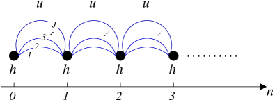
Refer to caption
Figure 3: Chain structure used in the decimation method.

The method works as follows. Suppose we want to solve (EH)G(E)=I𝐸𝐻𝐺𝐸𝐼(E-H)\,G(E)=I for the operator G(E)𝐺𝐸G(E), where the Hamiltonian operator H𝐻H is defined over a chain where each site has an arbitrary basis of dimension J𝐽J but only nearest-neighbor inter-site connections exist (see Fig. 3). We assume that all these connections are represented by operators u𝑢u (left-to-right) and usuperscript𝑢u^{\dagger} (right-to-left). The local Hamiltonian is identical for all sites and denoted by hh. Since, by definition, the Green’s function obeys

[(EH)G(E)]n,m=δn,m,subscriptdelimited-[]𝐸𝐻𝐺𝐸𝑛𝑚subscript𝛿𝑛𝑚\left[(E-H)\,G(E)\right]_{n,m}=\delta_{n,m}, (68)

it follows that

(Eh)G0,0𝐸subscript𝐺00\displaystyle(E-h)\,G_{0,0} =\displaystyle= I+uG1,0,𝐼𝑢subscript𝐺10\displaystyle I+u\,G_{1,0}, (69)
(Eh)G1,0𝐸subscript𝐺10\displaystyle(E-h)\,G_{1,0} =\displaystyle= uG2,0+uG0,0,𝑢subscript𝐺20superscript𝑢subscript𝐺00\displaystyle u\,G_{2,0}+u^{\dagger}G_{0,0},
\displaystyle\vdots
(Eh)Gn,0𝐸subscript𝐺𝑛0\displaystyle(E-h)\,G_{n,0} =\displaystyle= uGn+1,0+uGn1,0,𝑢subscript𝐺𝑛10superscript𝑢subscript𝐺𝑛10\displaystyle u\,G_{n+1,0}+u^{\dagger}G_{n-1,0}, (71)

with n1𝑛1n\geq 1. Using Eq. (4.3), we find that

G1,0=(Eh)1(uG2,0+uG0,0),subscript𝐺10superscript𝐸1𝑢subscript𝐺20superscript𝑢subscript𝐺00G_{1,0}=(E-h)^{-1}\left(u\,G_{2,0}+u^{\dagger}G_{0,0}\right), (72)

which can be combined with Eq. (69) to yield

(Eh)G0,0=I+u(Eh)1(uG2,0+uG0,0),𝐸subscript𝐺00𝐼𝑢superscript𝐸1𝑢subscript𝐺20superscript𝑢subscript𝐺00(E-h)\,G_{0,0}=I+u\,(E-h)^{-1}\left(u\,G_{2,0}+u^{\dagger}G_{0,0}\right), (73)

which can be rewritten as

[Ehu(Eh)1u]G0,0=I+u(Eh)1uG2,0.delimited-[]𝐸𝑢superscript𝐸1superscript𝑢subscript𝐺00𝐼𝑢superscript𝐸1𝑢subscript𝐺20\left[E-h-u\,(E-h)^{-1}u^{\dagger}\right]\,G_{0,0}=I+u\,(E-h)^{-1}u\,G_{2,0}. (74)

Notice that we can relate G2,0subscript𝐺20G_{2,0} to G0,0subscript𝐺00G_{0,0} without involving G1,0subscript𝐺10G_{1,0}.

The same trick can be employed for any value of n𝑛n. From Eq. (71), we can write

Gn+1,0=(Eh)1(uGn+2,0+uGn,0),subscript𝐺𝑛10superscript𝐸1𝑢subscript𝐺𝑛20superscript𝑢subscript𝐺𝑛0G_{n+1,0}=(E-h)^{-1}\left(u\,G_{n+2,0}+u^{\dagger}G_{n,0}\right), (75)

and

Gn1,0=(Eh)1(uGn2,0+uGn,0).subscript𝐺𝑛10superscript𝐸1superscript𝑢subscript𝐺𝑛20𝑢subscript𝐺𝑛0G_{n-1,0}=(E-h)^{-1}\left(u^{\dagger}G_{n-2,0}+u\,G_{n,0}\right). (76)

These equations can be combined with Eq. (71) to yield

(Eh)Gn,0=𝐸subscript𝐺𝑛0absent\displaystyle(E-h)\,G_{n,0}= u(Eh)1(uGn+2,0+uGn,0)+limit-from𝑢superscript𝐸1𝑢subscript𝐺𝑛20superscript𝑢subscript𝐺𝑛0\displaystyle\,u\,(E-h)^{-1}\left(u\,G_{n+2,0}+u^{\dagger}G_{n,0}\right)+
u(Eh)1(uGn,0+uGn2,0),superscript𝑢superscript𝐸1𝑢subscript𝐺𝑛0superscript𝑢subscript𝐺𝑛20\displaystyle\,u^{\dagger}(E-h)^{-1}\left(u\,G_{n,0}+u^{\dagger}G_{n-2,0}\right), (77)

which can be rewritten as

[Ehu(Eh)1uu(Eh)1u]Gn,0=delimited-[]𝐸𝑢superscript𝐸1superscript𝑢superscript𝑢superscript𝐸1𝑢subscript𝐺𝑛0absent\displaystyle\left[E-h-u\,(E-h)^{-1}u^{\dagger}-u^{\dagger}(E-h)^{-1}u\right]\,G_{n,0}=
u(Eh)1uGn+2,0+u(Eh)1uGn2,0.𝑢superscript𝐸1𝑢subscript𝐺𝑛20superscript𝑢superscript𝐸1superscript𝑢subscript𝐺𝑛20\displaystyle\quad\qquad u\,(E-h)^{-1}u\,G_{n+2,0}+u^{\dagger}(E-h)^{-1}u^{\dagger}G_{n-2,0}. (78)

Equations (74) and (4.3) generate a new recursion series involving only even sites:

(Eε1s)G0,0𝐸superscriptsubscript𝜀1𝑠subscript𝐺00\displaystyle(E-\varepsilon_{1}^{s})\,G_{0,0} =\displaystyle= I+α1G2,0𝐼subscript𝛼1subscript𝐺20\displaystyle I+\alpha_{1}\,G_{2,0} (79)
(Eε1)G2,0𝐸subscript𝜀1subscript𝐺20\displaystyle(E-\varepsilon_{1})\,G_{2,0} =\displaystyle= α1G4,0+β1G0,0subscript𝛼1subscript𝐺40subscript𝛽1subscript𝐺00\displaystyle\alpha_{1}\,G_{4,0}+\beta_{1}\,G_{0,0}
\displaystyle\vdots
(Eε1)Gn,0𝐸subscript𝜀1subscript𝐺𝑛0\displaystyle(E-\varepsilon_{1})\,G_{n,0} =\displaystyle= α1Gn+2,0+β1Gn2,0subscript𝛼1subscript𝐺𝑛20subscript𝛽1subscript𝐺𝑛20\displaystyle\alpha_{1}\,G_{n+2,0}+\beta_{1}\,G_{n-2,0} (81)

with

α1subscript𝛼1\displaystyle\alpha_{1} =\displaystyle= u(Eh)1u𝑢superscript𝐸1𝑢\displaystyle u\,(E-h)^{-1}u (82)
β1subscript𝛽1\displaystyle\beta_{1} =\displaystyle= u(Eh)1usuperscript𝑢superscript𝐸1superscript𝑢\displaystyle u^{\dagger}(E-h)^{-1}u^{\dagger} (83)
ε1ssuperscriptsubscript𝜀1𝑠\displaystyle\varepsilon_{1}^{s} =\displaystyle= h+u(Eh)1u𝑢superscript𝐸1superscript𝑢\displaystyle h+u\,(E-h)^{-1}u^{\dagger} (84)
ε1subscript𝜀1\displaystyle\varepsilon_{1} =\displaystyle= ε1s+u(Eh)1u.superscriptsubscript𝜀1𝑠superscript𝑢superscript𝐸1𝑢\displaystyle\varepsilon_{1}^{s}+u^{\dagger}(E-h)^{-1}u. (85)

Even though Eqs. (79) to (81) involve only even sites (i.e., multiples of 21superscript212^{1}), they are identical in form to Eqs. (4.3) and (71). Therefore, we can repeat this procedure k𝑘k times until the recursion relations involve only sites that are multiple of 2ksuperscript2𝑘2^{k}, namely,

(Eεks)G0,0𝐸superscriptsubscript𝜀𝑘𝑠subscript𝐺00\displaystyle(E-\varepsilon_{k}^{s})\,G_{0,0} =\displaystyle= I+αkG2,0𝐼subscript𝛼𝑘subscript𝐺20\displaystyle I+\alpha_{k}\,G_{2,0} (86)
(Eεk)G2k,0𝐸subscript𝜀𝑘subscript𝐺superscript2𝑘0\displaystyle(E-\varepsilon_{k})\,G_{2^{k},0} =\displaystyle= αkG2k2,0+βkG0,0subscript𝛼𝑘subscript𝐺superscript2𝑘20subscript𝛽𝑘subscript𝐺00\displaystyle\alpha_{k}\,G_{2^{k}\cdot 2,0}+\beta_{k}\,G_{0,0}
\displaystyle\vdots
(Eεk)G2kn,0𝐸subscript𝜀𝑘subscript𝐺superscript2𝑘𝑛0\displaystyle(E-\varepsilon_{k})\,G_{2^{k}\cdot n,0} =\displaystyle= αkG2k(n+1),0+βkG2k(n1),0subscript𝛼𝑘subscript𝐺superscript2𝑘𝑛10subscript𝛽𝑘subscript𝐺superscript2𝑘𝑛10\displaystyle\alpha_{k}\,G_{2^{k}\cdot(n+1),0}+\beta_{k}\,G_{2^{k}\cdot(n-1),0} (88)

with n1𝑛1n\geq 1 and

αksubscript𝛼𝑘\displaystyle\alpha_{k} =\displaystyle= αk1(Eεk1)1αk1,subscript𝛼𝑘1superscript𝐸subscript𝜀𝑘11subscript𝛼𝑘1\displaystyle\alpha_{k-1}\,(E-\varepsilon_{k-1})^{-1}\alpha_{k-1}, (89)
βksubscript𝛽𝑘\displaystyle\beta_{k} =\displaystyle= βk1(Eεk1)1βk1,subscript𝛽𝑘1superscript𝐸subscript𝜀𝑘11subscript𝛽𝑘1\displaystyle\beta_{k-1}\,(E-\varepsilon_{k-1})^{-1}\beta_{k-1}, (90)
εkssuperscriptsubscript𝜀𝑘𝑠\displaystyle\varepsilon_{k}^{s} =\displaystyle= εk1+αk1(Eεk1)1βk1,subscript𝜀𝑘1subscript𝛼𝑘1superscript𝐸subscript𝜀𝑘11subscript𝛽𝑘1\displaystyle\varepsilon_{k-1}+\alpha_{k-1}(E-\varepsilon_{k-1})^{-1}\,\beta_{k-1}, (91)
εksubscript𝜀𝑘\displaystyle\varepsilon_{k} =\displaystyle= εks+βk1(Eεk1)1αk1.superscriptsubscript𝜀𝑘𝑠subscript𝛽𝑘1superscript𝐸subscript𝜀𝑘11subscript𝛼𝑘1\displaystyle\varepsilon_{k}^{s}+\beta_{k-1}(E-\varepsilon_{k-1})^{-1}\alpha_{k-1}. (92)

The decimation can stop when αknormsubscript𝛼𝑘||\alpha_{k}|| and βknormsubscript𝛽𝑘||\beta_{k}|| are sufficiently small, in which case we can approximate

G0,0(Eεks)1.subscript𝐺00superscript𝐸superscriptsubscript𝜀𝑘𝑠1G_{0,0}\approx(E-\varepsilon_{k}^{s})^{-1}. (93)

This provides the Green’s function for the “surface” slice, which can then be related to the lead Green’s functions G0Lsubscriptsuperscript𝐺𝐿0G^{L}_{0} and GN+1Rsuperscriptsubscript𝐺𝑁1𝑅G_{N+1}^{R}.

Note that one needs to add a small positive imaginary part to E𝐸E, namely, EE+iη𝐸𝐸𝑖𝜂E\rightarrow E+i\eta, in order to generate retarded Green’s functions. On the practical side, an increase of η𝜂\eta helps to speed up the convergence but spoils the accuracy of G0,0rsubscriptsuperscript𝐺𝑟00G^{r}_{0,0} at the order of η/t𝜂𝑡\eta/t. Provided that η/t1much-less-than𝜂𝑡1\eta/t\ll 1, adding an imaginary part to E𝐸E has little effect on the computation of graphene transport properties for |E|/η1much-greater-than𝐸𝜂1|E|/\eta\gg 1, except for a small energy interval around the charge neutrality point, where E=0𝐸0E=0.

4.3.1 Square lattice lead

Refer to caption
Figure 4: Structure of the square lattice lead. The slice with n=0𝑛0n=0 corresponds to the “surface” which will be attached to the system. Slices for decimation are denoted by the boxes with dashed lines.

From Fig. 4, we see that each decimation site corresponds to a regular open vertical chain with J𝐽J lattice sites. Therefore,

h(j,j)=μ=1Jϕμ(j)ϕμ(j)Eμ,𝑗superscript𝑗superscriptsubscript𝜇1𝐽subscriptitalic-ϕ𝜇𝑗subscriptitalic-ϕ𝜇superscript𝑗subscript𝐸𝜇h(j,j^{\prime})=\sum_{\mu=1}^{J}\phi_{\mu}(j)\,\phi_{\mu}(j^{\prime})\,E_{\mu}, (94)

and

u(j,j)=tδj,j.𝑢𝑗superscript𝑗𝑡subscript𝛿𝑗superscript𝑗u(j,j^{\prime})=-t\,\delta_{j,j^{\prime}}. (95)

where t𝑡t is the nearest-neighbor hopping amplitude, j,j=1,,Jformulae-sequence𝑗superscript𝑗1𝐽j,j^{\prime}=1,\ldots,J, μ=1,,J𝜇1𝐽\mu=1,\ldots,J,

ϕμ(j)=subscriptitalic-ϕ𝜇𝑗absent\displaystyle\phi_{\mu}(j)= 2J+1sin(πμjJ+1),and2𝐽1𝜋𝜇𝑗𝐽1and\displaystyle\,\sqrt{\frac{2}{J+1}}\,\sin\left(\frac{\pi\mu j}{J+1}\right),\quad{\rm and}\quad
Eμ=subscript𝐸𝜇absent\displaystyle E_{\mu}= 2tcos(πμJ+1).2𝑡𝜋𝜇𝐽1\displaystyle\,-2t\,\cos\left(\frac{\pi\mu}{J+1}\right). (96)

From Eqs. (94) and (95), we derive the relations

α1(j,j)=t2[(Eh)1]j,j,subscript𝛼1𝑗superscript𝑗superscript𝑡2subscriptdelimited-[]superscript𝐸1𝑗superscript𝑗\alpha_{1}(j,j^{\prime})=t^{2}\,\left[(E-h)^{-1}\right]_{j,j^{\prime}}, (97)
ε1s(j,j)=h(j,j)+α1(j,j),superscriptsubscript𝜀1𝑠𝑗superscript𝑗𝑗superscript𝑗subscript𝛼1𝑗superscript𝑗\varepsilon_{1}^{s}(j,j^{\prime})=h(j,j^{\prime})+\alpha_{1}(j,j^{\prime}), (98)

and

ε1s(j,j)=h(j,j)+2α1(j,j).superscriptsubscript𝜀1𝑠𝑗superscript𝑗𝑗superscript𝑗2subscript𝛼1𝑗superscript𝑗\varepsilon_{1}^{s}(j,j^{\prime})=h(j,j^{\prime})+2\alpha_{1}(j,j^{\prime}). (99)

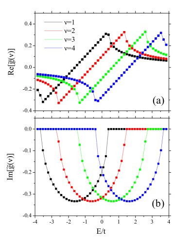
Figure 5 shows a comparison between the analytical and decimation results for the Gr(E)superscript𝐺𝑟𝐸G^{r}(E) of a square lattice of width J=M=6𝐽𝑀6J=M=6, projected onto the eigenchannel basis. Notice the excellent agreement.
Refer to caption
Figure 5: Real (a) and imaginary part (b) of the Green function of a semi-infinite square lattice in the channel (diagonal) representation, g~(μ)~𝑔𝜇\widetilde{g}(\mu), as a function of energy. J=4𝐽4J=4. The solid lines represent the exact analytic result, whereas the squares were numerically obtained through the decimation method for η=106𝜂superscript106\eta=10^{-6} and k=10𝑘10k=10.

4.3.2 Honeycomb lattice lead – armchair edges

Refer to caption
Figure 6: (a) Structure of the honeycomb armchair lead. Note that the number of interconnect channels runs from 1 to J𝐽J, while the number of vertical coordinate points in the slice is M=2J+1𝑀2𝐽1M=2J+1. The slices for decimation are defined by the boxed regions. (b) Internal index structure of the elementary slice.

For the honeycomb lattice with armchair edges, the elementary slice contains J𝐽J stacked hexagons. Thus, M=2J+1𝑀2𝐽1M=2J+1, where M𝑀M is the vertical number of atoms. The slice has the structure of a vertical ladder chain (2M2𝑀2M atoms). In this case there is no simple formula for the eigenstates of hh. The matrix hh, which is 2M×2M2𝑀2𝑀2M\times 2M dimensional, reads

h~=(tttttttttttttttttttt).~missing-subexpression𝑡𝑡missing-subexpressionmissing-subexpressionmissing-subexpressionmissing-subexpressionmissing-subexpressionmissing-subexpression𝑡missing-subexpressionmissing-subexpression𝑡missing-subexpressionmissing-subexpressionmissing-subexpressionmissing-subexpressionmissing-subexpression𝑡missing-subexpressionmissing-subexpression𝑡𝑡missing-subexpressionmissing-subexpressionmissing-subexpressionmissing-subexpressionmissing-subexpression𝑡𝑡missing-subexpressionmissing-subexpression𝑡missing-subexpressionmissing-subexpressionmissing-subexpressionmissing-subexpressionmissing-subexpression𝑡missing-subexpressionmissing-subexpression𝑡𝑡missing-subexpressionmissing-subexpressionmissing-subexpressionmissing-subexpressionmissing-subexpression𝑡𝑡missing-subexpressionmissing-subexpression𝑡missing-subexpressionmissing-subexpressionmissing-subexpressionmissing-subexpressionmissing-subexpression𝑡missing-subexpressionmissing-subexpression𝑡missing-subexpressionmissing-subexpressionmissing-subexpressionmissing-subexpressionmissing-subexpressionmissing-subexpression𝑡𝑡missing-subexpressionmissing-subexpressionmissing-subexpressionmissing-subexpressionmissing-subexpressionmissing-subexpressionmissing-subexpressionmissing-subexpressionmissing-subexpressionmissing-subexpression\tilde{h}=\left(\begin{array}[]{ccccccccc}&-t&-t&&&&&&\\ -t&&&-t&&&&&\\ -t&&&-t&-t&&&&\\ &-t&-t&&&-t&&&\\ &&-t&&&-t&-t&&\\ &&&-t&-t&&&-t&\\ &&&&-t&&&-t&\\ &&&&&-t&-t&&\\ &&&&&&&&\ddots\end{array}\right). (100)

Let us call {ϕμ(m)}subscriptitalic-ϕ𝜇𝑚\{\phi_{\mu}(m)\} its eigenvectors and {Eμ}subscript𝐸𝜇\{E_{\mu}\} its eigenvalues, with μ=1,,2M𝜇12𝑀\mu=1,\ldots,2M. Then,

h(j,j)=μ=12Mϕμ(4j)ϕμ(4j1)Eμ,𝑗superscript𝑗superscriptsubscript𝜇12𝑀subscriptitalic-ϕ𝜇4𝑗subscriptitalic-ϕ𝜇4superscript𝑗1subscript𝐸𝜇h(j,j^{\prime})=\sum_{\mu=1}^{2M}\phi_{\mu}(4j)\,\phi_{\mu}(4j^{\prime}-1)\,E_{\mu}, (101)

with j,j=1,,Jformulae-sequence𝑗superscript𝑗1𝐽j,j^{\prime}=1,\ldots,J. Everything else is similar to Sec. 4.3.1.

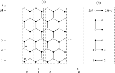
4.3.3 Honeycomb lattice lead – zigzag edges
Refer to caption
Figure 7: (a) Structure of the honeycomb zigzag lead. Note that the number of interconnect channels runs from 1 to J=M𝐽𝑀J=M, where M𝑀M is the number of vertical coordinate points in the graphene. The slices for decimation are defined by the boxed regions. (b) Internal index structure of the elementary slice.

For the zigzag graphene lead, there is a direct correspondence between slice channels and the vertical indices of atomic positions: M=J𝑀𝐽M=J. The elementary slice is a open vertical chain of length 2M2𝑀2M. Its eigenfunctions and eigenvalues are

ϕμ(l)=22M+1sin(πμl2M+1),andsubscriptitalic-ϕ𝜇𝑙22𝑀1𝜋𝜇𝑙2𝑀1and\displaystyle\phi_{\mu}(l)=\sqrt{\frac{2}{2M+1}}\,\sin\left(\frac{\pi\mu l}{2M+1}\right),\quad{\rm and}
Eμ=2tcos(πμ2M+1),subscript𝐸𝜇2𝑡𝜋𝜇2𝑀1\displaystyle E_{\mu}=-2t\,\cos\left(\frac{\pi\mu}{2M+1}\right), (102)

with l=1,,M𝑙1𝑀l=1,\ldots,M and μ=1,,2M𝜇12𝑀\mu=1,\ldots,2M. The slice matrix reads

h(j,j)=μ=12Mϕμ(2j1)ϕμ(2j)Eμ,𝑗superscript𝑗superscriptsubscript𝜇12𝑀subscriptitalic-ϕ𝜇2𝑗1subscriptitalic-ϕ𝜇2superscript𝑗subscript𝐸𝜇h(j,j^{\prime})=\sum_{\mu=1}^{2M}\phi_{\mu}(2j-1)\,\phi_{\mu}(2j^{\prime})\,E_{\mu}, (103)

with j,j=1,,Mformulae-sequence𝑗superscript𝑗1𝑀j,j^{\prime}=1,\ldots,M. All other aspects are identical to Sec. 4.3.1.

5 Device Green’s Function

The device Green’s function Gi,jsubscript𝐺𝑖𝑗G_{i,j} can be used to describe nearly all the physics of transport and its calculation is where most of the computational time is spent. This is where any optimization of the computational method is most welcome, particularly in the study of disorder effects in the electronic transport when extensive disorder averaging is required. With the RGF method one can compute Gi,jsubscript𝐺𝑖𝑗G_{i,j} for a large variety of settings. For instance, the graphene sheet can have an arbitrary number of layers and different edge orientations, namely, zigzag, armchair, and chiral. Also, the tight-binding model can include next-nearest neighbor hopping terms in addition to the nearest neighbor ones. These elements have to be taken into account when choosing the slice unit cell employed by the recursive method. The description of disorder modeling is postponed to section 8.

In this Section we present efficient slicing schemes for graphene monolayers with armchair and zigzag edges.

5.1 Slicing armchair lattices

For rectangular geometries, the bottleneck of the recursive method is the matrix inversion required for adding a new slice [see Eq. (32)]. Thus, it is always important to try to minimize the number of sites in the slice. Having this in mind, there is a way to mount the armchair slices which reduces the number of sites per slice without introducing next-to-nearest neighbor hopping. It is based on the lattice deformation shown in Fig. 8.

Refer to caption
Figure 8: Efficient way to slice an armchair graphene ribbon (the so-called “pine tree” configuration). Atoms from different sublattices are indicated by empty (A) and full (B) circles. a0subscript𝑎0a_{0} is the lattice constant. The dashed lines indicate vertical slices.

The relations between lattice size and graphene sheet dimensions for the efficient armchair slicing are

La0=32(N21)+36andWa0=M1.formulae-sequence𝐿subscript𝑎032𝑁2136and𝑊subscript𝑎0𝑀1\frac{L}{a_{0}}=\frac{\sqrt{3}}{2}\left(\frac{N}{2}-1\right)+\frac{\sqrt{3}}{6}\quad{\rm and}\quad\frac{W}{a_{0}}=M-1. (104)

5.2 Slicing zigzag lattices

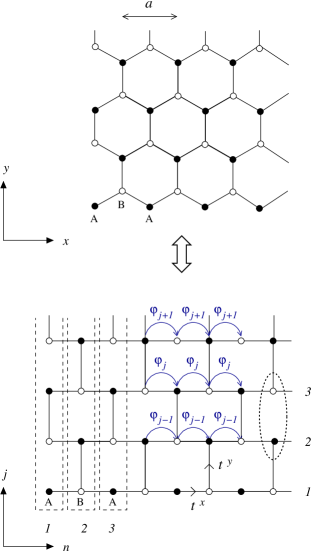
The zigzag geometry is shown in Fig. 9. The real structure is shown on the left-hand side (honeycomb lattice). An equivalent square lattice with missing vertical bonds is also shown (the so-called “brick wall” configuration). For zigzag edge ribbons there is no efficient, alternative slicing that minimizes the number of sites per slice without creating a next-to-nearest neighbor connectivity.
Refer to caption
Figure 9: Graphene strip with zigzag edges. Atoms from different sublattices are indicated by empty (A) and full (B) circles. a0subscript𝑎0a_{0} is the lattice constant. The dashed lines indicate vertical slices and the dotted highlights a dimer. By convention, we set as (1,1) the coordinates of an atom of type A placed at the left bottom corner. The Peierls phases (see appendix B) of the “horizontal” hopping matrix elements are indicated.

By convention, we assume that the site at the left bottom corner of the lattice is of type A. In that way, slices with even and odd number of sites will alternate as we move horizontally. Two cases will need to be considered separately: M𝑀M odd and M𝑀M even. However, both cases share a common trend, namely, the presence of dimers and isolated sites (at the bottom and/or at the top of the slice). Therefore, finding the Green’s function of an isolated slice is a very simple exercise.

The relations between lattice size and graphene sheet dimensions for the zigzag slicing are

Wa0=32(M1)+36andLa0=N12.formulae-sequence𝑊subscript𝑎032𝑀136and𝐿subscript𝑎0𝑁12\frac{W}{a_{0}}=\frac{\sqrt{3}}{2}(M-1)+\frac{\sqrt{3}}{6}\quad{\rm and}\quad\frac{L}{a_{0}}=\frac{N-1}{2}. (105)

6 Evaluating Local Quantities

In addition to the transmission 𝒯𝒯{\cal T}, the RGF method can be used to calculate other quantities such as the local density of states (e.g. Metalidis05 ) and the local current density (e.g. Todorov02 ; Cresti03 ).

6.1 Local density of states

The local density of states (LDOS) can be easily evaluated if one knows the exact retarded Green’s function at a given site:

ρ(n,j;E)=1πIm[Gn,nr(j,j;E)].𝜌𝑛𝑗𝐸1𝜋Imdelimited-[]subscriptsuperscript𝐺𝑟𝑛𝑛𝑗𝑗𝐸\rho(n,j;E)=-\frac{1}{\pi}\,{\rm Im}\left[G^{r}_{n,n}(j,j;E)\right]. (106)

The exact local Green’s function is evaluated using Eq. (3.4). Conductance calculations require just a single sweep through the lattice, since the transmission formula (15) only needs Grsuperscript𝐺𝑟G^{r} evaluated at the slices corresponding to the contacts. In contrast, the LDOS demands the calculation of Grsuperscript𝐺𝑟G^{r} at all lattice slices of interest, which further increases the computational cost linearly with N𝑁N, resulting in O(N2M3)𝑂superscript𝑁2superscript𝑀3O(N^{2}M^{3}). Let us provide an example of a situation where the LDOS plays a central role and needs to be evaluated.

Numerous studies have addressed the possibility of local magnetic moment formation in graphene either due to zigzag terminations at the edges in graphene nanoribbons or due to vacancies in graphene sheets (for a review, see Ref. Yazyev10 ). The effect can be understood through the Stoner mechanism of magnetism, which requires an enhanced LDOS when strong electron-electron interaction as present, as originally proposed in Ref. Son06 using the Density Functional Theory (DFT). The tight-binding Hamiltonian, Eq. (4), can be modified to reproduce the DFT results by adding a Hubbard mean-field term Son06 , namely,

H=i<j,σ𝐻subscript𝑖𝑗𝜎\displaystyle H=-\sum_{i<j,\sigma} (tijci,σcj,σ+H.c.)\displaystyle\left(t_{ij}c^{\dagger}_{i,\sigma}c_{j,\sigma}+{\rm H.c.}\right)
+i,σ(Vi+Uni,σ)ci,σci,σ,subscript𝑖𝜎subscript𝑉𝑖𝑈delimited-⟨⟩subscript𝑛𝑖𝜎subscriptsuperscript𝑐𝑖𝜎subscript𝑐𝑖𝜎\displaystyle+\,\sum_{i,\sigma}\Big{(}V_{i}+U\langle n_{i,-\sigma}\rangle\Big{)}c^{\dagger}_{i,\sigma}c_{i,\sigma}, (107)

where the operators ci,σsubscriptsuperscript𝑐𝑖𝜎c^{\dagger}_{i,\sigma} and ci,σsubscript𝑐𝑖𝜎c_{i,\sigma} create and annihilate an electron of spin projection σ𝜎\sigma at at the site i𝑖i. As standard, ni,σdelimited-⟨⟩subscript𝑛𝑖𝜎\langle n_{i,\sigma}\rangle is the occupation number and U𝑈U is the on-site electron-electron interaction strength. In graphene, U𝑈U is usually fitted to reproduce the DFT band structure calculations for translation invariant systems (for which Visubscript𝑉𝑖V_{i} is constant). As we discuss in Sec. 8, by a suitable choice of the parameters Visubscript𝑉𝑖V_{i} and tijsubscript𝑡𝑖𝑗t_{ij}, the Hamiltonian (6.1) becomes an excellent framework to model disorder as well.

In general, the occupation numbers ni,σdelimited-⟨⟩subscript𝑛𝑖𝜎\langle n_{i,\sigma}\rangle that appear in Eq. (6.1) can be obtained from nonequilibrium Green’s functions HaugJauho08 . In the linear response regime, a simplification allows one to express ni,σdelimited-⟨⟩subscript𝑛𝑖𝜎\langle n_{i,\sigma}\rangle in terms of an equilibrium Green’s function, namely,

ni,σ=1π𝑑EIm[Gn,n;σr(j,j;E)]f(Eμ).delimited-⟨⟩subscript𝑛𝑖𝜎1𝜋superscriptsubscriptdifferential-d𝐸Imdelimited-[]subscriptsuperscript𝐺𝑟𝑛𝑛𝜎𝑗𝑗𝐸𝑓𝐸𝜇\langle n_{i,\sigma}\rangle=-\frac{1}{\pi}\int_{-\infty}^{\infty}dE\,\mbox{Im}\,[G^{r}_{n,n;\sigma}(j,j;E)]f(E-\mu). (108)

where i(j,n)𝑖𝑗𝑛i\equiv(j,n). Note that Eqs. (6.1) and (108) have to be solved self-consistently.

The large number of poles of Gr(E)superscript𝐺𝑟𝐸G^{r}(E) makes impractical the integration of the r.h.s. of Eq. (108) on the real axis, a difficulty shared with transport studies on molecular electronics, see e.g. Ref. Xue01 . An optimized strategy to implement an efficient integration along a complex plane contour is presented in Refs. Areshkin09 ; Areshkin10 .

Another frequent application of LDOS occurs in the evaluation of the local charge density. The latter can be calculated from the LDOS through the expression

nc(n,j;EF)=1Aμ(n,j)EF𝑑Eρ(n,j;E),subscript𝑛𝑐𝑛𝑗subscript𝐸𝐹1𝐴superscriptsubscript𝜇𝑛𝑗subscript𝐸𝐹differential-d𝐸𝜌𝑛𝑗𝐸n_{c}(n,j;E_{F})=\frac{1}{A}\,\int_{\mu(n,j)}^{E_{F}}dE\,\rho(n,j;E), (109)

where A𝐴A is the sheet area and μ(n,j)𝜇𝑛𝑗\mu(n,j) denotes the local chemical potential. Note that in n𝑛n-type regions, EF>μsubscript𝐸𝐹𝜇E_{F}>\mu and therefore the integral is over positive energies (“electrons”), while in p𝑝p-type regions, EF<μsubscript𝐸𝐹𝜇E_{F}<\mu and the integral is over negative energies (“holes”). The local chemical potential is evaluated with respect to EF=0subscript𝐸𝐹0E_{F}=0,

μ(n,j)=V(n,j),𝜇𝑛𝑗𝑉𝑛𝑗\mu(n,j)=V(n,j), (110)

where the background potential V(n,j)𝑉𝑛𝑗V(n,j) includes the gate voltage.

6.2 Local current density

The local current density is involves more complex calculation than the LDOS. Several methods were developed in the literature (see e.g. Ref. Todorov02 ). The bond current between two neighboring sites of lattice coordinates (n,j)𝑛𝑗(n,j) and (n,j)superscript𝑛superscript𝑗(n^{\prime},j^{\prime}) is obtained using the equations-of-motion method for nonequilibrium Green’s functions (see e.g. HaugJauho08 ) and reads Caroli71

I(n,j)(n,j)=2eh𝑑Esubscript𝐼𝑛𝑗superscript𝑛superscript𝑗2𝑒differential-d𝐸\displaystyle I_{(n,j)\rightarrow(n^{\prime},j^{\prime})}=-\frac{2e}{h}\int dE [Un,n(j,j)Gn,n<(j,j)\displaystyle\left[\,U_{n,n^{\prime}}(j,j^{\prime})G^{<}_{n^{\prime},n}(j^{\prime},j)\right.
Un,n(j,j)Gn,n<(j,j)],\displaystyle\left.\;\;\;\;-U_{n^{\prime},n}(j^{\prime},j)G^{<}_{n,n^{\prime}}(j,j^{\prime})\right], (111)

where G<superscript𝐺G^{<} is the lesser Green’s function of the system. 222There are several good textbooks, such as Refs. HaugJauho08 ; BruusFlensberg04 ; NazarovBlanter09 , that discuss nonequilibrium Green’s functions. In particular, Ref. HaugJauho08 concisely covers all required background material. We refer the reader to these books for the derivation of expressions involving G<superscript𝐺G^{<} and related functions and further insight into the subject. For the tight-binding model with nearest-neighbor hopping, there are two situations to consider. First, n=n𝑛superscript𝑛n=n^{\prime}, in which case j=j±1superscript𝑗plus-or-minus𝑗1j^{\prime}=j\pm 1 and the current is intra-slice. Second, when n=n±1superscript𝑛plus-or-minus𝑛1n^{\prime}=n\pm 1, the current is inter-slice and j=jsuperscript𝑗𝑗j^{\prime}=j or j=j±1superscript𝑗plus-or-minus𝑗1j^{\prime}=j\pm 1, at most. Notice that in the absence of magnetic fields, time-reversal symmetry requires Un,n(j,j)=Un,n(j,j)subscript𝑈𝑛superscript𝑛𝑗superscript𝑗subscript𝑈superscript𝑛𝑛superscript𝑗𝑗U_{n,n^{\prime}}(j,j^{\prime})=U_{n^{\prime},n}(j^{\prime},j). In addition, in equilibrium conditions, the lesser Green’s function is a symmetric matrix, leading to a zero bond current, as expected. Thus, local currents can only appear through the application of a magnetic field (which breaks time-reversal symmetry) or when a finite bias voltage between contacts exists.

Equation (111) requires the calculation of the exact lesser Green’s function for sites in the bulk of the system. This can be done recursively, starting from the equilibrium Green’s function of the leads (see Sec. 6.3). An alternative approach, suitable for transport in the linear regime, is to use the elimination technique developed in Ref. Cresti03 , where only retarded and advanced Green’s functions are required and the energy integration is avoided. The computational cost is this approach also scales as O(N2M3)𝑂superscript𝑁2superscript𝑀3O(N^{2}M^{3}).

For plotting current fields, it is useful to define the local, on-site, outgoing vector current as

In,j=n,ja(n,j)(n,j)I(n,j)(n,j),subscript𝐼𝑛𝑗subscriptsuperscript𝑛superscript𝑗subscript𝑎𝑛𝑗superscript𝑛superscript𝑗subscript𝐼𝑛𝑗superscript𝑛superscript𝑗\vec{I}_{n,j}=\sum_{n^{\prime},j^{\prime}}\vec{a}_{(n,j)\rightarrow(n^{\prime},j^{\prime})}\,I_{(n,j)\rightarrow(n^{\prime},j^{\prime})}, (112)

where the sum is over sites (n,j)superscript𝑛superscript𝑗(n^{\prime},j^{\prime}) that are nearest neighbors to site (n,j)𝑛𝑗(n,j) and ak,ksubscript𝑎𝑘superscript𝑘\vec{a}_{k,k^{\prime}} is the lattice vector between sites k𝑘k and ksuperscript𝑘k^{\prime}. Notice that this local vector current does not necessarily fall along any of the bonds coming out of the site (n,j)𝑛𝑗(n,j).

6.3 Recursion for non-equilibrium Green’s functions

In order to evaluate the local current distribution (111) in the most general case, one needs to determine the exact lesser Green’s function, G<superscript𝐺G^{<}. The procedure is the following.

  1. 1.

    We start with the retarded Green’s functions of the leads (which are assumed to be in equilibrium) and use the fluctuation-dissipation relations

    gL<=ifL(gLrgLa),subscriptsuperscript𝑔𝐿𝑖subscript𝑓𝐿superscriptsubscript𝑔𝐿𝑟superscriptsubscript𝑔𝐿𝑎\displaystyle g^{<}_{L}=-if_{L}\left(g_{L}^{r}-g_{L}^{a}\right),\quad (113)
    and
    gR<=ifR(gRrgRa),subscriptsuperscript𝑔𝑅𝑖subscript𝑓𝑅superscriptsubscript𝑔𝑅𝑟superscriptsubscript𝑔𝑅𝑎\displaystyle g^{<}_{R}=-if_{R}\left(g_{R}^{r}-g_{R}^{a}\right), (114)

    where the advanced Green’s functions obey gLa=(gLr)superscriptsubscript𝑔𝐿𝑎superscriptsuperscriptsubscript𝑔𝐿𝑟g_{L}^{a}=\left(g_{L}^{r}\right)^{\dagger} and gRa=(gRr)superscriptsubscript𝑔𝑅𝑎superscriptsuperscriptsubscript𝑔𝑅𝑟g_{R}^{a}=\left(g_{R}^{r}\right)^{\dagger}. Here, fLsubscript𝑓𝐿f_{L} and fRsubscript𝑓𝑅f_{R} denote the Fermi distributions in the left and right leads, respectively.

  2. 2.

    For the left-to-right sweep, we first determine the retarded Green’s function at the n𝑛nth slice and then obtain the lesser Green’s function using the expression

    Gn,nL,<=Gn,nL,rΣn,nL,<Gn,nL,a,subscriptsuperscript𝐺𝐿𝑛𝑛subscriptsuperscript𝐺𝐿𝑟𝑛𝑛subscriptsuperscriptΣ𝐿𝑛𝑛subscriptsuperscript𝐺𝐿𝑎𝑛𝑛G^{L,<}_{n,n}=G^{L,r}_{n,n}\,\Sigma^{L,<}_{n,n}\,G^{L,a}_{n,n}, (115)

    where the self energy due to the coupling of the n𝑛nth slice to all other slices to the left is given by

    Σn,nL,<=Un,n1Gn1,n1L,<Un1,n.subscriptsuperscriptΣ𝐿𝑛𝑛subscript𝑈𝑛𝑛1subscriptsuperscript𝐺𝐿𝑛1𝑛1subscript𝑈𝑛1𝑛\Sigma^{L,<}_{n,n}=U_{n,n-1}\,G^{L,<}_{n-1,n-1}\,U_{n-1,n}. (116)

    Notice that Gn,nL,a=(Gn,nL,r)subscriptsuperscript𝐺𝐿𝑎𝑛𝑛superscriptsubscriptsuperscript𝐺𝐿𝑟𝑛𝑛G^{L,a}_{n,n}=\left(G^{L,r}_{n,n}\right)^{\dagger} and Un,n1=(Un1,n)subscript𝑈𝑛𝑛1superscriptsubscript𝑈𝑛1𝑛U_{n,n-1}=\left(U_{n-1,n}\right)^{\dagger}. Thus, we obtain the recurrence relation

    Gn,nL,<=(Gn,nL,rUn,n1)Gn1,n1L,<(Gn,nL,rUn,n1).superscriptsubscript𝐺𝑛𝑛𝐿superscriptsubscript𝐺𝑛𝑛𝐿𝑟subscript𝑈𝑛𝑛1superscriptsubscript𝐺𝑛1𝑛1𝐿superscriptsuperscriptsubscript𝐺𝑛𝑛𝐿𝑟subscript𝑈𝑛𝑛1G_{n,n}^{L,<}=\left(G_{n,n}^{L,r}\,U_{n,n-1}\right)\,G_{n-1,n-1}^{L,<}\,\left(G_{n,n}^{L,r}\,U_{n,n-1}\right)^{\dagger}. (117)
  3. 3.

    For the right-to-left sweep, we apply instead the analogous expression

    Gn,nR,<=Gn,nR,rΣn,nR,<Gn,nR,a,subscriptsuperscript𝐺𝑅𝑛𝑛subscriptsuperscript𝐺𝑅𝑟𝑛𝑛subscriptsuperscriptΣ𝑅𝑛𝑛subscriptsuperscript𝐺𝑅𝑎𝑛𝑛G^{R,<}_{n,n}=G^{R,r}_{n,n}\,\Sigma^{R,<}_{n,n}\,G^{R,a}_{n,n}, (118)

    where

    Σn,nR,<=Un,n+1Gn+1,n+1R,<Un+1,n.subscriptsuperscriptΣ𝑅𝑛𝑛subscript𝑈𝑛𝑛1subscriptsuperscript𝐺𝑅𝑛1𝑛1subscript𝑈𝑛1𝑛\Sigma^{R,<}_{n,n}=U_{n,n+1}\,G^{R,<}_{n+1,n+1}\,U_{n+1,n}. (119)

    Thus, we obtain the other recurrence relation

    Gn,nR,<=(Gn,nR,rUn,n+1)Gn+1,n+1R,<(Gn,nR,rUn,n+1).superscriptsubscript𝐺𝑛𝑛𝑅superscriptsubscript𝐺𝑛𝑛𝑅𝑟subscript𝑈𝑛𝑛1superscriptsubscript𝐺𝑛1𝑛1𝑅superscriptsuperscriptsubscript𝐺𝑛𝑛𝑅𝑟subscript𝑈𝑛𝑛1G_{n,n}^{R,<}=\left(G_{n,n}^{R,r}\,U_{n,n+1}\right)\,G_{n+1,n+1}^{R,<}\,\left(G_{n,n}^{R,r}\,U_{n,n+1}\right)^{\dagger}. (120)
  4. 4.

    In order to join the two sweeps to obtain the exact lesser Green’s function at a given slice, we simply combine left and right self energies and evaluate

    Gn,n<=Gn,nr(Σn,nL,<+Σn,nR,<)Gn,nasubscriptsuperscript𝐺𝑛𝑛subscriptsuperscript𝐺𝑟𝑛𝑛subscriptsuperscriptΣ𝐿𝑛𝑛subscriptsuperscriptΣ𝑅𝑛𝑛subscriptsuperscript𝐺𝑎𝑛𝑛G^{<}_{n,n}=G^{r}_{n,n}\left(\Sigma^{L,<}_{n,n}+\Sigma^{R,<}_{n,n}\right)G^{a}_{n,n} (121)

    using Eqs. (116) and (119) for the self energies.

  5. 5.

    Once the left-to-right and right-to-left Green’s functions are know, the exact inter-slice lesser Green’s functions are obtained using the Dyson-Langreth equations HaugJauho08

    Gn1,n<=Gn1,n1L,rUn1,nGn,n<+Gn1,n1L,<Un1,nGn,na,subscriptsuperscript𝐺𝑛1𝑛subscriptsuperscript𝐺𝐿𝑟𝑛1𝑛1subscript𝑈𝑛1𝑛subscriptsuperscript𝐺𝑛𝑛subscriptsuperscript𝐺𝐿𝑛1𝑛1subscript𝑈𝑛1𝑛subscriptsuperscript𝐺𝑎𝑛𝑛G^{<}_{n-1,n}=G^{L,r}_{n-1,n-1}\,U_{n-1,n}\,G^{<}_{n,n}+G^{L,<}_{n-1,n-1}\,U_{n-1,n}\,G^{a}_{n,n}, (122)
    Gn,n+1<=Gn,nrUn,n+1Gn+1,n+1R,<+Gn,n<Un,n+1Gn+1,n+1R,a,subscriptsuperscript𝐺𝑛𝑛1subscriptsuperscript𝐺𝑟𝑛𝑛subscript𝑈𝑛𝑛1subscriptsuperscript𝐺𝑅𝑛1𝑛1subscriptsuperscript𝐺𝑛𝑛subscript𝑈𝑛𝑛1subscriptsuperscript𝐺𝑅𝑎𝑛1𝑛1G^{<}_{n,n+1}=G^{r}_{n,n}\,U_{n,n+1}\,G^{R,<}_{n+1,n+1}+G^{<}_{n,n}\,U_{n,n+1}\,G^{R,a}_{n+1,n+1}, (123)
    Gn,n1<=Gn,nrUn,n1Gn1,n1L,<+Gn,n<Un,n1Gn1,n1L,a,subscriptsuperscript𝐺𝑛𝑛1subscriptsuperscript𝐺𝑟𝑛𝑛subscript𝑈𝑛𝑛1subscriptsuperscript𝐺𝐿𝑛1𝑛1subscriptsuperscript𝐺𝑛𝑛subscript𝑈𝑛𝑛1subscriptsuperscript𝐺𝐿𝑎𝑛1𝑛1G^{<}_{n,n-1}=G^{r}_{n,n}\,U_{n,n-1}\,G^{L,<}_{n-1,n-1}+G^{<}_{n,n}\,U_{n,n-1}\,G^{L,a}_{n-1,n-1}, (124)

    and

    Gn+1,n<=Gn+1,n+1R,rUn+1,nGn,n<+Gn+1,n+1R,<Un+1,nGn,na.subscriptsuperscript𝐺𝑛1𝑛subscriptsuperscript𝐺𝑅𝑟𝑛1𝑛1subscript𝑈𝑛1𝑛subscriptsuperscript𝐺𝑛𝑛subscriptsuperscript𝐺𝑅𝑛1𝑛1subscript𝑈𝑛1𝑛subscriptsuperscript𝐺𝑎𝑛𝑛G^{<}_{n+1,n}=G^{R,r}_{n+1,n+1}\,U_{n+1,n}\,G^{<}_{n,n}+G^{R,<}_{n+1,n+1}\,U_{n+1,n}\,G^{a}_{n,n}. (125)

6.4 Current conservation

Notice that the current through consecutive slices is conserved. Let us prove that using Eq. 111 and writing

I(n1)n=eh𝑑ETr(Gn,n1<Un1,nUn,n1Gn1,n<)subscript𝐼𝑛1𝑛𝑒differential-d𝐸Trsubscriptsuperscript𝐺𝑛𝑛1subscript𝑈𝑛1𝑛subscript𝑈𝑛𝑛1subscriptsuperscript𝐺𝑛1𝑛I_{(n-1)\rightarrow n}=-\frac{e}{h}\int dE\,{\rm Tr}\left(G^{<}_{n,n-1}\,U_{n-1,n}-U_{n,n-1}\,G^{<}_{n-1,n}\right) (126)

and

In(n+1)=eh𝑑ETr(Gn+1,n<Un,n+1Un+1,nGn,n+1<),subscript𝐼𝑛𝑛1𝑒differential-d𝐸Trsubscriptsuperscript𝐺𝑛1𝑛subscript𝑈𝑛𝑛1subscript𝑈𝑛1𝑛subscriptsuperscript𝐺𝑛𝑛1I_{n\rightarrow(n+1)}=-\frac{e}{h}\int dE\,{\rm Tr}\left(G^{<}_{n+1,n}\,U_{n,n+1}-U_{n+1,n}\,G^{<}_{n,n+1}\right), (127)

where the traces indicate a sum over all sites in the slices n𝑛n and n+1𝑛1n+1, respectively. Since

Gn,n1<Un1,n=Gn,nrΣn,nL,<+Gn,n<Σn,nL,a,subscriptsuperscript𝐺𝑛𝑛1subscript𝑈𝑛1𝑛subscriptsuperscript𝐺𝑟𝑛𝑛superscriptsubscriptΣ𝑛𝑛𝐿subscriptsuperscript𝐺𝑛𝑛subscriptsuperscriptΣ𝐿𝑎𝑛𝑛G^{<}_{n,n-1}\,U_{n-1,n}=G^{r}_{n,n}\,\Sigma_{n,n}^{L,<}+G^{<}_{n,n}\,\Sigma^{L,a}_{n,n}, (128)
Un,n1Gn1,n<=Σn,nL,rGn,n<+Σn,nL,<Gn,na,subscript𝑈𝑛𝑛1subscriptsuperscript𝐺𝑛1𝑛superscriptsubscriptΣ𝑛𝑛𝐿𝑟subscriptsuperscript𝐺𝑛𝑛subscriptsuperscriptΣ𝐿𝑛𝑛subscriptsuperscript𝐺𝑎𝑛𝑛U_{n,n-1}\,G^{<}_{n-1,n}=\Sigma_{n,n}^{L,r}\,G^{<}_{n,n}+\Sigma^{L,<}_{n,n}\,G^{a}_{n,n}, (129)
Gn,n+1<Un+1,n=Gn,nrΣn,nR,<+Gn,n<Σn,nR,a,subscriptsuperscript𝐺𝑛𝑛1subscript𝑈𝑛1𝑛subscriptsuperscript𝐺𝑟𝑛𝑛superscriptsubscriptΣ𝑛𝑛𝑅subscriptsuperscript𝐺𝑛𝑛subscriptsuperscriptΣ𝑅𝑎𝑛𝑛G^{<}_{n,n+1}\,U_{n+1,n}=G^{r}_{n,n}\,\Sigma_{n,n}^{R,<}+G^{<}_{n,n}\,\Sigma^{R,a}_{n,n}, (130)

and

Un,n+1Gn+1,n<=Σn,nR,rGn,n<+Σn,nR,<Gn,na,subscript𝑈𝑛𝑛1subscriptsuperscript𝐺𝑛1𝑛superscriptsubscriptΣ𝑛𝑛𝑅𝑟subscriptsuperscript𝐺𝑛𝑛subscriptsuperscriptΣ𝑅𝑛𝑛subscriptsuperscript𝐺𝑎𝑛𝑛U_{n,n+1}\,G^{<}_{n+1,n}=\Sigma_{n,n}^{R,r}\,G^{<}_{n,n}+\Sigma^{R,<}_{n,n}\,G^{a}_{n,n}, (131)

it is straightforward to show that I(n1)n=In(n+1)subscript𝐼𝑛1𝑛subscript𝐼𝑛𝑛1I_{(n-1)\rightarrow n}=I_{n\rightarrow(n+1)}, which guarantees current conservation. It is also possible to show that the total current leaving any site is zero.

7 Dephasing

The model Hamiltonian (4) describes electrons within the single-particle approximation, disregarding the effects of electron-phonon and electron-electron interactions. Let us call as “environment” all the degrees of freedom that couple to electrons in the real physical device. Even at very low temperatures, due to the interaction with the environment, the quantum interference between different electronic paths typically fades away at lengths larger than the scale φsubscript𝜑\ell_{\varphi}. The latter is called coherence length or dephasing length. Currently, φsubscript𝜑\ell_{\varphi} in graphene experiments can be as high as few microns at low temperatures, decreasing with increasing temperature.

This Section shows how to incorporate dephasing into the RGF method. We follow the phenomenological approach pioneered by Büttiker Buttiker88 and D’Amato and Pastawski DAmato90 and introduce dephasing in the calculations by adding a set of voltage probes to the system. These voltage probes act on selected system sites and have their individual chemical potentials adjusted as not drain or inject any net current. The voltage probes give rise to dephasing because the drained electrons are not phase coherent with the ones injected back. The dephasing length φsubscript𝜑\ell_{\varphi} is related to the number of voltage probes and the strength of their coupling to the system. We focus on the linear transport regime and assume that all scattering within the voltage probes, albeit incoherent, is elastic. Therefore we neglect any “vertical flow”, as defined by Datta Datta96 .

The basic linear response equations are

ILsubscript𝐼𝐿\displaystyle I_{L} =\displaystyle= 𝒬LLμL𝒬LRμRi=1Nφ𝒬Liμi,subscript𝒬𝐿𝐿subscript𝜇𝐿subscript𝒬𝐿𝑅subscript𝜇𝑅superscriptsubscript𝑖1subscript𝑁𝜑subscript𝒬𝐿𝑖subscript𝜇𝑖\displaystyle{\cal Q}_{LL}\,\mu_{L}-{\cal Q}_{LR}\,\mu_{R}-\sum_{i=1}^{N_{\varphi}}{\cal Q}_{Li}\,\mu_{i}, (132)
IRsubscript𝐼𝑅\displaystyle I_{R} =\displaystyle= 𝒬RRμR𝒬RLμLi=1Nφ𝒬Riμi,subscript𝒬𝑅𝑅subscript𝜇𝑅subscript𝒬𝑅𝐿subscript𝜇𝐿superscriptsubscript𝑖1subscript𝑁𝜑subscript𝒬𝑅𝑖subscript𝜇𝑖\displaystyle{\cal Q}_{RR}\,\mu_{R}-{\cal Q}_{RL}\,\mu_{L}-\sum_{i=1}^{N_{\varphi}}{\cal Q}_{Ri}\,\mu_{i}, (133)
Iisubscript𝐼𝑖\displaystyle I_{i} =\displaystyle= 𝒬iiφμii=1(ii)Nφ𝒬iiφμi𝒬iRμR𝒬iLμL,superscriptsubscript𝒬𝑖𝑖𝜑subscript𝜇𝑖superscriptsubscriptsuperscript𝑖1superscript𝑖𝑖subscript𝑁𝜑superscriptsubscript𝒬𝑖superscript𝑖𝜑subscript𝜇superscript𝑖subscript𝒬𝑖𝑅subscript𝜇𝑅subscript𝒬𝑖𝐿subscript𝜇𝐿\displaystyle{\cal Q}_{ii}^{\varphi}\,\mu_{i}-\sum_{i^{\prime}=1(i^{\prime}\neq i)}^{N_{\varphi}}{\cal Q}_{ii^{\prime}}^{\varphi}\,\mu_{i^{\prime}}-{\cal Q}_{iR}\,\mu_{R}-{\cal Q}_{iL}\,\mu_{L}, (134)

where μR(L)subscript𝜇𝑅𝐿\mu_{R(L)} denotes the chemical potential in the right (left) lead and μisubscript𝜇𝑖\mu_{i} is the chemical potential of the i𝑖ith voltage probe, i=1,Nφ𝑖1subscript𝑁𝜑i=1,\ldots N_{\varphi}, where Nφsubscript𝑁𝜑N_{\varphi} is the total number of voltage probes. The linear transport coefficients 𝒬𝒬{\cal Q} need to be determined (see below). The left, right, and probe currents ILsubscript𝐼𝐿I_{L}, IRsubscript𝐼𝑅I_{R}, and Iisubscript𝐼𝑖I_{i}, respectively, are defined as positive when they flow into the system. Since there is no net probe current, we set Ii=0subscript𝐼𝑖0I_{i}=0 for all probes. Therefore,

𝒬iiφμi=i=1(ii)Nφ𝒬iiφμi+𝒬iLμL+𝒬iRμR.superscriptsubscript𝒬𝑖𝑖𝜑subscript𝜇𝑖superscriptsubscriptsuperscript𝑖1superscript𝑖𝑖subscript𝑁𝜑superscriptsubscript𝒬𝑖superscript𝑖𝜑subscript𝜇superscript𝑖subscript𝒬𝑖𝐿subscript𝜇𝐿subscript𝒬𝑖𝑅subscript𝜇𝑅{\cal Q}_{ii}^{\varphi}\,\mu_{i}=\sum_{i^{\prime}=1(i^{\prime}\neq i)}^{N_{\varphi}}{\cal Q}_{ii^{\prime}}^{\varphi}\,\mu_{i^{\prime}}+{\cal Q}_{iL}\,\mu_{L}+{\cal Q}_{iR}\,\mu_{R}. (135)

In addition, notice that when all the chemical potentials are identical, all currents should vanish. Thus,

i=1Nφ𝒬Li+𝒬LR𝒬LLsuperscriptsubscript𝑖1subscript𝑁𝜑subscript𝒬𝐿𝑖subscript𝒬𝐿𝑅subscript𝒬𝐿𝐿\displaystyle\sum_{i=1}^{N_{\varphi}}{\cal Q}_{Li}+{\cal Q}_{LR}-{\cal Q}_{LL} =\displaystyle= 0,0\displaystyle 0, (136)
i=1Nφ𝒬Ri+𝒬RL𝒬RRsuperscriptsubscript𝑖1subscript𝑁𝜑subscript𝒬𝑅𝑖subscript𝒬𝑅𝐿subscript𝒬𝑅𝑅\displaystyle\sum_{i=1}^{N_{\varphi}}{\cal Q}_{Ri}+{\cal Q}_{RL}-{\cal Q}_{RR} =\displaystyle= 0,0\displaystyle 0, (137)
𝒬iiφi=1(ii)Nφ𝒬iiφ𝒬iL𝒬iRsuperscriptsubscript𝒬𝑖𝑖𝜑superscriptsubscriptsuperscript𝑖1superscript𝑖𝑖subscript𝑁𝜑superscriptsubscript𝒬𝑖superscript𝑖𝜑subscript𝒬𝑖𝐿subscript𝒬𝑖𝑅\displaystyle{\cal Q}_{ii}^{\varphi}-\sum_{i^{\prime}=1(i^{\prime}\neq i)}^{N_{\varphi}}{\cal Q}_{ii^{\prime}}^{\varphi}-{\cal Q}_{iL}-{\cal Q}_{iR} =\displaystyle= 0.0\displaystyle 0. (138)

Using Eqs. (135) and (138), we can then write

i=1Nφ𝒲iiφ(μiμR)=𝒬iL(μLμR),superscriptsubscriptsuperscript𝑖1subscript𝑁𝜑superscriptsubscript𝒲𝑖superscript𝑖𝜑subscript𝜇superscript𝑖subscript𝜇𝑅subscript𝒬𝑖𝐿subscript𝜇𝐿subscript𝜇𝑅\sum_{i^{\prime}=1}^{N_{\varphi}}{\cal W}_{ii^{\prime}}^{\varphi}\left(\mu_{i^{\prime}}-\mu_{R}\right)={\cal Q}_{iL}\,\left(\mu_{L}-\mu_{R}\right), (139)

where 𝒲ii=𝒬iiφsubscript𝒲𝑖𝑖superscriptsubscript𝒬𝑖𝑖𝜑{\cal W}_{ii}={\cal Q}_{ii}^{\varphi} and 𝒲ii=𝒬iiφsubscript𝒲𝑖superscript𝑖superscriptsubscript𝒬𝑖superscript𝑖𝜑{\cal W}_{ii^{\prime}}=-{\cal Q}_{ii^{\prime}}^{\varphi} if ii𝑖superscript𝑖i\neq i^{\prime}. Whenever the matrix 𝒲𝒲{\cal W} is invertible, we obtain

μi=μR+i=1Nφ(𝒲1)ii𝒬iL(μLμR).subscript𝜇𝑖subscript𝜇𝑅superscriptsubscriptsuperscript𝑖1subscript𝑁𝜑subscriptsuperscript𝒲1𝑖superscript𝑖subscript𝒬superscript𝑖𝐿subscript𝜇𝐿subscript𝜇𝑅\mu_{i}=\mu_{R}+\sum_{i^{\prime}=1}^{N_{\varphi}}\left({\cal W}^{-1}\right)_{ii^{\prime}}\,{\cal Q}_{i^{\prime}L}\,\left(\mu_{L}-\mu_{R}\right). (140)

Substituting Eqs. (137) and (140) into Eq. (133), we have

IR=𝒬¯RL(μRμL),subscript𝐼𝑅subscript¯𝒬𝑅𝐿subscript𝜇𝑅subscript𝜇𝐿I_{R}=\bar{\cal Q}_{RL}\,\left(\mu_{R}-\mu_{L}\right), (141)

where

𝒬¯RL=𝒬RL+i,i=1Nφ𝒬Ri(𝒲1)ii𝒬iL.subscript¯𝒬𝑅𝐿subscript𝒬𝑅𝐿superscriptsubscript𝑖superscript𝑖1subscript𝑁𝜑subscript𝒬𝑅𝑖subscriptsuperscript𝒲1𝑖superscript𝑖subscript𝒬superscript𝑖𝐿\bar{\cal Q}_{RL}={\cal Q}_{RL}+\sum_{i,i^{\prime}=1}^{N_{\varphi}}{\cal Q}_{Ri}\,\left({\cal W}^{-1}\right)_{ii^{\prime}}{\cal Q}_{i^{\prime}L}. (142)

Notice that we have expressed the right-lead current (which is equal to minus the left-lead current) in terms of the difference between the chemical potential in the leads.

The linear transport coefficients entering in Eq. (142) can be obtained from the conductance matrix of the system:

|e|𝒬RL𝑒subscript𝒬𝑅𝐿\displaystyle|e|\,{\cal Q}_{RL} =\displaystyle= 𝒢RL,subscript𝒢𝑅𝐿\displaystyle{\cal G}_{RL}, (143)
|e|𝒬Ri𝑒subscript𝒬𝑅𝑖\displaystyle|e|\,{\cal Q}_{Ri} =\displaystyle= 𝒢Ri,subscript𝒢𝑅𝑖\displaystyle{\cal G}_{Ri}, (144)
|e|𝒬iL𝑒subscript𝒬𝑖𝐿\displaystyle|e|\,{\cal Q}_{iL} =\displaystyle= 𝒢iL,subscript𝒢𝑖𝐿\displaystyle{\cal G}_{iL}, (145)
|e|𝒬iiφ𝑒superscriptsubscript𝒬𝑖superscript𝑖𝜑\displaystyle|e|\,{\cal Q}_{ii^{\prime}}^{\varphi} =\displaystyle= 𝒢ii,iisubscript𝒢𝑖superscript𝑖𝑖superscript𝑖\displaystyle{\cal G}_{ii^{\prime}},\quad i\neq i^{\prime} (146)
|e|𝒬iiφ𝑒superscriptsubscript𝒬𝑖𝑖𝜑\displaystyle|e|\,{\cal Q}_{ii}^{\varphi} =\displaystyle= i=1(ii)Nφ𝒢ii+𝒢iL+𝒢iR.superscriptsubscriptsuperscript𝑖1superscript𝑖𝑖subscript𝑁𝜑subscript𝒢𝑖superscript𝑖subscript𝒢𝑖𝐿subscript𝒢𝑖𝑅\displaystyle\sum_{i^{\prime}=1(i^{\prime}\neq i)}^{N_{\varphi}}{\cal G}_{ii^{\prime}}+{\cal G}_{iL}+{\cal G}_{iR}. (147)

(This makes i=1Nφ𝒲ii0superscriptsubscript𝑖1subscript𝑁𝜑subscript𝒲𝑖superscript𝑖0\sum_{i=1}^{N_{\varphi}}{\cal W}_{ii^{\prime}}\neq 0, thus 𝒲𝒲{\cal W} is in principle invertible.) The coefficients 𝒲𝒲{\cal W} are positive. This is consistent with the assumption that currents run from higher to lower chemical potential. The conductances are calculated using the Caroli formulas

𝒢RLsubscript𝒢𝑅𝐿\displaystyle{\cal G}_{RL} =\displaystyle= 2e2hTr[ΓRGN+1,0rΓLG0,N+1a],2superscript𝑒2Trdelimited-[]subscriptΓ𝑅superscriptsubscript𝐺𝑁10𝑟subscriptΓ𝐿superscriptsubscript𝐺0𝑁1𝑎\displaystyle\frac{2e^{2}}{h}\mbox{Tr}\left[\Gamma_{R}\,G_{N+1,0}^{r}\,\Gamma_{L}\,G_{0,N+1}^{a}\right], (148)
𝒢Risubscript𝒢𝑅𝑖\displaystyle{\cal G}_{Ri} =\displaystyle= 2e2hTr[ΓRGN+1,nirΓiGni,N+1a],2superscript𝑒2Trdelimited-[]subscriptΓ𝑅superscriptsubscript𝐺𝑁1subscript𝑛𝑖𝑟subscriptΓ𝑖superscriptsubscript𝐺subscript𝑛𝑖𝑁1𝑎\displaystyle\frac{2e^{2}}{h}\mbox{Tr}\left[\Gamma_{R}\,G_{N+1,n_{i}}^{r}\,\Gamma_{i}\,G_{n_{i},N+1}^{a}\right], (149)
𝒢iLsubscript𝒢𝑖𝐿\displaystyle{\cal G}_{iL} =\displaystyle= 2e2hTr[ΓiGni,0rΓLG0,nia],2superscript𝑒2Trdelimited-[]subscriptΓ𝑖superscriptsubscript𝐺subscript𝑛𝑖0𝑟subscriptΓ𝐿superscriptsubscript𝐺0subscript𝑛𝑖𝑎\displaystyle\frac{2e^{2}}{h}\mbox{Tr}\left[\Gamma_{i}\,G_{n_{i},0}^{r}\,\Gamma_{L}\,G_{0,n_{i}}^{a}\right], (150)
𝒢iisubscript𝒢𝑖superscript𝑖\displaystyle{\cal G}_{ii^{\prime}} =\displaystyle= 2e2hTr[ΓiGni,nirΓiGni,nia].2superscript𝑒2Trdelimited-[]subscriptΓ𝑖superscriptsubscript𝐺subscript𝑛𝑖subscript𝑛superscript𝑖𝑟subscriptΓsuperscript𝑖superscriptsubscript𝐺subscript𝑛superscript𝑖subscript𝑛𝑖𝑎\displaystyle\frac{2e^{2}}{h}\mbox{Tr}\left[\Gamma_{i}\,G_{n_{i},n_{i^{\prime}}}^{r}\,\Gamma_{i^{\prime}}\,G_{n_{i^{\prime}},n_{i}}^{a}\right]. (151)

Here, we use the pair (ni,ji)subscript𝑛𝑖subscript𝑗𝑖(n_{i},j_{i}) to denote the site coordinates of the i𝑖ith voltage probe. The level width probe matrix ΓisubscriptΓ𝑖\Gamma_{i} can be obtained much in the same way as ΓRsubscriptΓ𝑅\Gamma_{R} and ΓLsubscriptΓ𝐿\Gamma_{L}, namely, from the probe surface Green’s function (see Sec. 2). Notice that in the absence of magnetic fields, all cross-conductance matrices are symmetric. In addition, since the coupling matrices ΓRsubscriptΓ𝑅\Gamma_{R}, ΓLsubscriptΓ𝐿\Gamma_{L}, and ΓisubscriptΓ𝑖\Gamma_{i} are all Hermitian and positive, one can easily show that these conductances are all real and positive.

In practice, we will assume that the set of lattice points attached to voltage probes is sparse, so that NφNMmuch-less-thansubscript𝑁𝜑𝑁𝑀N_{\varphi}\ll NM and the computation cost of evaluating the cross conductances is not too high. The number of voltage probes Nφsubscript𝑁𝜑N_{\varphi} and the magnitude of the ΓisubscriptΓ𝑖\Gamma_{i}’s (see Sec. 7.2) determine φsubscript𝜑\ell_{\varphi}.

7.1 Self consistency

The Green’s function entering in Eqs. (148) to Eq. (151) are the exact ones. Therefore, they have to take into account the coupling to the voltage probes and, consequently, should depend on the chemical potentials {μi}subscript𝜇𝑖\{\mu_{i}\}. These, however, depend on the left and right chemical potentials and on the cross-conductance matrices 𝒬𝒬{\cal Q}, which are given by Eqs. (144) to (146). Thus, one can see that this calculation needs to be implemented self-consistently. There is one trivial case though, namely, when the bias across the system is zero and μR=μLsubscript𝜇𝑅subscript𝜇𝐿\mu_{R}=\mu_{L} (equilibrium condition). In this case, Eq. (140) shows that all μi=μRsubscript𝜇𝑖subscript𝜇𝑅\mu_{i}=\mu_{R} and the self-consistency can be trivially satisfied. Nevertheless, one still needs to include the self-energy of the voltage probes in the local Green’s function of each slice during the recursive calculation: hnhn+Σisubscript𝑛subscript𝑛subscriptΣ𝑖h_{n}\rightarrow h_{n}+\Sigma_{i}, when in𝑖𝑛i\in n.

7.2 Voltage probe self energy

The voltage probe partial width ΓisubscriptΓ𝑖\Gamma_{i} is related to the voltage probe self energy ΣisubscriptΣ𝑖\Sigma_{i} in the standard way: Γi=i(ΣirΣia)subscriptΓ𝑖𝑖superscriptsubscriptΣ𝑖𝑟superscriptsubscriptΣ𝑖𝑎\Gamma_{i}=i\left(\Sigma_{i}^{r}-\Sigma_{i}^{a}\right). When each voltage probe is attached a single site, ΓisubscriptΓ𝑖\Gamma_{i} and ΣirsuperscriptsubscriptΣ𝑖𝑟\Sigma_{i}^{r} are just complex numbers and the insertion of the probe self energy into the calculation is substantially simplified. For a one-dimensional semi-infinite chain with hopping matrix element t𝑡t coupled to a system site through a hopping amplitude tφsubscript𝑡𝜑t_{\varphi}, the retarded Green’s function reads (see Sec. 4.1)

gir(E)=Eμi2t2[114t2(Eμi)2]superscriptsubscript𝑔𝑖𝑟𝐸𝐸subscript𝜇𝑖2superscript𝑡2delimited-[]114superscript𝑡2superscript𝐸subscript𝜇𝑖2g_{i}^{r}(E)=\frac{E-\mu_{i}}{2t^{2}}\left[1-\sqrt{1-\frac{4t^{2}}{(E-\mu_{i})^{2}}}\right] (152)

Thus, the retarded surface self energy of the i𝑖ith probe is equal to

Σir(E)=tφ2gir(E)=(tφt)2Eμi2[114t2(Eμi)2],superscriptsubscriptΣ𝑖𝑟𝐸superscriptsubscript𝑡𝜑2superscriptsubscript𝑔𝑖𝑟𝐸superscriptsubscript𝑡𝜑𝑡2𝐸subscript𝜇𝑖2delimited-[]114superscript𝑡2superscript𝐸subscript𝜇𝑖2\Sigma_{i}^{r}(E)=t_{\varphi}^{2}\,g_{i}^{r}(E)=\left(\frac{t_{\varphi}}{t}\right)^{2}\,\frac{E-\mu_{i}}{2}\left[1-\sqrt{1-\frac{4t^{2}}{(E-\mu_{i})^{2}}}\right], (153)

leading to

Γi(E)={0,|Eμi|>2t,(tφt)24t2(Eμi)2,|Eμi|<2t.subscriptΓ𝑖𝐸cases0𝐸subscript𝜇𝑖2𝑡superscriptsubscript𝑡𝜑𝑡24superscript𝑡2superscript𝐸subscript𝜇𝑖2𝐸subscript𝜇𝑖2𝑡\Gamma_{i}(E)=\left\{\begin{array}[]{lr}0,&|E-\mu_{i}|>2t,\\ \left(\frac{t_{\varphi}}{t}\right)^{2}\,\sqrt{4t^{2}-(E-\mu_{i})^{2}},&|E-\mu_{i}|<2t.\end{array}\right. (154)

The retarded Green’s function of a slice which is isolated from other slices should include the self energy of any attached voltage probe:

[gn1](j,j)={Ehn(j,j)Σir(E),j=j,Ehn(j,j)+i0+,jj,delimited-[]superscriptsubscript𝑔𝑛1𝑗superscript𝑗cases𝐸subscript𝑛𝑗𝑗superscriptsubscriptΣ𝑖𝑟𝐸𝑗superscript𝑗𝐸subscript𝑛𝑗superscript𝑗𝑖superscript0𝑗superscript𝑗\left[g_{n}^{-1}\right](j,j^{\prime})=\left\{\begin{array}[]{lr}E-h_{n}(j,j)-\Sigma_{i}^{r}(E),&j=j^{\prime},\\ E-h_{n}(j,j^{\prime})+i0^{+},&j\neq j^{\prime},\end{array}\right. (155)

when ni=nsubscript𝑛𝑖𝑛n_{i}=n and j=ji𝑗subscript𝑗𝑖j=j_{i}.

7.3 Recursion for dephasing Green’s functions

In order to evaluate the cross-conductance matrices that enter in Eq. (143), it is necessary to evaluate the exact Green’s function between two slices carrying voltage probes, say, n1subscript𝑛1n_{1} and n2subscript𝑛2n_{2}; for instance, see Eq. (151). This is a computationally intensive task and can only be carried out in a relatively efficient way if all left-to-right or right-to-left local Green’s functions are stored during sweeps and the exact local Green’s functions at either n1subscript𝑛1n_{1} or n2subscript𝑛2n_{2} have already been calculated and stored.

Suppose that we want to evaluate the retarded Green’s function Gn1,n2subscript𝐺subscript𝑛1subscript𝑛2G_{n_{1},n_{2}}, with n1<n2subscript𝑛1subscript𝑛2n_{1}<n_{2}. Here are the steps:

  1. 1.

    Starting with Gn1,n1Lsuperscriptsubscript𝐺subscript𝑛1subscript𝑛1𝐿G_{n_{1},n_{1}}^{L} and Gn1+1,n1+1Lsuperscriptsubscript𝐺subscript𝑛11subscript𝑛11𝐿G_{n_{1}+1,n_{1}+1}^{L} obtained during the left-to-right sweep, evaluate

    Gn1,n1+1L=Gn1,n1LUn1,n1+1Gn1+1,n1+1L.superscriptsubscript𝐺subscript𝑛1subscript𝑛11𝐿superscriptsubscript𝐺subscript𝑛1subscript𝑛1𝐿subscript𝑈subscript𝑛1subscript𝑛11superscriptsubscript𝐺subscript𝑛11subscript𝑛11𝐿G_{n_{1},n_{1}+1}^{L}=G_{n_{1},n_{1}}^{L}\,U_{n_{1},n_{1}+1}\,G_{n_{1}+1,n_{1}+1}^{L}. (156)
  2. 2.

    Next, use the resulting Green’s function and the stored Gn1+2,n1+2Lsuperscriptsubscript𝐺subscript𝑛12subscript𝑛12𝐿G_{n_{1}+2,n_{1}+2}^{L} to evaluate

    Gn1,n1+2L=Gn1,n1+1LUn1+1,n1+2Gn1+2,n1+2L.superscriptsubscript𝐺subscript𝑛1subscript𝑛12𝐿superscriptsubscript𝐺subscript𝑛1subscript𝑛11𝐿subscript𝑈subscript𝑛11subscript𝑛12superscriptsubscript𝐺subscript𝑛12subscript𝑛12𝐿G_{n_{1},n_{1}+2}^{L}=G_{n_{1},n_{1}+1}^{L}\,U_{n_{1}+1,n_{1}+2}\,G_{n_{1}+2,n_{1}+2}^{L}. (157)
  3. 3.

    Repeat this procedure until Gn1,n21Lsuperscriptsubscript𝐺subscript𝑛1subscript𝑛21𝐿G_{n_{1},n_{2}-1}^{L} is obtained.

  4. 4.

    From the previously calculated Gn2,n2subscript𝐺subscript𝑛2subscript𝑛2G_{n_{2},n_{2}}, evaluate

    Gn1,n2=Gn1,n21LUn21,n2Gn2,n2.subscript𝐺subscript𝑛1subscript𝑛2superscriptsubscript𝐺subscript𝑛1subscript𝑛21𝐿subscript𝑈subscript𝑛21subscript𝑛2subscript𝐺subscript𝑛2subscript𝑛2G_{n_{1},n_{2}}=G_{n_{1},n_{2}-1}^{L}\,U_{n_{2}-1,n_{2}}\,G_{n_{2},n_{2}}. (158)

Likewise, for n1>n2subscript𝑛1subscript𝑛2n_{1}>n_{2}, we follow these steps:

  1. 1.

    Starting with Gn1,n1Rsuperscriptsubscript𝐺subscript𝑛1subscript𝑛1𝑅G_{n_{1},n_{1}}^{R} and Gn11,n11Rsuperscriptsubscript𝐺subscript𝑛11subscript𝑛11𝑅G_{n_{1}-1,n_{1}-1}^{R} obtained during the right-to-left sweep, evaluate

    Gn1,n11R=Gn1,n1RUn1,n11Gn11,n11R.superscriptsubscript𝐺subscript𝑛1subscript𝑛11𝑅superscriptsubscript𝐺subscript𝑛1subscript𝑛1𝑅subscript𝑈subscript𝑛1subscript𝑛11superscriptsubscript𝐺subscript𝑛11subscript𝑛11𝑅G_{n_{1},n_{1}-1}^{R}=G_{n_{1},n_{1}}^{R}\,U_{n_{1},n_{1}-1}\,G_{n_{1}-1,n_{1}-1}^{R}. (159)
  2. 2.

    Next, use the resulting Green’s function and the stored Gn12,n122Lsuperscriptsubscript𝐺subscript𝑛12subscript𝑛122𝐿G_{n_{1}-2,n_{1}-22}^{L} to evaluate

    Gn1,n12R=Gn1,n11RUn11,n12Gn12,n12R.superscriptsubscript𝐺subscript𝑛1subscript𝑛12𝑅superscriptsubscript𝐺subscript𝑛1subscript𝑛11𝑅subscript𝑈subscript𝑛11subscript𝑛12superscriptsubscript𝐺subscript𝑛12subscript𝑛12𝑅G_{n_{1},n_{1}-2}^{R}=G_{n_{1},n_{1}-1}^{R}\,U_{n_{1}-1,n_{1}-2}\,G_{n_{1}-2,n_{1}-2}^{R}. (160)
  3. 3.

    Repeat this procedure until Gn1,n2+1Rsuperscriptsubscript𝐺subscript𝑛1subscript𝑛21𝑅G_{n_{1},n_{2}+1}^{R} is obtained.

  4. 4.

    From the previously calculated Gn2,n2subscript𝐺subscript𝑛2subscript𝑛2G_{n_{2},n_{2}}, evaluate

    Gn1,n2=Gn1,n2+1RUn2+1,n2Gn2,n2.subscript𝐺subscript𝑛1subscript𝑛2superscriptsubscript𝐺subscript𝑛1subscript𝑛21𝑅subscript𝑈subscript𝑛21subscript𝑛2subscript𝐺subscript𝑛2subscript𝑛2G_{n_{1},n_{2}}=G_{n_{1},n_{2}+1}^{R}\,U_{n_{2}+1,n_{2}}\,G_{n_{2},n_{2}}. (161)

Since no inversions are required in these steps, the calculation scales as O(|n1n2|M)𝑂subscript𝑛1subscript𝑛2𝑀O(|n_{1}-n_{2}|M).

8 Disorder

Disorder is ubiquitous in graphene samples, even in those synthesized with state-of-the-art technologies. Depending on the synthesis method, charge density inhomogeneities Martin08 or substrate irregularities Zhang09 , intrinsic and extrinsic ripples Ishigami07 ; Meyer07 , strain fields Levy10 , surface molecular adsorption Chen08 , vacancies Chen09 , and irregular edges Han10 , are unavoidable. The effects of these different kinds of disorder on transport in graphene have been addressed by several reviews CastroNeto09 ; Mucciolo10 ; Peres10 ; DasSarma11 without exhausting the subject.

The RGF method is flexible enough to address any of the above-mentioned types of disorder by a suitable choice of the hopping tijsubscript𝑡𝑖𝑗t_{ij} and the local potential Visubscript𝑉𝑖V_{i} in the Hamiltonian (4). Since it is based on an atomistic basis, the RGF method is ideal for studying numerically short-range disorder effects, whose typical range is of the order of the lattice spacing. Although not optimized for that purpose, the method can also be used to address long-range disorder Rycerz07 ; Lewenkopf08 ; Adam09 ; Klos10 .

In this Section we present some common disorder models for graphene and discuss their implementation within the RGF method.

8.1 Diagonal (scalar) disorder

Charge density and substrate inhomogeneities can be modeled by adding a local disordered potential U(𝐫i)𝑈subscript𝐫𝑖U({\bf r}_{i}) to the lattice sites in the sample region. One of the simplest models for U(𝐫i)𝑈subscript𝐫𝑖U({\bf r}_{i}) is constructed as follows: We take 𝒩impsubscript𝒩imp{\cal N}_{\rm imp} random lattice sites {𝐑k}subscript𝐑𝑘\{{\bf R}_{k}\} uniformly distributed as centers of Gaussian scatterers with a random amplitude Uksubscript𝑈𝑘U_{k} taken from a uniform distribution over the interval [δV,δV]𝛿𝑉𝛿𝑉[-\delta V,\delta V]. This results in

U(𝐫n,j)=k=1𝒩impUke|𝐫n,j𝐑k|2/2ξ2,𝑈subscript𝐫𝑛𝑗superscriptsubscript𝑘1subscript𝒩impsubscript𝑈𝑘superscript𝑒superscriptsubscript𝐫𝑛𝑗subscript𝐑𝑘22superscript𝜉2U({\bf r}_{n,j})=\sum_{k=1}^{{\cal N}_{\rm imp}}U_{k}\,e^{-|{\bf r}_{n,j}-{\bf R}_{k}|^{2}/2\xi^{2}}, (162)

where ξ𝜉\xi is the range of the potential Shon98 ; Rycerz07 . The concentration of scatterers is nimp=𝒩imp/𝒜subscript𝑛impsubscript𝒩imp𝒜n_{\rm imp}={\cal N}_{\rm imp}/{\cal A}, where 𝒜𝒜{\cal A} denotes the total area of the sample.

In the limit of a low concentration of scatterers, nimp1/2ξmuch-greater-thansuperscriptsubscript𝑛imp12𝜉n_{\rm imp}^{-1/2}\gg\xi, the magnitude of the disorder fluctuations is characterized by the dimensionless parameter K0subscript𝐾0K_{0}, which is defined from the impurity potential correlation function,

U(𝐫n,j)U(𝐫n,j)=K0(v)22πξ2e|𝐫n,j𝐫n,j|2/4ξ2,delimited-⟨⟩𝑈subscript𝐫𝑛𝑗𝑈subscript𝐫superscript𝑛superscript𝑗subscript𝐾0superscriptPlanck-constant-over-2-pi𝑣22𝜋superscript𝜉2superscript𝑒superscriptsubscript𝐫𝑛𝑗subscript𝐫superscript𝑛superscript𝑗24superscript𝜉2\langle U({\bf r}_{n,j})\,U({\bf r}_{n^{\prime},j^{\prime}})\rangle=\frac{K_{0}(\hbar v)^{2}}{2\pi\xi^{2}}\,e^{-|{\bf r}_{n,j}-{\bf r}_{n^{\prime},j^{\prime}}|^{2}/4\xi^{2}}, (163)

where v=3a0t/2𝑣3subscript𝑎0𝑡2Planck-constant-over-2-piv=\sqrt{3}\,a_{0}\,t/2\hbar is the Fermi velocity and delimited-⟨⟩\langle\cdots\rangle stands for the average over disorder realizations. It is easy to see that U(𝐫n,j)=0delimited-⟨⟩𝑈subscript𝐫𝑛𝑗0\langle U({\bf r}_{n,j})\rangle=0. We note that K0subscript𝐾0K_{0} contains information not only about the relative magnitude of the potential fluctuations, δV/t𝛿𝑉𝑡\delta V/t, but also about the scatterers’ range and concentration: A simple calculation yields Rycerz07

K016π29nimp(δVt)2(ξ4a02).subscript𝐾016superscript𝜋29subscript𝑛impsuperscript𝛿𝑉𝑡2superscript𝜉4superscriptsubscript𝑎02K_{0}\approx\frac{16\pi^{2}}{9}n_{\rm imp}\left(\frac{\delta V}{t}\right)^{2}\left(\frac{\xi^{4}}{a_{0}^{2}}\right). (164)

If we now recall that there are two inequivalent atoms per hexagon and Ahex=3a02/2subscript𝐴hex3superscriptsubscript𝑎022A_{\rm hex}=\sqrt{3}\,a_{0}^{2}/2, we find that

K064π293𝒩imp𝒩(δVt)2(ξa0)4,subscript𝐾064superscript𝜋293subscript𝒩imp𝒩superscript𝛿𝑉𝑡2superscript𝜉subscript𝑎04K_{0}\approx\frac{64\pi^{2}}{9\sqrt{3}}\frac{{\cal N}_{\rm imp}}{{\cal N}}\left(\frac{\delta V}{t}\right)^{2}\left(\frac{\xi}{a_{0}}\right)^{4}, (165)

where the numerical prefactor is approximately 40.5 and 𝒩𝒩{\cal N} is the total number of lattice sites.

In the continuum limit and using Eq. (163) together with the Born approximation (BA), one finds that the transport mean free path away from the Dirac point is given by

trBA=2πλFK0,superscriptsubscripttrBA2𝜋subscript𝜆𝐹subscript𝐾0\ell_{\rm tr}^{\rm BA}=\frac{2}{\pi}\frac{\lambda_{F}}{K_{0}}, (166)

where λFsubscript𝜆𝐹\lambda_{F} is the Fermi wavelength in the graphene sheet Shon98 (λFtrBAmuch-less-thansubscript𝜆𝐹superscriptsubscripttrBA\lambda_{F}\ll\ell_{\rm tr}^{\rm BA} for the BA to hold).

8.2 Off-diagonal disorder – strain

Let us consider the situations where the graphene sheet is subjected to strain. We now address the case where the strain field modifies the carbon-carbon bond lengths, postponing to the next subsection the discussion of bond distortion due to curvatures.

Modifications in the bond lengths lead to a hopping renormalization. In the Slater-Koster scheme, the carbon-carbon hopping term can, in principle, be obtained from the dependence of the Vppπsubscript𝑉𝑝𝑝𝜋V_{pp\pi} on the inter-orbital distance. In practice, one relies on semi-empirical parameterizations, such as Pereira09

Vppπ(l)=te3.37(l/a1)subscript𝑉𝑝𝑝𝜋𝑙𝑡superscript𝑒3.37𝑙𝑎1V_{pp\pi}(l)=-te^{-3.37(l/a-1)} (167)

where l𝑙l is the bond length and a𝑎a is the inter-atomic distance in the honeycomb lattice. The decay rate is adjusted to fit the experimental result dVppπ/dl=6.4𝑑subscript𝑉𝑝𝑝𝜋𝑑𝑙6.4dV_{pp\pi}/dl=-6.4 eV/Å. With the help of Eq. (167), local bond length deformations δli,j=li,ja𝛿subscript𝑙𝑖𝑗subscript𝑙𝑖𝑗𝑎\delta l_{i,j}=l_{i,j}-a are translated into changes in the hopping integrals. The latter are easily accounted for by the RGF method.

The macroscopic theory of elasticity can help to translate the strain field acting on a graphene sheet into modifications of the hopping integrals. That is because the tensions along the graphene membrane change very slowly on the microscopic scale. Hence, the changes in the bond lengths δli,j𝛿subscript𝑙𝑖𝑗\delta l_{i,j} can be approximated by a smooth function δl(x,y)𝛿𝑙𝑥𝑦\delta l(x,y), where (x,y)𝑥𝑦(x,y) is the position of the i𝑖ith site in the honeycomb lattice. In turn, the δl(x,y)𝛿𝑙𝑥𝑦\delta l(x,y) can be related to the strain fields by the elastic theory Landau . Reference Pereira09 , for instance, writes the strain tensor 𝜺𝜺{\bm{\varepsilon}} for the case of uniaxial strain and shows how to relate 𝜺𝜺{\bm{\varepsilon}} to the bond length deformations.

8.3 Off-diagonal disorder – ripples

Let us assume that there is a ripple structure in the graphene sheet. The ripples can be described by a scalar field h(x,y)𝑥𝑦h(x,y) which represents the out-of-plane displacement of the carbon atoms at a given location (x,y)𝑥𝑦(x,y). A non-homogeneous h(x,y)𝑥𝑦h(x,y) ripple-field modifies the atomic orbital overlaps and, hence, the hopping terms in the tight-binding model.

Neglecting bond length stretching due to strain, the ripples affect the nearest neighbor and next-to-nearest neighbor hopping matrix elements: tij=tij(0)+δti,jsubscript𝑡𝑖𝑗superscriptsubscript𝑡𝑖𝑗0𝛿subscript𝑡𝑖𝑗t_{ij}=t_{ij}^{(0)}+\delta t_{i,j}, where tij(0)superscriptsubscript𝑡𝑖𝑗0t_{ij}^{(0)} is the hopping between sites i𝑖i and j𝑗j in the absence of ripples and Kim08

δtij12Eij[(uij)h]2.𝛿subscript𝑡𝑖𝑗12subscript𝐸𝑖𝑗superscriptdelimited-[]subscript𝑢𝑖𝑗2\delta t_{ij}\approx-\frac{1}{2}E_{ij}\left[(\vec{u}_{ij}\cdot\nabla)\nabla h\right]^{2}. (168)

Here, uijsubscript𝑢𝑖𝑗\vec{u}_{ij} is the unit vector connecting sites i𝑖i and j𝑗j and Eij=tij(0)/3+Vppσ;ij/2subscript𝐸𝑖𝑗superscriptsubscript𝑡𝑖𝑗03subscript𝑉𝑝𝑝𝜎𝑖𝑗2E_{ij}=t_{ij}^{(0)}/3+V_{pp\sigma;ij}/2, where Vppσ;ijsubscript𝑉𝑝𝑝𝜎𝑖𝑗V_{pp\sigma;ij} describes the overlap of the σ𝜎\sigma-orbitals (the effect of the σ𝜎\sigma orbitals is only negligible in the absence of bending). The scales are the following:

tij(0)={2.7eV,for   n.n.0.1eV,for   n.n.n.,superscriptsubscript𝑡𝑖𝑗0cases2.7eVfor   n.n.0.1eVfor   n.n.n.t_{ij}^{(0)}=\left\{\begin{array}[]{ll}-2.7\,{\rm eV},\hskip 14.22636pt&\mbox{for \, n.n.}\\ -0.1\ {\rm eV},&\mbox{for \, n.n.n.},\end{array}\right. (169)

and

Vppσ;ij={5.8eV,for   n.n.1.4eV,for   n.n.n..subscript𝑉𝑝𝑝𝜎𝑖𝑗cases5.8eVfor   n.n.1.4eVfor   n.n.n.V_{pp\sigma;ij}=\left\{\begin{array}[]{ll}5.8\,{\rm eV},\hskip 14.22636pt&\mbox{for \, n.n.}\\ 1.4\ {\rm eV},&\mbox{for \, n.n.n.}.\end{array}\right. (170)

The free energy associated to the ripple field h(𝐫)𝐫h({\bf r}) for graphene on a substrate is given by the Gaussian (elastic) form Kim08

F=12d2r[κ(2h)2+γ(h)2+v(hs)2],𝐹12superscript𝑑2𝑟delimited-[]𝜅superscriptsuperscript22𝛾superscript2𝑣superscript𝑠2F=\frac{1}{2}\int d^{2}r\,\left[\kappa(\nabla^{2}h)^{2}+\gamma(\nabla h)^{2}+v(h-s)^{2}\right], (171)

where κ𝜅\kappa is the bending rigidity, γ𝛾\gamma is the interfacial stiffness, and v𝑣v is a coupling constant for the pinning of the graphene sheet by the background roughness s(x,y)𝑠𝑥𝑦s(x,y). Typically, κ1𝜅1\kappa\approx 1 eV. The other two parameters, γ𝛾\gamma, and v𝑣v, will depend on the substrate.

In order to generate the appropriate random h(𝐫)𝐫h({\bf r}), we will assume that the temperature is low and thermal fluctuations can be neglected (this hypothesis could in principle be relaxed). In this case, the fluctuations in h(𝐫)𝐫h({\bf r}) follow those of the substrate: Minimizing the free energy in Eq. (171), we obtain

(κ4γ2+v)h(x,y)=vs(x,y).𝜅superscript4𝛾superscript2𝑣𝑥𝑦𝑣𝑠𝑥𝑦\left(\kappa\nabla^{4}-\gamma\nabla^{2}+v\right)h(x,y)=v\,s(x,y). (172)

Using the Fourier decompositions h(r)=qh~(q)eiqr𝑟subscript𝑞~𝑞superscript𝑒𝑖𝑞𝑟h(\vec{r})=\sum_{\vec{q}}\tilde{h}(\vec{q})\,e^{i\vec{q}\cdot\vec{r}} and s(r)=qs~(q)eiqr𝑠𝑟subscript𝑞~𝑠𝑞superscript𝑒𝑖𝑞𝑟s(\vec{r})=\sum_{\vec{q}}\tilde{s}(\vec{q})\,e^{i\vec{q}\cdot\vec{r}} we obtain

(κq4+γq2+v)h~(q)=vs~(q).𝜅superscript𝑞4𝛾superscript𝑞2𝑣~𝑞𝑣~𝑠𝑞\left(\kappa q^{4}+\gamma q^{2}+v\right)\tilde{h}(\vec{q})=v\,\tilde{s}(\vec{q}). (173)

As a result,

h~(q1)h~(q2)=v2s~(q1)s~(q2)(κq14+γq12+v)(κq24+γq22+v).delimited-⟨⟩~subscript𝑞1~subscript𝑞2superscript𝑣2delimited-⟨⟩~𝑠subscript𝑞1~𝑠subscript𝑞2𝜅superscriptsubscript𝑞14𝛾superscriptsubscript𝑞12𝑣𝜅superscriptsubscript𝑞24𝛾superscriptsubscript𝑞22𝑣\left\langle\tilde{h}(\vec{q}_{1})\,\tilde{h}(\vec{q}_{2})\right\rangle=\frac{v^{2}\,\left\langle\tilde{s}(\vec{q}_{1})\,\tilde{s}(\vec{q}_{2})\right\rangle}{(\kappa q_{1}^{4}+\gamma q_{1}^{2}+v)(\kappa q_{2}^{4}+\gamma q_{2}^{2}+v)}. (174)

If the background has white-noise fluctuations, s~(q1)s~(q2)=s02δ(2)(q1+q2)\langle\tilde{s}(\vec{q}_{1})\,\tilde{s}(\vec{q}_{2})=s_{0}^{2}\,\delta^{(2)}(\vec{q}_{1}+\vec{q}_{2}), we get

h~(q1)h~(q2)=v2s02δ(2)(q1+q2)(κq14+γq12+v)2.delimited-⟨⟩~subscript𝑞1~subscript𝑞2superscript𝑣2superscriptsubscript𝑠02superscript𝛿2subscript𝑞1subscript𝑞2superscript𝜅superscriptsubscript𝑞14𝛾superscriptsubscript𝑞12𝑣2\left\langle\tilde{h}(\vec{q}_{1})\,\tilde{h}(\vec{q}_{2})\right\rangle=\frac{v^{2}\,s_{0}^{2}\,\delta^{(2)}\left(\vec{q}_{1}+\vec{q}_{2}\right)}{(\kappa q_{1}^{4}+\gamma q_{1}^{2}+v)^{2}}. (175)

Since

h(r)h(0)=q1,q2h~(q1)h~(q2)eiq1r,delimited-⟨⟩𝑟0subscriptsubscript𝑞1subscript𝑞2delimited-⟨⟩~subscript𝑞1~subscript𝑞2superscript𝑒𝑖subscript𝑞1𝑟\left\langle h(\vec{r})\,h(0)\right\rangle=\sum_{\vec{q}_{1},\vec{q}_{2}}\left\langle\tilde{h}(\vec{q}_{1})\,\tilde{h}(\vec{q}_{2})\right\rangle\,e^{i\vec{q}_{1}\cdot\vec{r}}, (176)

we finally arrive at

h(r)h(0)=qv2s02(κq4+γq2+v)2eiqr.delimited-⟨⟩𝑟0subscript𝑞superscript𝑣2superscriptsubscript𝑠02superscript𝜅superscript𝑞4𝛾superscript𝑞2𝑣2superscript𝑒𝑖𝑞𝑟\left\langle h(\vec{r})\,h(0)\right\rangle=\sum_{\vec{q}}\frac{v^{2}\,s_{0}^{2}}{(\kappa q^{4}+\gamma q^{2}+v)^{2}}e^{i\vec{q}\cdot\vec{r}}. (177)

We now need to find a way to generate membrane profiles h(x,y)𝑥𝑦h(x,y) that satisfy this correlation function. The solution is simple: Let us introduce

hc(r)=qvs0κq4+γq2+vei(qr+ϕq),subscript𝑐𝑟subscript𝑞𝑣subscript𝑠0𝜅superscript𝑞4𝛾superscript𝑞2𝑣superscript𝑒𝑖𝑞𝑟subscriptitalic-ϕ𝑞h_{c}(\vec{r})=\sum_{\vec{q}}\frac{v\,s_{0}}{\kappa q^{4}+\gamma q^{2}+v}e^{i(\vec{q}\cdot\vec{r}+\phi_{\vec{q}})}, (178)

where the phases {ϕq}subscriptitalic-ϕ𝑞\left\{\phi_{\vec{q}}\right\} are uniformly distributed in the interval [0:2π𝜋\pi) and uncorrelated, except that ϕq=ϕqsubscriptitalic-ϕ𝑞subscriptitalic-ϕ𝑞\phi_{\vec{q}}=-\phi_{-\vec{q}} in order to define a real hcsubscript𝑐h_{c}. It then follows that

hc(r)hc(0)delimited-⟨⟩subscript𝑐𝑟subscript𝑐0\displaystyle\left\langle h_{c}(\vec{r})\,h_{c}(0)\right\rangle =q1,q2v2s02(κq14+γq12+v)(κq24+γq22+v)absentsubscriptsubscript𝑞1subscript𝑞2superscript𝑣2superscriptsubscript𝑠02𝜅superscriptsubscript𝑞14𝛾superscriptsubscript𝑞12𝑣𝜅superscriptsubscript𝑞24𝛾superscriptsubscript𝑞22𝑣\displaystyle=\sum_{\vec{q}_{1},\vec{q}_{2}}\frac{v^{2}\,s_{0}^{2}}{(\kappa q_{1}^{4}+\gamma q_{1}^{2}+v)(\kappa q_{2}^{4}+\gamma q_{2}^{2}+v)}
×eiq1rei(ϕq1+ϕq2)absentsuperscript𝑒𝑖subscript𝑞1𝑟delimited-⟨⟩superscript𝑒𝑖subscriptitalic-ϕsubscript𝑞1subscriptitalic-ϕsubscript𝑞2\displaystyle\hskip 28.45274pt\times e^{i\vec{q}_{1}\cdot\vec{r}}\left\langle e^{i(\phi_{\vec{q}_{1}}+\phi_{\vec{q}_{2}})}\right\rangle
=qv2s02(κq4+γq2+v)2eiqr,absentsubscript𝑞superscript𝑣2superscriptsubscript𝑠02superscript𝜅superscript𝑞4𝛾superscript𝑞2𝑣2superscript𝑒𝑖𝑞𝑟\displaystyle=\sum_{\vec{q}}\frac{v^{2}\,s_{0}^{2}}{(\kappa q^{4}+\gamma q^{2}+v)^{2}}e^{i\vec{q}\cdot\vec{r}}, (179)

which is exactly equal to Eq. (177).

Equation (178) needs to be adapted to a strip geometry. First, it is clear that, in rectangular coordinates,

hc(x,y)=qxqy02vs0κq4+γq2+vcos(xqx+yqy+ϕqx,qy).subscript𝑐𝑥𝑦subscriptsubscript𝑞𝑥subscriptsubscript𝑞𝑦02𝑣subscript𝑠0𝜅superscript𝑞4𝛾superscript𝑞2𝑣𝑥subscript𝑞𝑥𝑦subscript𝑞𝑦subscriptitalic-ϕsubscript𝑞𝑥subscript𝑞𝑦h_{c}(x,y)=\sum_{q_{x}}\sum_{q_{y}\geq 0}\frac{2v\,s_{0}}{\kappa q^{4}+\gamma q^{2}+v}\cos\left(xq_{x}+yq_{y}+\phi_{q_{x},q_{y}}\right). (180)

Moreover, we can assume qx=2πnx/Nxsubscript𝑞𝑥2𝜋subscript𝑛𝑥subscript𝑁𝑥q_{x}=2\pi n_{x}/N_{x} and qy=2πny/Nysubscript𝑞𝑦2𝜋subscript𝑛𝑦subscript𝑁𝑦q_{y}=2\pi n_{y}/N_{y}, with nx=Nx/2,,(Nx1)/2subscript𝑛𝑥subscript𝑁𝑥2subscript𝑁𝑥12n_{x}=-N_{x}/2,\ldots,(N_{x}-1)/2 and ny=Ny/2,,(Ny1)/2subscript𝑛𝑦subscript𝑁𝑦2subscript𝑁𝑦12n_{y}=-N_{y}/2,\ldots,(N_{y}-1)/2, where Nx×Nysubscript𝑁𝑥subscript𝑁𝑦N_{x}\times N_{y} is the number of grid points in real space. One could write the real space grid using the primitive lattice vectors of the hexagonal (actually triangular) underlying system. However, since the strip has a rectangular geometry and the field h(x,y)𝑥𝑦h(x,y) is defined over a coarse grained lattice (hydrodynamic continuum limit) which does not need to reflect the underlying atomic structure. Thus, a rectangular mesh suffices and we can rewrite Eq. (8.3) as

hc(x,y)=nx=Nx2Nx12subscript𝑐𝑥𝑦superscriptsubscriptsubscript𝑛𝑥subscript𝑁𝑥2subscript𝑁𝑥12\displaystyle h_{c}(x,y)=\sum_{n_{x}=-\frac{N_{x}}{2}}^{\frac{N_{x}-1}{2}} ny=0Ny122vs0κq4+γq2+vsuperscriptsubscriptsubscript𝑛𝑦0subscript𝑁𝑦122𝑣subscript𝑠0𝜅superscript𝑞4𝛾superscript𝑞2𝑣\displaystyle\sum_{n_{y}=0}^{\frac{N_{y}-1}{2}}\,\frac{2v\,s_{0}}{\kappa q^{4}+\gamma q^{2}+v}
×cos[2π(xnxNx+ynyNy)+ϕnx,ny],absent2𝜋𝑥subscript𝑛𝑥subscript𝑁𝑥𝑦subscript𝑛𝑦subscript𝑁𝑦subscriptitalic-ϕsubscript𝑛𝑥subscript𝑛𝑦\displaystyle\hskip-8.5359pt\times\cos\left[2\pi\left(x\frac{n_{x}}{N_{x}}+y\frac{n_{y}}{N_{y}}\right)+\phi_{n_{x},n_{y}}\right], (181)

with q2=(2π)2[(nx/Nx)2+(ny/Ny)2]superscript𝑞2superscript2𝜋2delimited-[]superscriptsubscript𝑛𝑥subscript𝑁𝑥2superscriptsubscript𝑛𝑦subscript𝑁𝑦2q^{2}=(2\pi)^{2}[(n_{x}/N_{x})^{2}+(n_{y}/N_{y})^{2}], where we have implicitly assumed Nysubscript𝑁𝑦N_{y} to be odd.

8.4 Vector potential (off-diagonal) disorder

The off-diagonal disorder discussed in the previous Sections can be cast in terms of a random vector potential, as nicely reviewed in Ref. Vozmediano10 . Here we briefly present the mapping of the tight-binding hopping disorder δtij𝛿subscript𝑡𝑖𝑗\delta t_{ij} into a random vector potential 𝐀(x,y)𝐀𝑥𝑦{\bf A}(x,y). We then show how to implement this kind of disorder in the tight-binding model.

The continuum limit of the honeycomb lattice tight-binding model near the neutrality points translates into a Dirac equation. Using the Bloch states of one (A or B) of the triangular sublattices (i.e., the underlying Bravais lattice) that constitute honeycomb lattice, one obtains the Hamiltonian

H^AB=t(01+ei𝐤𝐚1+ei𝐤𝐚21+ei𝐤𝐚1+ei𝐤𝐚20),subscript^𝐻AB𝑡01superscript𝑒𝑖𝐤subscript𝐚1superscript𝑒𝑖𝐤subscript𝐚21superscript𝑒𝑖𝐤subscript𝐚1superscript𝑒𝑖𝐤subscript𝐚20\hat{H}_{\rm AB}=t\left(\begin{array}[]{cc}0&1+e^{i{\bf k}\cdot{\bf a}_{1}}+e^{i{\bf k}\cdot{\bf a}_{2}}\\ 1+e^{-i{\bf k}\cdot{\bf a}_{1}}+e^{-i{\bf k}\cdot{\bf a}_{2}}&0\end{array}\right), (182)

where 𝐚1=(a0/2,a03/2)subscript𝐚1subscript𝑎02subscript𝑎032{\bf a}_{1}=(a_{0}/2,a_{0}\sqrt{3}/2) and 𝐚2=(a0/2,a03/2)subscript𝐚2subscript𝑎02subscript𝑎032{\bf a}_{2}=(-a_{0}/2,a_{0}\sqrt{3}/2) are the primitive (Bravais) lattice vectors. Here we use the lattice vector conventions of Ref. CastroNeto09 . The Hamiltonian H𝐻H acts on a spinor whose components are the envelop wave function amplitudes at the sublattices A and B. The corresponding low-energy dispersion relation shows two inequivalent cones (valleys) centered at the k𝑘k-space points

𝐊=(4π3a0,0)and𝐊=(4π3a0,0).formulae-sequence𝐊4𝜋3subscript𝑎00andsuperscript𝐊4𝜋3subscript𝑎00{\bf K}=\left(-\frac{4\pi}{3a_{0}},0\right)\qquad{\rm and}\qquad{\bf K}^{\prime}=\left(\frac{4\pi}{3a_{0}},0\right). (183)

Expanding 𝐤𝐤{\bf k} around these points, one obtains the Hamiltonians

H^K=subscript^𝐻𝐾absent\displaystyle\hat{H}_{K}= v(0kxikykx+iky0)=v(kxσ^x+kyσ^y)𝑣Planck-constant-over-2-pi0subscript𝑘𝑥𝑖subscript𝑘𝑦subscript𝑘𝑥𝑖subscript𝑘𝑦0𝑣Planck-constant-over-2-pisubscript𝑘𝑥subscript^𝜎𝑥subscript𝑘𝑦subscript^𝜎𝑦\displaystyle v\hbar\left(\begin{array}[]{cc}0&k_{x}-ik_{y}\\ k_{x}+ik_{y}&0\end{array}\right)=v\hbar\,(k_{x}\hat{\sigma}_{x}+k_{y}\hat{\sigma}_{y}) (186)
H^K=subscript^𝐻superscript𝐾absent\displaystyle\hat{H}_{K^{\prime}}= v(0kxikykx+iky0)=v(kxσ^x+kyσ^y),𝑣Planck-constant-over-2-pi0subscript𝑘𝑥𝑖subscript𝑘𝑦subscript𝑘𝑥𝑖subscript𝑘𝑦0𝑣Planck-constant-over-2-pisubscript𝑘𝑥subscript^𝜎𝑥subscript𝑘𝑦subscript^𝜎𝑦\displaystyle v\hbar\left(\begin{array}[]{cc}0&-k_{x}-ik_{y}\\ -k_{x}+ik_{y}&0\end{array}\right)=v\hbar\,(-k_{x}\hat{\sigma}_{x}+k_{y}\hat{\sigma}_{y}), (189)

where kxsubscript𝑘𝑥k_{x} and kysubscript𝑘𝑦k_{y} are measured from the cone vertices. The real-space, continuum version of the Hamiltonians can be obtained by replacing kxsubscript𝑘𝑥k_{x} with ix𝑖subscript𝑥-i\partial_{x} and kysubscript𝑘𝑦k_{y} with iy𝑖subscript𝑦-i\partial_{y}. As a result,

H^Ksubscript^𝐻𝐾\displaystyle\hat{H}_{K} =\displaystyle= v(0ixyix+y0)𝑣Planck-constant-over-2-pi0𝑖subscript𝑥subscript𝑦𝑖subscript𝑥subscript𝑦0\displaystyle v\hbar\left(\begin{array}[]{cc}0&-i\partial_{x}-\partial_{y}\\ -i\partial_{x}+\partial_{y}&0\end{array}\right) (192)
H^Ksubscript^𝐻superscript𝐾\displaystyle\hat{H}_{K^{\prime}} =\displaystyle= v(0ixyix+y0).𝑣Planck-constant-over-2-pi0𝑖subscript𝑥subscript𝑦𝑖subscript𝑥subscript𝑦0\displaystyle v\hbar\left(\begin{array}[]{cc}0&i\partial_{x}-\partial_{y}\\ i\partial_{x}+\partial_{y}&0\end{array}\right). (195)

When a vector potential is present, the substitution is instead kx,yix,y+ecAx,ysubscript𝑘𝑥𝑦𝑖subscript𝑥𝑦𝑒Planck-constant-over-2-pi𝑐subscript𝐴𝑥𝑦k_{x,y}\longrightarrow-i\partial_{x,y}+\frac{e}{\hbar c}A_{x,y} (with e>0𝑒0e>0) and the Hamiltonians become

H^K=subscript^𝐻𝐾absent\displaystyle\hat{H}_{K}\!= v(0ixy+ec(AxiAy)ix+y+ec(Ax+iAy)0)𝑣Planck-constant-over-2-pi0𝑖subscript𝑥subscript𝑦𝑒Planck-constant-over-2-pi𝑐subscript𝐴𝑥𝑖subscript𝐴𝑦𝑖subscript𝑥subscript𝑦𝑒Planck-constant-over-2-pi𝑐subscript𝐴𝑥𝑖subscript𝐴𝑦0\displaystyle v\hbar\left(\begin{array}[]{cc}0&\hskip-14.22636pt-i\partial_{x}-\partial_{y}+\frac{e}{\hbar c}(A_{x}-iA_{y})\\ -i\partial_{x}+\partial_{y}+\frac{e}{\hbar c}(A_{x}+iA_{y})&\hskip-14.22636pt0\end{array}\right) (198)
H^K=subscript^𝐻superscript𝐾absent\displaystyle\hat{H}_{K^{\prime}}\!= v(0ixyec(Ax+iAy)ix+yec(AxiAy)0).𝑣Planck-constant-over-2-pi0𝑖subscript𝑥subscript𝑦𝑒Planck-constant-over-2-pi𝑐subscript𝐴𝑥𝑖subscript𝐴𝑦𝑖subscript𝑥subscript𝑦𝑒Planck-constant-over-2-pi𝑐subscript𝐴𝑥𝑖subscript𝐴𝑦0\displaystyle v\hbar\left(\begin{array}[]{cc}0&\hskip-5.69046pti\partial_{x}-\partial_{y}-\frac{e}{\hbar c}(A_{x}+iA_{y})\\ i\partial_{x}+\partial_{y}-\frac{e}{\hbar c}(A_{x}-iA_{y})&\hskip-5.69046pt0\end{array}\right). (201)

We now show how a local (long-ranged) distortion in the lattice gives raise to HK(K)subscript𝐻𝐾superscript𝐾H_{K(K^{\prime})} as above. Let us assume that the three nearest-neighbor hopping amplitudes of any given site are not equal: Calling them t0subscript𝑡0t_{0}, t1subscript𝑡1t_{1}, and t2subscript𝑡2t_{2}, we have to rewrite Eq. (182) in the form

H^AB=(0t0+t1ei𝐤𝐚1+t2ei𝐤𝐚2t0+t1ei𝐤𝐚1+t2ei𝐤𝐚20).subscript^𝐻AB0subscript𝑡0subscript𝑡1superscript𝑒𝑖𝐤subscript𝐚1subscript𝑡2superscript𝑒𝑖𝐤subscript𝐚2subscript𝑡0subscript𝑡1superscript𝑒𝑖𝐤subscript𝐚1subscript𝑡2superscript𝑒𝑖𝐤subscript𝐚20\hat{H}_{\rm AB}=\left(\begin{array}[]{cc}0&t_{0}+t_{1}e^{i{\bf k}\cdot{\bf a}_{1}}+t_{2}e^{i{\bf k}\cdot{\bf a}_{2}}\\ t_{0}+t_{1}e^{-i{\bf k}\cdot{\bf a}_{1}}+t_{2}e^{-i{\bf k}\cdot{\bf a}_{2}}&0\end{array}\right). (202)

Expanding around the same 𝐊𝐊{\bf K} and 𝐊superscript𝐊{\bf K}^{\prime} points, and assuming |t1t2||t1+t2|much-less-thansubscript𝑡1subscript𝑡2subscript𝑡1subscript𝑡2|t_{1}-t_{2}|\ll|t_{1}+t_{2}|, we find

H^K=subscript^𝐻𝐾absent\displaystyle\hat{H}_{K}= v(0kxikykx+iky0)𝑣Planck-constant-over-2-pi0subscript𝑘𝑥𝑖subscript𝑘𝑦subscript𝑘𝑥𝑖subscript𝑘𝑦0\displaystyle\;v\hbar\left(\begin{array}[]{cc}0&k_{x}-ik_{y}\\ k_{x}+ik_{y}&0\end{array}\right) (205)
+(0t0t1+t22i3(t1t2)2t0t1+t22+i3(t1t2)20)0subscript𝑡0subscript𝑡1subscript𝑡22𝑖3subscript𝑡1subscript𝑡22subscript𝑡0subscript𝑡1subscript𝑡22𝑖3subscript𝑡1subscript𝑡220\displaystyle\hskip-11.38092pt+\left(\begin{array}[]{cc}0&\hskip-5.69046ptt_{0}-\frac{t_{1}+t_{2}}{2}-\frac{i\sqrt{3}(t_{1}-t_{2})}{2}\\ t_{0}-\frac{t_{1}+t_{2}}{2}+\frac{i\sqrt{3}(t_{1}-t_{2})}{2}&\hskip-5.69046pt0\end{array}\right) (208)
H^K=subscript^𝐻superscript𝐾absent\displaystyle\hat{H}_{K^{\prime}}= v(0kxikykx+iky0)𝑣Planck-constant-over-2-pi0subscript𝑘𝑥𝑖subscript𝑘𝑦subscript𝑘𝑥𝑖subscript𝑘𝑦0\displaystyle\;v\hbar\left(\begin{array}[]{cc}0&-k_{x}-ik_{y}\\ -k_{x}+ik_{y}&0\end{array}\right) (211)
+(0t0t1+t22+i3(t1t2)2t0t1+t22i3(t1t2)20).0subscript𝑡0subscript𝑡1subscript𝑡22𝑖3subscript𝑡1subscript𝑡22subscript𝑡0subscript𝑡1subscript𝑡22𝑖3subscript𝑡1subscript𝑡220\displaystyle\hskip-11.38092pt+\left(\begin{array}[]{cc}0&\hskip-5.69046ptt_{0}-\frac{t_{1}+t_{2}}{2}+\frac{i\sqrt{3}(t_{1}-t_{2})}{2}\\ t_{0}-\frac{t_{1}+t_{2}}{2}-\frac{i\sqrt{3}(t_{1}-t_{2})}{2}&\hskip-5.69046pt0\end{array}\right). (214)

Thus, we can define two vector potentials, one for each cone:

AxK=cve(t0t1+t22),AyK=cve32(t1t2),formulae-sequencesuperscriptsubscript𝐴𝑥𝐾𝑐𝑣𝑒subscript𝑡0subscript𝑡1subscript𝑡22superscriptsubscript𝐴𝑦𝐾𝑐𝑣𝑒32subscript𝑡1subscript𝑡2A_{x}^{K}=\frac{c}{ve}\left(t_{0}-\frac{t_{1}+t_{2}}{2}\right),\quad A_{y}^{K}=\frac{c}{ve}\frac{\sqrt{3}}{2}(t_{1}-t_{2}), (215)

and

AxK=cve(t0t1+t22),AyK=cve32(t1t2).formulae-sequencesuperscriptsubscript𝐴𝑥superscript𝐾𝑐𝑣𝑒subscript𝑡0subscript𝑡1subscript𝑡22superscriptsubscript𝐴𝑦superscript𝐾𝑐𝑣𝑒32subscript𝑡1subscript𝑡2A_{x}^{K^{\prime}}=-\frac{c}{ve}\left(t_{0}-\frac{t_{1}+t_{2}}{2}\right),\quad A_{y}^{K^{\prime}}=-\frac{c}{ve}\frac{\sqrt{3}}{2}(t_{1}-t_{2}). (216)

Notice that 𝐀K=𝐀Ksuperscript𝐀𝐾superscript𝐀superscript𝐾{\bf A}^{K}=-{\bf A}^{K^{\prime}}, as expected from time-reversal symmetry considerations.

We can use the vector potential as a gauge field that parameterizes local fluctuations in the nearest-neighbor hopping matrix elements. For this purpose, it is useful make a single-cone approximation and rewrite Eq. (215) in the form

t0(n,j)subscript𝑡0𝑛𝑗\displaystyle t_{0}(n,j) =\displaystyle= t+2vecAx(n,j),𝑡2𝑣𝑒𝑐subscript𝐴𝑥𝑛𝑗\displaystyle t+\frac{2ve}{c}\,A_{x}(n,j), (217)
t1(n,j)subscript𝑡1𝑛𝑗\displaystyle t_{1}(n,j) =\displaystyle= t+vec[Ax(n,j)+13Ay(n,j)],𝑡𝑣𝑒𝑐delimited-[]subscript𝐴𝑥𝑛𝑗13subscript𝐴𝑦𝑛𝑗\displaystyle t+\frac{ve}{c}\,\left[A_{x}(n,j)+\frac{1}{\sqrt{3}}A_{y}(n,j)\right], (218)
t2(n,j)subscript𝑡2𝑛𝑗\displaystyle t_{2}(n,j) =\displaystyle= t+vec[Ax(n,j)13Ay(n,j)],𝑡𝑣𝑒𝑐delimited-[]subscript𝐴𝑥𝑛𝑗13subscript𝐴𝑦𝑛𝑗\displaystyle t+\frac{ve}{c}\,\left[A_{x}(n,j)-\frac{1}{\sqrt{3}}A_{y}(n,j)\right], (219)

where (n,j)𝑛𝑗(n,j) are the coordinates of sites belonging to one of the sublattices. Notice that this type of off-diagonal disorder does break particle-hole symmetry.

Another way to proceed and get the same results is to use a Peierls substitution in the hopping matrix elements peierls , such that

ei𝐤𝐚1superscript𝑒𝑖𝐤subscript𝐚1\displaystyle e^{i{\bf k}\cdot{\bf a}_{1}} \displaystyle\longrightarrow ei(𝐤+ec𝐀)𝐚1superscript𝑒𝑖𝐤𝑒Planck-constant-over-2-pi𝑐𝐀subscript𝐚1\displaystyle e^{i\left({\bf k}+\frac{e}{\hbar c}{\bf A}\right)\cdot{\bf a}_{1}} (220)
ei𝐤𝐚2superscript𝑒𝑖𝐤subscript𝐚2\displaystyle e^{i{\bf k}\cdot{\bf a}_{2}} \displaystyle\longrightarrow ei(𝐤+ec𝐀)𝐚2superscript𝑒𝑖𝐤𝑒Planck-constant-over-2-pi𝑐𝐀subscript𝐚2\displaystyle e^{i\left({\bf k}+\frac{e}{\hbar c}{\bf A}\right)\cdot{\bf a}_{2}} (221)

in Eq. (182). For instance, expanding on A and around the 𝐊𝐊{\bf K} point, we obtain

t𝑡\displaystyle t [1+ei(𝐤+ec𝐀)𝐚1+ei(𝐤+ec𝐀)𝐚2]delimited-[]1superscript𝑒𝑖𝐤𝑒Planck-constant-over-2-pi𝑐𝐀subscript𝐚1superscript𝑒𝑖𝐤𝑒Planck-constant-over-2-pi𝑐𝐀subscript𝐚2absent\displaystyle\left[1+e^{i\left({\bf k}+\frac{e}{\hbar c}{\bf A}\right)\cdot{\bf a}_{1}}+e^{i\left({\bf k}+\frac{e}{\hbar c}{\bf A}\right)\cdot{\bf a}_{2}}\right]\approx
v(kxiky)+evc(AxiAy).Planck-constant-over-2-pi𝑣subscript𝑘𝑥𝑖subscript𝑘𝑦𝑒𝑣𝑐subscript𝐴𝑥𝑖subscript𝐴𝑦\displaystyle\hskip 68.28644pt\hbar v\left(k_{x}-ik_{y}\right)+\frac{ev}{c}\left(A_{x}-iA_{y}\right). (222)

Then, setting

t0t1+t22i3t1t22=evc(AxiAy),subscript𝑡0subscript𝑡1subscript𝑡22𝑖3subscript𝑡1subscript𝑡22𝑒𝑣𝑐subscript𝐴𝑥𝑖subscript𝐴𝑦t_{0}-\frac{t_{1}+t_{2}}{2}-i\sqrt{3}\,\frac{t_{1}-t_{2}}{2}=\frac{ev}{c}\left(A_{x}-iA_{y}\right), (223)

we arrive at Eqs. (217) to (219).

This concludes the demonstration that a hopping distortion can be mapped into a corresponding vector field. From the point of view of a tight-binding modeling and the RGF method, it seems simpler to model strain with renormalized hoppings, thus avoiding issues related to projections onto the 𝐊𝐊{\bf K} and 𝐊superscript𝐊{\bf K}^{\prime} cones to preserve time-reversal symmetry.

The random gauge potential model is also interesting for other reasons. It has a physical realization in rippled graphene subjected to a strong parallel magnetic field Lundeberg10 and has been analytically addressed by several authors, e.g. Ref. Ostrovsky06 .

Let us model the random vector potential by assuming that the gauge field has Gaussian fluctuations, such that

Aα(n,j)Aβ(n,j)=λδαβe|𝐫n,j𝐫n,j|2/2ξ2,delimited-⟨⟩subscript𝐴𝛼𝑛𝑗subscript𝐴𝛽superscript𝑛superscript𝑗𝜆subscript𝛿𝛼𝛽superscript𝑒superscriptsubscript𝐫𝑛𝑗subscript𝐫superscript𝑛superscript𝑗22superscript𝜉2\left\langle A_{\alpha}(n,j)\,A_{\beta}(n^{\prime},j^{\prime})\right\rangle=\lambda\,\delta_{\alpha\beta}\,e^{-|{\bf r}_{n,j}-{\bf r}_{n^{\prime},j^{\prime}}|^{2}/2\xi^{2}}, (224)

where λ𝜆\lambda measures the strength of the fluctuations and ξ𝜉\xi is their correlation length. One way to generate this correlation function is to define at the nodes of a regular lattice of constant agsubscript𝑎𝑔a_{g} two sets of uniformly distributed random numbers333One set of random numbers for each α𝛼\alpha-component of the gauge field, such that ckα=0delimited-⟨⟩superscriptsubscript𝑐𝑘𝛼0\langle c_{k}^{\alpha}\rangle=0 and ckαckα=δkkδααdelimited-⟨⟩superscriptsubscript𝑐𝑘𝛼superscriptsubscript𝑐superscript𝑘superscript𝛼subscript𝛿𝑘superscript𝑘subscript𝛿𝛼superscript𝛼\langle c_{k}^{\alpha}c_{k^{\prime}}^{\alpha^{\prime}}\rangle=\delta_{kk^{\prime}}\delta_{\alpha\alpha^{\prime}}. {ckα}k=1,,𝒩subscriptsuperscriptsubscript𝑐𝑘𝛼𝑘1𝒩\{c_{k}^{\alpha}\}_{k=1,\ldots,{\cal N}} and to define the gauge field through the expression

Aα(n,j)=f𝒞k=1𝒩ckαe|𝐫n,j𝐑k|2/ξ2,subscript𝐴𝛼𝑛𝑗𝑓𝒞superscriptsubscript𝑘1𝒩superscriptsubscript𝑐𝑘𝛼superscript𝑒superscriptsubscript𝐫𝑛𝑗subscript𝐑𝑘2superscript𝜉2A_{\alpha}(n,j)=\frac{f}{\cal C}\sum_{k=1}^{\cal N}c_{k}^{\alpha}e^{-|{\bf r}_{n,j}-{\bf R}_{k}|^{2}/\xi^{2}}, (225)

where

𝒞=k=1𝒩e|𝐫n,j𝐑k|2/ξ2π(ξag)2𝒞superscriptsubscript𝑘1𝒩superscript𝑒superscriptsubscript𝐫𝑛𝑗subscript𝐑𝑘2𝜉2𝜋superscript𝜉subscript𝑎𝑔2{\cal C}=\sum_{k=1}^{\cal N}e^{-|{\bf r}_{n,j}-{\bf R}_{k}|^{2}/\xi 2}\longrightarrow\pi\left(\frac{\xi}{a_{g}}\right)^{2} (226)

and λ=f2(ag/ξ)2/2π𝜆superscript𝑓2superscriptsubscript𝑎𝑔𝜉22𝜋\lambda=f^{2}(a_{g}/\xi)^{2}/2\pi when 𝒩𝒩{\cal N}\rightarrow\infty maintaining 𝒩ag<𝒩subscript𝑎𝑔{\cal N}a_{g}<\infty. This construction implicitly assumes that agξmuch-less-thansubscript𝑎𝑔𝜉a_{g}\ll\xi.

There is a useful way to quantify the fluctuations of the vector potential. Let us denote Φ2delimited-⟨⟩superscriptΦ2\left\langle\Phi^{2}\right\rangle the rms value of the magnetic flux piercing a region of area 𝒜<ξ2𝒜superscript𝜉2{\cal A}<\xi^{2}. Then, Φ2𝒜2B2delimited-⟨⟩superscriptΦ2superscript𝒜2delimited-⟨⟩superscript𝐵2\left\langle\Phi^{2}\right\rangle\approx{\cal A}^{2}\left\langle B^{2}\right\rangle, where B=xAyyAx𝐵subscript𝑥subscript𝐴𝑦subscript𝑦subscript𝐴𝑥B=\partial_{x}A_{y}-\partial_{y}A_{x}. Following the steps shown in Appendix C, we find that B2=f2(ag/ξ)2/2πξ2delimited-⟨⟩superscript𝐵2superscript𝑓2superscriptsubscript𝑎𝑔𝜉22𝜋superscript𝜉2\left\langle B^{2}\right\rangle=f^{2}(a_{g}/\xi)^{2}/2\pi\xi^{2}.

We can now redefine the vector potential to absorb the prefactor e/c𝑒Planck-constant-over-2-pi𝑐e/\hbar c: 𝐀~(e/c)𝐀~𝐀𝑒Planck-constant-over-2-pi𝑐𝐀\tilde{\bf A}\equiv(e/\hbar c){\bf A}. Likewise, in order to get rid of the prefactor in the expressions used to generate the vector potential, we introduce f~(c/e)f~𝑓Planck-constant-over-2-pi𝑐𝑒𝑓\tilde{f}\equiv(\hbar c/e)f and λ~(c/e)2λ~𝜆superscriptPlanck-constant-over-2-pi𝑐𝑒2𝜆\tilde{\lambda}\equiv(\hbar c/e)^{2}\lambda. Then, we can write the following expression for the estimated rms value of the random magnetic flux in units of the flux quantum (Φ0=hc/esubscriptΦ0𝑐𝑒\Phi_{0}=hc/e):

δφ2πΦ2Φ012π12π(𝒜ξ2)agf~,𝛿𝜑2𝜋delimited-⟨⟩superscriptΦ2subscriptΦ012𝜋12𝜋𝒜superscript𝜉2subscript𝑎𝑔~𝑓\frac{\delta\varphi}{2\pi}\equiv\frac{\sqrt{\left\langle\Phi^{2}\right\rangle}}{\Phi_{0}}\approx\frac{1}{2\pi}\,\frac{1}{\sqrt{2\pi}}\left(\frac{{\cal A}}{\xi^{2}}\right)\,a_{g}\,\tilde{f}, (227)

which implies λ~=(δφ)2ξ2/𝒜2~𝜆superscript𝛿𝜑2superscript𝜉2superscript𝒜2\tilde{\lambda}=(\delta\varphi)^{2}\xi^{2}/{\cal A}^{2}. Thus, the relation between the rms flux phase piercing an elementary hexagon 𝒜hex=3a02/2subscript𝒜hex3superscriptsubscript𝑎022{\cal A}_{\rm hex}=\sqrt{3}\,a_{0}^{2}/2 and the vector potential intensity is

f~hex=8π3(ξa0)2δφag,subscript~𝑓hex8𝜋3superscript𝜉subscript𝑎02𝛿𝜑subscript𝑎𝑔\tilde{f}_{\rm hex}=\sqrt{\frac{8\pi}{3}}\,\left(\frac{\xi}{a_{0}}\right)^{2}\frac{\delta\varphi}{a_{g}}, (228)

or, equivalently,

f~hex𝒞=83π(aga0)2δφag.subscript~𝑓hex𝒞83𝜋superscriptsubscript𝑎𝑔subscript𝑎02𝛿𝜑subscript𝑎𝑔\frac{\tilde{f}_{\rm hex}}{{\cal C}}=\sqrt{\frac{8}{3\pi}}\,\left(\frac{a_{g}}{a_{0}}\right)^{2}\frac{\delta\varphi}{a_{g}}. (229)

On the other hand, if we set 𝒜ripple=ξ2subscript𝒜ripplesuperscript𝜉2{\cal A}_{\rm ripple}=\xi^{2} to denote the typical area of a ripple, we obtain

f~ripple=2πδφag,f~hex𝒞=2π(agξ)2δφag.formulae-sequencesubscript~𝑓ripple2𝜋𝛿𝜑subscript𝑎𝑔subscript~𝑓hex𝒞2𝜋superscriptsubscript𝑎𝑔𝜉2𝛿𝜑subscript𝑎𝑔\tilde{f}_{\rm ripple}=\sqrt{2\pi}\,\frac{\delta\varphi}{a_{g}},\qquad\frac{\tilde{f}_{\rm hex}}{{\cal C}}=\sqrt{\frac{2}{\pi}}\,\left(\frac{a_{g}}{\xi}\right)^{2}\frac{\delta\varphi}{a_{g}}. (230)

8.5 Edge disorder

Etching a graphene sheet to produce nanoribbons always leaves behind some roughness at the edges. When the irregular shape of the boundaries of the propagating region is very pronounced, it leads to the formation of “bottlenecks” and “cavities”, which tend to increase charging effects and lead to Coulomb blockade oscillations of the conductance Sols07 . However, even mild amounts of edge disorder can affect dramatically electronic transport in nanoribbons. In this case, it has been proposed that for long enough nanoribbons, Anderson localization (and thus an insulating behavior) can develop Verges07 ; Evaldsson08 ; Mucciolo09 . Insulating behavior, albeit of a different nature, is also expected in “perfect” nanoribbons due to lattice symmetric breaking caused by the deformation of the chemical bonds involving carbon atoms at the edges, as revealed by DFT calculations Son06

Edge disorder can be simulated by considering slices with random numbers sites (see Fig. 14): For instance, we can draw the number of sites Mnsubscript𝑀𝑛M_{n} of the n𝑛nth slice randomly according to the Gaussian distribution

P(Mn)=12πδMe(MnM¯)2/2δM2𝑃subscript𝑀𝑛12𝜋𝛿𝑀superscript𝑒superscriptsubscript𝑀𝑛¯𝑀22𝛿superscript𝑀2P(M_{n})=\frac{1}{\sqrt{2\pi}\delta M}\,e^{-\left(M_{n}-\overline{M}\right)^{2}/2\delta M^{2}} (231)

where M¯¯𝑀\overline{M} is the average number of transverse unit cells in the nanoribbon and δM𝛿𝑀\delta M is its standard deviation. Other distributions can be investigated straightforwardly. The slices are concatenated such that hopping matrix elements connecting sites which fall into empty spaces are set to zero (although this can be avoided when programming the recursive calculation by using nested loops with variable ranges). Thus, one may think of this procedure as a random removal of sites at the edges of the nanoribbon. This approach has been used to study the existence of localized states in graphene systems Verges07 .

Another approach, which tries to mimic the effect of etching, is explained in Mucciolo09 . Again, the numbers {Mn}subscript𝑀𝑛\{M_{n}\} are considered random variables, but their generation follows a different procedure. One visits sequentially each edge site (at the top and bottom) and elects to removes it (or not) according to a probability p1subscript𝑝1p_{1}. Certain sites, when removed, require the removal of neighboring sites as well, as an edge configuration where carbon atoms have a single bond are not stable (unless both dangling bonds in the carbon atom are pacified, but this is not likely to occur during etching). After this first sweep of edge sites, a second sweep follows, but now sites are removed with a probability p2subscript𝑝2p_{2}. One can continue repeating this procedure, using a different removal probability at each sweep, until the desired amount of roughness is obtained.

9 Some Numerical Results

In this Section we show some representative results obtained with the RGF method. We begin by addressing the case of ballistic transport in graphene sheets where analytical results are known and serve to benchmark the numerical method. Next, we discuss the case of graphene sheets with long-range disorder, where the RGF method was used to clarify the controversial issue of the “universal conductivity minimum”. Finally, we present results for graphene nanoribbons, showing how the method can be used to calculate LDOS and the local current density.
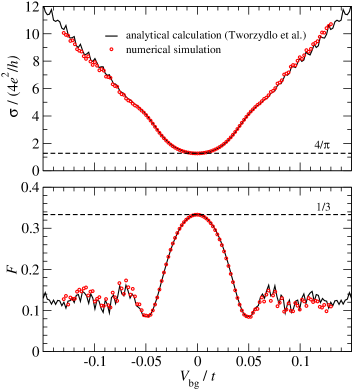
Refer to caption
Figure 10: Results of linear transport calculations for clean graphene sheets: Conductivity (defined as σ=LG/W𝜎𝐿𝐺𝑊\sigma=LG/W) and Fano factor as a function of the Fermi energy in the contacts (Vg=0subscript𝑉𝑔0V_{g}=0). The band in the square lattice leads was offset such that its middle coincides with the neutrality point in the graphene sheet in order to increase the density of states at the contact and thus mimic a metallic lead. Armchair edges, M=360𝑀360M=360 and N=70𝑁70N=70 (aspect ratio W/L=5.2𝑊𝐿5.2W/L=5.2).

9.1 Ballistic transport in clean samples

Here we present results obtained for the case of ballistic transport in graphene sheets. We consider mainly the armchair orientation, since this, in the clean limit, provides a band structure and dispersion relation very similar to a quasi-one-dimensional projection of the Dirac fermion model and is more suitable for scaling analyzes.

First, in Fig. 10, we show results for the clean limit (no bulk or edge disorder) for a short ribbon, keeping the back gate voltage fixed to zero (neutrality point) and varying the Fermi energy in the contacts (zero bias). The numerical data is compared to the analytical expressions derived by in Ref. Tworzydlo06 . The agreement is quite good for large systems and becomes worse when the system is too small (not shown). In particular, a strong asymmetry and a lack of well-defined oscillations occurs if the system is not large enough (not shown).
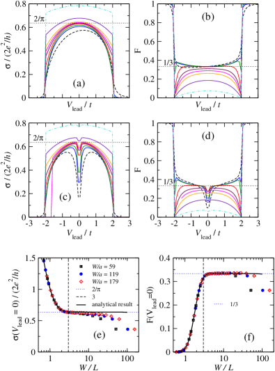
Refer to caption
Figure 11: Results of numerical simulations of clean ribbons: conductivity and Fano factor as a function of the Fermi energy in the contacts (Vg=0subscript𝑉𝑔0V_{g}=0) for different aspect ratios. (a), (b), (e), (f): Square lattice contacts; (c) and (d): Armchair honeycomb contacts. For all plots, M=120𝑀120M=120. In plots (a), (b), (c), and (d), the value of N𝑁N are 12 (dashed line), 24, 36, 72, 96, 108, 120, 148, and 200 (dashed-dotted line). The thick solid line corresponds to the analytical result Tworzydlo06 .

The ability of the recursive method to get precise results for clean systems is clear also in Fig. 11, where the calculations are performed for different aspect ratios. The deviations from the analytical curve only occur when the system is too short and evanescent modes dominate transport.
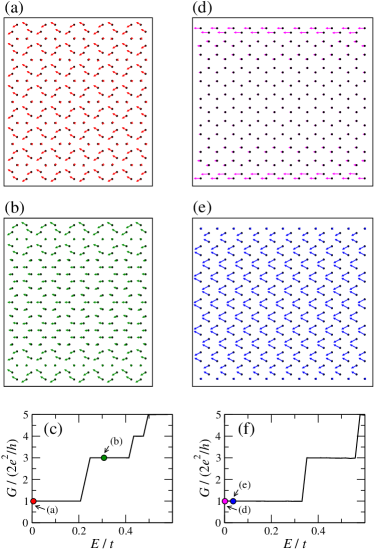
Refer to caption
Figure 12: Current densities (a,b,d,e) and linear conductance steps (c,d) of two small ballistic graphene ribbons. In (a,b,c,d) the arrows represent the current densities (in arbitrary units) evaluated at different sites using Eq. (112). Armchair edges, M=12𝑀12M=12, N=20𝑁20N=20: (a), (b), and (c); zigzag edges, M=12𝑀12M=12, N=21𝑁21N=21: (d), (e), and (f). Energies: E=0𝐸0E=0 for plots (a) and (d); E=0.3t𝐸0.3𝑡E=0.3t for plot (b); E=0.01t𝐸0.01𝑡E=0.01t for plot (e). amplitude.

In Figs. 12 we show the conductance and the current density in the linear regime for small flakes with armchair and zigzag edges. Here, the leads are also honeycomb lattices. In this case, the conductance steps can be easily understood from the energy dispersion relation of graphene infinite ribbons Brey06 , namely, the dimensionless conductance G/(2e2/h)𝐺2superscript𝑒2G/(2e^{2}/h) is given by the number of bands crossing the Fermi energy E𝐸E.

There is no such simple explanation for the current density. Notice that the notable difference in the current distribution for armchair and zigzag orientations at E=0𝐸0E=0: While in the latter the current is primarily carried by edge states, in the former the current is uniformly distributed across the flake. As one moves a just little bit away from E=0𝐸0E=0, the current distribution for the zigzag flake changes drastically, with nearly no current running at the edges. This result is related to the the fact that for zigzag nanoribbons the E=0𝐸0E=0 states are strongly localized at the edges. As soon as |E|>0𝐸0|E|>0 both edge states and edge currents disappear, even in the case of a single conducting channel. For the armchair orientation, the change in the current distribution for increasing energies is less drastic.

It should be stressed the edge current densities of zigzag nanoribbons change both quantitative and qualitative if one switches from nearest-neighbor Nikolic07 to next-nearest-neighbor tight-binding models Nikolic12 . The issue of which model is appropriate is tied to the desire to fit DFT calculations Son06 or to explain experimental manipulation and characterization of nanoribbon edges Tao11 .

9.2 Disordered graphene sheets

The conductivity minimum σ0subscript𝜎0\sigma_{0} observed at the charge neutrality point in graphene monolayers has been a subject of intense debate, which is reviewed, for instance, in Ref. Mucciolo10 . Here, we show how the long-range Gaussian correlated potential can be used to investigate the value of σ0subscript𝜎0\sigma_{0}. 444The discussion and results that follow complement the material presented in Ref. Mucciolo10 .

In the diffusive regime, in general, the system geometry has little influence on the transport properties which allows one to express the average conductivity as σ=(L/W)G𝜎𝐿𝑊delimited-⟨⟩𝐺\sigma=(L/W)\langle G\rangle, where L𝐿L is the system length and W𝑊W its width. We use the same setting as in the previous subsection, including now long-range Gaussian disorder in the device region. To generate the data shown in Fig. 13, four different aspect ratios were considered as well as several values of K0subscript𝐾0K_{0} and ξ/a𝜉𝑎\xi/a. The average conductivity σ0subscript𝜎0\sigma_{0} obtained from G(Vg=0)delimited-⟨⟩𝐺subscript𝑉𝑔0\langle G(V_{g}=0)\rangle is plotted versus L𝐿L scaled by superscript\ell^{*}. The parameter superscript\ell^{*} depends on K0subscript𝐾0K_{0} and ξ𝜉\xi. We identify superscript\ell^{*} with the elastic disorder mean free path \ell.

Refer to caption
Figure 13: Conductivity minimum σ0subscript𝜎0\sigma_{0} in unit of 2e2/h2superscript𝑒22e^{2}/h as a function of the system size L𝐿L scaled by the electron mean free path \ell. The results correspond to the average over 102104superscript102superscript10410^{2}\cdots 10^{4} disorder realizations for L𝐿L ranging between 50 and 500 a0subscript𝑎0a_{0}. The colors represent different aspect ratios W/L𝑊𝐿W/L. The symbols stand for the values of the dimensionless disorder strength K0subscript𝐾0K_{0}. The arrows indicate the analytical value of the conductivity minimum in the ballistic limit Tworzydlo06 , which depends on W/L𝑊𝐿W/L. The dotted line gives the diffusive ln(L/)𝐿\ln(L/\ell) behavior Ostrovsky06 .

Let us summarize the results shown in Fig. 13. Two clear regimes can be identified. For L/1much-less-than𝐿1L/\ell\ll 1, the probability of an electron being scattered by disorder as it traverses the sample is very small. This corresponds to the ballistic regime, where scattering occurs mainly at the sample edges and transport properties are dominated by the sample geometry. Note that when L/<1𝐿1L/\ell<1, σ0subscript𝜎0\sigma_{0} approaches the prediction for the pure ballistic case Tworzydlo06 , indicated by the arrows in Fig. 13. In contrast, when L/1much-greater-than𝐿1L/\ell\gg 1, the system becomes diffusive and geometry affects transport weakly. Figure 13 clearly shows this crossover. For the diffusive regime, L/l1much-greater-than𝐿𝑙1L/l\gg 1, the conductivity is proportional to ln(L/)𝐿\ln(L/\ell), in agreement with the non-linear sigma model prediction Ostrovsky06 . The mismatch between the numerical prefactor for the logarithm and the value characteristic of the symplectic class may be related to the finite contact resistance Adam09 present in our simulations.

These simulations suggest an explanation for results obtained in transport experiments at the charge neutrality point. In the coherent diffusive regime, the conductivity minimum has significant sample-to-sample fluctuations and its average shows a weak (logarithmic) dependence on the mean free path. Typical diffusive experimental samples have L/110𝐿110L/\ell\approx 1-10 and σ04e2/hsubscript𝜎04superscript𝑒2\sigma_{0}\approx 4e^{2}/h, similarly to what is shown in Fig. 13.
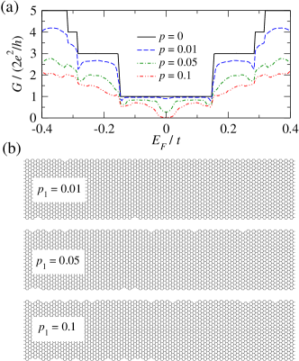
Refer to caption
Figure 14: (a) Linear conductance of edge disordered nanoribbons with armchair edge orientation, M=18𝑀18M=18, N=200𝑁200N=200, averaged over 100 realizations, as a function of energy. Only one etching sweep is used, but results for three different values of the site removal probability p1subscript𝑝1p_{1} are shown. (b) Typical realizations used in (a) for value of p1subscript𝑝1p_{1} considered.

9.3 Nanoribbons

For nanoribbons, both bulk and edge disorder play a role in electronic transport. In the absence of band gaps, long-range disorder does not suppress conductance significantly and a perfect conducting channel exists near the neutrality point Wakabayashi07 ; Wakabayashi09 ; Lima12 . The story is quite different for short-range disorder. Bulk imperfections (lattice defects, impurities, or adsorbates) and edge imperfections can lead to strong localization due to backscattering and enhanced destructive interference Evaldsson08 ; Mucciolo09 . To illustrate this point, Fig. 14 shows the rapid smearing of the linear conductance steps of a nanoribbon when even a small amount of edge sites are randomly removed (i.e., etched out). This shows how challenging it is to observe conductance quantization experimentally in these systems.
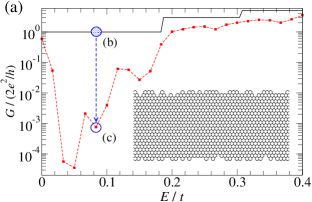
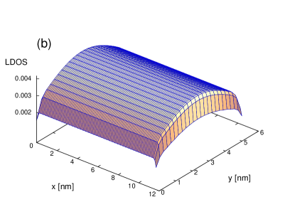
Refer to caption
Refer to caption
Refer to caption
Figure 15: (a) The linear conductance of a short nanoribbon (zigzag edges, M=24𝑀24M=24, N=91𝑁91N=91 sites) as a function of energy. The solid line corresponds to perfect edges while the dashed line corresponds to the edge disorder realization shown in the inset (three etching sweeps with p1=0.3subscript𝑝10.3p_{1}=0.3, p2=0.2subscript𝑝20.2p_{2}=0.2, p3=0.1subscript𝑝30.1p_{3}=0.1). Surface plot of the local density of states (arbitrary units, brickwall lattice representation) for the same nanoribbon at the energy value highlighted in (a): (b) clean case; (c) edge disordered case. Notice the appearance of localized states that traverse the nanoribbon when edge disorder is present. (The actual LDOS was convoluted with a Gaussian profile to smooth out high-frequency oscillations.)

The appearance of localized states in nanoribbons with edge disorder is demonstrated in Fig. 15 where the linear conductance and the local density of states for a nanoribbon are shown in the cases of perfect and irregular edges.

Acknowledgements.
Financial support by the Brazilian funding agencies FAPERJ and CNPq is gratefully acknowledged.

Appendix A Steps in the linear conductance

Let us show that the surface Green’s function in Eq. (67) leads to the expect steps in the linear conductance. For this purpose, let us begin by noticing that, in the case of a square lattice lead, only propagating modes yield a finite level width: For |Eεν|<2tx𝐸subscript𝜀𝜈2subscript𝑡𝑥|E-\varepsilon_{\nu}|<2t_{x},

Γ~ν=2Im[Σ~ν]=2Im[(g~ν)1]=2txsinϕν,subscript~Γ𝜈2Imdelimited-[]subscript~Σ𝜈2Imdelimited-[]superscriptsubscript~𝑔𝜈12subscript𝑡𝑥subscriptitalic-ϕ𝜈\tilde{\Gamma}_{\nu}=-2\,\mbox{Im}\left[\tilde{\Sigma}_{\nu}\right]=2\,\mbox{Im}\left[\left(\tilde{g}_{\nu}\right)^{-1}\right]=2\,t_{x}\,\sin\phi_{\nu}, (232)

where sinϕν=1(Eεν)2/4t2subscriptitalic-ϕ𝜈1superscript𝐸subscript𝜀𝜈24superscript𝑡2\sin\phi_{\nu}=\sqrt{1-(E-\varepsilon_{\nu})^{2}/4t^{2}}, in which case we can write g~ν=eiϕν/txsubscript~𝑔𝜈superscript𝑒𝑖subscriptitalic-ϕ𝜈subscript𝑡𝑥\tilde{g}_{\nu}=e^{-i\phi_{\nu}}/t_{x}.

In order to obtain the retarded Green’s function across the system, we add one slice between the left and right contacts and use the following expression, easily derivable from Eqs. (32), (33), (3.4) and (42):

G0,2=tx2gL2(gL1tx2gL)1subscript𝐺02superscriptsubscript𝑡𝑥2superscriptsubscript𝑔𝐿2superscriptsuperscriptsubscript𝑔𝐿1superscriptsubscript𝑡𝑥2subscript𝑔𝐿1G_{0,2}=t_{x}^{2}\,g_{L}^{2}\left(g_{L}^{-1}-t_{x}^{2}\,g_{L}\right)^{-1} (233)

Since G0,2subscript𝐺02G_{0,2} depends solely on gLsubscript𝑔𝐿g_{L}, we can rewrite in the propagation mode basis, in which case the Landauer formula is reduced to [see Eq. (15)]

𝒯=νΓ~ν(G~0,2)νΓ~ν(G~0,2)ν,𝒯superscriptsubscript𝜈subscript~Γ𝜈subscriptsubscript~𝐺02𝜈subscript~Γ𝜈superscriptsubscriptsubscript~𝐺02𝜈{\cal T}={\sum_{\nu}}^{\prime}\,\tilde{\Gamma}_{\nu}\,\left(\tilde{G}_{0,2}\right)_{\nu}\,\tilde{\Gamma}_{\nu}\,\left(\tilde{G}_{0,2}\right)_{\nu}^{\ast}, (234)

where the prime indicates that the sum runs only over states such that |Eεν|<2tx𝐸subscript𝜀𝜈2subscript𝑡𝑥|E-\varepsilon_{\nu}|<2t_{x} and

(G~0,2)ν=tx2g~ν2(g~ν1tx2g~ν)1=e2iϕν2itxsinϕν.subscriptsubscript~𝐺02𝜈superscriptsubscript𝑡𝑥2superscriptsubscript~𝑔𝜈2superscriptsuperscriptsubscript~𝑔𝜈1superscriptsubscript𝑡𝑥2subscript~𝑔𝜈1superscript𝑒2𝑖subscriptitalic-ϕ𝜈2𝑖subscript𝑡𝑥subscriptitalic-ϕ𝜈\left(\tilde{G}_{0,2}\right)_{\nu}=t_{x}^{2}\,\tilde{g}_{\nu}^{2}\left(\tilde{g}_{\nu}^{-1}-t_{x}^{2}\,\tilde{g}_{\nu}\right)^{-1}=\frac{e^{-2i\phi_{\nu}}}{2i\,t_{x}\,\sin\phi_{\nu}}. (235)

Putting all together, we find that

𝒯=𝒯absent\displaystyle{\cal T}= νΓ~ν2|(G~0,2)ν|2superscriptsubscript𝜈superscriptsubscript~Γ𝜈2superscriptsubscriptsubscript~𝐺02𝜈2\displaystyle{\sum_{\nu}}^{\prime}\;\tilde{\Gamma}_{\nu}^{2}\,\left|\left(\tilde{G}_{0,2}\right)_{\nu}\right|^{2}
=\displaystyle= ν 1=#propagatingmodesforagivenE,superscriptsubscript𝜈1#propagatingmodesforagiven𝐸\displaystyle{\sum_{\nu}}^{\prime}\;1=\#\ {\rm propagating\ modes\ for\ a\ given}\ E, (236)

which is the expected result for a clean ballistic system.

Appendix B Peierls hopping phases

Here we evaluate the phase of the hopping matrix elements between any two arbitrary sites due to the presence of a perpendicular magnetic field. We pick the vector potential in the generic Landau gauge Ax=(α1)Bysubscript𝐴𝑥𝛼1𝐵𝑦A_{x}=(\alpha-1)By and Ay=αBxsubscript𝐴𝑦𝛼𝐵𝑥A_{y}=\alpha Bx, with 0α10𝛼10\leq\alpha\leq 1. The (directional) Peierls phase between two neighboring sites k𝑘k and ksuperscript𝑘k^{\prime} is given by peierls

φk,ksubscript𝜑𝑘superscript𝑘\displaystyle\varphi_{k,k^{\prime}} =\displaystyle= eckk𝐀𝑑𝐥𝑒𝑐Planck-constant-over-2-pisuperscriptsubscript𝑘superscript𝑘𝐀differential-d𝐥\displaystyle\frac{ec}{\hbar}\int_{k}^{k^{\prime}}{\bf A}\cdot d{\bf l} (237)
=\displaystyle= ecB[(1α)cosθkkykyky𝑑l+αsinθkkxkxkx𝑑l]𝑒𝑐𝐵Planck-constant-over-2-pidelimited-[]1𝛼subscript𝜃𝑘superscript𝑘superscriptsubscriptsubscript𝑦𝑘subscript𝑦superscript𝑘𝑦differential-d𝑙𝛼subscript𝜃𝑘superscript𝑘superscriptsubscriptsubscript𝑥𝑘subscript𝑥superscript𝑘𝑥differential-d𝑙\displaystyle\frac{ecB}{\hbar}\left[(1-\alpha)\cos\theta_{kk^{\prime}}\int_{y_{k}}^{y_{k^{\prime}}}y\,dl+\alpha\sin\theta_{kk^{\prime}}\int_{x_{k}}^{x_{k^{\prime}}}x\,dl\right]
=\displaystyle= ecB[(1α)cotanθkkykyky𝑑y+αtanθkkxkxkx𝑑x]𝑒𝑐𝐵Planck-constant-over-2-pidelimited-[]1𝛼cotansubscript𝜃𝑘superscript𝑘superscriptsubscriptsubscript𝑦𝑘subscript𝑦superscript𝑘𝑦differential-d𝑦𝛼subscript𝜃𝑘superscript𝑘superscriptsubscriptsubscript𝑥𝑘subscript𝑥superscript𝑘𝑥differential-d𝑥\displaystyle\frac{ecB}{\hbar}\left[(1-\alpha)\,\mbox{cotan}\,\theta_{kk^{\prime}}\int_{y_{k}}^{y_{k^{\prime}}}y\,dy+\alpha\tan\theta_{kk^{\prime}}\int_{x_{k}}^{x_{k^{\prime}}}x\,dx\right]
=\displaystyle= ecB[(1α)(xkxk)(yk+yk2)\displaystyle\frac{ecB}{\hbar}\left[(1-\alpha)(x_{k^{\prime}}-x_{k})\left(\frac{y_{k^{\prime}}+y_{k}}{2}\right)\right.
+α(ykyk)(xk+xk2)],\displaystyle\hskip 31.2982pt\left.+\alpha(y_{k^{\prime}}-y_{k})\left(\frac{x_{k^{\prime}}+x_{k}}{2}\right)\right],

where θkksubscript𝜃𝑘superscript𝑘\theta_{kk^{\prime}} is the angle that the segment k𝑘kksuperscript𝑘k^{\prime} makes with the x𝑥x axis.

Notice that φk,k=φk,ksubscript𝜑𝑘superscript𝑘subscript𝜑superscript𝑘𝑘\varphi_{k,k^{\prime}}=-\varphi_{k^{\prime},k}. If we sum over all the bond phases around the perimeter of a hexagon, we obtain φ=3ecBa02/2=2π(Φ/Φ0)𝜑3𝑒𝑐𝐵superscriptsubscript𝑎022Planck-constant-over-2-pi2𝜋ΦsubscriptΦ0\sum\varphi=\sqrt{3}ecBa_{0}^{2}/2\hbar=2\pi\,(\Phi/\Phi_{0}), where Φ0=h/ecsubscriptΦ0𝑒𝑐\Phi_{0}=h/ec (flux quantum), and Φ=BAhexΦ𝐵subscript𝐴hex\Phi=B\,A_{\rm hex}, with Ahex=3a02/2subscript𝐴hex3superscriptsubscript𝑎022A_{\rm hex}=\sqrt{3}\,a_{0}^{2}/2 being the area of the hexagon.

Appendix C Random Flux Estimate

Let us estimate the rms value of the random magnetic field produced by the random vector potential:

B2delimited-⟨⟩superscript𝐵2\displaystyle\left\langle B^{2}\right\rangle =\displaystyle= (xAyyAx)2delimited-⟨⟩superscriptsubscript𝑥subscript𝐴𝑦subscript𝑦subscript𝐴𝑥2\displaystyle\left\langle(\partial_{x}A_{y}-\partial_{y}A_{x})^{2}\right\rangle (238)
=\displaystyle= {f𝒞k[ckx2(xn,jXk)ξ2+cky2(yn,jYk)ξ2]e|𝐫n,j𝐑k|2/ξ2}2delimited-⟨⟩superscript𝑓𝒞subscript𝑘delimited-[]subscriptsuperscript𝑐𝑥𝑘2subscript𝑥𝑛𝑗subscript𝑋𝑘superscript𝜉2subscriptsuperscript𝑐𝑦𝑘2subscript𝑦𝑛𝑗subscript𝑌𝑘superscript𝜉2superscript𝑒superscriptsubscript𝐫𝑛𝑗subscript𝐑𝑘2superscript𝜉22\displaystyle\left\langle\left\{\frac{f}{\cal C}\sum_{k}\left[c^{x}_{k}\frac{2(x_{n,j}-X_{k})}{\xi^{2}}+c^{y}_{k}\frac{2(y_{n,j}-Y_{k})}{\xi^{2}}\right]\,e^{-|{\bf r}_{n,j}-{\bf R}_{k}|^{2}/\xi^{2}}\right\}^{2}\right\rangle
=\displaystyle= 4f2𝒞2ξ4k|𝐫n,j𝐑k|2e2|𝐫n,j𝐑k|2/ξ24superscript𝑓2superscript𝒞2superscript𝜉4subscript𝑘superscriptsubscript𝐫𝑛𝑗subscript𝐑𝑘2superscript𝑒2superscriptsubscript𝐫𝑛𝑗subscript𝐑𝑘2superscript𝜉2\displaystyle\frac{4f^{2}}{{\cal C}^{2}\xi^{4}}\sum_{k}|{\bf r}_{n,j}-{\bf R}_{k}|^{2}\,e^{-2|{\bf r}_{n,j}-{\bf R}_{k}|^{2}/\xi^{2}}
\displaystyle\approx 4f2𝒞2ξ4ag2d2RR2e2R2/ξ24superscript𝑓2superscript𝒞2superscript𝜉4superscriptsubscript𝑎𝑔2superscript𝑑2𝑅superscript𝑅2superscript𝑒2superscript𝑅2superscript𝜉2\displaystyle\frac{4f^{2}}{{\cal C}^{2}\xi^{4}a_{g}^{2}}\int d^{2}R\,R^{2}\,e^{-2R^{2}/\xi^{2}}
\displaystyle\approx πf22𝒞2ag2=f2ag22πξ4.𝜋superscript𝑓22superscript𝒞2superscriptsubscript𝑎𝑔2superscript𝑓2superscriptsubscript𝑎𝑔22𝜋superscript𝜉4\displaystyle\frac{\pi\,f^{2}}{2\,{\cal C}^{2}a_{g}^{2}}=\frac{f^{2}a_{g}^{2}}{2\pi\,\xi^{4}}.

References

  • (1) Castro Neto, A. H. F. Guinea, F., Peres, N. M. R. , Novoselov, K. S., Geim, A. K.: The electronic properties of graphene. Rev. Mod. Phys. 81, 109 (2009)
  • (2) Mucciolo, E.R., Lewenkopf, C.H.: Disorder and electronic transport in graphene. J. Phys.: Condens. Matter 22, 273201 (2010)
  • (3) Shon N.H., Ando, T.: Quantum transport in two-dimensional graphite system. J. Phys. Soc. Jap. 67, 2421 (1998)
  • (4) Ostrovsky, P.M., Gornyi, I.V., Mirlin, A.D.; Electron transport in disordered graphene. Phys. Rev. B 74 235443 (2006)
  • (5) Nomura K., MacDonald, A. H.: Quantum transport of massless Dirac fermions. Phys. Rev. Lett. 98, 076602 (2007)
  • (6) Nomura, K., Koshino, M., Ryu, S.: Topological delocalization of two-dimensional massless Dirac fermions. Phys. Rev. Lett. 99, 146806 (2007)
  • (7) Tworzydło, J., Groth, C.W., Beenakker, C.W.J.: Finite difference method for transport properties of massless Dirac fermions. Phys. Rev. B 78, 235438 (2008)
  • (8) Hernández, A.R., Lewenkopf, C.H.: Finite-difference method for transport of two-dimensional massless Dirac fermions in a ribbon geometry, Phys. Rev. B 86, 155439 (2012)
  • (9) Thouless, D.J., Kirkpatrick, S.: Conductivity of the disordered linear chain. J. Phys. C 14, 235 (1981)
  • (10) Drouvelis, P. S., Schmelcher, P., Bastian, P.: Parallel implementation of the recursive Green’s function method. J. Comp. Phys. 215, 741 (2006)
  • (11) MacKinnon, A: The calculation of transport properties and density of states of disordered solids. Z. Phys. B 59, 385 (1985)
  • (12) Sols, F, Macucci, M., Ravaioli, U., Hess, K.: Theory for a quantum modulated transistor. J. Appl. Phys. 66, 3892 (1989)
  • (13) Baranger, H.U., DiVincenzo, D.P., Jalabert, R.A., Stone, A.D.: Classical and quantum ballistic-transport anomalies in microjunctions. Phys. Rev. B 44, 10637 (1991)
  • (14) Kazymyrenko, K., Waintal, X.: Knitting algorithm for calculating Green functions in quantum systems. Phys. Rev. B 77, 115119 (2008)
  • (15) Kramer, T., Kreisbeck, C., Krueckl, V.: Wave-packet dynamics approach to transport in mesoscopic systems. Phys. Scr. 82, 038101 (2010)
  • (16) Yuan, S., De Raedt, H., Katsnelson, M.I.: Modeling electronic structure and transport properties of graphene. with resonant scattering centers Phys. Rev. B 82 115448 (2010)
  • (17) Weiße, A., Wellein, G., Alvermann A., Fehske, H.: The kernel polynomial method. Rev. Mod. Phys. 78, 275 (2006)
  • (18) Ferreira, A., Viana-Gomes, J., Nilsson, J., Mucciolo, E. R., Peres, N.M.R., Castro Neto, A.H.: Unified description of the dc conductivity of monolayer and bilayer graphene at finite densities based on resonant scatterers Phys. Rev. B 83, 165402 (2011)
  • (19) Triozon, F., Roche, S.: Efficient linear scaling method for computing the Landauer-Büttiker conductance. Eur. Phys. J. B 46, 427 (2005)
  • (20) Liu M.-H., Richter, K.: Efficient quantum transport simulation for bulk graphene heterojunctions. Phys. Rev. B 86 115445 (2012)
  • (21) Datta, S.: Electronic Transport in Mesoscopic Systems. Cambridge University Press, Cambridge (1996)
  • (22) Ferry, D.K., Goodnick, S.M.: Transport in Nanostructures. Cambridge University Press, Cambridge (1997)
  • (23) Landauer, R.: Spatial variation of currents and fields due to localized scatterers in metallic conduction. IBM J. Res. Develop. 32, 306 (1988)
  • (24) Caroli, C., Combescot, R., Nozieres, P., Saint-James, D.: Direct calculation of the tunneling current. J. Phys. C 4, 916 (1971)
  • (25) Lee, P.A., Fisher, D.S.: Anderson localization in two dimensions. Phys. Rev. Lett. 47, 882 (1981)
  • (26) Fisher, D. S., Lee, P. A.: Relation between conductivity and transmission matrix. Phys. Rev. B 23, 6851 (1981)
  • (27) Sajjad, R.N., Polanco, C., Ghosh, A.W.: Atomistic deconstruction of current flow in graphene based hetero-junctions. arXiv:1302.4473 (2013)
  • (28) Meir, Y., Wingreen, N.S.: Landauer formula for the current through an interacting electron region. Phys. Rev. Lett. 68, 2512 (1992)
  • (29) Hernández, A., Apel V.M., Pinheiro, F.A., Lewenkopf, C.H.: Quantum electronic transport: Linear and nonlinear conductance from the Keldysh approach. Physica A 385, 148 (2007)
  • (30) Lewenkopf, C.H., Mucciolo, E.R., Castro Neto, A.H.: Numerical studies of conductivity and Fano factor in disordered graphene. Phys. Rev. B 77, 081410R (2008)
  • (31) Haug, H., Jauho A.-P.: Quantum kinetics in transport and optics of semiconductors, 2nd Edition. Springer, Heidelberg (2008)
  • (32) Mucciolo, E.R.: unpublished
  • (33) Schomerus, H.: Effective contact model for transport through weakly-doped graphene. Phys. Rev. B 76, 045433 (2007)
  • (34) Areshkin, D. A., Nikolić, B. K.: IV𝐼𝑉I-V curve signatures of nonequilibrium-driven band gap collapse in magnetically ordered zigzag graphene nanoribbon two-terminal devices. Phys. Rev. B 79, 205430 (2009)
  • (35) Lopez Sancho M.P., Lopez Sancho J.M., Rubio J.: Highly convergent schemes for the calculation of bulk and surface Green functions. J. Phys. F: Met. Phys. 15, 851 (1985)
  • (36) Umerski, A.: Closed-form solutions to surface Green’s functions. Phys. Rev. B 55, 5266 (1997)
  • (37) Rocha, A.R., García-Suárez, V.M., Bailey, S., Lambert, C., Ferrer, J., Sanvito S.: Spin and molecular electronics in atomically generated orbital landscapes. Phys. Rev. B 73, 085414 (2006)
  • (38) Wimmer, M.: Quantum transport in nanostructures: From computational concepts to spintronics in graphene and magnetic tunnel junctions. http://epub.uni-regensburg.de/12142/, Dissertation, University Regensburg (2009)
  • (39) Tworzydło, J., Trauzettel, B., Titov, M., Rycerz, A., Beenakker, C.W.J.: Sub-poissonian shot noise in graphene. Phys. Rev. Lett. 96, 246802 (2006); supplementary material is found in cond-mat/0603315.
  • (40) Rycerz, A., Tworzydło, J., Beenakker, C.W.J.: Anomalously large conductance fluctuations in weakly disordered graphene. Europhys. Lett. 79, 57003 (2007)
  • (41) Metalidis, G., Bruno, P.: Green’s function technique for studying electron flow in two-dimensional mesoscopic samples. Phys. Rev. B 72, 235304 (2005)
  • (42) Todorov, T. N.: Tight-binding simulation of current-carrying nanostructures. J. Phys.: Condens. Matter 14, 3049 (2002).
  • (43) Cresti, A., Farchioni, R., Grosso, G., Parravicini, G. P.: Keldysh-Green function formalism for current profiles in mesoscopic systems. Phys. Rev. B 68, 075306 (2003)
  • (44) Yazyev, O.: Emergence of magnetism in graphene materials and nanostructures. Rep. Prog. Phys. 73, 056501 (2010)
  • (45) Son, Y.W., Cohen, M.L., Louie, S.G.: Energy gaps in graphene nanoribbons. Phys. Rev. Lett. 97, 216803 (2006)
  • (46) Xue, Y., Datta, S., Ratner, M.A.: First-principles based matrix Green’s function approach to molecular electronic devices: general formalism. Chem. Phys. 281, 151 (2002)
  • (47) Areshkin, D. A., Nikolić, B. K.: Electron density and transport in top-gated graphene nanoribbon devices: First-principles Green function algorithms for systems containing a large number of atoms. Phys. Rev. B 81, 155540 (2010)
  • (48) Bruus H., Flensberg, K.: Many-Body Quantum Theory in Condensed Matter Physics: An Introduction. Oxford University Press, New York (2004)
  • (49) Nazarov, Y. V., Blanter, Y. M.: Quantum Transport: Introduction to Nanoscience. Cambridge University Press, New York (2009)
  • (50) Büttiker, M.: Coherent and sequential tunneling in series barriers. IBM J. Res. Developm. 32, 63 (1988)
  • (51) D’Amato, J.L., Pastawski, H.M.: Conductance of a disordered linear chain including inelastic scattering events. Phys. Rev. B 41, 7411 (1990)
  • (52) Martin, J., Akerman, N., Ulbricht, G., Lohmann, T., Smet, J.H., von Klitzing, K., Yacoby, A.: Observation of electron-hole puddles in graphene using a scanning single electron transistor. Nature Phys. 4, 144 (2008)
  • (53) Zhang, Y., Brar, V.W., Girit, C., Zettl, A., Crommie, M.F.: Origin of spatial charge inhomogeneity in graphene. Nature Phys. 5, 722 (2009)
  • (54) Ishigami, M., Chen, J.H., Cullen, W.G., Fuhrer, M.S., Williams, E.D.: Atomic structure of graphene on SiO2. Nano Lett. 7, 1643 (2007)
  • (55) Meyer, J.C., Geim, A.K., Katsnelson, M.I., Novoselov, K.S., Obergfell, D., Roth, S., Girit, Ç., Zettl, A.: On the roughness of single- and bi-layer graphene membranes. Solid State Comm. 143, 101 (2007)
  • (56) Levy, N., Burke, S.A. Meaker, K.L., Panlasigui, M., Zettl, A., Guinea, F., Castro Neto, A.H., Crommie, M.F.: Strain-induced pseudo-magnetic fields greater than 300 Tesla in graphene nanobubbles. Science 329, 544 (2010)
  • (57) Chen, J.H., Jang, C., Adam, S., Fuhrer, M.S., Williams, E.D., Ishigami, M.: Charged-impurity scattering in graphene. Nature Phys. 4, 377 (2008)
  • (58) Chen, J.-H., Cullen, W. G., Jang, C., Fuhrer, M. S., Williams, E. D.: Defect scattering in graphene. Phys. Rev. Lett. 102, 236805 (2009)
  • (59) Han, M., Brant, J.C., Kim, P.: Electron transport in disordered graphene nanoribbons. Phys. Rev. Lett. 104, 056801 (2010)
  • (60) Peres, N.M.R.: Colloquium: The transport properties of graphene: An introduction. Rev. Mod. Phys. 82, 2673 (2010)
  • (61) Das Sarma, S., Adam, S., Hwang, E. H., Rossi, E.: Electronic transport in two-dimensional graphene. Rev. Mod. Phys. 83, 407 (2011)
  • (62) Adam, S., Brouwer, P.W., Das Sarma, S.: Crossover from quantum to Boltzmann transport in graphene. Phys. Rev. B 79, 201404 (2009)
  • (63) Kłos, J.W., Zozoulenko, I.V.: Effect of short- and long range scattering on the conductivity of graphene: Boltzmann approach vs tight-binding calculations. Phys. Rev. B 82, 081414(R) (2010)
  • (64) Pereira V.M, Castro Neto, A. H., Peres, N.M.R.: Tight-binding approach to uniaxial strain in graphene. Phys. Rev. B 80, 045401 (2009)
  • (65) Landau, L.D., Lifshitz, E.M: Theory of elasticity, 3rd edition. Pergamon, London (1986)
  • (66) Kim, E.-A., Castro Neto A. H.: Graphene as an electronic membrane. Europhys. Lett. 84, 57007 (2008)
  • (67) Vozmediano, M.A.H., Katsnelson, M.I., Guinea, F.: Gauge fields in graphene. Phys. Rep. 496, 109 (2010)
  • (68) Peierls, R.E.: Zur Theorie des Diamagnetismus von Leitungselektronen. Z. Phys. 80, 763 (1933)
  • (69) Lundeberg, M.B., Folk, J.A.: Rippled graphene in an in-plane magnetic field: effects of a random vector potential. Phys. Rev. Lett. 105, 146804 (2010)
  • (70) Sols, F., Guinea, F., Castro Neto A.H.: Coulomb blockade in graphene nanoribbons. Phys. Rev. Lett. 99, 166803 (2007)
  • (71) Vérges, J.A., Guinea, F., Chiappe, G., Louis, E.: Transport regimes in surface disordered graphene sheets. Phys. Rev. B 75, 085440 (2007)
  • (72) Evaldsson, M., Zozoulenko, I.V., Xu, H., Heinzel, T.: Edge disorder induced Anderson localization and conduction gap in graphene nanoribbons. Phys. Rev. B 78, 161407(R) 2008
  • (73) Mucciolo, E.R., Castro Neto, A.H, Lewenkopf, C.H.: Conductance quantization and transport gaps in disordered graphene nanoribbons. Phys. Rev. B 79, 075407 (2009)
  • (74) Brey L., Fertig, H.A.: Electronic states of graphene nanoribbons studied with the Dirac equation. Phys. Rev. B 73, 235411 (2006)
  • (75) Zârbo, L.P., Nikolić, B.K.: Spatial distribution of local currents of massless Dirac fermions in quantum transport through graphene nanoribbons. EPL 80, 47001 (2007)
  • (76) Chang P.-H., Nikolić, B.K.: Edge currents and nanopore arrays in zigzag and chiral graphene nanoribbons as a route toward high-ZT thermoelectrics. Phys. Rev. B 86, 041406(R) (2012)
  • (77) Tao, C., Jiao, L., Yazyev, O.V., Chen, Y.-C., Feng, J., Zhang, X., Capaz, R.B., Tour, J.M., Zettl, A., Louie, S.G., Dai, H., Crommie, M.F.: Spatially resolving edge states of chiral graphene nanoribbons. Nature Phys. 7, 616 (2011)
  • (78) Wakabayashi, K., Takane, Y., Sigrist, M.: Perfectly conducting channel and universality crossover in disordered graphene nanoribbons. Phys. Rev. Lett. 99, 036601 (2007)
  • (79) Wakabayashi, K., Takane, Y.,Yamamoto, M., Sigrist, M.: Electronic transport properties of graphene nanoribbons. New J. Phys. 11, 095016 (2009)
  • (80) Lima, L.R.F., Pinheiro, F.A., Capaz, R.B., Lewenkopf, C.H., Mucciolo, E.R.: Effects of disorder range and electronic energy on the perfect transmission in graphene nanoribbons. Phys. Rev. B 86, 205111 (2012)