Dijet azimuthal decorrelations at the LHC
in the parton Reggeization approach

Abstract

We study inclusive dijet azimuthal decorrelations in proton-proton collisions at the CERN LHC invoking the hypothesis of parton Reggeization in $t-$channel exchanges at high energies. In the parton Reggeization approach, the main contribution to the azimuthal angle difference between the two most energetic jets is due to the Reggeon-Reggeon-particle-particle scattering, when the fusion of two Reggeized gluons into a pair of Yang-Mills gluons dominates. Using a high-energy factorization scheme with the Kimber-Martin-Ryskin unintegrated parton distribution functions and the Fadin-Lipatov effective vertices we obtain good agreement of our calculations with recent measurements by the ATLAS and CMS Collaborations at the CERN LHC.

I Introduction

The production of large transverse-momentum ($p_{T}$) hadron jets at the high-energy colliders, like the Tevatron and the LHC, is reasonably considered as an important source of information about the dynamics of parton-parton interactions at small distances and parton distribution functions (PDF), and as a probe to test perturbative quantum chromodynamics (pQCD) Review . The measurements of decorrelations in the azimuthal angle between the two most energetic jets, $\Delta\varphi$, as a function of the number of produced jets, give the chance to separate directly leading-order (LO) and next-to-leading orders (NLO) contributions in the strong coupling constant $\alpha_{s}$. Furthermore, a precise understanding of the physics of events with large azimuthal decorrelations is essential for the search for new physical phenomena with dijet signatures by the CMS CMS2 and ATLAS ATLAS2 detectors at the LHC.

The total collision energies, $\sqrt{S}=7$ TeV or 14 TeV at the LHC, sufficiently exceed the transverse momenta of identified jets ($0.1<p_{T}<1.3$ TeV). The recent theoretical studies of single-jet production at very high energy show the dominance of the multi-Regge final states in the inclusive production cross sections KSSY . In other words, in the high-energy regime the contribution of partonic subprocesses involving $t-$channel parton exchanges become dominant. Then the transverse momenta of the incoming partons and their off-shell properties can no longer be neglected, and we deal with QCD-scattering amplitudes with Reggeized $t-$channel partons. As it has been shown by Lipatov and co-authors, Reggeized gluons and quarks are the appropriate gauge-invariant degrees of freedom of high-energy pQCD. In the practical applications, the use of Reggeized $t-$channel exchanges is justified by the dominance of the so-called multi-Regge final states in inelastic collisions of high-energy hadrons.

The parton Reggeization approach FadinLipatov ; FadinSherman is based on an effective quantum field theory implemented with the non-Abelian gauge-invariant action which includes fields of Reggeized gluons Lipatov95 and Reggeized quarks LipatoVyazovsky . Recently, this approach was successfully applied to interpret the $p_{T}-$spectra of inclusive production of a single jet KSSY , prompt photon tevatronY ; heraY , Drell-Yan lepton pairs NNS_DY and bottom-flavored jets bbTEV ; bbLHC at the Tevatron and LHC. The single-jet production is dominated by the multi-Regge kinematics (MRK), when only a jet with a highest transverse momentum (leading jet) is produced in the central rapidity region, being strongly separated in rapidity from other particles. If the same situation is realized for two or more the most energetic jets, then quasimulti-Regge kinematics (QMRK) is at work.

In the present paper we extend our analysis of inclusive single-jet production at the LHC based on the parton Reggeization approach to a case of dijet production, and study azimuthal decorrelations between the two central jets with the largest transverse momenta according to the measurements implemented by the CMS and ATLAS Collaborations CMS2 ; ATLAS2 .

This paper is organized as follows: In Sec. II, the parton Reggeization approach is briefly reviewed. We write down relevant Reggeon-Reggeon-particle-particle effective vertices, effective amplitudes, squared matrix elements and differential cross sections. In Sec. III, we present the results of our calculations for two-jet azimuthal decorrelation spectra and perform a comparison with corresponding experimental data from the CERN LHC at $\sqrt{S}=7$ TeV. Sec. IV contains our conclusions.

II Dijet production in QMRK

In the high-energy Regge limit, when the collision energy is very high but the transverse momenta of the produced jets are fixed by the condition $\sqrt{S}>>p_{T}>>\Lambda_{QCD}$, the high-energy (uncollinear) factorization works well instead of collinear parton model. In this case, the Balitsky-Fadin-Kuraev-Lipatov (BFKL) QCD evolution of unintegrated PDFs BFKL can be more adequate approximation than the Dokshtser-Gribov-Lipatov-Altarelli-Parisi (DGLAP) QCD evolution of collinear PDFs DGLAP . This means, that we need to consider the processes with strong ordering in rapidity at the MRK or QMRK conditions. We identify final-state jets and final-state partons, and consider the production of two partons in the central region of rapidity, assuming that there are no any other partons with the same rapidity. To the LO in the parton Reggeization approach we have the following partonic subprocesses, which describe the production of two central jets in proton-proton collisions:

$$R+R\to g+g,$$ (1)

$$R+R\to q+\bar{q},$$ (2)

$$Q+R\to q+g,$$ (3)

$$Q+Q\to q+q,$$ (4)

$$Q+Q^{\prime}\to q+q^{\prime},$$ (5)

$$Q+\bar{Q}\to q+\bar{q},$$ (6)

$$Q+\bar{Q}\to q^{\prime}+\bar{q}^{\prime},$$ (7)

$$Q+\bar{Q}\to g+g,$$ (8)

where $R$ is a Reggeized gluon, $Q$ is a Reggeized quark, $g$ is a Yang-Mills gluon, $q$ is an ordinary quark, $q$ and $q^{\prime}$ denote quarks of different flavors. Working in the center-of-mass (c.m.) frame, we write the four-momenta of the incoming protons as $P_{1,2}^{\mu}=(\sqrt{S}/2)(1,0,0,\pm 1)$ and those of the Reggeized partons as $q_{i}^{\mu}=x_{i}P_{i}^{\mu}+q_{iT}^{\mu}\ (i=1,2)$, where $x_{i}$ are longitudinal momentum fractions and $q_{iT}^{\mu}=(0,{\bf q}_{iT},0)$, with ${\bf q}_{iT}$ being transverse two-momenta, and we define $t_{i}=-q_{iT}^{2}={\bf q}_{iT}^{2}$. The final partons have four-momenta $k_{1,2}$ and they are on-shell and massless $k_{1}^{2}=k_{2}^{2}=0$.

The effective gauge-invariant amplitudes for the above-mentioned subprocesses (1)-(8) can be obtained using the effective Feynman rules from Refs.  Lipatov95 ; LipatoVyazovsky ; Antonov . As usual, we introduce the light-cone vectors $n^{+}=2P_{2}/\sqrt{S}$ and $n^{-}=2P_{1}/\sqrt{S}$, and define $k^{\pm}=k\cdot n^{\pm}$ for any four-vector $k^{\mu}$. Than we determine effective vertices:

$$\Gamma^{(+-)}_{\mu}(q_{1},q_{2}) = 2\left[\left(q_{1}^{+}+\frac{q_{1}^{2}}{q_{2}^{-}}\right)n^{-}_{\mu}-\left(q_{2}^{-}+\frac{q_{2}^{2}}{q_{1}^{+}}\right)n^{+}_{\mu}+(q_{2}-q_{1})_{\mu}\right],$$ (9)

$$\gamma_{\mu}^{\pm}(q,p) = \gamma_{\mu}+\hat{q}\frac{n^{\pm}_{\mu}}{p^{\pm}},$$ (10)

$$\gamma_{\mu}^{(+-)}(q_{1},q_{2}) = \gamma_{\mu}-\hat{q}_{1}\frac{n_{\mu}^{-}}{q_{2}^{-}}-\hat{q}_{2}\frac{n_{\mu}^{+}}{q_{1}^{+}},$$ (11)

$$\Gamma^{\mu\nu+}(q_{1},q_{2}) = 2q_{1}^{+}g^{\mu\nu}-(n^{+})^{\mu}(q_{1}-q_{2})^{\nu}-(n^{+})^{\nu}(q_{1}+2q_{2})^{\mu}+\frac{t_{2}}{q_{1}^{+}}(n^{+})^{\mu}(n^{+})^{\nu},$$

$$\Gamma^{\mu\nu-}(q_{1},q_{2}) = 2q_{2}^{-}g^{\mu\nu}+(n^{-})^{\mu}(q_{1}-q_{2})^{\nu}-(n^{-})^{\nu}(q_{2}+2q_{1})^{\mu}+\frac{t_{1}}{q_{2}^{-}}(n^{-})^{\mu}(n^{-})^{\nu},$$ (12)

and the triple-gluon vertex

$$\gamma_{\mu\nu\sigma}(q,p) = (q-p)_{\sigma}g_{\mu\nu}-(p+2q)_{\mu}g_{\nu\sigma}+(2p+q)_{\nu}g_{\mu\sigma}.$$ (13)

Finally, we can write the effective vertices for relevant subprocesses as follows:

$$C_{RR,ab}^{gg,~{}cd,~{}\mu\nu}(q_{1},q_{2},k_{1},k_{2}) = g_{s}^{2}\frac{q_{1}^{+}q_{2}^{-}}{4\sqrt{t_{1}t_{2}}}\biggl{(}T_{1}s^{-1}\Gamma^{(+-)_{\sigma}}(q_{1},q_{2})\gamma_{\mu\nu\sigma}(-k_{1},-k_{2})+$$ (14)

$$+ T_{3}t^{-1}\Gamma^{\sigma\mu-}(q_{1},k_{1}-q_{1})\Gamma^{\sigma\nu+}(k_{2}-q_{2},q_{2})-$$

$$- T_{2}u^{-1}\Gamma^{\sigma\nu-}(q_{1},k_{2}-q_{1})\Gamma^{\sigma\mu+}(k_{1}-q_{2},q_{2})-$$

$$- T_{1}\bigl{(}n^{-}_{\mu}n^{+}_{\nu}-n^{-}_{\nu}n^{+}_{\mu}\bigr{)}-T_{2}\bigl{(}2g_{\mu\nu}-n^{-}_{\mu}n^{+}_{\nu}\bigr{)}-T_{3}\bigl{(}-2g_{\mu\nu}+n^{-}_{\nu}n^{+}_{\mu}\bigr{)}+$$

$$+ \Delta^{\mu\nu+}(q_{1},q_{2},k_{1},k_{2})+\Delta^{\mu\nu-}(q_{1},q_{2},k_{1},k_{2})\biggr{)},$$

where

$$T_{1}=f_{cdr}f_{abr},\quad T_{2}=f_{dar}f_{cbr},\quad T_{3}=f_{acr}f_{dbr},\quad T_{1}+T_{2}+T_{3}=0,$$

$$\Delta^{\mu\nu+}(q_{1},q_{2},k_{1},k_{2})=2t_{2}n^{+}_{\mu}n^{+}_{\nu}\biggl{(}\frac{T_{3}}{k_{2}^{+}q_{1}^{+}}-\frac{T_{2}}{k_{1}^{+}q_{1}^{+}}\biggr{)},$$

$$\Delta^{\mu\nu-}(q_{1},q_{2},k_{1},k_{2})=2t_{1}n^{-}_{\mu}n^{-}_{\nu}\biggl{(}\frac{T_{3}}{k_{1}^{-}q_{2}^{-}}-\frac{T_{2}}{k_{2}^{-}q_{2}^{-}}\biggr{)},$$

$f^{abc}$ are structure constants of the color gauge group SU(3), $g_{s}^{2}=4\pi\alpha_{s}$, and $\alpha_{s}$ is a strong coupling constant.

$$C_{RR,~{}ab}^{q\bar{q}}(q_{1},q_{2},k_{1},k_{2}) = g_{s}^{2}\frac{q_{1}^{+}q_{2}^{-}}{4\sqrt{t_{1}t_{2}}}\bar{U}(k_{1})\left(-s^{-1}[T^{a},T^{b}]\gamma^{\sigma}\Gamma^{(+-)}_{\sigma}(q_{1},q_{2})+\right.$$ (15)

$$+ \left.t^{-1}T^{a}T^{b}\gamma^{-}(\hat{k}_{1}-\hat{q}_{1})\gamma^{+}+u^{-1}T^{b}T^{a}\gamma^{+}(\hat{k}_{1}-\hat{q}_{2})\gamma^{-}\right)V(k_{2}),$$

$$C_{QR,~{}a}^{qg,~{}b,~{}\mu}(q_{1},q_{2},k_{1},k_{2}) = \frac{1}{2}g_{s}^{2}\frac{q_{2}^{-}}{2\sqrt{t_{2}}}\bar{U}(k_{1})\biggl{[}\gamma_{\sigma}^{(-)}(q_{1},k_{1}-q_{1})t^{-1}\bigl{(}\gamma_{\mu\nu\sigma}(k_{2},-q_{2})n_{\nu}^{+}+t_{2}\frac{n_{\mu}^{+}n_{\sigma}^{+}}{k_{2}^{+}}\bigr{)}\times$$ (16)

$$\times \bigl{[}T^{a},T^{b}\bigr{]}-\gamma^{+}(\hat{q}_{1}-\hat{k}_{2})^{-1}\gamma_{\mu}^{(-)}(q_{1},-k_{2})T^{a}T^{b}-$$

$$- \gamma_{\mu}(\hat{q}_{1}+\hat{q}_{2})^{-1}\gamma_{\sigma}^{(-)}(q_{1},q_{2})n_{\sigma}^{+}T^{b}T^{a}+\frac{2\hat{q}_{1}n_{\mu}^{-}}{k_{1}^{-}}\biggl{(}\frac{T^{a}T^{b}}{k_{2}^{-}}-\frac{T^{b}T^{a}}{q_{2}^{-}}\biggr{)}\biggr{]},$$

$$C_{QQ}^{qq}(q_{1},q_{2},k_{1},k_{2}) = g_{s}^{2}\left(t^{-1}\bar{U}(k_{2})\gamma_{\sigma}^{(+)}(q_{2},k_{2}-q_{2})T^{c}\otimes\bar{U}(k_{1})\gamma_{\sigma}^{(-)}(q_{1},k_{1}-q_{1})T^{c}-\right.$$ (17)

$$- \left.u^{-1}\bar{U}(k_{1})\gamma_{\sigma}^{(+)}(q_{2},k_{1}-q_{2})T^{c}\otimes\bar{U}(k_{2})\gamma_{\sigma}^{(-)}(q_{1},k_{2}-q_{1})T^{c}\right),$$

$$C_{QQ^{\prime}}^{qq^{\prime}}(q_{1},q_{2},k_{1},k_{2})=g_{s}^{2}t^{-1}\bar{U}(k_{2})\gamma_{\sigma}^{(+)}(q_{2},k_{2}-q_{2})T^{c}\otimes\bar{U}(k_{1})\gamma_{\sigma}^{(-)}(q_{1},k_{1}-q_{1})T^{c},$$ (18)

$$C_{Q\bar{Q}}^{q\bar{q}}(q_{1},q_{2},k_{1},k_{2}) = g_{s}^{2}\left(s^{-1}\bar{U}(k_{1})\gamma_{\sigma}T^{c}V(k_{2})\otimes\gamma_{\sigma}^{(+-)}(q_{1},q_{2})T^{c}+\right.$$ (19)

$$+ \left.t^{-1}\bar{U}(k_{1})\gamma_{\sigma}^{(+)}(q_{2},k_{2}-q_{2})T^{c}\otimes\gamma_{\sigma}^{(-)}(q_{1},k_{1}-q_{1})T^{c}V(k_{2})\right),$$

$$C_{Q\bar{Q}}^{q^{\prime}\bar{q}^{\prime}}(q_{1},q_{2},k_{1},k_{2})=g_{s}^{2}s^{-1}\bar{U}(k_{1})\gamma_{\sigma}T^{c}V(k_{2})\otimes\gamma_{\sigma}^{(+-)}(q_{1},q_{2})T^{c},$$ (20)

$$C_{Q\bar{Q}}^{gg,~{}ab,~{}\mu\nu}(q_{1},q_{2},k_{1},k_{2}) = -g_{s}^{2}\biggl{(}\gamma_{\nu}^{(+)}(q_{2},-k_{2})(\hat{k}_{2}-\hat{q}_{2})^{-1}\gamma_{\mu}^{(-)}(q_{1},-k_{1})T^{b}T^{a}+$$ (21)

$$+ \gamma_{\nu}^{(+)}(q_{2},-k_{1})(\hat{k}_{1}-\hat{q}_{2})^{-1}\gamma_{\mu}^{(-)}(q_{1},-k_{2})T^{a}T^{b}+$$

$$+ \gamma_{\mu\nu\sigma}(-k_{1},-k_{2})s^{-1}\gamma^{(+-)}_{\sigma}(q_{1},q_{2})[T^{a},T^{b}]+\Delta_{\mu\nu}^{ab}(q_{1},q_{2})\biggr{)},$$

where

$$\Delta_{\mu\nu}^{ab}(q_{1},q_{2})=\frac{\hat{q}_{1}n_{\mu}^{-}n_{\nu}^{-}}{q_{2}^{-}}\biggl{(}\frac{T^{a}T^{b}}{k_{2}^{-}}+\frac{T^{b}T^{a}}{k_{1}^{-}}\biggr{)}-\frac{\hat{q}_{2}n_{\mu}^{+}n_{\nu}^{+}}{q_{1}^{+}}\biggl{(}\frac{T^{a}T^{b}}{k_{1}^{+}}+\frac{T^{b}T^{a}}{k_{2}^{+}}\biggr{)}.$$

The effective amplitudes of the subprocesses (1)-(8) are straightforwardly found from Eqs. (14)-(21). In the case of gluon production amplitudes we convolute effective vertices with final gluon polarization vectors $\epsilon_{\mu}^{a}(k_{1})$ and $\epsilon_{\nu}^{b}(k_{2})$. In case of amplitudes with the initial-state Reggeized quark $Q$ and antiquark $\bar{Q}$, we take their spinors as $U(x_{1}P_{1})$ and $V(x_{2}P_{2})$ LipatoVyazovsky . In such a way, omitting the color indices, we obtain

$${\cal M}(RR\to gg)=\epsilon_{\mu}(k_{1})\epsilon_{\nu}(k_{2})C_{RR}^{gg,~{}\mu\nu}(q_{1},q_{2},k_{1},k_{2}),$$ (22)

$${\cal M}(RR\to q\bar{q})=C_{RR}^{q\bar{q}}(q_{1},q_{2},k_{1},k_{2}),$$ (23)

$${\cal M}(QR\to qg)=\epsilon_{\mu}(k_{2})C_{QR}^{qg,~{}\mu}(q_{1},q_{2},k_{1},k_{2})U(x_{1}P_{1}),$$ (24)

$${\cal M}(QQ\to qq)=C_{QQ}^{qq}(q_{1},q_{2},k_{1},k_{2})U(x_{1}P_{1})\otimes U(x_{2}P_{2}),$$ (25)

$${\cal M}(QQ^{\prime}\to qq^{\prime})=C_{QQ^{\prime}}^{qq^{\prime}}(q_{1},q_{2},k_{1},k_{2})U(x_{1}P_{1})\otimes U^{\prime}(x_{2}P_{2}),$$ (26)

$${\cal M}(Q\bar{Q}\to q\bar{q})=\bar{V}(x_{2}P_{2})C_{Q\bar{Q}}^{q\bar{q}}(q_{1},q_{2},k_{1},k_{2})U(x_{1}P_{1}),$$ (27)

$${\cal M}(Q\bar{Q}\to q^{\prime}\bar{q}^{\prime})=\bar{V}(x_{2}P_{2})C_{Q\bar{Q}}^{q^{\prime}\bar{q}^{\prime}}(q_{1},q_{2},k_{1},k_{2})U(x_{1}P_{1}),$$ (28)

$${\cal M}(Q\bar{Q}\to gg)=\epsilon_{\mu}(k_{1})\epsilon_{\nu}(k_{2})\bar{V}(x_{2}P_{2})C_{Q\bar{Q}}^{gg,~{}\mu\nu}(q_{1},q_{2},k_{1},k_{2})U(x_{1}P_{1}).$$ (29)

To calculate dijet production cross sections we have found squared amplitudes $\overline{|{\cal M}|^{2}}$ of the above-mentioned subprocesses (1)-(8), where the bar indicates average (summation) over initial-state (final-state) spins and colors. The results are written as functions of the Mandelstam variables $s=(q_{1}+q_{2})^{2}$, $t=(q_{1}-k_{1})^{2}$, $u=(q_{1}-k_{2})^{2}$, and invariant Sudakov variables $a_{1}=2k_{1}\cdot P_{2}/S$, $a_{2}=2k_{2}\cdot P_{2}/S$, $b_{1}=2k_{1}\cdot P_{1}/S$, $b_{2}=2k_{2}\cdot P_{1}/S$. The four-momenta of final-state partons can be introduced as a sum of longitudinal and transverse parts: $k_{1}=a_{1}P_{1}+b_{1}P_{2}+k_{1T}$, $k_{2}=a_{2}P_{1}+b_{2}P_{2}+k_{2T}$. Applying a four-momentum conservation law one can find $x_{1}=a_{1}+a_{2}$, $x_{2}=b_{1}+b_{2}$ and $q_{1T}+q_{2T}=k_{1T}+k_{2T}$. In the general case, the squared amplitudes can be written in the form

$$\overline{|{\cal M}|^{2}}=\pi^{2}\alpha_{S}^{2}A\sum_{n=0}^{4}W_{n}S^{n},$$ (30)

where $A$ and $W_{n}$ are process-dependent functions of variables $s,t,u,a_{1},a_{2},b_{1},b_{2},t_{1},t_{2},S$. The exact analytical formulas for $A$ and $W_{n}$ are presented in the Appendix. Our definition of the Reggeized amplitudes satisfies evident the normalization to the QCD amplitudes of the collinear parton model:

$$\lim_{t_{1},t_{2}\to 0}\int\frac{d\varphi_{1}}{2\pi}\int\frac{d\varphi_{2}}{2\pi}\overline{|{\cal M}(t_{1},t_{2},\varphi_{1},\varphi_{2})|^{2}}=\overline{|{\cal M}_{PM}|^{2}}.$$ (31)

This condition has been checked for all squared matrix elements $\overline{|{\cal M}|^{2}}$ presented in the Appendix.

Here we present an analytic formula for the differential cross section for the dijet production process via the subprocess (1), which gives a main contribution, and take in mind that other contributions can be written in the same manner. So, according to the high-energy factorization formalism, the proton-proton production cross section is obtained by the convolution of squared matrix element $\overline{|{\cal M}(RR\to gg)|^{2}}$ with the unintegrated Reggeized gluon PDFs $\Phi^{p}_{g}(x_{1,2},t_{1,2},\mu^{2})$ at the factorization scale $\mu$ tevatronYY :

$$\frac{d\sigma(pp\to ggX)}{dk_{1T}dy_{1}dk_{2T}dy_{2}d\Delta\varphi}=\frac{k_{1T}k_{2T}}{16\pi^{3}}\int dt_{1}\int d\phi_{1}\Phi^{p}_{g}(x_{1},t_{1},\mu^{2})\Phi^{p}_{g}(x_{2},t_{2},\mu^{2})\frac{\overline{|{\cal M}(RR\to gg)|^{2}}}{(x_{1}x_{2}S)^{2}},$$ (32)

where $k_{1,2T}$ and $y_{1,2}$ are final gluon transverse momenta and rapidities, respectively, and $\Delta\varphi$ is an azimuthal angle enclosed between the vectors $\vec{k}_{1T}$ and $\vec{k}_{2T}$,

$$x_{1}=(k_{1}^{0}+k_{2}^{0}+k_{1}^{z}+k_{2}^{z})/\sqrt{S},\quad x_{2}=(k_{1}^{0}+k_{2}^{0}-k_{1}^{z}-k_{2}^{z})/\sqrt{S},$$

$$k_{1,2}^{0}=k_{1,2T}\cosh(y_{1,2}),\quad k_{1,2}^{z}=k_{1,2T}\sinh(y_{1,2}).$$

Throughout our analysis the renormalization and factorization scales are identified and chosen to be $\mu=\xi k_{1T}$, where $k_{1T}$ is the transverse momentum of the leading jet ($k_{1T}>k_{2T}$) and $\xi$ is varied between 1/2 and 2 about its default value 1 to estimate the theoretical uncertainty due to the freedom in the choice of scales. The resulting errors are indicated as shaded bands in the figures.

The unintegrated PDFs $\Phi_{g}^{p}(x,t,\mu^{2})$ are related to their collinear counterparts $f_{g}^{p}(x,\mu^{2})$ by the normalization condition

$$xf_{g}^{p}(x,\mu^{2})=\int^{\mu^{2}}dt\,\Phi_{g}^{p}(x,t,\mu^{2}),$$ (33)

which furnishes a correct transition from formulas in the parton Reggeization approach to those in the collinear parton model. In our numerical analysis, we adopt the prescription proposed by Kimber, Martin, and Ryskin (KMR) KMR to obtain the unintegrated gluon and quark PDFs of the proton from the conventional integrated ones. As input for these procedures, we use the LO set of the Martin-Roberts-Stirling-Thorne (MRST) MRST2006 proton PDFs as our default.

III Results

Recently, CMS CMS2 and ATLAS ATLAS2 Collaborations have measured azimuthal decorrelations between the two central jets with the highest transverse momenta (leading jets) in proton-proton collisions at $\sqrt{S}=7$ TeV. The kinematic domains of the jet’s transverse momenta and rapidities in these experiments are slightly different. The CMS Collaboration selected two leading jets each with $p_{T}>30$ GeV and rapidity $|y|<1.1$ and collected data into five mutually exclusive regions, which are based on the $p_{T}^{max}$ in the event: $80<p_{T}^{max}<110$ GeV, $110<p_{T}^{max}<140$ GeV, $140<p_{T}^{max}<200$ GeV, $200<p_{T}^{max}<300$ GeV, and $p_{T}^{max}>300$ GeV. The ATLAS Collaboration selected two leading jets each with $p_{T}>100$ GeV and rapidity $|y|<0.8$ and collected data into nine regions: $100<p_{T}^{max}<160$ GeV, $160<p_{T}^{max}<210$ GeV, $210<p_{T}^{max}<260$ GeV, $260<p_{T}^{max}<310$ GeV, $310<p_{T}^{max}<400$ GeV, $400<p_{T}^{max}<500$ GeV, $500<p_{T}^{max}<600$ GeV, $600<p_{T}^{max}<800$ GeV, and $p_{T}^{max}>800$ GeV. The measurements are presented for the region of ${\pi}/{2}<\Delta\varphi<\pi$ as normalized distributions

$$F(\Delta\varphi)=\frac{1}{\sigma}\times\left(\frac{d\sigma}{d\Delta\varphi}\right),$$ (34)

where

$$\sigma=\int_{\pi/2}^{\pi}\left(\frac{d\sigma}{d\Delta\varphi}\right)d\Delta\varphi.$$

Additionally, the ATLAS Collaboration presented the $\Delta\varphi$ distribution of events with $\geq 2$, $\geq 3$, $\geq 4$, and $\geq 5$ jets with $p_{T}>100$ GeV and $|y|<0.8$ for the leading jets and $|y|<2.8$ for all other jets.

The theoretical expectations based on the collinear parton model for $\Delta\varphi$ distributions include pQCD calculations in NLO ($\alpha_{S}^{4}$) for the three-parton final states and LO ($\alpha_{S}^{4}$) for the four-parton final states NLO2jet . As it has been demonstrated in Refs.  CMS2 ; ATLAS2 , these calculations describe data in the region of $2\pi/3<\Delta\varphi<\pi$ and overestimate data at $\Delta\varphi<2\pi/3$. The agreement of parton model calculations with data can be achieved using the Monte Carlo event generators (MC), such as: PYTHIA pythia , HERWIG++ and MADGRAPH herwig . These parton-level generators include NLO pQCD matrix elements, different collinear PDFs, effects of hadronization and the initial-state parton shower radiation (ISR). The last one is very important to simulate events at $\Delta\varphi<2\pi/3$ but it is also needed to introduce a new theoretically unknown parameter $k_{ISR}$, which can only be fixed phenomenologically only.

To obtain a distribution $F(\Delta\phi)$ in the framework of the parton Reggeization approach, we perform an integration of the differential cross section (32) over the final-state parton transverse momenta $k_{1T}$ and $k_{2T}$, as well as over the rapidities $y_{1}$ and $y_{2}$ in the intervals defined by the experiment. We take into account contributions of all necessary subprocesses (1)-(8), where quark flavors are taken $q=u,d,s$ for initial-state and final-state quarks. The upper limit for the squares of the Reggeized gluon’s transverse momenta $t_{1}$ and $t_{2}$ should be truncated by the condition $t_{1},t_{2}<k_{2T}^{2}$, where $k_{2T}$ is a smaller transverse momentum of a jet from the pair of two leading jets.

The above-mentioned condition arises from the constraints of the LHC experiment: one can measure an azimuthal angle between the two most energetic jets $\Delta\varphi$ but it is impossible to separate final-state partons produced in the hard parton scattering phase from the ones generated during QCD evolution of PDFs. The BFKL evolution suggests a strong ordering in rapidity but transverse momenta of partons in the QCD ladder keep similar values. This means, that the transverse momenta of partons generated in the initial-state evolution, described via the unintegrated PDF must be smaller than transverse momenta of both measured leading jets.

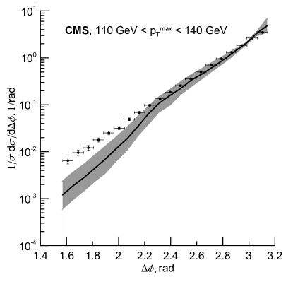
The CMS measurements CMS2 of $F(\Delta\phi)$ distributions for the two most energetic jets are shown in Fig. 1. A comparison of the LO parton Reggeization approach predictions with the data demonstrates a nice agreement in the region of $\Delta\varphi\geq 3\pi/4$. As $\Delta\varphi$ decreases from $3\pi/4$ to $\pi/2$, the theoretical expectations tend to underestimate data more and more, up to a factor of 5 at the $80<p_{T}^{max}<110$ GeV and a factor 2 at the $200<p_{T}^{max}<300$ GeV. This difference follows from our theoretical approximation: we take into account only two-jet production subprocesses in the QMRK, like the $RR\to gg$. However, at $\Delta\varphi\simeq\pi/2$, the contribution of three-jet production subprocess should be important. One can find, the difference becomes smaller with the growing of $p_{T}^{max}$, because the situation when transverse momentum of leading jet is compensated by the one energetic jet in opposite direction is more probable than the such compensation by two or more jets.

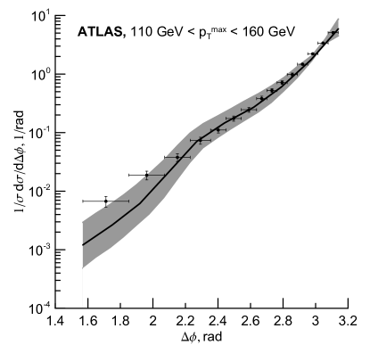
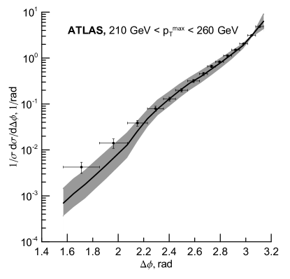
Our observations are confirmed in Fig. 2, where the data from the ATLAS Collaboration ATLAS2 are compared with theoretical predictions. We see that the disagreements between our predictions and ATLAS data are smaller than in the case of CMS data. This fact can be explained by the difference of the choice of low-$p_{T}$ cut for both Collaborations: CMS measurements have been performed for jet production with $p_{T}>30$ GeV, and ATLAS measurements – with $p_{T}>110$ GeV.

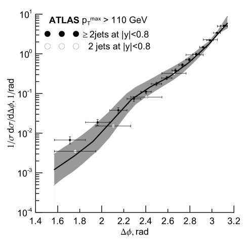
Certainly, the precise comparison of theoretical predictions in the LO parton Reggeization approach should be made when we separate only the two-jet production in the central rapidity region. In fact, the data include a multijet production contribution. The ATLAS Collaboration presents the $\Delta\varphi-$distributions for different numbers of final-state jets (see Fig. 1 in Ref. ATLAS2 ). Using these data, we can extract $F(\Delta\varphi)$ for two-jet production only, as a difference between number of events: $n(2)=n(\geq 2)-n(\geq 3)$ or $\sigma(2)F(\Delta\varphi,2)=\sigma(\geq 2)F(\Delta\varphi,\geq 2)-\sigma(\geq 3)F(\Delta\varphi,\geq 3)$. The original ATLAS data for $F(\Delta\varphi,\geq 2)$ and extracted data for $F(\Delta\varphi,2)$ are shown in Fig. 3 for the kinematic domain of $p_{T}^{max}>100$ GeV and $|y|<0.8$. As we see, the theoretical prediction nicely agrees with data for $F(\Delta\varphi,2)$ distribution. So, if the last one would be extracted for different regions of $p_{T}^{max}$, we can make a more precise comparison of our predictions with experimental data.

Summarizing the results of the present analysis for dijet production at the LHC and our previous study of $b\bar{b}-$pair production at the Tevatron and LHC bbTEV ; bbLHC , we find a strong difference of theoretical interpretation of azimuthal decorrelation between leading and subleading jets, in the collinear parton model and in the parton Reggeization approach. In the first case, an azimuthal decorrelation at different values of $\Delta\varphi$ is provided by hard $2\to 3$ ($3\pi/4<\Delta\varphi<\pi$), $2\to 4$ ($\pi/2<\Delta\varphi<3\pi/4$) partonic subprocesses, correspondingly. The explanation of data in the region of $\Delta\varphi<\pi/2$ in the framework of collinear parton model becomes possible only because of initial-state radiation and hadronization effects, and an agreement of theory expectations and data is achieved using MC generators only.

Oppositely, in the parton Reggeization approach, the azimuthal decorrelation is explained by the coherent parton emission during the QCD evolution, which is described by the transverse-momentum-dependent PDFs of Reggeized partons. Already in the LO approximation, at the level of $2\to 2$ subprocesses with Reggeized partons, we can account the main part of decorrelation effect in dijet production, and we obtain a full description of data in $b\bar{b}$ pair production.

IV Conclusions

This good description of dijet azimuthal decorrelations is achieved in the LO parton Reggeization approach, without any ad hoc adjustments of input parameters. By contrast, in the collinear parton model, such a degree of agreement calls for NLO and NNLO corrections and complementary initial-state radiation effects and ad hoc nonperturbative transverse momenta of partons. In conclusion, the parton Reggeization approach has once again proven to be a powerful tool for the theoretical description of QCD processes induced by Reggeized partons in the high-energy limit. As it was shown by recent studies NLOPRA , the one-loop calculations in this formalism lead the results for the NLO effective vertices, consistent with the earlier calculations based on unitarity relations oldNLOPRA . These results open a possibility to extend the calculations of hard processes in the parton Reggeization approach to the complete NLO level.

Figure 1: Normalized $F(\Delta\phi)$ distributions in several $p_{T}^{max}$ regions at the $\sqrt{S}=7$ TeV, $|y|<1.1$ and $p_{T}>30$ GeV. The data are from the CMS Collaboration CMS2 . The curve corresponds to LO parton Reggeization approach.

Figure 2: Normalized $F(\Delta\phi)$ distributions in several $p_{T}^{max}$ regions at the $\sqrt{S}=7$ TeV, $|y|<0.8$ and $p_{T}>100$ GeV. The data are from the ATLAS Collaboration ATLAS2 . The curve corresponds to LO parton Reggeization approach.

Figure 3: Normalized $F(\Delta\phi)$ distribution for 2 (open circles) and $\geq 2$ (black circles) jets with $p_{T}>100$ GeV, $|y|<0.8$, $p_{T}^{max}>110$ GeV and $\sqrt{S}=7$ TeV. The data are from the ATLAS Collaboration ATLAS2 . The curve corresponds to LO parton Reggeization approach.

Appendix

1. $RR\to gg$

$$A = \frac{18}{a_{1}a_{2}b_{1}b_{2}s^{2}t^{2}u^{2}t_{1}t_{2}},$$

$$W_{0} = x_{1}x_{2}s^{2}tut_{1}t_{2}\bigl{(}x_{1}x_{2}(tu+t_{1}t_{2})+(a_{1}b_{2}+a_{2}b_{1})tu\bigr{)},$$

$$W_{1} = x_{1}x_{2}st_{1}t_{2}\biggl{[}t^{2}u\biggl{(}a_{1}b_{2}(a_{2}b_{2}+a_{1}x_{2})(t_{1}+t_{2})-a_{2}b_{1}(a_{1}b_{1}t_{1}+a_{2}b_{2}t_{2})+$$

$$+ \bigl{(}x_{2}(a_{1}^{2}b_{2}+a_{2}^{2}b_{1})+a_{1}a_{2}(b_{1}-b_{2})^{2}\bigr{)}u+x_{1}x_{2}a_{1}b_{2}t\biggr{)}\biggr{]}+\biggl{[}a_{1}\leftrightarrow a_{2},b_{1}\leftrightarrow b_{2},t\leftrightarrow u\biggr{]},$$

$$W_{2} = a_{1}a_{2}b_{1}b_{2}tu\biggl{(}x_{1}^{2}x_{2}^{2}\bigl{[}2(t_{1}+t_{2})\bigl{(}t^{2}u+t_{1}t_{2}(s+u-t)\bigr{)}+tu\bigl{(}(t_{1}-t_{2})^{2}+t(u+2t)\bigr{)}\bigr{]}+$$

$$+ x_{1}x_{2}tt_{1}t_{2}\bigl{(}4(x_{1}b_{1}+x_{2}a_{2})(s+u)-(a_{1}b_{1}+a_{2}b_{2})u\bigr{)}+$$

$$+ tu\bigl{(}x_{1}^{2}b_{2}(2x_{2}t-b_{1}t_{1})t_{1}+x_{2}^{2}a_{1}(2x_{1}t-a_{2}t_{2})t_{2}\bigr{)}\biggr{)}+\biggl{(}a_{1}\leftrightarrow a_{2},b_{1}\leftrightarrow b_{2},t\leftrightarrow u\biggr{)},$$

$$W_{3} = x_{1}x_{2}a_{1}a_{2}b_{1}b_{2}\biggl{[}t^{2}u\biggl{(}2a_{1}b_{2}\bigl{(}x_{1}x_{2}(t_{1}+t_{2})(2t-u-s)-(x_{1}b_{2}t_{1}+x_{2}a_{1}t_{2})(u+s)\bigr{)}+$$

$$+ \bigl{[}x_{1}t_{1}\bigl{(}2(a_{1}b_{2}^{2}+a_{2}b_{1}^{2})+3x_{1}b_{1}b_{2}\bigr{)}+x_{2}t_{2}\bigl{(}2(a_{1}^{2}b_{2}+a_{2}^{2}b_{1}\bigr{)}+3a_{1}a_{2}x_{2})\bigr{]}u+$$

$$+ 4x_{1}x_{2}t\bigl{(}(a_{1}b_{2}+a_{2}b_{1})u+a_{1}b_{2}t\bigr{)}\biggr{)}\biggr{]}+\biggl{[}a_{1}\leftrightarrow a_{2},b_{1}\leftrightarrow b_{2},t\leftrightarrow u\biggr{]},$$

$$W_{4} = x_{1}^{2}x_{2}^{2}a_{1}a_{2}b_{1}b_{2}\biggl{[}t\biggl{(}a_{1}a_{2}b_{1}b_{2}u(t_{1}+t_{2})(t-u-s)+(a_{1}b_{2}+a_{2}b_{1})^{2}tu^{2}-$$ (35)

$$- 2a_{1}b_{2}t(s+u)(2a_{2}b_{1}u-a_{1}b_{2}s)\biggr{)}\biggr{]}+\biggl{[}a_{1}\leftrightarrow a_{2},b_{1}\leftrightarrow b_{2},t\leftrightarrow u\biggr{]}.$$

2. $RR\to q\bar{q}$

$$A = \frac{S}{3s^{2}t^{2}u^{2}t_{1}t_{2}},$$

$$W_{0} = 18x_{1}x_{2}st^{2}u^{2}t_{1}t_{2},$$

$$W_{1} = tu\biggl{(}-18tu\bigl{(}(x_{1}b_{1}t_{1}-a_{1}x_{2}t_{2})+x_{1}x_{2}(u+t_{2})\bigr{)}\bigl{(}(x_{1}b_{1}t_{1}-a_{1}x_{2}t_{2})-x_{1}x_{2}(t+t_{1})\bigr{)}+$$

$$+ x_{1}x_{2}s\bigl{[}9\bigl{(}(t-u)(a_{1}b_{2}-a_{2}b_{1})t_{1}t_{2}-x_{1}x_{2}stu\bigr{)}-x_{1}x_{2}s(t_{1}t_{2}-tu)\bigr{]}\biggr{)},$$

$$W_{2} = x_{1}x_{2}tu\bigl{[}9\bigl{(}2(x_{1}b_{1}t_{1}-x_{2}a_{1}t_{2})-x_{1}x_{2}(t+t_{1}-u-t_{2})\bigr{)}\times$$

$$\times \bigl{(}2(a_{2}b_{1}-a_{1}b_{2})tu-(a_{1}b_{2}t-a_{2}b_{1}u)s\bigr{)}-7x_{1}x_{2}s^{2}(a_{2}b_{1}u+a_{1}b_{2}t)\bigr{]},$$

$$W_{3} = -x_{1}^{2}x_{2}^{2}\bigl{[}18tu(a_{2}b_{1}-a_{1}b_{2})\bigl{(}(a_{2}b_{1}-a_{1}b_{2})tu+(a_{2}b_{1}u-a_{1}b_{2}t)s\bigr{)}+$$

$$+ 2s^{2}(4a_{2}^{2}b_{1}^{2}u^{2}+4a_{1}^{2}b_{2}^{2}t^{2}-a_{1}a_{2}b_{1}b_{2}tu)\bigr{]},$$

$$W_{4} = 0.$$ (36)

3. $QR\to qg$

$$A = -\frac{8x_{1}}{9a_{2}b_{1}b_{2}st^{2}u^{2}t_{2}},$$

$$W_{0} = -9x_{2}t_{2}stu\bigl{(}x_{2}t_{1}t_{2}+(x_{2}+b_{2})tu\bigr{)},$$

$$W_{1} = tu\biggl{(}-a_{2}b_{1}b_{2}tu\bigl{[}8\bigl{(}b_{1}(s+t)-b_{2}u\bigr{)}+x_{2}s\bigr{]}+$$

$$+ \bigl{[}9x_{2}^{2}\bigl{(}a_{2}(b_{1}-b_{2})s^{2}+(a_{2}b_{1}+a_{1}b_{2})st-a_{1}b_{2}tu\bigr{)}+$$

$$+ 9x_{2}a_{2}u\bigl{(}(b_{1}^{2}-2b_{1}b_{2}-b_{2}^{2})s-b_{1}b_{2}u\bigr{)}+$$

$$+ x_{2}a_{2}b_{1}t\bigl{(}(b_{1}-b_{2})s+b_{1}t\bigr{)}+2a_{2}b_{1}tu(b_{1}^{2}+b_{1}b_{2}+4b_{2}^{2})\bigr{]}t_{2}+$$

$$+ x_{2}\bigl{(}(a_{2}b_{1}t+9a_{2}x_{2}s)(b_{1}-b_{2})+9b_{1}b_{2}u(a_{1}-a_{2})\bigr{)}t_{2}^{2}\biggr{)},$$

$$W_{2} = a_{2}b_{1}b_{2}x_{2}tu\biggl{(}9\bigl{(}a_{1}t(x_{2}s+b_{2}u)-a_{2}u(x_{2}s-b_{2}u)-2a_{2}b_{1}u(t+s)\bigr{)}+$$

$$+ b_{1}t(a_{1}t+a_{2}u)-2a_{1}b_{2}t(s+u)+$$

$$+ \biggl{[}9\bigl{(}x_{1}x_{2}(s+u)+2a_{1}b_{1}u+x_{2}a_{1}(s-3u)\bigr{)}+(b_{1}x_{1}-2a_{1}b_{2})t\bigr{]}t_{2}\biggr{)},$$

$$W_{3} = a_{2}b_{1}b_{2}x_{2}^{2}\biggl{(}9\bigl{[}s\bigl{(}a_{1}^{2}b_{2}t^{2}-2a_{2}^{2}b_{1}u^{2}+a_{1}a_{2}ut(b_{1}-b_{2})\bigr{)}+a_{2}tu^{2}(a_{1}b_{2}-a_{2}b_{1})\bigr{]}-$$

$$- a_{1}t^{2}\bigl{(}u(a_{1}b_{2}-a_{2}b_{1})+a_{1}b_{2}s\bigr{)}\biggr{)},$$

$$W_{4} = 0.$$ (37)

4. $QQ\to qq$

$$A = \frac{64x_{1}x_{2}}{27a_{1}a_{2}b_{1}b_{2}t^{2}u^{2}S},$$

$$W_{0} = -stut_{1}t_{2},$$

$$W_{1} = t^{2}u^{2}\bigl{[}6(a_{1}b_{2}+a_{2}b_{1})-a_{1}b_{1}-a_{2}b_{2}\bigr{]}+stu(a_{1}b_{2}t+a_{2}b_{1}u)-$$

$$- tu\bigl{[}t_{1}(a_{1}b_{1}t+a_{2}b_{2}u)+t_{2}(a_{1}b_{1}u+a_{2}b_{2}t)+t_{1}t_{2}(a_{1}-a_{2})(b_{1}-b_{2})\bigr{]},$$

$$W_{2} = -tu\bigl{[}x_{2}^{2}a_{1}a_{2}t_{1}+x_{1}^{2}b_{1}b_{2}t_{2}+a_{1}b_{2}t(a_{1}b_{1}+x_{1}b_{2}-5a_{2}b_{1})+a_{2}b_{1}u(a_{1}b_{1}+x_{2}a_{2}-5a_{1}b_{2})\bigr{]},$$

$$W_{3} = 3a_{1}a_{2}b_{1}b_{2}(a_{1}b_{2}t^{2}+a_{2}b_{1}u^{2}),$$

$$W_{4} = 0.$$ (38)

5. $QQ^{\prime}\to qq^{\prime}$

$$A=\frac{64x_{1}x_{2}}{9a_{2}b_{1}t^{2}},\qquad W_{0}=2t^{2},\quad W_{1}=2a_{2}b_{1}t,\quad W_{2}=a_{2}^{2}b_{1}^{2},\quad W_{3}=0,\quad W_{4}=0.$$ (39)

6. $Q\bar{Q}\to q\bar{q}$

$$A = \frac{64}{27x_{1}x_{2}a_{2}b_{1}s^{2}t^{2}},$$

$$W_{0} = x_{1}x_{2}st\bigl{[}t_{1}t(3a_{2}b_{1}-x_{1}b_{2})+t_{2}t(3a_{2}b_{1}-x_{2}a_{1})+t_{1}t_{2}(x_{2}a_{2}-x_{1}b_{2})-x_{1}x_{2}t^{2}+$$

$$+ st\bigl{(}6(a_{1}b_{1}+a_{2}b_{2})+5(2a_{2}b_{1}+a_{1}b_{2})\bigr{)}\bigr{]},$$

$$W_{1} = t\bigl{[}t_{1}x_{1}a_{2}b_{2}\bigl{(}6b_{1}t(a_{2}b_{1}-a_{1}b_{2})-x_{2}s(x_{1}b_{1}+a_{2}b_{1}-a_{1}b_{2})\bigr{)}+$$

$$+ t_{2}x_{2}a_{1}b_{1}\bigl{(}6a_{2}t(a_{2}b_{1}-a_{1}b_{2})-x_{1}s(x_{2}a_{2}+a_{2}b_{1}-a_{1}b_{2})\bigr{)}+$$

$$+ 6x_{1}x_{2}a_{2}b_{1}(a_{2}b_{1}-a_{1}b_{2})t^{2}+x_{1}x_{2}a_{2}b_{1}s^{2}(a_{2}b_{1}-a_{1}b_{2}+6x_{1}x_{2})+$$

$$+ x_{1}x_{2}st\bigl{(}(a_{1}b_{2}-a_{2}b_{1})^{2}+a_{1}b_{2}(a_{1}b_{1}+a_{2}b_{2})-2a_{2}b_{1}(2a_{2}b_{1}+x_{1}b_{2}+x_{2}a_{1})\bigr{)}\bigr{]},$$

$$W_{2} = x_{1}x_{2}a_{2}b_{1}\bigl{(}{6t^{2}}(a_{2}b_{1}-a_{1}b_{2})^{2}+3x_{1}x_{2}a_{2}b_{1}s^{2}+st(x_{1}b_{1}+x_{2}a_{2})(a_{1}b_{2}-a_{2}b_{1})\bigr{)},$$

$$W_{3} = W_{4}=0.$$ (40)

7. $Q\bar{Q}\to q^{\prime}\bar{q}^{\prime}$

$$A = \frac{64}{9x_{1}x_{2}s^{2}},$$

$$W_{0} = -x_{1}x_{2}s(t+u),$$

$$W_{1} = 2\bigl{(}a_{1}^{2}b_{1}b_{2}(t_{1}+u)+a_{1}^{2}b_{2}^{2}u+a_{1}a_{2}b_{1}^{2}(t+t_{2})+a_{1}a_{2}b_{1}b_{2}(t_{1}+t_{2}-s)+$$

$$+ a_{1}a_{2}b_{2}^{2}(t_{2}+u)+a_{2}^{2}b_{1}^{2}t+a_{2}^{2}b_{1}b_{2}(t_{1}+t)\bigr{)},$$

$$W_{2} = 2x_{1}x_{2}(a_{2}b_{1}-a_{1}b_{2})^{2},$$

$$W_{3} = W_{4}=0.$$ (41)

8. $Q\bar{Q}\to gg$

$$A = \frac{1}{27x_{1}x_{2}Sa_{1}a_{2}b_{1}b_{2}s^{2}t^{2}u^{2}},$$

$$W_{0} = 2x_{1}x_{2}s^{2}tu\bigl{[}\bigl{(}x_{1}x_{2}-9(a_{1}b_{2}+a_{2}b_{1})\bigr{)}(t+u)tu-x_{1}x_{2}t_{1}t_{2}(t_{1}+t_{2})\bigr{]}+\bigl{[}a_{1}\leftrightarrow a_{2},b_{1}\leftrightarrow b_{2},t\leftrightarrow u\bigr{]},$$

$$W_{1} = -2x_{1}x_{2}stu\biggl{(}x_{1}x_{2}(a_{1}-a_{2})(b_{1}-b_{2})(t_{1}+t_{2})t_{1}t_{2}+2t\bigl{[}x_{1}x_{2}(x_{1}b_{2}t_{2}^{2}+x_{2}a_{1}t_{1}^{2})+$$

$$+ t_{1}t_{2}\bigl{(}(x_{1}x_{2}+x_{1}b_{2}+x_{2}a_{1})(a_{1}b_{1}+a_{2}b_{2})+(8a_{2}b_{1}-a_{1}b_{2})(a_{2}b_{1}-a_{1}b_{2})\bigr{)}\bigr{]}+$$

$$+ x_{1}x_{2}\bigl{(}2x_{1}x_{2}-17(a_{1}b_{2}+a_{2}b_{1})\bigr{)}(t_{1}+t_{2})tu+2\bigl{(}x_{1}^{2}(x_{2}+b_{1})(b_{2}-8b_{1})+$$

$$+ x_{2}^{2}a_{1}(a_{2}-8a_{1})+a_{1}b_{1}(25x_{1}x_{2}-72a_{2}b_{2})\bigr{)}t^{2}u+2t^{2}(x_{1}x_{2}-9a_{2}b_{1})(x_{1}b_{2}t_{2}+x_{2}a_{1}t_{1})\biggr{)}+$$

$$+ \biggl{(}a_{1}\leftrightarrow a_{2},b_{1}\leftrightarrow b_{2},t\leftrightarrow u\biggr{)},$$

$$W_{2} = \biggl{[}-2tu\biggl{(}-x_{1}^{2}x_{2}^{4}a_{1}a_{2}(t_{1}+t_{2})^{2}t_{1}+2x_{1}x_{2}a_{1}tt_{1}(t_{1}+t_{2})\bigl{[}x_{2}^{2}\bigl{(}9a_{1}^{2}b_{1}-x_{1}(x_{1}x_{2}+a_{1}b_{2})\bigr{)}+$$

$$+ x_{1}(8b_{1}-b_{2})\bigl{(}x_{2}^{2}(a_{2}-a_{1})+a_{2}b_{2}^{2}\bigr{)}\bigr{]}+$$

$$+ x_{1}tut_{1}\bigl{(}36x_{1}a_{1}a_{2}b_{2}^{3}(b_{2}-2x_{2})+5a_{1}a_{2}x_{1}x_{2}^{2}b_{2}^{2}-x_{2}^{4}a_{2}(x_{1}+a_{1})(2a_{1}-7a_{2})+$$

$$+ 9x_{2}^{2}b_{2}(x_{1}^{3}b_{2}-2x_{2}a_{1}^{3}+4x_{1}^{2}x_{2}a_{1})-4x_{1}x_{2}^{3}b_{2}(a_{1}^{2}+4x_{1}^{2})\bigr{)}+2x_{1}x_{2}a_{1}t^{2}t_{1}\times$$

$$\times \bigl{[}9a_{2}\bigl{(}b_{2}^{2}(3x_{1}b_{1}-2x_{2}a_{1})-x_{2}^{2}b_{2}(x_{1}-3a_{1})+x_{2}^{3}a_{2}\bigr{)}-2x_{1}x_{2}b_{2}(a_{1}x_{2}+a_{2}b_{2})-x_{1}x_{2}^{3}a_{2}\bigr{]}+$$

$$+ x_{1}x_{2}t^{2}u\bigl{(}a_{1}^{3}b_{2}(7b_{2}^{2}+10b_{1}b_{2}-4b_{1}^{2})+a_{1}^{2}a_{2}b_{1}(39b_{2}^{2}+30b_{1}b_{2}-2b_{1}^{2})+$$

$$+ 14a_{1}a_{2}^{2}b_{1}^{2}(x_{2}+2b_{2})+8a_{2}^{3}b_{1}^{3}\bigr{)}+x_{1}x_{2}a_{1}b_{2}t^{3}\bigl{(}18a_{2}b_{1}(a_{1}x_{2}+x_{1}b_{2})-x_{1}x_{2}(a_{1}b_{1}+x_{1}b_{2})\bigr{)}\biggr{)}+$$

$$+ \biggl{(}a_{1}\leftrightarrow b_{2},a_{2}\leftrightarrow b_{1},x_{1}\leftrightarrow x_{2},t_{1}\leftrightarrow t_{2}\biggr{)}\biggr{]}+\biggl{[}a_{1}\leftrightarrow a_{2},b_{1}\leftrightarrow b_{2},t\leftrightarrow u\biggr{]},$$

$$W_{3} = -4x_{1}x_{2}a_{1}a_{2}b_{1}b_{2}\biggl{(}t^{2}\bigl{[}8x_{1}x_{2}a_{1}b_{2}(s+u)^{2}-u(s+u)\bigl{(}(9a_{2}b_{1}+7a_{1}b_{2})(a_{1}b_{1}+a_{2}b_{2})+$$

$$+ 2a_{1}b_{2}(17a_{2}b_{1}-a_{1}b_{2})\bigr{)}+2a_{1}u^{2}\bigl{(}4b_{1}(a_{1}b_{2}+a_{2}b_{1})+b_{2}(13a_{1}b_{2}-5a_{2}b_{1})\bigr{)}\bigr{]}\biggr{)}+$$

$$+ \biggl{(}a_{1}\leftrightarrow a_{2},b_{1}\leftrightarrow b_{2},t\leftrightarrow u\biggr{)},$$

$$W_{4} = 0.$$ (42)

Erratum:
M.A. Nefedov, V.A. Saleev, A.V. Shipilova, Dijet azimuthal decorrelations at the LHC in the parton Reggeization approach, Phys. Rev. D87, 094030 (2013)

The following corrections should be made to the expressions for squared matrix elements of $2\to 2$ processes in parton Reggeization approach, which has been published in the Appendix of Phys. Rev. D87, 094030 (2013).

1. For the squared matrix element 3, the factor $a_{1}$ has been lost in the last term of $W_{3}$ in the published version. The correct term has a form: $a_{1}t^{2}\bigl{(}u(a_{1}b_{2}-a_{2}b_{1})+a_{1}b_{2}s\bigr{)}$.

2. In the squared matrix element 4 the whole term $(\pi^{2}\alpha_{s}^{2})\cdot\dfrac{64x_{1}x_{2}}{27a_{1}a_{2}b_{1}b_{2}t^{2}u^{2}}\cdot(-stut_{1}t_{2}/S)$ should be added to the squared amplitude, presented in the journal. Restoration of the structure of decomposition of the squared amplitude in powers of $S$ requires the change of $A$ and $W_{i}$ coefficients.

3. While interpreting the published expression for the squared matrix element 8, the reader should note, that the replacements $a_{1}\leftrightarrow b_{2}$ and $a_{2}\leftrightarrow b_{1}$ in the square braces of $W_{2}$ should be accompanied by the replacement $x_{1}\leftrightarrow x_{2}$, since $x_{1}=a_{1}+a_{2}$ and $x_{2}=b_{1}+b_{2}$.

The given misprints in the expressions appeared only at the stage of preparation to the publication. The equivalent but less compact form of the squared amplitudes has been used in the numerical calculations, therefore, the published numerical results are unaffected.

Recently [K. Kutak, R. Maciula, M. Serino, A. Szczurek, A. van Hameren, ”Four-jet production in single- and double-parton scattering within high-energy factorization”, JHEP 1604 (2016) 175], it has been performed a comparison of the cross sections for dijet production obtained both with the QCD amplitudes from the parton Reggeization approach and those from the AVHLIB [A. van Hameren, ”BCFW recursion for off-shell gluons,” JHEP, 07(2014), 138, 1404. 7818; A. van Hameren and M. Serino, ”BCFW recursion for TMD parton scattering,” JHEP, 07(2015), 010, 1504.00315]. The perfect agreement has been found. The consistency between amplitudes computed in different approaches is a non-trivial check of the methods employed.

The current version of the Appendix contains the corrected expressions for the coefficients of the decomposition of the squared amplitudes.

We wish to thank Krzysztof Kutak, Rafal Maciula, Mirko Serino, Antoni Szczurek, and Andreas van Hameren for useful discussion of the obtained results on analytic formula for matrix elements.

References

• (1) B.L. Ioffe, V.S. Fadin and L.N. Lipatov, Quantum chromodynamics. Perturbative and nonperturbative aspects. Cambridge University Press, 2010, Cambridge, UK; D. Green, High 𝒑𝑻subscript𝒑𝑻p_{T} physics at hadron colliders. Cambridge University Press, 2005, Cambridge, UK.
• (2) CMS Collaboration, V. Khachatryan at al., Phys. Rev. Lett. 106, 122003 (2011).
• (3) ATLAS Collaboration, G. Aad et al., Phys. Rev. Lett. 106, 172002 (2011).
• (4) B. A. Kniehl, V. A. Saleev, A. V. Shipilova, E. V. Yatsenko, Phys. Rev.  D84 , 074017 (2011).
• (5) V. S. Fadin and L. N. Lipatov, Nucl. Phys.  B406, 259 (1993); B477, 767 (1996).
• (6) V. S. Fadin and V. E. Sherman, JETP Lett. 23, 599 (1976); JETP 45, 861 (1977).
• (7) L. N. Lipatov, Nucl. Phys.  B452, 369 (1995).
• (8) L. N. Lipatov and M. I. Vyazovsky, Nucl. Phys.  B597, 399 (2001).
• (9) V. A. Saleev, Phys. Rev.  D 78, 034033 (2008).
• (10) V. A. Saleev, Phys. Rev.  D 78, 114031 (2008).
• (11) M.A. Nefedov, N.N. Nikolaev, and V.A. Saleev, Phys. Rev. D 87, 014022 (2013).
• (12) B. A. Kniehl, V. A. Saleev, and A. V. Shipilova Phys. Rev. D 81, 094010 (2010).
• (13) V.A. Saleev, A.V. Shipilova, Phys. Rev. D86, 034032 (2012).
• (14) L. N. Lipatov, Sov. J. Nucl. Phys.  23, 338 (1976) [Yad. Fiz.  23, 642 (1976)]; E. A. Kuraev, L. N. Lipatov, and V. S. Fadin, Sov. Phys. JETP 44, 443 (1976) [Zh. Eksp. Teor. Fiz.  71, 840 (1976)]; Sov. Phys. JETP 45, 199 (1977) [Zh. Eksp. Teor. Fiz.  72, 377 (1977)]; I. I. Balitsky and L. N. Lipatov, Sov. J. Nucl. Phys.  28, 822 (1978) [Yad. Fiz.  28, 1597 (1978)]; Sov. Phys. JETP 63, 904 (1986) [Zh. Eksp. Teor. Fiz.  90, 1536 (1986)].
• (15) V. N. Gribov and L. N. Lipatov, Sov. J. Nucl. Phys. 15, 438 (1972) [Yad. Fiz. 15, 781 (1972)]; Yu. L. Dokshitzer, Sov. Phys. JETP 46, 641 (1977) [Zh. Eksp. Teor. Fiz. 73, 1216 (1977)]; G. Altarelli and G. Parisi, Nucl. Phys. B126, 298 (1977).
• (16) E. N. Antonov, L. N. Lipatov, E. A. Kuraev, and I. O. Cherednikov, Nucl. Phys.  B721, 111 (2005).
• (17) M. A. Kimber, A. D. Martin, and M. G. Ryskin, Eur. Phys. J.  C 12, 655 (2000); Phys. Rev.  D 63, 114027 (2001); G. Watt, A. D. Martin, and M. G. Ryskin, Eur. Phys. J.  C 31, 73 (2003).
• (18) A. D. Martin, W. J. Stirling, R. S. Thorne, Phys. Lett.  B636 259 (2006).
• (19) V.A. Saleev, Phys. Rev. D 80, 114016 (2009).
• (20) Z. Nagy, Phys. Rev. Lett. 88, 122003 (2002).
• (21) T. Sjostrand, S. Mrenna, and P. Skands, Comput. Phys. Communn. 178, 852 (2008).
• (22) J. Alwall et al., J. High Energy Phys. 09, 028 (2007)
• (23) M. Hentschinski, A. S. Vera, Phys. Rev. D85, 056006 (2012), G. Chachamis, M. Hentschinski, J. D. Madrigal, A. S. Vera, [arXiv: 1212.4992 [hep-ph]] (2012).
• (24) V. Fadin, R. Fiore, A. Quartarolo, Phys. Rev. D50, 2265 (1994), Phys. Rev. D50, 5893 (1994), V. S. Fadin, R. Fiore, M. I. Kotsky, A. Papa, Phys. Rev. D61, 094005 (2000) V. S. Fadin, R. Fiore, A. Papa, Phys. Rev. D63, 034001 (2000).
Refer to caption
Figure 1: Normalized 𝑭(𝚫ϕ)𝑭𝚫bold-italic-ϕF(\Delta\phi) distributions in several 𝒑𝑻𝒎𝒂𝒙superscriptsubscript𝒑𝑻𝒎𝒂𝒙p_{T}^{max} regions at the 𝑺=𝟕𝑺7\sqrt{S}=7 TeV, |𝒚|<1.1𝒚1.1|y|<1.1 and 𝒑𝑻>𝟑𝟎subscript𝒑𝑻30p_{T}>30 GeV. The data are from the CMS Collaboration CMS2 . The curve corresponds to LO parton Reggeization approach.
Figure 2: Normalized 𝑭(𝚫ϕ)𝑭𝚫bold-italic-ϕF(\Delta\phi) distributions in several 𝒑𝑻𝒎𝒂𝒙superscriptsubscript𝒑𝑻𝒎𝒂𝒙p_{T}^{max} regions at the 𝑺=𝟕𝑺7\sqrt{S}=7 TeV, |𝒚|<0.8𝒚0.8|y|<0.8 and 𝒑𝑻>𝟏𝟎𝟎subscript𝒑𝑻100p_{T}>100 GeV. The data are from the ATLAS Collaboration ATLAS2 . The curve corresponds to LO parton Reggeization approach.
Figure 3: Normalized 𝑭(𝚫ϕ)𝑭𝚫bold-italic-ϕF(\Delta\phi) distribution for 2 (open circles) and 𝟐absent2\geq 2 (black circles) jets with 𝒑𝑻>𝟏𝟎𝟎subscript𝒑𝑻100p_{T}>100 GeV, |𝒚|<0.8𝒚0.8|y|<0.8, 𝒑𝑻𝒎𝒂𝒙>𝟏𝟏𝟎superscriptsubscript𝒑𝑻𝒎𝒂𝒙110p_{T}^{max}>110 GeV and 𝑺=𝟕𝑺7\sqrt{S}=7 TeV. The data are from the ATLAS Collaboration ATLAS2 . The curve corresponds to LO parton Reggeization approach.
Appendix
1. 𝑹𝑹𝒈𝒈bold-→𝑹𝑹𝒈𝒈RR\to gg
𝑨𝑨\displaystyle A =\displaystyle= 𝟏𝟖𝒂𝟏𝒂𝟐𝒃𝟏𝒃𝟐𝒔𝟐𝒕𝟐𝒖𝟐𝒕𝟏𝒕𝟐,18subscript𝒂1subscript𝒂2subscript𝒃1subscript𝒃2superscript𝒔2superscript𝒕2superscript𝒖2subscript𝒕1subscript𝒕2\displaystyle\frac{18}{a_{1}a_{2}b_{1}b_{2}s^{2}t^{2}u^{2}t_{1}t_{2}},
𝑾𝟎subscript𝑾0\displaystyle W_{0} =\displaystyle= 𝒙𝟏𝒙𝟐𝒔𝟐𝒕𝒖𝒕𝟏𝒕𝟐(𝒙𝟏𝒙𝟐(𝒕𝒖+𝒕𝟏𝒕𝟐)+(𝒂𝟏𝒃𝟐+𝒂𝟐𝒃𝟏)𝒕𝒖),subscript𝒙1subscript𝒙2superscript𝒔2𝒕𝒖subscript𝒕1subscript𝒕2subscript𝒙1subscript𝒙2𝒕𝒖subscript𝒕1subscript𝒕2subscript𝒂1subscript𝒃2subscript𝒂2subscript𝒃1𝒕𝒖\displaystyle x_{1}x_{2}s^{2}tut_{1}t_{2}\bigl{(}x_{1}x_{2}(tu+t_{1}t_{2})+(a_{1}b_{2}+a_{2}b_{1})tu\bigr{)},
𝑾𝟏subscript𝑾1\displaystyle W_{1} =\displaystyle= 𝒙𝟏𝒙𝟐𝒔𝒕𝟏𝒕𝟐[𝒕𝟐𝒖(𝒂𝟏𝒃𝟐(𝒂𝟐𝒃𝟐+𝒂𝟏𝒙𝟐)(𝒕𝟏+𝒕𝟐)𝒂𝟐𝒃𝟏(𝒂𝟏𝒃𝟏𝒕𝟏+𝒂𝟐𝒃𝟐𝒕𝟐)+\displaystyle x_{1}x_{2}st_{1}t_{2}\biggl{[}t^{2}u\biggl{(}a_{1}b_{2}(a_{2}b_{2}+a_{1}x_{2})(t_{1}+t_{2})-a_{2}b_{1}(a_{1}b_{1}t_{1}+a_{2}b_{2}t_{2})+
+\displaystyle+ (𝒙𝟐(𝒂𝟏𝟐𝒃𝟐+𝒂𝟐𝟐𝒃𝟏)+𝒂𝟏𝒂𝟐(𝒃𝟏𝒃𝟐)𝟐)𝒖+𝒙𝟏𝒙𝟐𝒂𝟏𝒃𝟐𝒕)]+[𝒂𝟏𝒂𝟐,𝒃𝟏𝒃𝟐,𝒕𝒖],\displaystyle\bigl{(}x_{2}(a_{1}^{2}b_{2}+a_{2}^{2}b_{1})+a_{1}a_{2}(b_{1}-b_{2})^{2}\bigr{)}u+x_{1}x_{2}a_{1}b_{2}t\biggr{)}\biggr{]}+\biggl{[}a_{1}\leftrightarrow a_{2},b_{1}\leftrightarrow b_{2},t\leftrightarrow u\biggr{]},
𝑾𝟐subscript𝑾2\displaystyle W_{2} =\displaystyle= 𝒂𝟏𝒂𝟐𝒃𝟏𝒃𝟐𝒕𝒖(𝒙𝟏𝟐𝒙𝟐𝟐[𝟐(𝒕𝟏+𝒕𝟐)(𝒕𝟐𝒖+𝒕𝟏𝒕𝟐(𝒔+𝒖𝒕))+𝒕𝒖((𝒕𝟏𝒕𝟐)𝟐+𝒕(𝒖+𝟐𝒕))]+\displaystyle a_{1}a_{2}b_{1}b_{2}tu\biggl{(}x_{1}^{2}x_{2}^{2}\bigl{[}2(t_{1}+t_{2})\bigl{(}t^{2}u+t_{1}t_{2}(s+u-t)\bigr{)}+tu\bigl{(}(t_{1}-t_{2})^{2}+t(u+2t)\bigr{)}\bigr{]}+
+\displaystyle+ 𝒙𝟏𝒙𝟐𝒕𝒕𝟏𝒕𝟐(𝟒(𝒙𝟏𝒃𝟏+𝒙𝟐𝒂𝟐)(𝒔+𝒖)(𝒂𝟏𝒃𝟏+𝒂𝟐𝒃𝟐)𝒖)+limit-fromsubscript𝒙1subscript𝒙2𝒕subscript𝒕1subscript𝒕24subscript𝒙1subscript𝒃1subscript𝒙2subscript𝒂2𝒔𝒖subscript𝒂1subscript𝒃1subscript𝒂2subscript𝒃2𝒖\displaystyle x_{1}x_{2}tt_{1}t_{2}\bigl{(}4(x_{1}b_{1}+x_{2}a_{2})(s+u)-(a_{1}b_{1}+a_{2}b_{2})u\bigr{)}+
+\displaystyle+ 𝒕𝒖(𝒙𝟏𝟐𝒃𝟐(𝟐𝒙𝟐𝒕𝒃𝟏𝒕𝟏)𝒕𝟏+𝒙𝟐𝟐𝒂𝟏(𝟐𝒙𝟏𝒕𝒂𝟐𝒕𝟐)𝒕𝟐))+(𝒂𝟏𝒂𝟐,𝒃𝟏𝒃𝟐,𝒕𝒖),\displaystyle tu\bigl{(}x_{1}^{2}b_{2}(2x_{2}t-b_{1}t_{1})t_{1}+x_{2}^{2}a_{1}(2x_{1}t-a_{2}t_{2})t_{2}\bigr{)}\biggr{)}+\biggl{(}a_{1}\leftrightarrow a_{2},b_{1}\leftrightarrow b_{2},t\leftrightarrow u\biggr{)},
𝑾𝟑subscript𝑾3\displaystyle W_{3} =\displaystyle= 𝒙𝟏𝒙𝟐𝒂𝟏𝒂𝟐𝒃𝟏𝒃𝟐[𝒕𝟐𝒖(𝟐𝒂𝟏𝒃𝟐(𝒙𝟏𝒙𝟐(𝒕𝟏+𝒕𝟐)(𝟐𝒕𝒖𝒔)(𝒙𝟏𝒃𝟐𝒕𝟏+𝒙𝟐𝒂𝟏𝒕𝟐)(𝒖+𝒔))+\displaystyle x_{1}x_{2}a_{1}a_{2}b_{1}b_{2}\biggl{[}t^{2}u\biggl{(}2a_{1}b_{2}\bigl{(}x_{1}x_{2}(t_{1}+t_{2})(2t-u-s)-(x_{1}b_{2}t_{1}+x_{2}a_{1}t_{2})(u+s)\bigr{)}+
+\displaystyle+ [𝒙𝟏𝒕𝟏(𝟐(𝒂𝟏𝒃𝟐𝟐+𝒂𝟐𝒃𝟏𝟐)+𝟑𝒙𝟏𝒃𝟏𝒃𝟐)+𝒙𝟐𝒕𝟐(𝟐(𝒂𝟏𝟐𝒃𝟐+𝒂𝟐𝟐𝒃𝟏)+𝟑𝒂𝟏𝒂𝟐𝒙𝟐)]𝒖+limit-fromdelimited-[]subscript𝒙1subscript𝒕12subscript𝒂1superscriptsubscript𝒃22subscript𝒂2superscriptsubscript𝒃123subscript𝒙1subscript𝒃1subscript𝒃2subscript𝒙2subscript𝒕22superscriptsubscript𝒂12subscript𝒃2superscriptsubscript𝒂22subscript𝒃13subscript𝒂1subscript𝒂2subscript𝒙2𝒖\displaystyle\bigl{[}x_{1}t_{1}\bigl{(}2(a_{1}b_{2}^{2}+a_{2}b_{1}^{2})+3x_{1}b_{1}b_{2}\bigr{)}+x_{2}t_{2}\bigl{(}2(a_{1}^{2}b_{2}+a_{2}^{2}b_{1}\bigr{)}+3a_{1}a_{2}x_{2})\bigr{]}u+
+\displaystyle+ 𝟒𝒙𝟏𝒙𝟐𝒕((𝒂𝟏𝒃𝟐+𝒂𝟐𝒃𝟏)𝒖+𝒂𝟏𝒃𝟐𝒕))]+[𝒂𝟏𝒂𝟐,𝒃𝟏𝒃𝟐,𝒕𝒖],\displaystyle 4x_{1}x_{2}t\bigl{(}(a_{1}b_{2}+a_{2}b_{1})u+a_{1}b_{2}t\bigr{)}\biggr{)}\biggr{]}+\biggl{[}a_{1}\leftrightarrow a_{2},b_{1}\leftrightarrow b_{2},t\leftrightarrow u\biggr{]},
𝑾𝟒subscript𝑾4\displaystyle W_{4} =\displaystyle= 𝒙𝟏𝟐𝒙𝟐𝟐𝒂𝟏𝒂𝟐𝒃𝟏𝒃𝟐[𝒕(𝒂𝟏𝒂𝟐𝒃𝟏𝒃𝟐𝒖(𝒕𝟏+𝒕𝟐)(𝒕𝒖𝒔)+(𝒂𝟏𝒃𝟐+𝒂𝟐𝒃𝟏)𝟐𝒕𝒖𝟐\displaystyle x_{1}^{2}x_{2}^{2}a_{1}a_{2}b_{1}b_{2}\biggl{[}t\biggl{(}a_{1}a_{2}b_{1}b_{2}u(t_{1}+t_{2})(t-u-s)+(a_{1}b_{2}+a_{2}b_{1})^{2}tu^{2}- (35)
\displaystyle- 𝟐𝒂𝟏𝒃𝟐𝒕(𝒔+𝒖)(𝟐𝒂𝟐𝒃𝟏𝒖𝒂𝟏𝒃𝟐𝒔))]+[𝒂𝟏𝒂𝟐,𝒃𝟏𝒃𝟐,𝒕𝒖].\displaystyle 2a_{1}b_{2}t(s+u)(2a_{2}b_{1}u-a_{1}b_{2}s)\biggr{)}\biggr{]}+\biggl{[}a_{1}\leftrightarrow a_{2},b_{1}\leftrightarrow b_{2},t\leftrightarrow u\biggr{]}.
2. 𝑹𝑹𝒒𝒒¯bold-→𝑹𝑹𝒒bold-¯𝒒RR\to q\bar{q}
𝑨𝑨\displaystyle A =\displaystyle= 𝑺𝟑𝒔𝟐𝒕𝟐𝒖𝟐𝒕𝟏𝒕𝟐,𝑺3superscript𝒔2superscript𝒕2superscript𝒖2subscript𝒕1subscript𝒕2\displaystyle\frac{S}{3s^{2}t^{2}u^{2}t_{1}t_{2}},
𝑾𝟎subscript𝑾0\displaystyle W_{0} =\displaystyle= 𝟏𝟖𝒙𝟏𝒙𝟐𝒔𝒕𝟐𝒖𝟐𝒕𝟏𝒕𝟐,18subscript𝒙1subscript𝒙2𝒔superscript𝒕2superscript𝒖2subscript𝒕1subscript𝒕2\displaystyle 18x_{1}x_{2}st^{2}u^{2}t_{1}t_{2},
𝑾𝟏subscript𝑾1\displaystyle W_{1} =\displaystyle= 𝒕𝒖(𝟏𝟖𝒕𝒖((𝒙𝟏𝒃𝟏𝒕𝟏𝒂𝟏𝒙𝟐𝒕𝟐)+𝒙𝟏𝒙𝟐(𝒖+𝒕𝟐))((𝒙𝟏𝒃𝟏𝒕𝟏𝒂𝟏𝒙𝟐𝒕𝟐)𝒙𝟏𝒙𝟐(𝒕+𝒕𝟏))+\displaystyle tu\biggl{(}-18tu\bigl{(}(x_{1}b_{1}t_{1}-a_{1}x_{2}t_{2})+x_{1}x_{2}(u+t_{2})\bigr{)}\bigl{(}(x_{1}b_{1}t_{1}-a_{1}x_{2}t_{2})-x_{1}x_{2}(t+t_{1})\bigr{)}+
+\displaystyle+ 𝒙𝟏𝒙𝟐𝒔[𝟗((𝒕𝒖)(𝒂𝟏𝒃𝟐𝒂𝟐𝒃𝟏)𝒕𝟏𝒕𝟐𝒙𝟏𝒙𝟐𝒔𝒕𝒖)𝒙𝟏𝒙𝟐𝒔(𝒕𝟏𝒕𝟐𝒕𝒖)]),\displaystyle x_{1}x_{2}s\bigl{[}9\bigl{(}(t-u)(a_{1}b_{2}-a_{2}b_{1})t_{1}t_{2}-x_{1}x_{2}stu\bigr{)}-x_{1}x_{2}s(t_{1}t_{2}-tu)\bigr{]}\biggr{)},
𝑾𝟐subscript𝑾2\displaystyle W_{2} =\displaystyle= 𝒙𝟏𝒙𝟐𝒕𝒖[𝟗(𝟐(𝒙𝟏𝒃𝟏𝒕𝟏𝒙𝟐𝒂𝟏𝒕𝟐)𝒙𝟏𝒙𝟐(𝒕+𝒕𝟏𝒖𝒕𝟐))×\displaystyle x_{1}x_{2}tu\bigl{[}9\bigl{(}2(x_{1}b_{1}t_{1}-x_{2}a_{1}t_{2})-x_{1}x_{2}(t+t_{1}-u-t_{2})\bigr{)}\times
×\displaystyle\times (𝟐(𝒂𝟐𝒃𝟏𝒂𝟏𝒃𝟐)𝒕𝒖(𝒂𝟏𝒃𝟐𝒕𝒂𝟐𝒃𝟏𝒖)𝒔)𝟕𝒙𝟏𝒙𝟐𝒔𝟐(𝒂𝟐𝒃𝟏𝒖+𝒂𝟏𝒃𝟐𝒕)],\displaystyle\bigl{(}2(a_{2}b_{1}-a_{1}b_{2})tu-(a_{1}b_{2}t-a_{2}b_{1}u)s\bigr{)}-7x_{1}x_{2}s^{2}(a_{2}b_{1}u+a_{1}b_{2}t)\bigr{]},
𝑾𝟑subscript𝑾3\displaystyle W_{3} =\displaystyle= 𝒙𝟏𝟐𝒙𝟐𝟐[𝟏𝟖𝒕𝒖(𝒂𝟐𝒃𝟏𝒂𝟏𝒃𝟐)((𝒂𝟐𝒃𝟏𝒂𝟏𝒃𝟐)𝒕𝒖+(𝒂𝟐𝒃𝟏𝒖𝒂𝟏𝒃𝟐𝒕)𝒔)+\displaystyle-x_{1}^{2}x_{2}^{2}\bigl{[}18tu(a_{2}b_{1}-a_{1}b_{2})\bigl{(}(a_{2}b_{1}-a_{1}b_{2})tu+(a_{2}b_{1}u-a_{1}b_{2}t)s\bigr{)}+
+\displaystyle+ 𝟐𝒔𝟐(𝟒𝒂𝟐𝟐𝒃𝟏𝟐𝒖𝟐+𝟒𝒂𝟏𝟐𝒃𝟐𝟐𝒕𝟐𝒂𝟏𝒂𝟐𝒃𝟏𝒃𝟐𝒕𝒖)],\displaystyle 2s^{2}(4a_{2}^{2}b_{1}^{2}u^{2}+4a_{1}^{2}b_{2}^{2}t^{2}-a_{1}a_{2}b_{1}b_{2}tu)\bigr{]},
𝑾𝟒subscript𝑾4\displaystyle W_{4} =\displaystyle= 𝟎.0\displaystyle 0. (36)
3. 𝑸𝑹𝒒𝒈bold-→𝑸𝑹𝒒𝒈QR\to qg
𝑨𝑨\displaystyle A =\displaystyle= 𝟖𝒙𝟏𝟗𝒂𝟐𝒃𝟏𝒃𝟐𝒔𝒕𝟐𝒖𝟐𝒕𝟐,8subscript𝒙19subscript𝒂2subscript𝒃1subscript𝒃2𝒔superscript𝒕2superscript𝒖2subscript𝒕2\displaystyle-\frac{8x_{1}}{9a_{2}b_{1}b_{2}st^{2}u^{2}t_{2}},
𝑾𝟎subscript𝑾0\displaystyle W_{0} =\displaystyle= 𝟗𝒙𝟐𝒕𝟐𝒔𝒕𝒖(𝒙𝟐𝒕𝟏𝒕𝟐+(𝒙𝟐+𝒃𝟐)𝒕𝒖),9subscript𝒙2subscript𝒕2𝒔𝒕𝒖subscript𝒙2subscript𝒕1subscript𝒕2subscript𝒙2subscript𝒃2𝒕𝒖\displaystyle-9x_{2}t_{2}stu\bigl{(}x_{2}t_{1}t_{2}+(x_{2}+b_{2})tu\bigr{)},
𝑾𝟏subscript𝑾1\displaystyle W_{1} =\displaystyle= 𝒕𝒖(𝒂𝟐𝒃𝟏𝒃𝟐𝒕𝒖[𝟖(𝒃𝟏(𝒔+𝒕)𝒃𝟐𝒖)+𝒙𝟐𝒔]+\displaystyle tu\biggl{(}-a_{2}b_{1}b_{2}tu\bigl{[}8\bigl{(}b_{1}(s+t)-b_{2}u\bigr{)}+x_{2}s\bigr{]}+
+\displaystyle+ [𝟗𝒙𝟐𝟐(𝒂𝟐(𝒃𝟏𝒃𝟐)𝒔𝟐+(𝒂𝟐𝒃𝟏+𝒂𝟏𝒃𝟐)𝒔𝒕𝒂𝟏𝒃𝟐𝒕𝒖)+\displaystyle\bigl{[}9x_{2}^{2}\bigl{(}a_{2}(b_{1}-b_{2})s^{2}+(a_{2}b_{1}+a_{1}b_{2})st-a_{1}b_{2}tu\bigr{)}+
+\displaystyle+ 𝟗𝒙𝟐𝒂𝟐𝒖((𝒃𝟏𝟐𝟐𝒃𝟏𝒃𝟐𝒃𝟐𝟐)𝒔𝒃𝟏𝒃𝟐𝒖)+limit-from9subscript𝒙2subscript𝒂2𝒖superscriptsubscript𝒃122subscript𝒃1subscript𝒃2superscriptsubscript𝒃22𝒔subscript𝒃1subscript𝒃2𝒖\displaystyle 9x_{2}a_{2}u\bigl{(}(b_{1}^{2}-2b_{1}b_{2}-b_{2}^{2})s-b_{1}b_{2}u\bigr{)}+
+\displaystyle+ 𝒙𝟐𝒂𝟐𝒃𝟏𝒕((𝒃𝟏𝒃𝟐)𝒔+𝒃𝟏𝒕)+𝟐𝒂𝟐𝒃𝟏𝒕𝒖(𝒃𝟏𝟐+𝒃𝟏𝒃𝟐+𝟒𝒃𝟐𝟐)]𝒕𝟐+\displaystyle x_{2}a_{2}b_{1}t\bigl{(}(b_{1}-b_{2})s+b_{1}t\bigr{)}+2a_{2}b_{1}tu(b_{1}^{2}+b_{1}b_{2}+4b_{2}^{2})\bigr{]}t_{2}+
+\displaystyle+ 𝒙𝟐((𝒂𝟐𝒃𝟏𝒕+𝟗𝒂𝟐𝒙𝟐𝒔)(𝒃𝟏𝒃𝟐)+𝟗𝒃𝟏𝒃𝟐𝒖(𝒂𝟏𝒂𝟐))𝒕𝟐𝟐),\displaystyle x_{2}\bigl{(}(a_{2}b_{1}t+9a_{2}x_{2}s)(b_{1}-b_{2})+9b_{1}b_{2}u(a_{1}-a_{2})\bigr{)}t_{2}^{2}\biggr{)},
𝑾𝟐subscript𝑾2\displaystyle W_{2} =\displaystyle= 𝒂𝟐𝒃𝟏𝒃𝟐𝒙𝟐𝒕𝒖(𝟗(𝒂𝟏𝒕(𝒙𝟐𝒔+𝒃𝟐𝒖)𝒂𝟐𝒖(𝒙𝟐𝒔𝒃𝟐𝒖)𝟐𝒂𝟐𝒃𝟏𝒖(𝒕+𝒔))+\displaystyle a_{2}b_{1}b_{2}x_{2}tu\biggl{(}9\bigl{(}a_{1}t(x_{2}s+b_{2}u)-a_{2}u(x_{2}s-b_{2}u)-2a_{2}b_{1}u(t+s)\bigr{)}+
+\displaystyle+ 𝒃𝟏𝒕(𝒂𝟏𝒕+𝒂𝟐𝒖)𝟐𝒂𝟏𝒃𝟐𝒕(𝒔+𝒖)+subscript𝒃1𝒕subscript𝒂1𝒕subscript𝒂2𝒖limit-from2subscript𝒂1subscript𝒃2𝒕𝒔𝒖\displaystyle b_{1}t(a_{1}t+a_{2}u)-2a_{1}b_{2}t(s+u)+
+\displaystyle+ [𝟗(𝒙𝟏𝒙𝟐(𝒔+𝒖)+𝟐𝒂𝟏𝒃𝟏𝒖+𝒙𝟐𝒂𝟏(𝒔𝟑𝒖))+(𝒃𝟏𝒙𝟏𝟐𝒂𝟏𝒃𝟐)𝒕]𝒕𝟐),\displaystyle\biggl{[}9\bigl{(}x_{1}x_{2}(s+u)+2a_{1}b_{1}u+x_{2}a_{1}(s-3u)\bigr{)}+(b_{1}x_{1}-2a_{1}b_{2})t\bigr{]}t_{2}\biggr{)},
𝑾𝟑subscript𝑾3\displaystyle W_{3} =\displaystyle= 𝒂𝟐𝒃𝟏𝒃𝟐𝒙𝟐𝟐(𝟗[𝒔(𝒂𝟏𝟐𝒃𝟐𝒕𝟐𝟐𝒂𝟐𝟐𝒃𝟏𝒖𝟐+𝒂𝟏𝒂𝟐𝒖𝒕(𝒃𝟏𝒃𝟐))+𝒂𝟐𝒕𝒖𝟐(𝒂𝟏𝒃𝟐𝒂𝟐𝒃𝟏)]\displaystyle a_{2}b_{1}b_{2}x_{2}^{2}\biggl{(}9\bigl{[}s\bigl{(}a_{1}^{2}b_{2}t^{2}-2a_{2}^{2}b_{1}u^{2}+a_{1}a_{2}ut(b_{1}-b_{2})\bigr{)}+a_{2}tu^{2}(a_{1}b_{2}-a_{2}b_{1})\bigr{]}-
\displaystyle- 𝒂𝟏𝒕𝟐(𝒖(𝒂𝟏𝒃𝟐𝒂𝟐𝒃𝟏)+𝒂𝟏𝒃𝟐𝒔)),\displaystyle a_{1}t^{2}\bigl{(}u(a_{1}b_{2}-a_{2}b_{1})+a_{1}b_{2}s\bigr{)}\biggr{)},
𝑾𝟒subscript𝑾4\displaystyle W_{4} =\displaystyle= 𝟎.0\displaystyle 0. (37)
4. 𝑸𝑸𝒒𝒒bold-→𝑸𝑸𝒒𝒒QQ\to qq
𝑨𝑨\displaystyle A =\displaystyle= 𝟔𝟒𝒙𝟏𝒙𝟐𝟐𝟕𝒂𝟏𝒂𝟐𝒃𝟏𝒃𝟐𝒕𝟐𝒖𝟐𝑺,64subscript𝒙1subscript𝒙227subscript𝒂1subscript𝒂2subscript𝒃1subscript𝒃2superscript𝒕2superscript𝒖2𝑺\displaystyle\frac{64x_{1}x_{2}}{27a_{1}a_{2}b_{1}b_{2}t^{2}u^{2}S},
𝑾𝟎subscript𝑾0\displaystyle W_{0} =\displaystyle= 𝒔𝒕𝒖𝒕𝟏𝒕𝟐,𝒔𝒕𝒖subscript𝒕1subscript𝒕2\displaystyle-stut_{1}t_{2},
𝑾𝟏subscript𝑾1\displaystyle W_{1} =\displaystyle= 𝒕𝟐𝒖𝟐[𝟔(𝒂𝟏𝒃𝟐+𝒂𝟐𝒃𝟏)𝒂𝟏𝒃𝟏𝒂𝟐𝒃𝟐]+𝒔𝒕𝒖(𝒂𝟏𝒃𝟐𝒕+𝒂𝟐𝒃𝟏𝒖)superscript𝒕2superscript𝒖2delimited-[]6subscript𝒂1subscript𝒃2subscript𝒂2subscript𝒃1subscript𝒂1subscript𝒃1subscript𝒂2subscript𝒃2limit-from𝒔𝒕𝒖subscript𝒂1subscript𝒃2𝒕subscript𝒂2subscript𝒃1𝒖\displaystyle t^{2}u^{2}\bigl{[}6(a_{1}b_{2}+a_{2}b_{1})-a_{1}b_{1}-a_{2}b_{2}\bigr{]}+stu(a_{1}b_{2}t+a_{2}b_{1}u)-
\displaystyle- 𝒕𝒖[𝒕𝟏(𝒂𝟏𝒃𝟏𝒕+𝒂𝟐𝒃𝟐𝒖)+𝒕𝟐(𝒂𝟏𝒃𝟏𝒖+𝒂𝟐𝒃𝟐𝒕)+𝒕𝟏𝒕𝟐(𝒂𝟏𝒂𝟐)(𝒃𝟏𝒃𝟐)],𝒕𝒖delimited-[]subscript𝒕1subscript𝒂1subscript𝒃1𝒕subscript𝒂2subscript𝒃2𝒖subscript𝒕2subscript𝒂1subscript𝒃1𝒖subscript𝒂2subscript𝒃2𝒕subscript𝒕1subscript𝒕2subscript𝒂1subscript𝒂2subscript𝒃1subscript𝒃2\displaystyle tu\bigl{[}t_{1}(a_{1}b_{1}t+a_{2}b_{2}u)+t_{2}(a_{1}b_{1}u+a_{2}b_{2}t)+t_{1}t_{2}(a_{1}-a_{2})(b_{1}-b_{2})\bigr{]},
𝑾𝟐subscript𝑾2\displaystyle W_{2} =\displaystyle= 𝒕𝒖[𝒙𝟐𝟐𝒂𝟏𝒂𝟐𝒕𝟏+𝒙𝟏𝟐𝒃𝟏𝒃𝟐𝒕𝟐+𝒂𝟏𝒃𝟐𝒕(𝒂𝟏𝒃𝟏+𝒙𝟏𝒃𝟐𝟓𝒂𝟐𝒃𝟏)+𝒂𝟐𝒃𝟏𝒖(𝒂𝟏𝒃𝟏+𝒙𝟐𝒂𝟐𝟓𝒂𝟏𝒃𝟐)],𝒕𝒖delimited-[]superscriptsubscript𝒙22subscript𝒂1subscript𝒂2subscript𝒕1superscriptsubscript𝒙12subscript𝒃1subscript𝒃2subscript𝒕2subscript𝒂1subscript𝒃2𝒕subscript𝒂1subscript𝒃1subscript𝒙1subscript𝒃25subscript𝒂2subscript𝒃1subscript𝒂2subscript𝒃1𝒖subscript𝒂1subscript𝒃1subscript𝒙2subscript𝒂25subscript𝒂1subscript𝒃2\displaystyle-tu\bigl{[}x_{2}^{2}a_{1}a_{2}t_{1}+x_{1}^{2}b_{1}b_{2}t_{2}+a_{1}b_{2}t(a_{1}b_{1}+x_{1}b_{2}-5a_{2}b_{1})+a_{2}b_{1}u(a_{1}b_{1}+x_{2}a_{2}-5a_{1}b_{2})\bigr{]},
𝑾𝟑subscript𝑾3\displaystyle W_{3} =\displaystyle= 𝟑𝒂𝟏𝒂𝟐𝒃𝟏𝒃𝟐(𝒂𝟏𝒃𝟐𝒕𝟐+𝒂𝟐𝒃𝟏𝒖𝟐),3subscript𝒂1subscript𝒂2subscript𝒃1subscript𝒃2subscript𝒂1subscript𝒃2superscript𝒕2subscript𝒂2subscript𝒃1superscript𝒖2\displaystyle 3a_{1}a_{2}b_{1}b_{2}(a_{1}b_{2}t^{2}+a_{2}b_{1}u^{2}),
𝑾𝟒subscript𝑾4\displaystyle W_{4} =\displaystyle= 𝟎.0\displaystyle 0. (38)
5. 𝑸𝑸𝒒𝒒bold-→𝑸superscript𝑸bold-′𝒒superscript𝒒bold-′QQ^{\prime}\to qq^{\prime}
𝑨=𝟔𝟒𝒙𝟏𝒙𝟐𝟗𝒂𝟐𝒃𝟏𝒕𝟐,𝑾𝟎=𝟐𝒕𝟐,𝑾𝟏=𝟐𝒂𝟐𝒃𝟏𝒕,𝑾𝟐=𝒂𝟐𝟐𝒃𝟏𝟐,𝑾𝟑=𝟎,𝑾𝟒=𝟎.formulae-sequence𝑨64subscript𝒙1subscript𝒙29subscript𝒂2subscript𝒃1superscript𝒕2formulae-sequencesubscript𝑾02superscript𝒕2formulae-sequencesubscript𝑾12subscript𝒂2subscript𝒃1𝒕formulae-sequencesubscript𝑾2superscriptsubscript𝒂22superscriptsubscript𝒃12formulae-sequencesubscript𝑾30subscript𝑾40A=\frac{64x_{1}x_{2}}{9a_{2}b_{1}t^{2}},\qquad W_{0}=2t^{2},\quad W_{1}=2a_{2}b_{1}t,\quad W_{2}=a_{2}^{2}b_{1}^{2},\quad W_{3}=0,\quad W_{4}=0. (39)
6. 𝑸𝑸¯𝒒𝒒¯bold-→𝑸bold-¯𝑸𝒒bold-¯𝒒Q\bar{Q}\to q\bar{q}
𝑨𝑨\displaystyle A =\displaystyle= 𝟔𝟒𝟐𝟕𝒙𝟏𝒙𝟐𝒂𝟐𝒃𝟏𝒔𝟐𝒕𝟐,6427subscript𝒙1subscript𝒙2subscript𝒂2subscript𝒃1superscript𝒔2superscript𝒕2\displaystyle\frac{64}{27x_{1}x_{2}a_{2}b_{1}s^{2}t^{2}},
𝑾𝟎subscript𝑾0\displaystyle W_{0} =\displaystyle= 𝒙𝟏𝒙𝟐𝒔𝒕[𝒕𝟏𝒕(𝟑𝒂𝟐𝒃𝟏𝒙𝟏𝒃𝟐)+𝒕𝟐𝒕(𝟑𝒂𝟐𝒃𝟏𝒙𝟐𝒂𝟏)+𝒕𝟏𝒕𝟐(𝒙𝟐𝒂𝟐𝒙𝟏𝒃𝟐)𝒙𝟏𝒙𝟐𝒕𝟐+\displaystyle x_{1}x_{2}st\bigl{[}t_{1}t(3a_{2}b_{1}-x_{1}b_{2})+t_{2}t(3a_{2}b_{1}-x_{2}a_{1})+t_{1}t_{2}(x_{2}a_{2}-x_{1}b_{2})-x_{1}x_{2}t^{2}+
+\displaystyle+ 𝒔𝒕(𝟔(𝒂𝟏𝒃𝟏+𝒂𝟐𝒃𝟐)+𝟓(𝟐𝒂𝟐𝒃𝟏+𝒂𝟏𝒃𝟐))],\displaystyle st\bigl{(}6(a_{1}b_{1}+a_{2}b_{2})+5(2a_{2}b_{1}+a_{1}b_{2})\bigr{)}\bigr{]},
𝑾𝟏subscript𝑾1\displaystyle W_{1} =\displaystyle= 𝒕[𝒕𝟏𝒙𝟏𝒂𝟐𝒃𝟐(𝟔𝒃𝟏𝒕(𝒂𝟐𝒃𝟏𝒂𝟏𝒃𝟐)𝒙𝟐𝒔(𝒙𝟏𝒃𝟏+𝒂𝟐𝒃𝟏𝒂𝟏𝒃𝟐))+\displaystyle t\bigl{[}t_{1}x_{1}a_{2}b_{2}\bigl{(}6b_{1}t(a_{2}b_{1}-a_{1}b_{2})-x_{2}s(x_{1}b_{1}+a_{2}b_{1}-a_{1}b_{2})\bigr{)}+
+\displaystyle+ 𝒕𝟐𝒙𝟐𝒂𝟏𝒃𝟏(𝟔𝒂𝟐𝒕(𝒂𝟐𝒃𝟏𝒂𝟏𝒃𝟐)𝒙𝟏𝒔(𝒙𝟐𝒂𝟐+𝒂𝟐𝒃𝟏𝒂𝟏𝒃𝟐))+limit-fromsubscript𝒕2subscript𝒙2subscript𝒂1subscript𝒃16subscript𝒂2𝒕subscript𝒂2subscript𝒃1subscript𝒂1subscript𝒃2subscript𝒙1𝒔subscript𝒙2subscript𝒂2subscript𝒂2subscript𝒃1subscript𝒂1subscript𝒃2\displaystyle t_{2}x_{2}a_{1}b_{1}\bigl{(}6a_{2}t(a_{2}b_{1}-a_{1}b_{2})-x_{1}s(x_{2}a_{2}+a_{2}b_{1}-a_{1}b_{2})\bigr{)}+
+\displaystyle+ 𝟔𝒙𝟏𝒙𝟐𝒂𝟐𝒃𝟏(𝒂𝟐𝒃𝟏𝒂𝟏𝒃𝟐)𝒕𝟐+𝒙𝟏𝒙𝟐𝒂𝟐𝒃𝟏𝒔𝟐(𝒂𝟐𝒃𝟏𝒂𝟏𝒃𝟐+𝟔𝒙𝟏𝒙𝟐)+6subscript𝒙1subscript𝒙2subscript𝒂2subscript𝒃1subscript𝒂2subscript𝒃1subscript𝒂1subscript𝒃2superscript𝒕2limit-fromsubscript𝒙1subscript𝒙2subscript𝒂2subscript𝒃1superscript𝒔2subscript𝒂2subscript𝒃1subscript𝒂1subscript𝒃26subscript𝒙1subscript𝒙2\displaystyle 6x_{1}x_{2}a_{2}b_{1}(a_{2}b_{1}-a_{1}b_{2})t^{2}+x_{1}x_{2}a_{2}b_{1}s^{2}(a_{2}b_{1}-a_{1}b_{2}+6x_{1}x_{2})+
+\displaystyle+ 𝒙𝟏𝒙𝟐𝒔𝒕((𝒂𝟏𝒃𝟐𝒂𝟐𝒃𝟏)𝟐+𝒂𝟏𝒃𝟐(𝒂𝟏𝒃𝟏+𝒂𝟐𝒃𝟐)𝟐𝒂𝟐𝒃𝟏(𝟐𝒂𝟐𝒃𝟏+𝒙𝟏𝒃𝟐+𝒙𝟐𝒂𝟏))],\displaystyle x_{1}x_{2}st\bigl{(}(a_{1}b_{2}-a_{2}b_{1})^{2}+a_{1}b_{2}(a_{1}b_{1}+a_{2}b_{2})-2a_{2}b_{1}(2a_{2}b_{1}+x_{1}b_{2}+x_{2}a_{1})\bigr{)}\bigr{]},
𝑾𝟐subscript𝑾2\displaystyle W_{2} =\displaystyle= 𝒙𝟏𝒙𝟐𝒂𝟐𝒃𝟏(𝟔𝒕𝟐(𝒂𝟐𝒃𝟏𝒂𝟏𝒃𝟐)𝟐+𝟑𝒙𝟏𝒙𝟐𝒂𝟐𝒃𝟏𝒔𝟐+𝒔𝒕(𝒙𝟏𝒃𝟏+𝒙𝟐𝒂𝟐)(𝒂𝟏𝒃𝟐𝒂𝟐𝒃𝟏)),subscript𝒙1subscript𝒙2subscript𝒂2subscript𝒃16superscript𝒕2superscriptsubscript𝒂2subscript𝒃1subscript𝒂1subscript𝒃223subscript𝒙1subscript𝒙2subscript𝒂2subscript𝒃1superscript𝒔2𝒔𝒕subscript𝒙1subscript𝒃1subscript𝒙2subscript𝒂2subscript𝒂1subscript𝒃2subscript𝒂2subscript𝒃1\displaystyle x_{1}x_{2}a_{2}b_{1}\bigl{(}{6t^{2}}(a_{2}b_{1}-a_{1}b_{2})^{2}+3x_{1}x_{2}a_{2}b_{1}s^{2}+st(x_{1}b_{1}+x_{2}a_{2})(a_{1}b_{2}-a_{2}b_{1})\bigr{)},
𝑾𝟑subscript𝑾3\displaystyle W_{3} =\displaystyle= 𝑾𝟒=𝟎.subscript𝑾40\displaystyle W_{4}=0. (40)
7. 𝑸𝑸¯𝒒𝒒¯bold-→𝑸bold-¯𝑸superscript𝒒bold-′superscriptbold-¯𝒒bold-′Q\bar{Q}\to q^{\prime}\bar{q}^{\prime}
𝑨𝑨\displaystyle A =\displaystyle= 𝟔𝟒𝟗𝒙𝟏𝒙𝟐𝒔𝟐,649subscript𝒙1subscript𝒙2superscript𝒔2\displaystyle\frac{64}{9x_{1}x_{2}s^{2}},
𝑾𝟎subscript𝑾0\displaystyle W_{0} =\displaystyle= 𝒙𝟏𝒙𝟐𝒔(𝒕+𝒖),subscript𝒙1subscript𝒙2𝒔𝒕𝒖\displaystyle-x_{1}x_{2}s(t+u),
𝑾𝟏subscript𝑾1\displaystyle W_{1} =\displaystyle= 𝟐(𝒂𝟏𝟐𝒃𝟏𝒃𝟐(𝒕𝟏+𝒖)+𝒂𝟏𝟐𝒃𝟐𝟐𝒖+𝒂𝟏𝒂𝟐𝒃𝟏𝟐(𝒕+𝒕𝟐)+𝒂𝟏𝒂𝟐𝒃𝟏𝒃𝟐(𝒕𝟏+𝒕𝟐𝒔)+\displaystyle 2\bigl{(}a_{1}^{2}b_{1}b_{2}(t_{1}+u)+a_{1}^{2}b_{2}^{2}u+a_{1}a_{2}b_{1}^{2}(t+t_{2})+a_{1}a_{2}b_{1}b_{2}(t_{1}+t_{2}-s)+
+\displaystyle+ 𝒂𝟏𝒂𝟐𝒃𝟐𝟐(𝒕𝟐+𝒖)+𝒂𝟐𝟐𝒃𝟏𝟐𝒕+𝒂𝟐𝟐𝒃𝟏𝒃𝟐(𝒕𝟏+𝒕)),\displaystyle a_{1}a_{2}b_{2}^{2}(t_{2}+u)+a_{2}^{2}b_{1}^{2}t+a_{2}^{2}b_{1}b_{2}(t_{1}+t)\bigr{)},
𝑾𝟐subscript𝑾2\displaystyle W_{2} =\displaystyle= 𝟐𝒙𝟏𝒙𝟐(𝒂𝟐𝒃𝟏𝒂𝟏𝒃𝟐)𝟐,2subscript𝒙1subscript𝒙2superscriptsubscript𝒂2subscript𝒃1subscript𝒂1subscript𝒃22\displaystyle 2x_{1}x_{2}(a_{2}b_{1}-a_{1}b_{2})^{2},
𝑾𝟑subscript𝑾3\displaystyle W_{3} =\displaystyle= 𝑾𝟒=𝟎.subscript𝑾40\displaystyle W_{4}=0. (41)
8. 𝑸𝑸¯𝒈𝒈bold-→𝑸bold-¯𝑸𝒈𝒈Q\bar{Q}\to gg
𝑨𝑨\displaystyle A =\displaystyle= 𝟏𝟐𝟕𝒙𝟏𝒙𝟐𝑺𝒂𝟏𝒂𝟐𝒃𝟏𝒃𝟐𝒔𝟐𝒕𝟐𝒖𝟐,127subscript𝒙1subscript𝒙2𝑺subscript𝒂1subscript𝒂2subscript𝒃1subscript𝒃2superscript𝒔2superscript𝒕2superscript𝒖2\displaystyle\frac{1}{27x_{1}x_{2}Sa_{1}a_{2}b_{1}b_{2}s^{2}t^{2}u^{2}},
𝑾𝟎subscript𝑾0\displaystyle W_{0} =\displaystyle= 𝟐𝒙𝟏𝒙𝟐𝒔𝟐𝒕𝒖[(𝒙𝟏𝒙𝟐𝟗(𝒂𝟏𝒃𝟐+𝒂𝟐𝒃𝟏))(𝒕+𝒖)𝒕𝒖𝒙𝟏𝒙𝟐𝒕𝟏𝒕𝟐(𝒕𝟏+𝒕𝟐)]+[𝒂𝟏𝒂𝟐,𝒃𝟏𝒃𝟐,𝒕𝒖],\displaystyle 2x_{1}x_{2}s^{2}tu\bigl{[}\bigl{(}x_{1}x_{2}-9(a_{1}b_{2}+a_{2}b_{1})\bigr{)}(t+u)tu-x_{1}x_{2}t_{1}t_{2}(t_{1}+t_{2})\bigr{]}+\bigl{[}a_{1}\leftrightarrow a_{2},b_{1}\leftrightarrow b_{2},t\leftrightarrow u\bigr{]},
𝑾𝟏subscript𝑾1\displaystyle W_{1} =\displaystyle= 𝟐𝒙𝟏𝒙𝟐𝒔𝒕𝒖(𝒙𝟏𝒙𝟐(𝒂𝟏𝒂𝟐)(𝒃𝟏𝒃𝟐)(𝒕𝟏+𝒕𝟐)𝒕𝟏𝒕𝟐+𝟐𝒕[𝒙𝟏𝒙𝟐(𝒙𝟏𝒃𝟐𝒕𝟐𝟐+𝒙𝟐𝒂𝟏𝒕𝟏𝟐)+\displaystyle-2x_{1}x_{2}stu\biggl{(}x_{1}x_{2}(a_{1}-a_{2})(b_{1}-b_{2})(t_{1}+t_{2})t_{1}t_{2}+2t\bigl{[}x_{1}x_{2}(x_{1}b_{2}t_{2}^{2}+x_{2}a_{1}t_{1}^{2})+
+\displaystyle+ 𝒕𝟏𝒕𝟐((𝒙𝟏𝒙𝟐+𝒙𝟏𝒃𝟐+𝒙𝟐𝒂𝟏)(𝒂𝟏𝒃𝟏+𝒂𝟐𝒃𝟐)+(𝟖𝒂𝟐𝒃𝟏𝒂𝟏𝒃𝟐)(𝒂𝟐𝒃𝟏𝒂𝟏𝒃𝟐))]+\displaystyle t_{1}t_{2}\bigl{(}(x_{1}x_{2}+x_{1}b_{2}+x_{2}a_{1})(a_{1}b_{1}+a_{2}b_{2})+(8a_{2}b_{1}-a_{1}b_{2})(a_{2}b_{1}-a_{1}b_{2})\bigr{)}\bigr{]}+
+\displaystyle+ 𝒙𝟏𝒙𝟐(𝟐𝒙𝟏𝒙𝟐𝟏𝟕(𝒂𝟏𝒃𝟐+𝒂𝟐𝒃𝟏))(𝒕𝟏+𝒕𝟐)𝒕𝒖+𝟐(𝒙𝟏𝟐(𝒙𝟐+𝒃𝟏)(𝒃𝟐𝟖𝒃𝟏)+\displaystyle x_{1}x_{2}\bigl{(}2x_{1}x_{2}-17(a_{1}b_{2}+a_{2}b_{1})\bigr{)}(t_{1}+t_{2})tu+2\bigl{(}x_{1}^{2}(x_{2}+b_{1})(b_{2}-8b_{1})+
+\displaystyle+ 𝒙𝟐𝟐𝒂𝟏(𝒂𝟐𝟖𝒂𝟏)+𝒂𝟏𝒃𝟏(𝟐𝟓𝒙𝟏𝒙𝟐𝟕𝟐𝒂𝟐𝒃𝟐))𝒕𝟐𝒖+𝟐𝒕𝟐(𝒙𝟏𝒙𝟐𝟗𝒂𝟐𝒃𝟏)(𝒙𝟏𝒃𝟐𝒕𝟐+𝒙𝟐𝒂𝟏𝒕𝟏))+\displaystyle x_{2}^{2}a_{1}(a_{2}-8a_{1})+a_{1}b_{1}(25x_{1}x_{2}-72a_{2}b_{2})\bigr{)}t^{2}u+2t^{2}(x_{1}x_{2}-9a_{2}b_{1})(x_{1}b_{2}t_{2}+x_{2}a_{1}t_{1})\biggr{)}+
+\displaystyle+ (𝒂𝟏𝒂𝟐,𝒃𝟏𝒃𝟐,𝒕𝒖),bold-↔subscript𝒂1subscript𝒂2subscript𝒃1bold-↔subscript𝒃2𝒕bold-↔𝒖\displaystyle\biggl{(}a_{1}\leftrightarrow a_{2},b_{1}\leftrightarrow b_{2},t\leftrightarrow u\biggr{)},
𝑾𝟐subscript𝑾2\displaystyle W_{2} =\displaystyle= [𝟐𝒕𝒖(𝒙𝟏𝟐𝒙𝟐𝟒𝒂𝟏𝒂𝟐(𝒕𝟏+𝒕𝟐)𝟐𝒕𝟏+𝟐𝒙𝟏𝒙𝟐𝒂𝟏𝒕𝒕𝟏(𝒕𝟏+𝒕𝟐)[𝒙𝟐𝟐(𝟗𝒂𝟏𝟐𝒃𝟏𝒙𝟏(𝒙𝟏𝒙𝟐+𝒂𝟏𝒃𝟐))+\displaystyle\biggl{[}-2tu\biggl{(}-x_{1}^{2}x_{2}^{4}a_{1}a_{2}(t_{1}+t_{2})^{2}t_{1}+2x_{1}x_{2}a_{1}tt_{1}(t_{1}+t_{2})\bigl{[}x_{2}^{2}\bigl{(}9a_{1}^{2}b_{1}-x_{1}(x_{1}x_{2}+a_{1}b_{2})\bigr{)}+
+\displaystyle+ 𝒙𝟏(𝟖𝒃𝟏𝒃𝟐)(𝒙𝟐𝟐(𝒂𝟐𝒂𝟏)+𝒂𝟐𝒃𝟐𝟐)]+\displaystyle x_{1}(8b_{1}-b_{2})\bigl{(}x_{2}^{2}(a_{2}-a_{1})+a_{2}b_{2}^{2}\bigr{)}\bigr{]}+
+\displaystyle+ 𝒙𝟏𝒕𝒖𝒕𝟏(𝟑𝟔𝒙𝟏𝒂𝟏𝒂𝟐𝒃𝟐𝟑(𝒃𝟐𝟐𝒙𝟐)+𝟓𝒂𝟏𝒂𝟐𝒙𝟏𝒙𝟐𝟐𝒃𝟐𝟐𝒙𝟐𝟒𝒂𝟐(𝒙𝟏+𝒂𝟏)(𝟐𝒂𝟏𝟕𝒂𝟐)+\displaystyle x_{1}tut_{1}\bigl{(}36x_{1}a_{1}a_{2}b_{2}^{3}(b_{2}-2x_{2})+5a_{1}a_{2}x_{1}x_{2}^{2}b_{2}^{2}-x_{2}^{4}a_{2}(x_{1}+a_{1})(2a_{1}-7a_{2})+
+\displaystyle+ 𝟗𝒙𝟐𝟐𝒃𝟐(𝒙𝟏𝟑𝒃𝟐𝟐𝒙𝟐𝒂𝟏𝟑+𝟒𝒙𝟏𝟐𝒙𝟐𝒂𝟏)𝟒𝒙𝟏𝒙𝟐𝟑𝒃𝟐(𝒂𝟏𝟐+𝟒𝒙𝟏𝟐))+𝟐𝒙𝟏𝒙𝟐𝒂𝟏𝒕𝟐𝒕𝟏×\displaystyle 9x_{2}^{2}b_{2}(x_{1}^{3}b_{2}-2x_{2}a_{1}^{3}+4x_{1}^{2}x_{2}a_{1})-4x_{1}x_{2}^{3}b_{2}(a_{1}^{2}+4x_{1}^{2})\bigr{)}+2x_{1}x_{2}a_{1}t^{2}t_{1}\times
×\displaystyle\times [𝟗𝒂𝟐(𝒃𝟐𝟐(𝟑𝒙𝟏𝒃𝟏𝟐𝒙𝟐𝒂𝟏)𝒙𝟐𝟐𝒃𝟐(𝒙𝟏𝟑𝒂𝟏)+𝒙𝟐𝟑𝒂𝟐)𝟐𝒙𝟏𝒙𝟐𝒃𝟐(𝒂𝟏𝒙𝟐+𝒂𝟐𝒃𝟐)𝒙𝟏𝒙𝟐𝟑𝒂𝟐]+limit-fromdelimited-[]9subscript𝒂2superscriptsubscript𝒃223subscript𝒙1subscript𝒃12subscript𝒙2subscript𝒂1superscriptsubscript𝒙22subscript𝒃2subscript𝒙13subscript𝒂1superscriptsubscript𝒙23subscript𝒂22subscript𝒙1subscript𝒙2subscript𝒃2subscript𝒂1subscript𝒙2subscript𝒂2subscript𝒃2subscript𝒙1superscriptsubscript𝒙23subscript𝒂2\displaystyle\bigl{[}9a_{2}\bigl{(}b_{2}^{2}(3x_{1}b_{1}-2x_{2}a_{1})-x_{2}^{2}b_{2}(x_{1}-3a_{1})+x_{2}^{3}a_{2}\bigr{)}-2x_{1}x_{2}b_{2}(a_{1}x_{2}+a_{2}b_{2})-x_{1}x_{2}^{3}a_{2}\bigr{]}+
+\displaystyle+ 𝒙𝟏𝒙𝟐𝒕𝟐𝒖(𝒂𝟏𝟑𝒃𝟐(𝟕𝒃𝟐𝟐+𝟏𝟎𝒃𝟏𝒃𝟐𝟒𝒃𝟏𝟐)+𝒂𝟏𝟐𝒂𝟐𝒃𝟏(𝟑𝟗𝒃𝟐𝟐+𝟑𝟎𝒃𝟏𝒃𝟐𝟐𝒃𝟏𝟐)+\displaystyle x_{1}x_{2}t^{2}u\bigl{(}a_{1}^{3}b_{2}(7b_{2}^{2}+10b_{1}b_{2}-4b_{1}^{2})+a_{1}^{2}a_{2}b_{1}(39b_{2}^{2}+30b_{1}b_{2}-2b_{1}^{2})+
+\displaystyle+ 𝟏𝟒𝒂𝟏𝒂𝟐𝟐𝒃𝟏𝟐(𝒙𝟐+𝟐𝒃𝟐)+𝟖𝒂𝟐𝟑𝒃𝟏𝟑)+𝒙𝟏𝒙𝟐𝒂𝟏𝒃𝟐𝒕𝟑(𝟏𝟖𝒂𝟐𝒃𝟏(𝒂𝟏𝒙𝟐+𝒙𝟏𝒃𝟐)𝒙𝟏𝒙𝟐(𝒂𝟏𝒃𝟏+𝒙𝟏𝒃𝟐)))+\displaystyle 14a_{1}a_{2}^{2}b_{1}^{2}(x_{2}+2b_{2})+8a_{2}^{3}b_{1}^{3}\bigr{)}+x_{1}x_{2}a_{1}b_{2}t^{3}\bigl{(}18a_{2}b_{1}(a_{1}x_{2}+x_{1}b_{2})-x_{1}x_{2}(a_{1}b_{1}+x_{1}b_{2})\bigr{)}\biggr{)}+
+\displaystyle+ (𝒂𝟏𝒃𝟐,𝒂𝟐𝒃𝟏,𝒙𝟏𝒙𝟐,𝒕𝟏𝒕𝟐)]+[𝒂𝟏𝒂𝟐,𝒃𝟏𝒃𝟐,𝒕𝒖],\displaystyle\biggl{(}a_{1}\leftrightarrow b_{2},a_{2}\leftrightarrow b_{1},x_{1}\leftrightarrow x_{2},t_{1}\leftrightarrow t_{2}\biggr{)}\biggr{]}+\biggl{[}a_{1}\leftrightarrow a_{2},b_{1}\leftrightarrow b_{2},t\leftrightarrow u\biggr{]},
𝑾𝟑subscript𝑾3\displaystyle W_{3} =\displaystyle= 𝟒𝒙𝟏𝒙𝟐𝒂𝟏𝒂𝟐𝒃𝟏𝒃𝟐(𝒕𝟐[𝟖𝒙𝟏𝒙𝟐𝒂𝟏𝒃𝟐(𝒔+𝒖)𝟐𝒖(𝒔+𝒖)((𝟗𝒂𝟐𝒃𝟏+𝟕𝒂𝟏𝒃𝟐)(𝒂𝟏𝒃𝟏+𝒂𝟐𝒃𝟐)+\displaystyle-4x_{1}x_{2}a_{1}a_{2}b_{1}b_{2}\biggl{(}t^{2}\bigl{[}8x_{1}x_{2}a_{1}b_{2}(s+u)^{2}-u(s+u)\bigl{(}(9a_{2}b_{1}+7a_{1}b_{2})(a_{1}b_{1}+a_{2}b_{2})+
+\displaystyle+ 𝟐𝒂𝟏𝒃𝟐(𝟏𝟕𝒂𝟐𝒃𝟏𝒂𝟏𝒃𝟐))+𝟐𝒂𝟏𝒖𝟐(𝟒𝒃𝟏(𝒂𝟏𝒃𝟐+𝒂𝟐𝒃𝟏)+𝒃𝟐(𝟏𝟑𝒂𝟏𝒃𝟐𝟓𝒂𝟐𝒃𝟏))])+\displaystyle 2a_{1}b_{2}(17a_{2}b_{1}-a_{1}b_{2})\bigr{)}+2a_{1}u^{2}\bigl{(}4b_{1}(a_{1}b_{2}+a_{2}b_{1})+b_{2}(13a_{1}b_{2}-5a_{2}b_{1})\bigr{)}\bigr{]}\biggr{)}+
𝑾𝟒subscript𝑾4\displaystyle W_{4} =\displaystyle= 𝟎.0\displaystyle 0. (42)