Charm quark mass dependence in a global QCD analysis

Abstract

We study the effect of the charm quark mass in the CTEQ global analysis of parton distribution functions (PDFs) of the proton. Constraints on the $\overline{\rm MS}$ mass of the charm quark are examined at the next-to-next-to-leading order (NNLO) accuracy in the S-ACOT-$\chi$ heavy-quark factorization scheme. The value of the charm quark mass from the hadronic scattering data in the CT10 NNLO fit, including semiinclusive charm production in DIS at HERA collider, is found to agree with the world average value. Various approaches for constraining $m_{c}$ in the global analysis and impact on LHC cross sections are reviewed.

Keywords: Global Analysis, Charm Quark, Parton Distributions

PACS: 14.65.Dw, 12.38.-t

I Introduction

Quark masses are free parameters of the QCD Lagrangian that parametrize explicit breaking of the chiral symmetry. For quarks heavier than 1 GeV, quark masses arise as independent hard scales $m_{Q}$ in perturbative QCD calculations for particle cross sections. Quarks are not observed freely because of color confinement, hence their properties and masses are established indirectly by comparing theory calculations against experimental data on hadronic reactions. In a global analysis of parton distribution functions (PDFs) of the proton, the method by which the heavy-quark masses are included in experiments at energies comparable to $m_{Q}$ has non-negligible impact on the extracted PDFs Tung et al. (2007). Variations in the PDFs associated with the treatment of heavy quarks have phenomenological consequences for electroweak precision measurements at the Large Hadron Collider Nadolsky et al. (2008).

In this paper we explore constraints on the charm quark mass from the global hadronic data in the CTEQ NNLO PDF analysis. The study is motivated by publications of combined cross sections on inclusive deep-inclusive scattering (DIS) and semi-inclusive DIS charm production at the $ep$ collider HERA Aaron et al. (2010a); Abramowicz et al. (2012). Among all experimental data sets included in the global fit, the DIS experiments have the best potential to constrain the charm mass. On the theory side, PQCD calculations for neutral-current deep inelastic scattering have been extended to the 2-loop level in the QCD coupling strength $\alpha_{s}$ both for massless Sanchez Guillen et al. (1991); van Neerven and Zijlstra (1991); Zijlstra and van Neerven (1991) and massive Laenen et al. (1993); Riemersma et al. (1995); Harris and Smith (1995) quarks, while massless Moch et al. (2005); Vermaseren et al. (2005) and some massive Blumlein et al. (2006); Bierenbaum et al. (2009); Ablinger et al. (2011a); Blumlein et al. (2013); Ablinger et al. (2011b, c, 2012a, 2012b) coefficient functions were also obtained at the 3-loop level. With such accuracy, it becomes possible to determine the charm quark mass and its uncertainty from the DIS data.

The current world average of the charm mass in the $\overline{\textrm{MS}}$ renormalization scheme is $m_{c}(m_{c})=1.275\pm 0.025$ GeV Beringer et al. (2012). This value is derived primarily from measurements in timelike scattering processes and lattice simulations, using analyses that include up to four orders in perturbative QCD. The precise DIS data from HERA in principle allows us to extract $m_{c}(m_{c})$ from a spacelike scattering process and compare to other determinations.

In many previous PDF analyses, the heavy-quark masses have been treated as effective parameters rather than fundamental constants. They were anticipated to deviate from the $\overline{\rm MS}$ masses or even be fully independent. Besides entering the exact matrix elements, the heavy-quark masses control various approximations in DIS calculations, as will be reviewed below. The approximations affect extraction of the mass values from the hadronic data, but their effect is of a higher order in the QCD coupling strength according to the QCD factorization theorem. Thus, although the bias due to the approximations can be important at low orders, it is expected to subside as more loops are included in PQCD calculations. At high enough order of $\alpha_{s}$, such as the NNLO, a comparison to the world-average $\overline{\rm MS}$ quark mass becomes feasible.

There exist several theoretical approaches, or heavy-quark schemes, for computations involving massive quarks Aivazis et al. (1994); Buza et al. (1998); Chuvakin et al. (2000); Thorne and Roberts (1998a, b); Thorne (2006); Forte et al. (2010). The extracted $m_{c}$ value depends on the heavy-quark scheme as well as the order of the PQCD calculation. In this work, we adopt a two-loop implementation Guzzi et al. (2012) of the general-mass scheme S-ACOT-$\chi$ Aivazis et al. (1994); Kramer et al. (2000); Tung et al. (2002) employed in the CT10 NNLO analysis Gao et al. (2013). We discuss physics assumptions affecting the extracted value of $m_{c}(m_{c})$ and comparisons to other recent extractions of $m_{c}$ Martin et al. (2010); Abramowicz et al. (2012); Alekhin et al. (2012). Within this scheme, we find the range of input $m_{c}(m_{c})$ values providing the best description of the CT10 fitted data and compare it to the world-average value. Finally, we analyze the impact of the uncertainty in the charm mass on benchmark LHC predictions.

II Charm mass definitions and NNLO predictions for DIS

II.1 Overview

Quantum field theory operates with two common definitions of the quark mass, the pole mass and the $\overline{\textrm{MS}}$ mass. The pole mass is defined as the position of the pole in the renormalized quark propagator. The pole mass is infrared-safe, gauge-invariant, and is derived in the on-shell renormalization scheme. It is often close to the experimental mass definition Gray et al. (1990); Chetyrkin and Steinhauser (2000); Melnikov and Ritbergen (2000); Marquard et al. (2007), but, as the pole charm mass value of 1.3-1.8 GeV borders the nonperturbative region, accuracy of its determination is limited by significant radiative contributions associated with renormalons Bigi et al. (1994); Beneke and Braun (1994); Beneke (1999). Because of large perturbative coefficients arising even at three or four loops in the QCD coupling $\alpha_{s}$, the pole $m_{c}$ value cannot be determined to better than a few hundred MeV.

The $\overline{\textrm{MS}}$ mass $m_{c}(\mu)$, on the other hand, is the renormalized quark mass in the modified-minimal-subtraction scheme, defined as a short-distance mass that is not affected by nonperturbative ambiguities. It is evaluated at a momentum scale $\mu$ typical for the hard process, frequently taken to be the mass $m_{c}$ itself. Precise determinations of $m_{c}(m_{c})$ achieve a smaller uncertainty of order 30 MeV or less. The $\overline{\textrm{MS}}$ mass starts to differ from the pole mass beginning at order ${\cal O}(\alpha_{s})$. The conversion between the $\overline{\textrm{MS}}$ mass to the pole mass is required in the PDF analysis, as the massive 2-loop Wilson coefficients and operator matrix elements in DIS are available in terms of the pole mass. The conversion procedure will be reviewed in the next section.

In parton-level diagrams for deep-inelastic scattering, external massive quarks may arise both as the final and initial states. For the quarks that are heavier than the proton, some factorization schemes introduce an effective PDF to describe their quasi-collinear production at high energy. The heavy-quark PDF can contribute to the hadronic cross section through a convolution with a hard-scattering matrix element with the heavy quark(s) in the initial state, also called a “flavor-excitation” matrix element. In contrast, the “flavor-creation” matrix elements include only light quarks and gluons in the initial state, while the heavy quarks are only in the final state. The “flavor-excitation” contributions commonly arise in the variable flavor number (VFN) schemes, such as the general-mass VFN (GM VFN) scheme. The alternative fixed-flavor number (FFN) scheme does not introduce a heavy-quark PDF operates with “flavor-creation” terms only.

For this study we employ the S-ACOT-$\chi$ general-mass scheme Aivazis et al. (1994); Kramer et al. (2000); Nadolsky and Tung (2009) implemented to the 2-loop (NNLO) accuracy Guzzi et al. (2012). This scheme includes exact massive flavor-creation contributions that dominate at low boson virtualities $Q$, as well as the approximate flavor-excitation terms that are important at high $Q$. Thus, the S-ACOT-$\chi$ scheme reduces to the FFN scheme at $Q^{2}\approx m_{c}^{2}$ and to the zero-mass VFN scheme at $Q^{2}\gg m_{c}^{2}$.

In a comprehensive factorization scheme such as GM-VFN, the charm mass plays several roles. First, the exact charm mass enters Feynman diagrams for charm particle creation in the final state, such as $\gamma^{*}g\rightarrow c\bar{c}$ in NC DIS. Second, auxiliary scales are introduced that are of order of the fundamental charm mass (either the pole mass or $\overline{\rm MS}$ mass), but need not to coincide with it.

One such scale sets the energy for switching from the 3-flavor to 4-flavor evolution in the running $\alpha_{s}(\mu)$, which is utilized by both FFN and VFN computations. A similar switching scale from 3-flavor evolution to 4-flavor evolution arises in the PDFs $f_{a/p}(x,\mu)$. The charm mass also defines characteristic energy scales in the flavor-excitation contributions, cf. Sec. II.2. Finally, there can be auxiliary scales associated with the final-state quark fragmentation into hadrons, present both in the FFN and GM-VFN schemes. The dependence on these auxiliary scales is reduced with each successive order of perturbation theory.

When the input mass is varied in the global fit, the response of the DIS cross sections reflects coordinated variations of all such scales. An important question arises when interpreting the outcome of the fit: which mass parameter controls the agreement with the data, the exact charm mass or the approximate mass in the auxiliary scales?

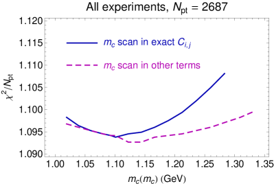
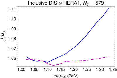
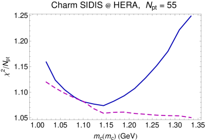
We have found that the global fit is sensitive to the exact charm mass, despite the introduced approximations. In one exercise, we have varied the input charm mass in the exact DIS coefficient functions for flavor-creation processes, while keeping it fixed in the above auxiliary mass scales. In a complementary exercise, we varied the input mass in all auxiliary scales, while keeping it fixed in the exact flavor-creation coefficient functions. In both cases, we examined the agreement with the data as a function of the varied mass parameter. We followed the fitting procedure outlined in the next section and assumed fixed PDF parametrizations for the best-fit $m_{c}(m_{c})$ found in the main analysis.

The dependence of the figure-of-merit function $\chi^{2}$ on the varied $m_{c}(m_{c})$ in these exercises is shown for all fitted experiments, the combined HERA inclusive DIS data Aaron et al. (2010a), and the combined HERA semi-inclusive charm production data Abramowicz et al. (2012) in the upper left, upper right, and lower panels of Fig. 1. To better visualize the comparison, $\chi^{2}$ is divided by the number $N_{pt}$ of data points for each data set. The solid blue line and dashed magenta line are for $\chi^{2}/N_{pt}$ for the varied mass parameter in the exact DIS coefficient functions and in the auxiliary mass scales, respectively.

With all PDF parameters fixed, variations in $\chi^{2}$ are more pronounced in the mass scan of the first type, when the charm mass is varied only in the exact DIS coefficient functions. In this case, $\chi^{2}$ in both inclusive and semiinclusive DIS shows a pronounced minimum as a function of $m_{c}(m_{c})$.

In the second case, when $m_{c}(m_{c})$ is varied only in the auxiliary scales, the $\chi^{2}$ dependence is flatter and has a shallow minimum at most. This exercise indicates that both inclusive and semiinclusive DIS cross sections are more sensitive to the exact $m_{c}$ mass in the flavor-creation coefficient functions than to the auxiliary scales. The detailed constraints on $m_{c}$ are determined by the interplay of these two trends as well as by variations in the PDFs and other inputs.

Figure 1: Dependence of $\chi^{2}/N_{pt}$ as a function of $m_{c}(m_{c})$ in the exact flavor-creation coefficient functions (solid blue lines) and auxiliary energy scales listed in the text (dashed magenta lines).

II.2 Details of implementation

II.2.1 Conversion to the pole mass

Our calculation proceeds by taking the $\overline{\rm MS}$ quark masses as the input for the whole calculation. The transition from the 3-flavor to 4-flavor evolution in $\alpha_{s}$ and PDFs is taken to occur at the scale equal to this input mass.

The massive 2-loop contributions to neutral-current DIS include matrix elements with explicit creation of $c\bar{c}$ pairs Riemersma et al. (1995) and operator matrix elements $A_{ab}^{(k)}$ Buza et al. (1998) for collinear production of massive quarks. Their available expressions take the pole mass as the input. For these parts, the $\overline{\rm MS}$ mass is converted to the pole mass according to the perturbative relation in Eq. (17) of Chetyrkin et al. (2000),

$$m^{pole}_{Q} = m_{Q}(m_{Q})\ \Biggl{\{}1+\frac{\alpha_{s}(m_{Q}(m_{Q}),N_{f})}{\pi}\frac{4}{3}$$ (1)

$$+ \frac{\alpha_{s}^{2}(m_{Q}(m_{Q}),N_{f})}{\pi^{2}}\Bigl{[}13.4434-1.04137N_{f}+\frac{4}{3}\sum_{i=1}^{N_{f}}\Delta(m_{i}(m_{i})/m_{Q}(m_{Q}))\Bigr{]}\Biggr{\}},$$

where $\Delta(x)=1.2337\ x-0.597\ x^{2}+0.23\ x^{3}$, and the coefficients are shown up to order $\alpha_{s}^{2}$.

For the charm quark, the $\alpha_{s}$ and $\alpha_{s}^{2}$ contributions in the conversion formula have comparable magnitudes, the procedure for $m_{c}^{pole}$ truncation is numerically important. We implement two conversion methods. In one method, the $\overline{\rm MS}$ mass is always converted to the pole mass via the full 2-loop relation. Alternatively, the 2-loop (1-loop) conversion is performed within the ${\cal O}(\alpha_{s})$ and ${\cal O}(\alpha_{s}^{2})$ terms of the Wilson coefficient functions and OME’s, respectively. This is argued to be equivalent to calculating DIS structure functions directly in terms of the $\overline{{\rm MS}}$ mass and improve perturbative convergence of the $m_{c}(m_{c})$ fit Alekhin and Moch (2011). Numerically, it is not obvious yet that the second (truncated) method improves perturbative convergence at the implemented orders: the effect of including an approximate 3-loop correction in the second method Alekhin et al. (2012) (producing the change $\delta m_{c}(m_{c})\approx 0.09$ GeV compared to the 2-loop result) exceeds the difference between two conversion methods at two loops ($\delta m_{c}(m_{c})\approx 0.07$ GeV).

In charged-current DIS, for which only 1-loop expressions are included, we can use either the $\overline{\rm MS}$ mass or pole mass and find almost no sensitivity to the choice.

II.2.2 Rescaling variable

The general-mass schemes Buza et al. (1998); Chuvakin et al. (2000); Thorne and Roberts (1998a, b); Thorne (2006); Forte et al. (2010) differ primarily in the form of approximation for flavor-excitation coefficient functions (with incoming heavy quarks) at $Q$ comparable to $m_{c}$. When $m_{c}$ is negligible, the coefficient functions in all GM-VFN schemes reduce to unique zero-mass expressions, but, near the threshold, they may differ by powerlike contributions $(m_{c}^{2}/Q^{2})^{p}$ with $p>0$ in the approximate flavor-excitation terms. The powerlike corrections are suppressed in the full result by an additional power of $\alpha_{s}$, i.e., they are of order $\alpha_{s}^{3}$ in an NNLO ($\alpha_{s}^{2}$) calculation.

In the S-ACOT-$\chi$ scheme, the form of the powerlike contributions is selected based on the general consideration of energy-momentum conservation Tung et al. (2002, 2007); Nadolsky and Tung (2009). As a result, the flavor-excitation contributions are suppressed at energies close to the massive quark production threshold, producing better description of the DIS data. The flavor-excitation coefficient functions are constructed from the respective zero-mass coefficient functions $c_{ZM}(\chi/\xi,Q/\mu)$, where the parton’s momentum fraction $\chi$ is rescaled with respect to Bjorken $x$ by a factor dependent on the total mass $M_{f}$ of heavy quarks in the final state. The general behavior of $\chi$ is determined from the condition of the threshold suppression, while its detailed form can be varied to estimate the associated higher-order uncertainty in the extracted $m_{c}$. This approach is readily demonstrated Guzzi et al. (2012) to be compliant with the QCD factorization theorem for DIS cross sections to all orders Collins (1998), which is one of the advantages of using the S-ACOT-$\chi$ scheme.

In the default implementation, the momentum fraction in NC DIS charm production is given by $\chi=x(1+4m_{c}^{2}/Q^{2})$, corresponding to $M_{f}=2m_{c}$ for the lightest final state ($c\bar{c}$). In charged-current DIS, we set $\chi=x\left(1+m_{c}^{2}/Q^{2}\right)$. The rescaling ratio $\chi/x$ is thus independent of $x$. On general grounds, it may be expected that the threshold suppression is less pronounced at $W^{2}=Q^{2}(1/x-1)\rightarrow\infty$ for fixed $Q$, corresponding to $x\rightarrow 0$. In this limit, it may be desirable to reduce or even eliminate the rescaling altogether, as quasi-collinear production of heavy quarks becomes more feasible.

To allow for this possibility, a generalized rescaling variable $\zeta$ can be implicitly defined by Nadolsky and Tung (2009)

$$x=\zeta\,\left(1+\zeta^{\lambda}M_{f}^{2}/Q^{2}\right)^{-1},$$

where $\lambda$ is a positive parameter, typically $0\leq\lambda\lesssim 1$. The S-ACOT-$\chi$ scheme is reproduced with $\lambda=0$, and the rescaling is fully turned off for $\lambda\gg 1$. For $\lambda\neq 0$, the mass-threshold constraints are enforced at small $W$ (large $x$), but the standard $x$ variable is recovered at large $W$ (small $x$) in a controllable way.

The sensitivity of the CTEQ global fit to $\lambda$ is of the same order as the sensitivity to the $m_{c}^{pole}$ truncation method. The changes in the preferred value of $m_{c}$ that we observe provide an estimate of the uncertainty due to the powerlike corrections.

III Charm mass scans

III.1 Setup

Using the theoretical setup reviewed in the previous section and the general procedure of the CT10 NNLO PDF analysis Gao et al. (2013), a scan of the log-likelihood function $\chi^{2}$ over the input $\overline{\rm MS}$ charm mass was carried out in the range $1\leq m_{c}(m_{c})\leq 1.4$ GeV. Besides the combined HERA data on inclusive DIS and semiinclusive charm production, we include experimental data from DIS measurements by BCDMS Benvenuti et al. (1989, 1990), NMC Arneodo et al. (1997), CDHSW Berge et al. (1991), and CCFR Yang et al. (2001); Seligman et al. (1997); NuTeV and CCFR dimuon production Goncharov et al. (2001); Mason (2006); $F_{2c}$ measurements at HERA Adloff et al. (2002) that are not included in the combined set; fixed-target Drell-Yan  process Moreno et al. (1991); Towell et al. (2001); Webb et al. (2003); vector boson and inclusive jet production at the Tevatron Abe et al. (1996); Acosta et al. (2005); Abazov et al. (2008a, b, c); Aaltonen et al. (2010, 2008); Abazov et al. (2008d). We also include inclusive jet production at the LHC Aad et al. (2012a, b), which slightly reduces the uncertainty in the gluon PDF.

Depending on the candidate fit, the QCD coupling strength was taken to be either the world average, $\alpha_{s}(M_{Z})=0.118$ Beringer et al. (2012), or a lower $\alpha_{s}(M_{Z})=0.115$, which is preferred by the CT10 NNLO analysis when $\alpha_{s}(M_{Z})$ is allowed to vary. The factorization/renormalization scale $\mu$ in DIS was set equal to the momentum transfer $Q$. To test the sensitivity to the PDF parametrization form, the initial scale $Q_{0}$ at which the input PDFs are provided was either set to be $Q_{0}=1$ GeV independently of $m_{c}$ or varied in the scan together with $m_{c}$ as $Q_{0}=m_{c}-0.005$ GeV. Several forms of the gluon PDF parametrization were considered, since DIS charm production is sensitive to the gluon PDF $g(x,Q)$. At the initial scale $Q_{0}$, we either constrained $g(x,Q_{0})$ to be positive at all $x$ or allowed it to be negative at small $x$, provided the negative gluon did not lead to unphysical predictions. In the latter case of the negative gluon, the fit included the H1 data on the longitudinal structure function $F_{L}(x,Q)$ Aaron et al. (2011a) and an additional theoretical constraint to ensure positivity of $F_{L}(x,Q)$ at $x>10^{-5}$.

III.2 Sensitivity of individual experiments

Figure 2: Individual $\chi^{2}$ contributions of the combined HERA-1 inclusive DIS data, NMC $F_{2}^{p}$ data, and combined HERA charm quark production data as a function of $m_{c}(m_{c})$.

Among all experiments included in the mass scan, the tightest constraints on $m_{c}$ are imposed by the inclusive DIS HERA data Aaron et al. (2010a) and HERA charm production Abramowicz et al. (2012). Weaker constraints also arise from the other DIS experiments, notably the NMC measurement of $F_{2}^{p}(x,Q)$.

Fig. 2 shows a sample of behavior of $\chi^{2}$ in each of three experiments as a function of $m_{c}$. The inclusive DIS data from HERA (upper left inset) and NMC (upper right inset) broadly prefer an $m_{c}$ in the range 1.1-1.3 GeV, while the charm HERA data (upper right inset) prefers lower $m_{c}$ values of order 1 GeV. The NMC shown in the lower inset prefers a higher $m_{c}$ of order 1.2 GeV in accord with the inclusive HERA data, but with flatter $\chi^{2}$ dependence. While in the shown mass scan the inclusive DIS data prefer a higher $m_{c}$ value than in DIS charm production, the $\chi^{2}$ minimum in inclusive DIS may shift to lower values of about 1.05-1.1 GeV depending on the parametrization forms of the PDFs and other fit assumptions.

We note that the semiinclusive reduced cross sections on HERA charm production were derived from charm differential distributions by applying a significant acceptance correction computed with the program HVQDIS Harris and Smith (1998) in the FFN scheme. Due to the mismatch in the schemes, the $m_{c}(m_{c})$ preferred by the HERA charm data may be biased when determined in the S-ACOT-$\chi$ general-mass scheme. Nevertheless, we see from Fig. 2 that the $m_{c}(m_{c})$ values that are separately preferred by the inclusive DIS and charm DIS data sets are about the same. In another cross check, we used separate, rather than combined, data sets for HERA charm production Chekanov et al. (2009, 2010); Aaron et al. (2010b, c); Aktas et al. (2007); Breitweg et al. (2000); Chekanov et al. (2004); Aaron et al. (2011b). Such fit did not differ much from the fit based on the combined HERA charm data set.

III.3 The global $\chi^{2}$ and PDF uncertainty

Figure 3: Global $\chi^{2}$ of the S-ACOT-$\chi$ NNLO fit as a function of the $\overline{{\rm MS}}$ charm mass. Lines with left/right arrows indicate 90% C.L. intervals obtained with different tolerance criteria.

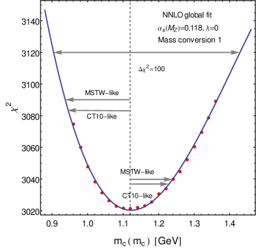
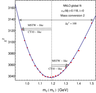
The constraints from various experiments are generally compatible and produce a well-defined minimum in the global $\chi^{2}$. The plots of $\chi^{2}$ for all experiments in the above $m_{c}(m_{c})$ scans is shown in Fig. 3 for the full $\overline{\rm MS}\rightarrow\mbox{pole}$ mass conversion (left inset) and truncated conversion (right inset). The PDF parameters were refitted for every $m_{c}(m_{c})$. The functional form for $\chi^{2}$ can be found in Ref. Gao et al. (2013). The default rescaling parameter $\lambda=0$ was used. The scattered points are for individual fits at discrete $m_{c}(m_{c})$ values, while the continuous line indicates smooth interpolation across the individual fits.

In the figure, the preferred value of the $\overline{{\rm MS}}$ charm mass, corresponding to the minimum of $\chi^{2}$, is $m_{c}(m_{c})=1.12$ GeV for the full conversion and 1.18 GeV for the truncated conversion. The optimal charm mass is below the world-average $m_{c}(m_{c})=1.275\pm 0.025$ GeV, and this general trend is observed in all fits.

From the mass dependence of $\chi^{2}$ in the figure, we can compute the uncertainty on $m_{c}(m_{c})$ due to the PDF parameters. Since the CT analysis traditionally operates with the 90% confidence level (90% C.L.) uncertainty, we compared 3 different criteria for defining it for $m_{c}(m_{c})$: 1) the uniform $\chi^{2}$ tolerance, in which one assigns a 90% C.L. to a $\Delta\chi^{2}\leq 100$ variation as in CTEQ6 Pumplin et al. (2002); 2) the CT10-like criterion, which supplements the uniform $\chi^{2}$ tolerance condition by additional $\chi^{2}$ penalties to prevent strong disagreements with individual experiments on average Lai et al. (2010a); 3) and the MSTW-like criterion, which does not introduce the uniform tolerance, but requires the $\chi^{2}$ value for every individual experiment to lie within the specified confidence interval. In the latter two methods, deviations of the PDF parameters are additionally constrained so as not to trigger a strong disagreement with one of the fitted experiments. This condition effectively reduces the PDF uncertainty in methods 2 and 3 compared to the uniform tolerance criterion (method 1), see further details in Lai et al. (2010a).

The PDF uncertainties on $m_{c}(m_{c})$ obtained with the three definitions are reported in Table 1. The uncertainty according to the uniform tolerance definition is larger than with the other two definitions, as anticipated.

PDF uncertainty $\delta m_{c}$ [GeV] (90% C.L.)
$\Delta\chi^{2}\leq 100$	$\delta m_{c}=_{-0.22}^{+0.30}$
CT10-like	$\delta m_{c}=_{-0.17}^{+0.11}$
MSTW-like	$\delta m_{c}=_{-0.18}^{+0.12}$

Table 1: The PDF uncertainty on the optimal value of $m_{c}$ extracted from the fit at the 90% C.L. by using three different criteria.

Figure 4: Total $\chi^{2}$ and its parabolic fit as functions the charm mass $m_{c}(m_{c})$.

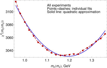
The rest of the paper interchangeably operates with the 68% and 90% C.L. intervals, with the former taken to be 1.65 times smaller than the latter. It is insightful to compare the above tolerance criteria to the procedure in the FFN analyses, Alekhin et al. (2012); Abramowicz et al. (2012) that assigns the 68% C.L. PDF uncertainty to the increase in the global $\chi^{2}$ by one unit. This definition of the PDF error Collins and Pumplin (2001); Bevington and Robinson (2002) is applicable under ideal conditions and leads to a smaller PDF error compared to the CT10 criterion. We have examined the $\Delta\chi^{2}=1$ criterion as an alternative to the CT10 criterion and found that it does not realistically describe the observed probability distribution. The reason is that the $\Delta\chi^{2}=1$ criterion is strictly valid when the experimental errors are Gaussian, which implies quadratic dependence of $\chi^{2}$ on $m_{c}(m_{c})$. The actual $\chi^{2}$ distribution is not perfectly Gaussian and exhibits asymmetry as well as some random fluctuations.

In Fig. 4 we compare the observed distribution of $\chi^{2}(m_{c,i})$ (scattered circles) with a fit by a second-degree polynomial $\chi^{2}_{parabola}(m_{c})=Am_{c}^{2}+Bm_{c}+C$ shown by the solid line. Deviations from the perfect quadratic behavior can be characterized by

$$X^{2}\equiv\sum_{i=1}^{N_{m_{c}}}(\chi^{2}_{parabola}(m_{c,i})-\chi^{2}(m_{c,i}))^{2},$$ (2)

where $N_{m_{c}}$ is the number of discrete $m_{c}(m_{c})$ values in the scan. In the ideal Gaussian case, when the individual $\chi^{2}(m_{c,i})$ follow neatly the parabola in the scanned $m_{c}(m_{c})$ region, $X^{2}$ is much less than $N_{m_{c}}-1$, and $\delta m_{c}=\sqrt{1/A}$ (about 0.025 GeV in our fits) provides a fair estimate of the $1\sigma$ error. But in the actual fits of the kind indicated by the circles in Fig. 4, $X^{2}/(N_{m_{c}}-1)$ is of order 2.5, hence $\sqrt{1/A}$ underestimates the $m_{c}$ error by a factor of about 2.5. This reflects the probability distribution that is broader than the ideal parabola and hence contains less than 68% of the net probability in the $m_{c}$ region where the parabolic growth results in $\Delta\chi^{2}=1$.

A partial remedy is procured by symmetric rescaling, if one defines $\widetilde{X}^{2}\equiv X^{2}/C$ with a constant $C\approx 2.5$ so that $\widetilde{X}^{2}\approx 1$ for the observed distribution of $\chi^{2}(m_{c,i})$. When the PDF uncertainty is derived from the rescaled $\widetilde{X}^{2}$ statistic, it is larger by a factor $C$ compared to the idealized assumption. Symmetric rescaling increases the 68% C.L. error but does not fix the shape of $\chi^{2}(m_{c})$. After the rescaling, the PDF error of 0.06 GeV gets closer to the one obtained by the CT10-like criterion, which is of order 0.09 GeV at 68% C.L. if the asymmetric errors are averaged over.

Our main conclusion is that, in the contest of our NNLO extraction of $m_{c}(m_{c})$, the quadratic assumption fails to describe the actual $\chi^{2}(m_{c}(m_{c})$ distribution to the extent needed to justify the $\Delta\chi^{2}=1$ prescription. The actual distribution is flatter near the minimum, asymmetric, and has occasional fluctuations. A number of reasons can explain this behavior. It has been observed in the earlier work Lai et al. (2010a); Pumplin (2009, 2010) that moderate disagreements between the fitted experiments broaden the probability distribution around the global minimum of $\chi^{2}$ compared to the ideal Gaussian case. The net effect of these disagreements may be approximated, to the first order, by increasing the $\Delta\chi^{2}=1$ PDF error by a factor of two or three, i.e., about the same factor as in the $m_{c}(m_{c})$ fit.

III.4 Systematic uncertainties

Theoretical systematic uncertainty	$m_{c}^{pole}$ conversion	DIS scale	$\alpha_{s}(M_{Z})$	$\lambda$	$\chi^{2}$ definition
Parameter range	–	$[Q/2,\ 2Q]$	[0.116,  0.120]	[0, 0.2]	–
$\delta m_{c}(m_{c})$ (GeV)	0.07	${}^{+0.02}_{-0.02}$	${}^{+0.01}_{-0.01}$	${}^{+0.14}_{-0}$	0.06

Table 2: Shifts of the optimal value of the charm mass $m_{c}(m_{c})$ obtained by varying theoretical inputs.

In addition to the PDF uncertainty associated with experimental errors, Table 2 summarizes systematic uncertainties on $m_{c}(m_{c})$ associated with theoretical inputs, including the $\overline{\rm MS}\rightarrow\mbox{pole}$ conversion procedure, the factorization/renormalization scale, $\alpha_{s}(M_{Z})$, the $\lambda$ parameter in the rescaling variable, and implementation of experimental correlated systematic errors. The last source of uncertainty arises from the existence of several prescriptions for including correlated systematic errors from the fitted experiments into the figure-of-merit function $\chi^{2}$ Ball et al. (2012b); Gao et al. (2013). Depending on the prescription, the relative correlated errors published by the experiments can be interpreted as fractions of either central data values or theoretical values. These methods are designated as “extended T” and “D” methods in Ref. Gao et al. (2013). This leads to numerical differences in absolute correlated errors, which may affect the outcomes of the fit, as discussed in the above references. We estimate the associated uncertainty by alternating between the two normalization methods for the correlation matrices of the DIS processes.

Figure 5: Comparison of the $\overline{\textrm{MS}}$ charm mass and its uncertainty extracted with various methods. Illustrated are also $m_{c}(m_{c})$ values obtained in an FFN analysis by Alekhin et al. Alekhin and Moch (2011).

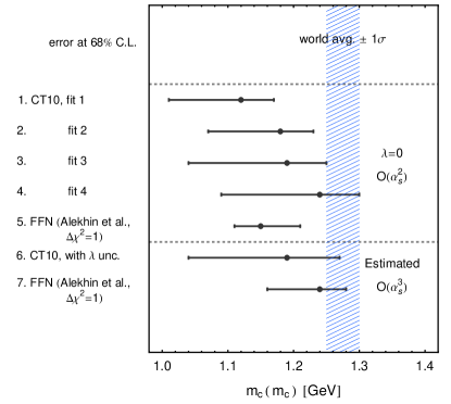
The values of $m_{c}(m_{c})$ obtained under various assumptions are illustrated by Fig. 5. At order $\alpha_{s}^{2}$, the highest fully implemented order in our calculation, we show $m_{c}(m_{c})$ found with four methods. Methods 1 and 2 correspond to the “extended $T$” and “experimental” $\chi^{2}$ definitions respectively Gao et al. (2013), both using the full $\overline{{\rm MS}}\rightarrow\mbox{pole}$ mass conversion formula, and $\lambda=0$. Methods 3 and 4 are the same as 1 and 2, but with truncated mass conversion equivalent to computing the coefficient functions in the $\overline{\rm MS}$ scheme. The resulting $m_{c}(m_{c})$ values in the four methods are $1.12^{+0.05}_{-0.11}$, $1.18^{+0.05}_{-0.11}$, $1.19^{+0.06}_{-0.15}$ and $1.24^{+0.06}_{-0.15}$ GeV, respectively. Here and in the figure we quote the 68% C.L. PDF uncertainties defined as in the CT10 analysis, cf. Sec. III.3.

The dependence on the $\lambda$ parameter is illustrated by Fig. 6, showing boundaries of the 68% and 90% C.L. regions when $\lambda$ takes values on the horizontal axis, for the “extended $T$” (solid lines) and “experimental” (dashed lines) definitions of $\chi^{2}$, and using the full $\overline{\rm MS}\rightarrow\mbox{ pole}$ conversion. The red empty triangle and black diamond symbols are the best-fit values of $m_{c}(m_{c})$ obtained with the two $\chi^{2}$ prescriptions, equal to 1.12 and 1.18 GeV, and reached when $\lambda\approx 0$ in both cases. Values of $\lambda$ above 0.14 and 0.20 are disfavored at 68% (90%) C.L. Finally, the horizontal blue band indicates the world-average interval $m_{c}(m_{c})=1.275\pm 0.025$ GeV.

Figure 6: Preferred regions for $m_{c}(m_{c})$ vs. the rescaling parameter $\lambda$. The best-fit values and confidence intervals are shown for two alternative methods for implementation of correlated systematic errors.

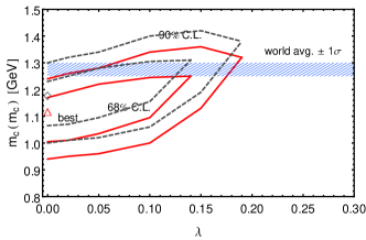
As we see, there is some spread in the $m_{c}$ values depending on the adopted $\overline{\rm MS}\rightarrow\mbox{pole}$ conversion and $\chi^{2}$ definition. In addition, moderate dependence exists on the rescaling parameter $\lambda$, associated with missing higher-order corrections. We can estimate the projected range for the ${\cal O}(\alpha_{s}^{3})$ value of $m_{c}(m_{c})$ in method 3 (or any other method) according to the CT10-like criterion from the $\chi^{2}$ dependence for a range of $\lambda$ values. This produces $1.19^{+0.08}_{-0.15}$ GeV for the estimated ${\cal O}(\alpha_{s}^{3})$ value in method 3, as shown in line 6 in Fig. 5. Here the errors are estimated from the 68% C.L. contour for $\chi^{2}$ vs. $\lambda$, and the scale and $\alpha_{s}$ errors are added in quadrature.

The central $m_{c}(m_{c})$ is consistent with the PDG value of $1.275\pm 0.025$ GeV Beringer et al. (2012) within the errors. A tendency of the fits to undershoot the PDG value may be attributable to the missing ${\cal O}(\alpha_{s}^{3})$ contribution Alekhin et al. (2012). The results of our fit are compatible with $m_{c}(m_{c})$ determined in the (FFN) scheme Alekhin et al. (2012) both at the exact ${\cal O}(\alpha_{s}^{2})$ and approximate ${\cal O}(\alpha_{s}^{3})$, cf. lines 5 and 7 in Fig. 5. However, our PDF error of about 0.08 GeV is 2.7 times larger than the one quoted in the FFN study. The main reason is that the 68% C.L. PDF uncertainty of the FFN analysis corresponds to $\Delta\chi^{2}=1$ and hence is smaller than the CT10-like uncertainty. As discussed above, our $\chi^{2}$ dependence on $m_{c}(m_{c})$ is not compatible with the ideal Gaussian behavior and could be accommodated by increasing the PDF error by a factor 2-3 compared to the $\Delta\chi^{2}=1$ definition. Besides this difference in the PDF uncertainty, the results for $m_{c}(m_{c})$ from the S-ACOT-$\chi$ and FFN fits are in general agreement.

Figure 7: Relative changes in select PDFs $f_{a/p}(x,Q)$ at $Q=2$ GeV obtained in a series of PDF fits with $m_{c}(m_{c})$ ranging from 1 to 1.36 GeV, plotted as ratios to the respective PDFs for $m_{c}(m_{c})=1$ GeV. Default rescaling ($\lambda=0$) in DIS coefficient functions is assumed. Darker colors correspond to larger $m_{c}(m_{c})$ values.

III.5 Implications for PDFs and collider observables

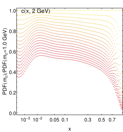
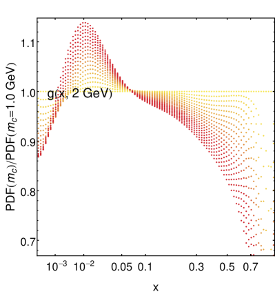
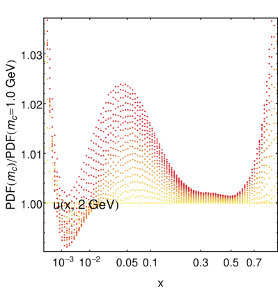
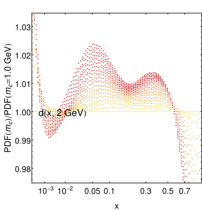
As $m_{c}(m_{c})$ changes in the mass scan, parametrizations of the PDFs are adjusted so as to maximize agreement with the data. Representative best-fit PDFs from a charm mass scan are plotted in Fig. 7 at $Q=2$ GeV. In this example, we vary the charm mass in the interval $1.0\leq m_{c}(m_{c})\leq 1.36$ GeV that is about the same as the 90% C.L. CT10-like PDF uncertainty determined in the previous section. For each $m_{c}(m_{c})$ from this range, we refit the PDFs, while keeping the other theoretical inputs at their default values, in particular assuming $\alpha_{s}(M_{Z})=0.118$ and $\lambda=0$ in the rescaling variable. Darker color points in Fig. 7 correspond to larger mass values.

In general, as the charm mass is increased, both the charm PDF (upper left subfigure) and charm contributions to DIS cross sections are suppressed. Consequently, the gluon PDF (upper right subfigure) is enhanced in the intermediate $x$ region, $10^{-3}\sim 10^{-2}$ so as to partly compensate for this reduction. This is accompanied by moderate enhancements in the up and down quark PDFs (lower subfigures) at $x\approx 10^{-2}-0.5$ and slight suppression of the same PDFs at $x\approx 10^{-3}$.

Figure 8: Plot of NNLO cross sections for $W^{\pm}$, $Z^{0}$, Higgs boson production through gluon fusion, and top quark pair production at the LHC (8 TeV) for charm quark mass $m_{c}(m_{c})$ ranging from 1 to 1.36 GeV and $\lambda=\{0,\ 0.02,\ 0.05,\ 0.1,\ 0.15,\ 0.2\}$. Darker color corresponds to larger mass values. The black boxes represent the cross sections evaluated by using $m_{c}(m_{c})=1.28$ (close to world average) GeV and the explored $\lambda$ values. The empty triangle and ellipse indicate the central predictions and its 90% C.L. interval based on the CT10NNLO fit.

Figure 9: Same as in Fig. 8, but with $\sqrt{S}=14$ TeV.

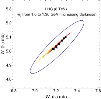
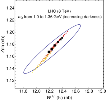
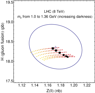
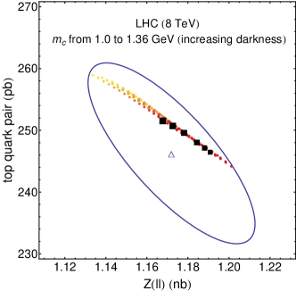
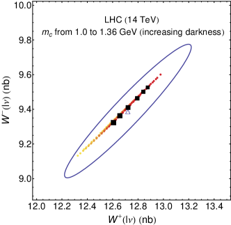
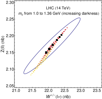
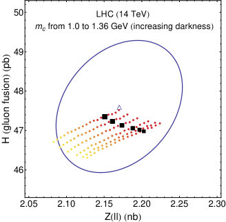
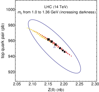
PDF variations of such magnitude may have impact on collider observables Nadolsky et al. (2008). For example, in Fig. 8 and 9 we show the dependence of NNLO total cross sections for $W,$ $Z,$ Higgs boson production through gluon fusion, and top quark pair production at the LHC at $\sqrt{S}=8$ and $14$ TeV. The NNLO cross sections for $W$ and $Z$ production are computed using FEWZ2.1 Gavin et al. (2011, 2012). The NNLO cross sections for Higgs and top quark pair production are obtained from iHixs1.3 Anastasiou et al. (2011) and Top++2.0 Baernreuther et al. (2012); Czakon et al. (2013) with $m_{h}=125\ {\rm GeV}$, $m_{t}=173.3\ {\rm GeV}$, and the QCD scales set to the corresponding mass values. For each pair of total cross sections, we show the central CT10NNLO prediction and an ellipse corresponding to the 90% C.L. PDF uncertainty interval of the CT10NNLO set Gao et al. (2013). In the same figure, scattered points indicate the cross sections obtained with various combinations of $m_{c}(m_{c})$ and $\lambda$ in the intervals $1\leq m_{c}(m_{c})\leq 1.36$ GeV and $0\leq\lambda\leq 0.2$. Here the darker colors represent larger values of $m_{c}$, as in Fig. 7. The $W$, $Z$, and Higgs production cross sections increase with the charm mass by a few percent in the mass range considered. The trend is opposite for $t\bar{t}$ production. The changes are contained within the CT10NNLO PDF uncertainty ellipse, however, and do not modify the PDF-induced (anti-)correlations observed between the shown total cross sections.

The shown uncertainty in the LHC cross sections due to $m_{c}$ is comparable to the experimental PDF uncertainty and in principle should be included independently from the latter. Let us outline one possibility for reducing the $m_{c}$ uncertainty. Instead of allowing $m_{c}(m_{c})$ to vary in the whole interval $1-1.36$ GeV of its PDF uncertainty, we could set it to be at the world-average $m_{c}(m_{c})$ value of 1.275 GeV or in the $1\sigma$ interval $\pm 0.025$ GeV around it. This would reduce the associated uncertainty in the PDFs and QCD observables. The corresponding predictions for the LHC $W,$ $Z,$ Higgs, and top quark pair production cross sections, obtained for $m_{c}(m_{c})=1.28$ GeV and five explored $\lambda$ values, are shown in Figs. 8 and 9 by black boxes, with the size of the boxes increasing with the value of $\lambda$. The spread in these predictions constitutes only a part of the full span covered by the scattered points for the interval $1\leq m_{c}\leq 1.36$ GeV. It reflects only the uncertainty due to the form of the rescaling variable, controlled by the $\lambda$ parameter. Theoretical predictions are better clustered in this case.

IV Conclusions

We explored the charm quark mass dependence in the CTEQ NNLO global PDF analysis that includes the recently published combined data on charm quark production at the $ep$ collider HERA. This analysis, carried out in the S-ACOT-$\chi$ heavy-quark scheme at order $\alpha_{s}^{2}$, renders an optimal $\overline{\rm MS}$ charm mass that is compatible with the world-average value $m_{c}(m_{c})=1.275\pm 0.025$ GeV. For example, with the $\overline{\rm MS}$ Wilson coefficient functions for NC DIS, we obtain $m_{c}(m_{c})=1.19^{+0.08}_{-0.15}\mbox{ GeV}$, where the errors indicate the 68% C.L. uncertainty due to the PDFs and variation of the rescaling variable, as well as the scale and $\alpha_{s}$ uncertainties added in quadrature.

In QCD predictions for massive-quark DIS, one draws a distinction between the $\overline{\rm MS}$ charm mass, the fundamental parameter of the QCD Lagrangian, and auxiliary energy scales of order of the physical charm mass. The auxiliary scales that can contribute are specified by the factorization scheme. They can be associated with the evolution of the QCD coupling strength, evolution of PDFs, heavy-quark fragmentation, and powerlike contributions $(m_{c}/Q)^{p}$ in DIS coefficient functions with initial-state charm quarks.

We argue that the sensitivity to the auxiliary scales is reduced as the order of the PQCD calculation increases. In support of this argument, Fig. 1 demonstrates that the DIS data are sensitive mostly to the physical mass parameter in the exact DIS coefficient functions and less to the auxiliary mass scales in the other parts of the calculation. Thus, the hadronic cross sections in DIS and other processes at NNLO and beyond become increasingly suitable for the determination of the fundamental charm mass.

The main findings of our fit are summarized in Fig. 5 showing the 68% C.L. intervals for the $\overline{\rm MS}$ charm mass obtained under various assumptions explained in the text. The central value of $m_{c}(m_{c})$ in the S-ACOT-$\chi$ scheme at two loops tends to undershoot the world-average value according to the figure, but is compatible with the latter within the uncertainty.

The uncertainties in the $m_{c}(m_{c})$ determination of both experimental and theoretical origin were explored in Sec. III. If $m_{c}(m_{c})$ is varied as an independent parameter in the full range of order 1-1.4 GeV allowed by the NNLO PDF fit, it increases the uncertainty on the resulting PDFs, compared to a fixed $m_{c}$.

For comparison, the accuracy of the world-average $m_{c}(m_{c})$, at about $0.025$ GeV, is smaller than the NNLO fit uncertainty. By using a constant value of the $m_{c}(m_{c})$ parameter, for example by setting it equal to its world-average value, one can suppress the corresponding uncertainty in the PDFs. This strategy is similar to implementing the QCD coupling dependence in the global analysis Lai et al. (2010b), when using the world-average value of $\alpha_{s}(M_{Z})=0.118$ results in tighter constraints on the PDFs than in a fit with a free $\alpha_{s}(M_{Z})$. When the input $m_{c}(m_{c})$ value is held constant instead of being fitted, one suppresses the associated uncertainty in the PDFs and LHC cross sections, see sample calculations in Figs. 8 and 9. The residual theoretical uncertainty for a fixed $m_{c}(m_{c})$ then arises only from variations in the auxiliary scales and powerlike contributions and can be suppressed by including higher orders in $\alpha_{s}$.