Cross-Validation for Nonlinear Mixed Effects Models

Abstract

Cross-validation is frequently used for model selection in a variety of applications. However, it is difficult to apply cross-validation to mixed effects models (including nonlinear mixed effects models or NLME models) due to the fact that cross-validation requires “out-of-sample” predictions of the outcome variable, which cannot be easily calculated when random effects are present. We describe two novel variants of cross-validation that can be applied to nonlinear mixed effects models. One variant, where out-of-sample predictions are based on post hoc estimates of the random effects, can be used to select the overall structural model. Another variant, where cross-validation seeks to minimize the estimated random effects rather than the estimated residuals, can be used to select covariates to include in the model. We show that these methods produce accurate results in a variety of simulated data sets and apply them to two publicly available population pharmacokinetic data sets.

1 Introduction

1.1 Overview of Population Pharmacokinetic and Pharmacodynamic Modeling

Population pharmacokinetic and pharmacodynamic (PK/PD) modeling is the characterization of the distribution of probable PK/PD outcomes (parameters, concentrations, responses, etc) in a population of interest. These models consist of fixed and random effects. The fixed effects describe the relationship between explanatory variables (such as age, body weight, or gender) and pharmacokinetic outcomes (such as the concentration of a drug). The random effects quantify variation in PK/PD outcomes from individual to individual.

Population PK/PD models are hierarchical. There is a model for the individual, a model for the population, and a model for the residual error. The individual PK model typically consists of a compartmental model of the curve of drug concentrations over time. The pharmacokinetic compartmental model is similar to a black box engineering model. Each of the compartments is like a black box, where a system of differential equations is derived based on the law of conservation of mass (Sandler, 2006). The number of such compartments to include in the model must be determined based on the data.

The equations for the PK/PD parameters represent the model for the population in the hierarchy of models. The PK/PD parameters are modeled with regression equations containing fixed effects, covariates, and random effects (denoted by $\eta$’s). The random effects account for the variability across subjects in the parameters and for anything left out of the parameter equations (such as a covariate not included). The vector of random effects ($\eta$) is assumed to follow a multivariate normal distribution with mean 0 and variance-covariance matrix $\Omega$. The matrix $\Omega$ may be diagonal, full block, or block diagonal. The model for the residual error ($\epsilon$) accounts for any deviation from the model in the data not absorbed by the other random effects. The residual error model may be specified such that measurements with higher values are given less importance compared with measurements with smaller values, often referred to as “weighting”.

Hence, population PK/PD models are non-linear mixed effects (NLME) models. They are represented by differential equations that may or may not have closed-form solutions, and are solved either analytically or numerically. The parameters are estimated using one of the various algorithms available such as first order conditional estimation with interaction (FOCEI). See Wang (2007) for a mathematical description of these algorithms.

Once model parameters are estimated using an algorithm such as FOCEI, one may fix the values of the model estimates and perform a post hoc calculation to obtain random effect values ($\eta$’s) for each subject. Thus, one may fit a model to a subset of the data and obtain random effect values for the full data set. See Wang (2007) for a discussion of how these posterior Bayes (post hoc) estimates of the $\eta$’s are calculated.

1.2 Cross-Validation and Nonlinear Mixed Effects Modeling

In general, cross-validation is not frequently used for evaluating nonlinear mixed effects (NLME) models (Brendel et al, 2007). When cross-validation is applied to NLME models, it is generally used to evaluate the predictive performance of a model that was selected using other methods. For example, in Bailey et al (1996), data were pooled across subjects to fit a model as though the data were obtained from a single subject. Subjects were removed one at a time, and the accuracy of the predicted observations with subsets of the data was assessed. Another approach (Hooker et al, 2008) removed subjects one at a time to estimate model parameters and predicted PK parameters using the covariate values for the subject removed. The parameters were compared with the PK parameters obtained using the full data set in order to evaluate the final model and identify influential individuals. See Mulla et al (2003), Kerbusch et al (2001), and Rajagopalan and Gastonguay (2003) for additional examples where cross-validation was used to validate NLME models.

Less frequently cross-validation is used for model selection in NLME modeling. For example, one may wish to compare a model with a covariate to another model without the covariate. In Ralph et al (2006), the prediction error of the posterior PK parameter for each subject was calculated, and a paired t-test was performed to compare the prediction error between a base and full model to assess whether differences between the models were significant. The full model was only found to be correct when the effect of the covariate was large.

In several published studies, cross-validation failed to identify covariate effects that were identified using other methods. As noted earlier, Ralph et al (2006) found that cross-validation only identified covariate effects when the effect was large. Similarly, Zomorodi et al (1998) found that cross-validation tended to favor a base model (without a covariate) despite the fact that the covariate was found to be significant using alternative approaches. Fiset et al (1995) also found that models with and without covariates tended to produce comparable error rates despite the fact that likelihood-based approaches favored models that included covariates. Indeed, Wahlby et al (2001) used a special form of cross-validation where one concentration data point was chosen for each parameter, which was the point at which the parameter was most sensitive based on partial derivatives. Once again, little difference was observed between models that included covariates and corresponding models without covariates. Thus, cross-validation can fail to detect covariate effects even when attention is restricted to a subset of the data that should be most sensitive to model misspecification.

Despite the fact that cross-validation may fail to detect covariate effects, it has been successfully used to compare models with structural differences, such as a parallel Michaelis-Menten and first-order elimination (MM+FO) model and a Michaelis-Menten (MM) model (Valodia et al, 2000). This indicates that cross-validation can be used for model selection in NLME modeling under certain circumstances. Moreover, the fact that cross-validation often fails to detect covariate effects is not surprising. When covariate effects are present in an underlying NLME model, a misspecified model that fails to include a covariate may not significantly decrease the predictive accuracy of the model. This can occur when random effects in the pharmacokinetic parameters can compensate for the missing covariate. Thus, if cross-validation chooses the model with the lowest out-of-sample prediction error, it may not be able to determine whether a covariate should be included in the model.

Other methods have been proposed for using cross-validation for model selection in NLME modeling (Ribbing and Jonsson, 2001; Katsube et al, 2011). However, these methods rely on estimation of the likelihood function, which is unusual for cross-validation, and they have not been studied extensively.

Thus, we propose an alternative form of cross-validation for covariate model selection in NLME modeling. Rather than choosing a model which minimizes the out-of-sample prediction error, we choose a model which minimizes the post hoc estimates of the random effects ($\eta$’s). The motivation is that if the $\eta$’s are large, this suggests that there is a large amount of unexplained variation from individual to individual, which indicates that a covariate may be missing from the model. However, traditional cross-validation (which minimizes the out-of-sample prediction error) is still useful for comparing structural models, as we will discuss below.

2 Methods

2.1 Cross-Validation

Cross-validation is a method for evaluating the expected accuracy of a predictive model. Suppose we have a response variable $Y$ and a predictor variable $X$ and we seek to estimate $Y$ based on $X$. Using the observed $X$’s and $Y$’s we may estimate a function $\hat{f}$ such that our estimated value of $Y$ (which we call $\hat{Y}$) is equal to $\hat{f}(X)$. Cross-validation is an estimate of the expected loss function for estimating $Y$ based on $\hat{f}(X)$. If we use squared error loss (as is conventional in NLME modeling), then cross-validation is an estimate of $E\left[\left(Y-\hat{f}(X)\right)^{2}\right]$.

A brief explanation of cross-validation is as follows: First, the data is divided into $K$ partitions of roughly equal size. For the $k$th partition, a model is fit to predict $Y$ based on $X$ using the $K-1$ other partitions of the data. (Note that the $k$th partition is not used to fit the model.) Then the model is used to predict $Y$ based on $X$ for the data in the $k$th partition. This process is repeated for $k=1,2,\ldots,K$, and the $K$ estimates of prediction error are combined. Formally, let $\hat{f}^{-k}$ be the estimated value of $f$ when the $k$th partition is removed, and suppose the indices of the observations in the $k$th partition are contained in $K_{k}$. Then the cross-validation estimate of the expected prediction error is equal to

$$\frac{1}{n}\sum_{i=1}^{k}\sum_{j\in K_{i}}\left(y_{j}-\hat{f}^{-i}(x_{j})\right)^{2}$$

Here $n$ denotes the number of observations in the data set. For a more detailed discussion of cross-validation, see Hastie et al (2008).

The above procedure is known as $k$-fold cross-validation. Leave-one-out cross validation is a special case of $k$-fold cross-validation where $k$ is equal to the number of observations in the original data set.

2.2 Comparing covariate models

In some situations, a researcher may want to compare models with and without covariate effects, such as a model with an age effect on clearance versus a model without an age effect on clearance. This method is designed to detect differences in models that affect the equations for the parameters.

Consider a data set with subjects $i=1,2,\ldots,n$. Each subject has observations $y_{ij}$ for $j=1,2,\ldots,t_{i}$ (where $t_{i}$ is the number of time points or discrete values of the independent variable for which there are observations for subject $i$). The question of interest is whether or not a fixed effect $dPdX$ for a covariate $X$ should be included in an equation for a parameter $P$, having fixed effect $tvP$ and random effect $\eta_{P}$. The equation for $P$ could have any of the typical forms used in NLME modeling. For example, one could compare a model with a covariate $X$

$$P=tvP*(X/\operatorname{mean}(X))^{dPdX}*\exp(\eta_{P})$$ (1)

to a model having no covariate effect

$$P=tvP*\exp(\eta_{P})$$ (2)

If a covariate $X$ has an effect on a parameter $P$, the unexplained error in $P$ (modeled by $\eta_{P}$) when $X$ is left out of the model tends to have higher variance. By including covariate $X$ in the model, we wish to reduce the unexplained error in $P$, which is represented by $\eta_{P}$. Therefore, metrics involving $\eta_{P}$ are useful for determining whether a covariate $X$ is needed. Specifically, one can perform cross-validation to compare the predicted $\eta_{P}$’s when $X$ is included or not included in the model. We propose a statistic for determining whether a covariate, $X$, is needed for explaining variability in a parameter, $P$, when $P$ is modeled with a random effect $\eta_{P}$. The statistic can be calculated as follows:

For $i$ = 1 to $n$:

1. Remove subject $i$ from the data set.

2. Fit a mixed effects model to the subset of the data with subject $i$ removed.

3. Accept all parameter estimates from this model, and freeze the parameters to those values.

4. Fit the same model to the whole data set, without any major iterations, estimating only the post hoc values of the random effects. (In NONMEM, use the commands MAXITER=0, POSTHOC=Y. In NLME, set NITER to 0.)

5. Square the post hoc eta estimate for the subject that was left out for the parameter of interest

Take the average of the quantity in step 5 over all subjects.

This sequence of steps can also be represented by the equation

$$\text{CrV}_{\eta}=\frac{1}{n}\sum\limits_{i=1}^{n}(\hat{\eta}_{P_{i,-i}})^{2}$$ (3)

where $\hat{\eta}_{P_{i,-i}}$ is the post hoc estimate of the random effect for the $i$th subject for parameter $P$ in a model where the $i$th subject was removed, and $n$ is the number of subjects. Note that our method leaves out one subject at a time, rather than one observation at a time.

In general, one will favor the model with the minimum value of $\text{CrV}_{\eta}$. However, to avoid over-fitting, it is common when applying cross-validation to choose the most parsimonious model (i.e. the model with the fewest covariates) that is within one standard error (SE) of the model with minimum $\text{CrV}_{\eta}$ (Hastie et al, 2008). We will follow this convention in all of our subsequent examples. We define $\text{SE}(\text{CrV}_{\eta})$ as the sample standard deviation of the squared post hoc etas for the subjects left out divided by the square root of the number of subjects. The formula for $\text{SE}(\text{CrV}_{\eta})$ is given by

$$\text{SE}(\text{CrV}_{\eta})=\sqrt{\frac{1}{n(n-1)}\sum\limits_{i=1}^{n}(x_{i}-\bar{x_{i}})^{2}}$$ (4)

where

$$x_{i}=\hat{\eta}_{P_{i,-i}}^{2}$$ (5)

Alternatively, one may follow the same procedure while removing more than one subject at a time. For example, one may divide the data into $k$ roughly equally-sized partitions, fit a model using the data in $k-1$ of the partitions, and calculate the post hoc $\eta$ values for the subjects left out of the model. For data sets with large numbers of subjects, this approach is obviously faster than the “leave-one-out” approach, and it may also reduce the amount of variance in the cross-validation estimates (Hastie et al, 2008). However, this approach may not be practical if the number of subjects is small. We will only consider the leave-one-out method in our subsequent analysis.

2.3 Comparing models with major structural differences

In other situations, a researcher may want to compare models with major structural differences, such as a one compartment model and a two compartment model. This method is designed to detect differences in models that affect the overall shape of the response.

As discussed previously, consider a data set with subjects $i=1,2,\ldots,n$, where each subject has observations $y_{ij}$ for $j=1,2,\ldots,t_{i}$. The statistic can be calculated as follows:

For $i$ = 1 to $n$:

1. Remove subject $i$ from the data set.

2. Fit a mixed effects model to the subset of the data with subject $i$ removed.

3. Accept all parameter estimates from this model, and freeze the parameters to those values.

4. Fit the same model to the whole data set, without any major iterations, estimating only the post hoc values of the random effects. (In NONMEM, use the commands MAXITER=0, POSTHOC=Y. In NLME, set NITER to 0.)

5. Calculate predicted values for subject $i$ (the subject that was left out). Note that this estimate uses the post hoc estimate of the random effects for subject $i$.

6. Take the average of the squared individual residuals for the subject that was left out (over all time points or over all values of the independent variable $t_{i}$)

Take the average of the quantity in step 6 over all subjects.

This sequence of steps can also be represented by the equation

$$\text{CrV}_{y}=\frac{1}{n}\sum\limits_{i=1}^{n}\frac{\sum\limits_{j=1}^{t_{i}}(y_{ij}-\hat{y}_{ij,-i})^{2}}{t_{i}}$$ (6)

where $y_{ij}$ is the observed value for the $i$th subject at the $j$th time point or independent variable value and $\hat{y}_{ij,-i}$ is the predicted value for the $i$th subject at the $j$th time point or independent variable value in a model where subject $i$ is left out and post hocs are obtained. Once again, note that our method leaves out one subject at a time, rather than one observation at a time.

For purposes of exploration, another statistic that takes into account the weighting of the response can also be calculated:

$$\text{wtCrV}_{y}=\frac{1}{n}\sum\limits_{i=1}^{n}\frac{\sum\limits_{j=1}^{t_{i}}\text{WTIRES}_{ij,-i}^{2}}{t_{i}}$$ (7)

Here $\text{WTIRES}_{ij,-i}$ is the individual weighted residual for subject $i$ at time or independent variable value $j$ in a model where subject $i$ is left out and post hocs are obtained, which is defined to be:

$$\text{WTIRES}_{ij,-i}=\frac{\sqrt{wt_{ij,-i}}(y_{ij}-\hat{y}_{ij,-i})}{\hat{\sigma}_{-i}}$$ (8)

where $wt_{ij,-i}$ is the weight defined by the residual error model (equal to the squared reciprocal of $\hat{y}_{ij,-i}$ for constant CV error models or 1 for additive error models), and $\hat{\sigma}_{-i}^{2}$ is the estimated residual variance.

As discussed previously, we will follow the convention of choosing the most parsimonious model (defined to the model with the fewest number of compartments) within one standard error (SE) of the model with the minimum $\text{CrV}_{y}$. The formula for $\text{SE}(\text{CrV}_{y})$ is given by

$$\text{SE}(\text{CrV}_{y})=\sqrt{\frac{1}{n(n-1)}\sum\limits_{i=1}^{n}(x_{i}-\bar{x_{i}})^{2}}$$ (9)

where

$$x_{i}=\frac{\sum\limits_{j=1}^{t_{i}}(y_{ij}-\hat{y}_{ij,-i})^{2}}{t_{i}}$$ (10)

and the formula for $\text{SE}(\text{wtCrV}_{y})$ is calculated similarly, with

$$x_{i}=\frac{\sum\limits_{j=1}^{t_{i}}\text{WTIRES}_{ij,-i}^{2}}{t_{i}}$$ (11)

One may also consider $k$-fold cross-validation, although we will restrict our attention to leave-one-out for our subsequent analysis.

This method is similar to existing methods for cross-validation on NLME models. However, some applications of cross-validation do not use post hoc estimates of the outcome variable, which is an important difference from our proposed method. Also, we will show why this method should not be used for comparing covariate models.

2.4 Simulated Data Analysis

Five sets of simulated data were generated to evaluate the performance of our proposed cross-validation methods. In each simulation scenario, two models were compared: a sparser “base model” and a less parsimonious “full model.” The objective was to determine which of the two possible models was correct using cross-validation.

A brief description of the five simulation scenarios is given in Table 1. For a more detailed description of how the simulated data sets were calculated, see Section S1 in Online Resource 1. For simulation scenarios 1-4, 200 simulated data sets were generated using Pharsight’s Trial Simulator software version 2.2.1. (Only 100 simulated data sets were generated for scenario 5.) For each simulated data set, Pharsight’s Phoenix NLME (platform version 1.3) was used to fit the appropriate population PK models (both the base model and the full model) using the Lindstrom-Bates method (Lindstrom and Bates, 1990). The $\eta$ shrinkage of each model was calculated and diagnostics were performed to verify the convergence of each model. To calculate the cross-validation statistics for each simulated data set, subjects were removed from the data set one at a time and the models were recalculated with each subject removed. Post hoc estimates of the random effects (and corresponding predicted values of $y$) were then calculated for the subject that was excluded from the model. The values of $\text{CrV}_{\eta}$, $\text{CrV}_{y}$, and $\text{wtCrV}_{y}$ were obtained by averaging over each such model. The simulated data sets, batch files, Phoenix mdl files, and other files used to process the output are available from the authors by request.

Table 1: Description of the five simulation scenarios

Scen.	True Model	Base Model	Full Model
1	one compartment, no covariate effects	one compartment, no covariate effects	one compartment, age effect on clearance
2	one compartment, age effect on clearance	one compartment, no covariate effects	one compartment, age effect on clearance
3	two compartments, age effect on clearance	two compartments, no covariate effects	two compartments, age effect on clearance
4	one compartment, body weight effect on volume, body weight, age, gender, and hepatic impairment effects on clearance	one compartment, body weight effect on volume, body weight, age, and gender effects on clearance	one compartment, body weight effect on volume, body weight, age, gender, and hepatic impairment effects on clearance
5	two compartments, no covariate effects	one compartment, no covariate effects	two compartments, no covariate effects

For each simulated data set, the base model was selected if the value of $\text{CrV}_{\eta}$ for the base model was less than that of the full model. The full model was selected if the value of $\text{CrV}_{\eta}$ was less than that of the base model plus one standard error (using the convention that the more parsimonious model is preferable if its cross-validation error is within one standard error of the cross-validation error of a less parsimonious model). Similar decision rules were used for $\text{CrV}_{y}$ and $\text{wtCrV}_{y}$. The Akaike’s information criterion (AIC) (Akaike, 1974) and Bayesian information criterion (BIC) (Schwarz, 1978) were also calculated for the two models for each simulated data set. The model (base or full) with the smallest AIC/BIC was selected under the two criteria. For each scenario, the performance of cross-validation was compared to the performance of AIC/BIC using a two-sample proportion test.

Note: Consistent with the recommendations of Vonesh and Chinchilli (1997), the BIC was weighted by the number of observations. Although others have suggested that the BIC should be weighted by the number of subjects(Kass and Raftery, 1995), one recent simulation study found that neither choice of weight consistently outperforms the other when applied to mixed models (Gurka, 2006).

2.5 Indomethacin Data Analysis

Pharsight’s Phoenix NLME (version 1.3) was used to fit models to a previously published indomethacin data set (Kwan et al, 1976). The data consists of six subjects with 11 observations per subject. Each subject was administered a 25 mg dose of indomethacin intravenously at the beginning of the study, and the concentration of indomethacin was measured at 11 time points over an eight-hour period.

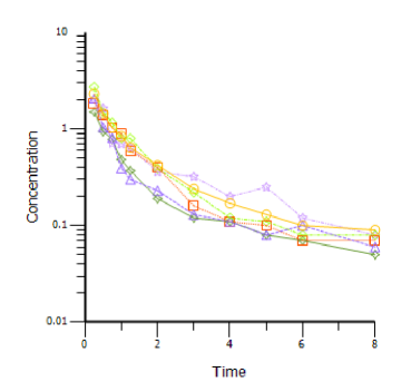
The concentrations were plotted versus time for each subject (see Figure 1). Based on the plot, a two compartment IV bolus model with clearance parametrization and a proportional residual error model was fit to this data set. See Section S3.1 in Online Resource 1 for a more detailed description of the model. Individual initial estimates were obtained using the curve stripping method (Gibaldi and Perrier, 1982) with a WinNonlin Classic model. The averages of the individual PK parameters were used as initial estimates for the pop PK model. Random effects were added to the PK parameters for systemic volume and clearance in the form $\theta P*\exp(\eta P)$, where $P$ is the parameter of interest. The Phoenix project file used to fit this model is available from the authors by request.

Figure 1: Concentration versus time profiles from the indomethacin data set

After fitting the model, a series of diagnostic plots were generated to assess the validity of the model. (See Section S3.2 in Online Resource 1 for details.) The model was then compared to a one compartment model based on both $\text{CrV}_{y}$ and a likelihood ratio test (LRT). First, the model was refit without including any random effects on the PK parameters. (The LRT cannot be used when the random effects are included in this case since the one compartment model forces the removal of some random effects, which implies that these random effects have variances of 0. Thus, comparing the two models would require testing the null hypothesis that a variance is equal to 0, which is on the boundary of the parameter space, rendering the LRT invalid. See Fitzmaurice et al (2011) for details.). The LRT was used to test the null hypothesis of no difference in the predictive accuracy of the two compartment model versus the one compartment model. The value of $\text{CrV}_{y}$ was also calculated for both models. Finally, the value of $\text{CrV}_{y}$ was calculated for a one compartment and two compartment version of the original model (with random effects included). See Section S3.1 in Online Resource 1 for a detailed description of the models that were considered.

2.6 Theophylline Data Analysis

Pharsight’s Phoenix NLME (version 1.3) was used to fit models to a published theophylline data set (Boeckmann et al, 1992). This theophylline data set consists of twelve subjects with eleven observations per subject. Each subject was administered a dose of theophylline at the beginning of the study ranging between 3.1 mg/kg and 5.86 mg/kg. The concentration of theophylline was measured at 11 time points per subject over a 24 hour period. Each subject’s weight was also recorded.

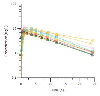
The concentration were plotted versus time for each subject (see Figure 2). Based on the plot, a one compartment extravascular model with clearance parametrization and an additive residual error model was fit to this data set. Random effects were added to the PK parameters for absorption rate, and systemic volume and clearance in the form $\theta P*\exp(\eta P)$, where $P$ is the parameter of interest. See Section S3.1 in Online Resource 1 for a more detailed description of the model. The Phoenix project file used to fit this model is available from the authors by request.

Figure 2: Concentration versus time profiles from the theophylline data set

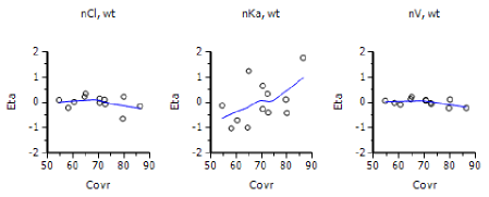
The LRT and the $\text{CrV}_{y}$ statistic were used to compare a model with a time lag parameter (Tlag) to a model without a Tlag parameter, (with no random effect on the Tlag parameter). Moreover, the covariate plots for the model with Tlag seemed to indicate a body weight effect on $Ka$ might be needed (see Figure 3). Thus, the LRT and the $\text{CrV}_{\eta}$ statistic were used to compare a model with the Tlag parameter and body weight effect on $Ka$ to the model with the Tlag parameter and no body weight covariate.

Figure 3: $\eta$ versus covariate plots for the theophylline model with Tlag and no weight effect on Ka

3 Results

3.1 Simulation Results

The results of the simulations are summarized in Table 2. The $\text{CrV}_{\eta}$ statistic was correct in 97.0 percent of the 200 cases under scenario 1, whereas AIC was correct in 88.5 percent of cases and BIC was correct in 94.5 percent of cases. It correctly identified the full model under scenario 2 in 92.5 percent of the 200 cases, whereas AIC found the correct model in 98.5 percent of cases and BIC found the correct model in 93 percent of cases. Under scenario 3, $\text{CrV}_{\eta}$ was correct in 93.0 percent of cases, whereas AIC and BIC were correct in 97.5 and 94.0 percent of cases, respectively. Under scenario 4, $\text{CrV}_{\eta}$ was correct in 97.0 percent of cases, whereas AIC and BIC were correct in 71.5 and 64.0 percent of cases, respectively. $\text{CrV}_{\eta}$ was significantly more likely to identify the correct model than AIC in scenario 1 ($p=0.002$) and it was significantly more likely to identify the correct model than both AIC and BIC in scenario 4 ($p<0.0001$ in both cases). The performance of $\text{CrV}_{y}$ and $\text{wtCrV}_{y}$ was also evaluated for scenarios 1-4, but it performed poorly in each case with the exception of scenario 1. All four applicable methods (AIC, BIC, $\text{CrV}_{y}$, and $\text{wtCrV}_{y}$) correctly identified the true model under scenario 5 in 100 out of 100 cases.

Table 2: Proportion of times model comparison methods were correct out of 200 replicates (and associated standard error)

True Model	Comparison	AIC	BIC	$\text{wtCrV}_{y}$	$\text{CrV}_{y}$	$\text{CrV}_{\eta}$
1 Cpt	1 Cpt, Age-Cl	0.885 (0.023)	0.945 (0.016)	0.940 (0.017)	0.965 (0.013)	0.970 (0.012)
1 Cpt, Age-Cl	1 Cpt	0.985 (0.009)	0.930 (0.018)	0.0 (0)	0.0 (0)	0.925 (0.018)
2 Cpt, Age-Cl	2 Cpt	0.975 (0.011)	0.940 (0.017)	0.005 (0.005)	0.010 (0.007)	0.930 (0.018)
1 Cpt, BW-V;	1 Cpt, BW-V;	0.715 (0.032)	0.640 (0.034)	0.015 (0.009)	0.005 (0.0005)	0.970 (0.012)
BW-Cl, G-Cl,	BW-Cl, G-Cl,
Age-Cl, HI-Cl	Age-Cl
2 Cpt	1 Cpt	1.0 (0)*	1.0 (0)*	1.0 (0)*	1.0 (0)*	N/A

Cpt=Compartment, Age-Cl indicates age effect on clearance, BW=Body Weight, V=Volume, G=Gender, HI=Hepatic Impairment
*Based on 100 replicates

Some additional information about the distributions of the various test selection statistics are contained in Tables S1, S2, S3, and S4 in Section S1 in Online Resource 1. In general the mean values of AIC and BIC are lower in the true models (compared to the misspecified values) and the mean value of $\text{CrV}_{\eta}$ is significantly lower in the true models. This is not true for $\text{CrV}_{y}$ and $\text{wtCrV}_{y}$ in scenarios 1-4; both statistics tend to be smaller for the base model irrespective of which model is correct (which explains the poor performance of these statistics in scenarios 2-4). It is also noteworthy that an outlying observation generated an extreme value for $\text{wtCrV}_{y}$ for one simulated data set in scenario 3.

Boxplots of the $\eta$ shrinkage values for both models under scenarios 1-4 are shown in Figure S6 in Online Resource 1. (The $\eta$ shrinkage values were not calculated for scenario 5 since $\text{CrV}_{\eta}$ was not used in this scenario.) The models converged for all simulated data sets with the exception of two instances of scenario 5 (although some instances of all five simulated scenarios produced models that showed signs of numerical instability).

3.2 Indomethacin Example

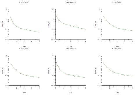
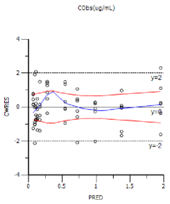
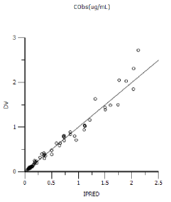
The final model appeared to fit well based on the diagnostic plots (see Figures S7, S8, S9 in Online Resource 1). The model coefficients and shrinkage estimates are shown in Tables S5 and S6 in Online Resource 1.

The LRT favored the two compartment model (with no random effects) over the corresponding one compartment model ($p<0.0001$). The $\text{CrV}_{y}$ statistic was in agreement with the LRT, having a value of 0.1419 (SE 0.03393) for the one compartment model, and 0.0428 (SE 0.01355) for the two compartment model. The $\text{CrV}_{y}$ statistic in the model with random effects also favored the full (two compartment) model over the base (one compartment) model. The value of $\text{CrV}_{y}$ for the full model was 0.01679 (SE 0.004194) and 0.1406 (SE 0.03358) for the base model.

3.3 Theophylline Example

The final model appeared to fit well based on the diagnostic plots (see Figures S10, S11, S12 in Online Resource 1). The model coefficients and shrinkage estimates are shown in Tables S7 and S8 in Online Resource 1.

The LRT favored the Tlag model ($p<0.0001$). The $\text{CrV}_{y}$ statistic was in agreement with the LRT, having a value of 0.2546 (SE 0.05727) for the model with Tlag, and 0.3927 (SE 0.10001) for the model without Tlag. The LRT had a borderline result ($p=0.0667$) for comparing the model with a body weight effect on $Ka$ and Tlag to the model without a body weight effect on $Ka$ and Tlag, while the $\eta$ versus covariate plot (Fig 3) indicated an effect. The $\text{CrV}_{\eta}$ statistic clearly favored the full model with a Tlag and a weight effect on $Ka$, having a value of 0.06220 (SE 0.02942) for the full (Tlag and wt) model, and 0.7819 (SE 0.2846) for the base (Tlag) model.

4 Discussion

As noted earlier, cross-validation is not frequently used for comparing NLME models (Brendel et al, 2007). Other methods, such as the LRT, AIC, and BIC are more commonly used. However, each of these alternative approaches have certain drawbacks. All three methods can only be applied to models having the same residual error model. The LRT can only be applied when models are nested and both models have the same random effects. Moreover, there may be an inflated type I error rate associated with the LRTs (Bertrand et al, 2009). Both the AIC and BIC have other shortcomings as well. Specifically, the AIC tends to overfit, meaning that it keeps too many covariates in the model. The BIC, in contrast, tends to underfit (fail to include significant covariates), particularly when the same size is small (Hastie et al, 2008).

Our results show that cross-validation can be used for model selection in NLME modeling and that it can produce significantly better results than these competing methods. The $\text{CrV}_{\eta}$ statistic identified the correct model at least 92.5% of the time in each of the simulated examples we considered. In contrast, the AIC was significantly more likely to select a covariate for age in our first simulation scenario (even though age had no effect on clearance in the simulated model), and both the AIC and BIC were significantly less likely to detect the effect of hepatic impairment in our fourth simulation scenario.

All four applicable methods (AIC, BIC, $\text{CrV}_{y}$, and $\text{wtCrV}_{y}$) correctly identified the true (two compartment) in our fifth simulation scenario in 100 out of 100 cases. This finding is of interest because the standard likelihood ratio test cannot be applied when there are random effects in the full model that are not present in the base model.

Both the $\text{CrV}_{y}$ statistic and the LRT favored a two compartment model in the indomethacin example. However, in the theophylline example, the population covariate plots ($\eta$’s versus covariates) seemed to suggest a weight covariate should be included in the model even though the LRT was not significant at the $p<0.05$ level. The $\text{CrV}_{\eta}$ statistic clearly favored the model with the weight covariate. This is consistent with previous studies showing that theophylline distributes poorly into body fat. Hence, the administered mg/kg dose should be calculated on the basis of ideal body weight, (Gal et al, 1978; Rohrbaugh et al, 1982) implying that body weight affects the extent of absorption. This is possible evidence that the LRT cannot always identify covariate effects when they exist and that cross-validation may be able to detect covariate effects in these situations.

Although it may seem reasonable to use the $\text{CrV}_{y}$ or $\text{wtCrV}_{y}$ statistics to determine if a covariate should be included in a model, our simulations suggest that they can give misleading results. Both statistics consistently favored models without a covariate even when a covariate effect existed. The predicted values are just as accurate with and without the covariate effect when the true model has a covariate effect, because the $\eta$’s can compensate for a missing covariate in a parameter. This suggests that one should use $\text{CrV}_{\eta}$ rather than $\text{CrV}_{y}$ or $\text{wtCrV}_{y}$ in situations when one wishes to compare different covariate models. This also indicates that it may be misleading to use cross-validation for model validation (as opposed to model selection) if one uses post hoc estimates of the $\eta$’s when calculating the predicted value of the response on the “left out” portion of the data. One may obtain a low cross-validation error rate even when the model is misspecified.

One possible drawback to using cross-validation for model selection is the fact that it is more computationally intensive than the LRT, AIC, or BIC. Leave-one-out cross-validation was applied in each of the examples in the present study, since each example consisted of relatively small data sets. However, larger data sets may require 1-2 hours (or as many as 10 hours in extreme cases), to fit a single model. If such a data set included hundreds of subjects, leave-one-out cross-validation would clearly be computationally intractible. In such situations, one may reduce the computing time by reducing the number of cross-validation folds. If 10-fold cross-validation is performed, this requires that the model be fitted only 10 times, and the number of folds could be reduced further if needed. Even a complicated model that required ten hours to fit could be evaluated over the course of several days using 5-fold cross-validation. Indeed, these cross-validation methods are no more computationally intensive than bootstrapping, which is commonly used to validate NLME models. The extra computational cost may be worthwhile in situations where it is important that the model is specified correctly.

Another potential issue with cross-validation is the fact that estimation methods for NLME models sometimes fail to converge. Although this was not a major issue in the examples we considered, if the model fails to converge for a significant proportion of the cross-validation folds, it is possible that it will produce inaccurate results. Further research is needed on the effects of lack of convergence on our proposed cross-validation methods.

These methods might be applied more generally with modifications to other types of linear mixed effects models or generalized linear mixed effects models. These methods may be applied without modification to population PK/PD models and sparser data. These are areas for future research. We expect in the sparse data case that the effectiveness of the covariate selection method may be compromised by $\eta$ shrinkage, which could distort the $\eta$ size criterion. The covariate selection method introduced in this paper may not produce correct results for parameters with high $\eta$ shrinkage (greater than 0.3, for example, in a model where the covariate is not included). The random effects for those parameters are typically removed during model development, and hence covariate adjustments may not be needed for those parameters. However, cross-validation produced correct results in our first simulation scenario even though the median shrinkage was approximately 0.3 in the base model (Figure S6 in Online Resource 1). The conditions under which our proposed cross-validation method produces valid results in sparse data sets is another area for future research.

Article Title: Cross-Validation for Nonlinear Mixed Effects Models
Journal Name: Journal of Pharmacokinetics and Pharmacodynamics

Emily Colby
Pharsight - A Certara Company
Cary, NC
and Dept. of Biostatistics
Univ. of North Carolina-Chapel Hill
Chapel Hill, NC
emily.colby@certara.com

Eric Bair
Depts. of Endodontics and Biostatistics
Univ. of North Carolina-Chapel Hill
Chapel Hill, NC
ebair@email.unc.edu

S1 Simulation Details

S1.1 Notation

In the subsequent examples, we denote the following population PK parameters with the following symbols:

• $C$: concentration of the drug in central compartment

• $C2$: concentration of the drug in peripheral compartment

• CObs: observed concentration of the drug (which is measured with error)

• $C_{\epsilon}$: error associated with CObs

• $Aa$: amount of the drug in the absorption compartment

• $A1$: amount of the drug in the central compartment

• $A2$: amount of the drug in the peripheral compartment

• $Ka$: absorption rate parameter

• $V$: systemic volume parameter

• $V2$: volume of peripheral compartment parameter

• $Cl$: systemic clearance parameter

• $Cl2$: clearance of distribution parameter

When any of the parameters above is preceded by $tv$ (i.e. $tvKa$), this represents a fixed effect (which is fixed for a given simulation but may vary across the replicates of the simulated data sets), and when a variable is preceded by $\eta$ (i.e. $\eta Ka$), this represents a random effect (which varies from subject to subject within a given simulated data set).

S1.2 Simulation Example 1: No Covariate Effects

A one-compartment, extravascular model was simulated with eight subjects using Pharsight’s Trial Simulator software (version 2.2.1). The equations for the model are as follows:

$$\frac{dAa}{dt} =-Ka\cdot Aa$$

$$\frac{dA1}{dt} =Ka\cdot Aa-Cl\cdot C$$

$$C =\frac{A1}{V}$$

A 10 percent constant CV percentage was simulated for the residual error:

$$\text{CObs}=C(1+C_{\epsilon})$$

where $\operatorname{Var}(C_{\epsilon})=0.01$.

The absorption rate parameter, $Ka$, was simulated with only a fixed effect. All other parameters were simulated with fixed and random effects as follows:

$$\begin{array}[]{rl}Ka&=tvKa\\ V&=tvV\cdot\exp(\eta V)\\ Cl&=tvCl\cdot\exp(\eta Cl)\\ \end{array}$$

The fixed effects for the PK parameters were assumed to be normally distributed at the study level (varying across replicates) with means listed below and standard deviations of 0.1:

$$\begin{array}[]{rl}\operatorname{mean}(tvKa)&=0.35\\ \operatorname{mean}(tvV)&=13.5\\ \operatorname{mean}(tvCl)&=7.4\\ \end{array}$$

The random effects ($\eta V$ and $\eta Cl$) were simulated to be independent and normally distributed at the subject level (varying across subjects) with means of 0 and variances of 0.01.

A covariate “GENDER” was simulated, so that there were 50 percent males and 50 percent females. A covariate “BODYWEIGHT” was simulated with a mean of 70 kg for males, 65 kg for females and a standard deviation of 15 for both groups. A covariate “Age” was simulated, with a mean of 40 years and a standard deviation of 10. None of the covariates had any association with the parameters, so the true underlying model had no covariate effects.

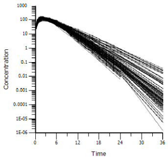
A dose of 5617 was administered at time 0 as an extravascular dose. Two hundred replicates were simulated. See Figure S1 for a plot of the simulated data.

Figure S1: Data simulated from a one compartment model with no covariate effects

Pharsight’s Phoenix NLME software (version 1.3) was used to fit two models to the simulated data. The base model was a one compartment extravascular model with random effects for $V$ and $Cl$ and no age effect on clearance. The full model was a one compartment extravascular model with random effects for $V$ and $Cl$ and an age effect on clearance. The models are specified below.

Base (correct) model:

$$\begin{array}[]{rl}Ka&=tvKa\\ V&=tvV\cdot\exp(\eta V)\\ Cl&=tvCl\cdot\exp(\eta Cl)\\ \end{array}$$

Full (incorrect) model

$$\begin{array}[]{rl}Ka&=tvKa\\ V&=tvV\cdot\exp(\eta V)\\ Cl&=tvCl\cdot(\text{Age}/40)^{dCld\text{Age}}\cdot\exp(\eta Cl)\\ \end{array}$$

where $tvKa$, $tvV$, $tvCl$, and $dCld\text{Age}$ are fixed effect parameters to be estimated. Initial estimates for the fixed effect PK parameters ($tvKa$, $tvV$, and $tvCl$) were set to the true (simulated) parameter values. The initial estimate for the covariate effect ($dCld\text{Age}$) was set to -3. The initial estimates of the variances of the random effects were all 0.1, close to the true value of 0.01.

S1.3 Simulation Example 2: Covariate Effect

A one-compartment, extravascular model was simulated with eight subjects using Pharsight’s Trial Simulator software (version 2.2.1). The equations for the model are as follows:

$$\frac{dAa}{dt} =-Ka\cdot Aa$$

$$\frac{dA1}{dt} =Ka\cdot Aa-Cl\cdot C$$

$$C =\frac{A1}{V}$$

A 10 percent constant CV percentage was simulated for the residual error:

$$\text{CObs}=C(1+C_{\epsilon})$$

where $\operatorname{Var}(C_{\epsilon})=0.01$. A fixed effect was added to the absorption rate parameter, $Ka$. All other parameters were simulated with fixed and random effects. The systemic clearance was simulated with an age effect.

$$\begin{array}[]{rl}Ka&=tvKa\\ V&=tvV\cdot\exp(\eta V)\\ Cl&=tvCl\cdot(\text{Age}/40)^{dCld\text{Age}}\cdot\exp(\eta Cl)\\ \end{array}$$

The fixed effects ($tvKa$, $tvV$, $tvCl$, and $dCld\text{Age}$) were assumed to be normally distributed at the study level (varying across replicates) with means listed below and standard deviations of 0.05, 0.1, 0.05, and 0.04, respectively.

$$\begin{array}[]{rl}\operatorname{mean}(tvKa)&=0.35\\ \operatorname{mean}(tvV)&=13.5\\ \operatorname{mean}(tvCl)&=1.2\\ \operatorname{mean}(dCld\text{Age})&=-0.9\\ \end{array}$$

The random effects ($\eta V$ and $\eta Cl$) were simulated to be independent and normally distributed at the subject level (varying across subjects) with means of 0 and variances of 0.01.

A covariate “GENDER” was simulated, so that there were 50 percent males and 50 percent females. A covariate “BODYWEIGHT” was simulated with a mean of 70 kg for males, 65 kg for females and a standard deviation of 15 for both groups. A covariate “Age” was simulated, with a mean of 40 years and a standard deviation of 10. The true underlying model had a covariate effect, namely an age effect on clearance (see below)

A dose of 5617 was administered at time 0 as an extravascular dose. Two hundred replicates were simulated. See Figure S2 for a plot of the simulated data, with clearance decreasing with age.

Figure S2: Data simulated from one a compartment model with age effect on clearance, by quartiles of age

Pharsight’s Phoenix NLME software (version 1.3) was used to fit two models to the simulated data. The base model was a one compartment extravascular model with random effects on $V$ and $Cl$ and no age effect on clearance. The full model was similar to the base model, but with an age effect included for $Cl$. The models are specified below.

Base (incorrect) model:

$$\begin{array}[]{rl}Ka&=tvKa\\ V&=tvV\cdot\exp(\eta V)\\ Cl&=tvCl\cdot\exp(\eta Cl)\\ \end{array}$$

Full (correct) model

$$\begin{array}[]{rl}Ka&=tvKa\\ V&=tvV\cdot\exp(\eta V)\\ Cl&=tvCl\cdot(\text{Age}/40)^{dCld\text{Age}}\cdot\exp(\eta Cl)\\ \end{array}$$

where $tvKa$, $tvV$, $tvCl$, and $dCld\text{Age}$ are fixed effects parameters to be estimated. Initial estimates for the fixed effects parameters ($tvKa$, $tvV$, $tvCl$, and $dCld\text{Age}$) were set to the true (simulated) parameter values. The initial estimates of the variances of the random effects were all 0.1, close to the true values of 0.01.

S1.4 Simulation Example 3: Covariate Effect in Two Compartment Model

A two-compartment, extravascular model was simulated with eight subjects using Pharsight’s Trial Simulator software (version 2.2.1). The equations for the model are as follows:

$$\frac{dAa}{dt} =-Ka\cdot Aa$$

$$\frac{dA1}{dt} =Ka\cdot Aa-Cl\cdot C-Cl2\cdot(C-C2)$$

$$\frac{dA2}{dt} =Cl2\cdot(C-C2)$$

$$C =\frac{A1}{V}$$

$$C2 =\frac{A2}{V2}$$

A 10 percent constant CV percentage was simulated for the residual error:

$$\text{CObs}=C(1+C_{\epsilon})$$

where $\operatorname{Var}(C_{\epsilon})=0.01$.

A fixed effect was added to the absorption rate parameter, $Ka$. All other parameters were simulated with fixed and random effects. The systemic clearance was simulated with an age effect.

$$\begin{array}[]{rl}Ka&=tvKa\\ V&=tvV\cdot\exp(\eta V)\\ V2&=tvV2\cdot\exp(\eta V2)\\ Cl&=tvCl\cdot(\text{Age}/40)^{dCld\text{Age}}\cdot\exp(\eta Cl)\\ Cl2&=tvCl2\cdot\exp(\eta Cl2)\\ \end{array}$$

The fixed effects ($tvKa$, $tvV$, $tvV2$, $tvCl$, $tvCl2$, and $dCld\text{Age}$) were assumed to be normally distributed at the study level (varying across replicates) with means listed below and standard deviations of 0.05, 0.1, 0.1, 0.05, 0.05, and 0.04, respectively.

$$\begin{array}[]{rl}\operatorname{mean}(tvKa)&=0.35\\ \operatorname{mean}(tvV)&=13.5\\ \operatorname{mean}(tvV2)&=36\\ \operatorname{mean}(tvCl)&=1.2\\ \operatorname{mean}(tvCl2)&=0.62\\ \operatorname{mean}(dCld\text{Age})&=-0.9\\ \end{array}$$

The random effects ($\eta V$, $\eta V2$, $\eta Cl$, and $\eta Cl2$) were simulated to be independent and normally distributed at the subject level (varying across subjects) with means of 0 and variances of 0.01.

A covariate “GENDER” was simulated, so that there were 50 percent males and 50 percent females. A covariate “BODYWEIGHT” was simulated with a mean of 70 kg for males, 65 kg for females and a standard deviation of 15 for both groups. A covariate “Age” was simulated, with a mean of 40 years and a standard deviation of 10. The true underlying model had a covariate effect, namely an age effect on clearance (see below).

A dose of 5617 was administered at time 0 as an extravascular dose. Two hundred replicates were simulated. See Figure S3 for a plot of the simulated data, with clearance decreasing with age.

Figure S3: Data simulated from a two compartment model with age effect on clearance, by quartiles of age

Pharsight’s Phoenix NLME software (version 1.3) was used to fit two models to the simulated data. The base model was a two compartment extravascular model with random effects on $V$, $V2$, $Cl$, and $Cl2$ and no age effect on clearance. The full model was similar to the base model, but with an age effect included for $Cl$. The models are specified below.

Base (incorrect) model:

$$\begin{array}[]{rl}Ka&=tvKa\\ V&=tvV\cdot\exp(\eta V)\\ V2&=tvV2\cdot\exp(\eta V2)\\ Cl&=tvCl\cdot\exp(\eta Cl)\\ Cl2&=tvCl2\cdot\exp(\eta Cl2)\\ \end{array}$$

Full (correct) model:

$$\begin{array}[]{rl}Ka&=tvKa\\ V&=tvV\cdot\exp(\eta V)\\ V2&=tvV2\cdot\exp(\eta V2)\\ Cl&=tvCl\cdot(\text{Age}/40)^{dCld\text{Age}}\cdot\exp(\eta Cl)\\ Cl2&=tvCl2\cdot\exp(\eta Cl2)\\ \end{array}$$

where $tvKa$, $tvV$, $tvV2$, $tvCl$, $tvCl2$, and $dCld\text{Age}$ are fixed effects parameters to be estimated. Initial estimates for the fixed effects parameters ($tvKa$, $tvV$, $tvV2$, $tvCl$, $tvCl2$, and $dCld\text{Age}$) were set to the true (simulated) parameter values. The initial estimates of the variances of the random effects were all 0.1, close to the true values of 0.01.

S1.5 Simulation Example 4: Five Covariate Effects

A one compartment, extravascular model was simulated with eight subjects using Pharsight’s Trial Simulator software (version 2.2.1). The equations for the model are as follows:

$$\frac{dAa}{dt} =-Ka\cdot Aa$$

$$\frac{dA1}{dt} =Ka\cdot Aa-Cl\cdot C$$

$$C =\frac{A1}{V}$$

A 10 percent constant CV percentage was simulated for the residual error:

$$\text{CObs}=C(1+C_{\epsilon})$$

where $\operatorname{Var}(C_{\epsilon})=0.01$.

A fixed effect was added to the absorption rate parameter, $Ka$. All other parameters were simulated with fixed and random effects. The systemic volume was simulated with a body weight effect. The systemic clearance was simulated with body weight (BW), age (Age), gender (Gender), and hepatic impairment (HI) effects:

$$\begin{array}[]{rl}Ka&=tvKa\\ V&=tvV\cdot(\text{BW}/70)^{dVd\text{BW}}\cdot\exp(\eta V)\\ Cl&=tvCl\cdot(\text{BW}/70)^{dCld\text{BW}}\cdot(\text{Age}/40)^{dCld\text{Age}}\cdot(1+dCld\text{Gender})\\ &\cdot(1+dCld\text{HI}*\text{HI})\cdot\exp(\eta Cl)\\ \end{array}$$

The fixed effects ($tvKa$, $tvV$, $tvCl$, $dVd\text{BW}$, $dCld\text{BW}$, $dCld\text{Age}$, $dCld\text{Gender}$, and $dCld\text{HI}$) were assumed to be normally distributed at the study level (varying across replicates) with means listed below and standard deviations of 0.05, 0.1, 0.05, 0.1, 0.1, 0.04, 0.05, and 0.05 respectively.

$$\begin{array}[]{rl}\operatorname{mean}(tvKa)&=0.35\\ \operatorname{mean}(tvV)&=13.5\\ \operatorname{mean}(tvCl)&=1.2\\ \operatorname{mean}(dVd\text{BW})&=1\\ \operatorname{mean}(dCld\text{BW})&=0.75\\ \operatorname{mean}(dCld\text{Age})&=-0.9\\ \operatorname{mean}(dCld\text{Gender})&=0.1\\ \operatorname{mean}(dCld\text{HI})&=-0.2\\ \end{array}$$

The random effects ($\eta V$ and $\eta Cl$) were simulated to be independent and normally distributed at the subject level (varying across subjects) with means of 0 and variances of 0.01.

A covariate “Gender” was simulated, so that there were 50 percent males (Gender=1) and 50 percent females (Gender=0). A covariate for body weight “BW” was simulated with a mean of 70 kg for males, 65 kg for females and a standard deviation of 15 for both groups. A covariate “Age” was simulated, with a mean of 40 years and a standard deviation of 10. A covariate for hepatic impairment “HI” was simulated, with 70 percent not hepatically impaired (HI=0) and 30 percent hepatically impaired (HI=1). The true underlying model had five covariate effects, namely a body weight effect on volume, and age, body weight, gender, and hepatic impairment effects on clearance (see below).

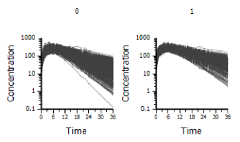
A dose of 5617 was administered at time 0 as an extravascular dose. Two hundred replicates were simulated. See Figure S4 for a plot of the simulated data.

Figure S4: Data simulated from a one compartment model with body weight effect on volume, and body weight, gender, age, and hepatic impairment effects on clearance, by hepatic impairment (0=Not hepatically impaired, 1=Hepatically impaired)

Pharsight’s Phoenix NLME software (version 1.3) was used to fit two models to the simulated data. The base model was a one compartment extravascular model with random effects on $V$ and $Cl$, a body weight effect on $V$, and age, gender, and body weight effects on $Cl$. The full model was similar to the base model, but with a hepatic impairment effect also included for $Cl$. The models are specified below.

Base (incorrect) model:

$$\begin{array}[]{rl}Ka&=tvKa\\ V&=tvV\cdot(\text{BW}/70)^{dVd\text{BW}}\cdot\exp(\eta V)\\ Cl&=tvCl\cdot(\text{BW}/70)^{dCld\text{BW}}\cdot(\text{Age}/40)^{dCld\text{Age}}\cdot(1+dCld\text{Gender})\cdot\exp(\eta Cl)\\ \end{array}$$

Full (correct) model:

$$\begin{array}[]{rl}Ka&=tvKa\\ V&=tvV\cdot(\text{BW}/70)^{dVd\text{BW}}\cdot\exp(\eta V)\\ Cl&=tvCl\cdot(\text{BW}/70)^{dCld\text{BW}}\cdot(\text{Age}/40)^{dCld\text{Age}}\cdot(1+dCld\text{Gender})\\ &\cdot(1+dCld\text{HI}*\text{HI})\cdot\exp(\eta Cl)\\ \end{array}$$

where $tvKa$, $tvV$, $tvCl$, $dVd\text{BW}$, $dCld\text{BW}$, $dCld\text{Age}$, $dCld\text{Gender}$, and $dCld\text{HI}$ are fixed effects parameters to be estimated. Initial estimates for the fixed effects parameters were set to the true (simulated) parameter values. The initial estimates of the variances of the random effects were all 0.1, close to the true values of 0.01.

S1.6 Simulation Example 5: Two compartment model

A two compartment, extravascular model was simulated with six subjects using Pharsight’s Trial Simulator software (version 2.2.1). The equations for the model are as follows:

$$\frac{dAa}{dt} =-Ka\cdot Aa$$

$$\frac{dA1}{dt} =Ka\cdot Aa-Cl\cdot C-Cl2\cdot(C-C2)$$

$$\frac{dA2}{dt} =Cl2\cdot(C-C2)$$

$$C =\frac{A1}{V}$$

$$C2 =\frac{A2}{V2}$$

A 10 percent constant CV percentage was simulated for the residual error:

$$\text{CObs}=C(1+C_{\epsilon})$$

where $\operatorname{Var}(C_{\epsilon})=0.01$.

A fixed effect was added to the absorption rate parameter, $Ka$. All other parameters were simulated with fixed and random effects:

$$\begin{array}[]{rl}Ka&=tvKa\\ V&=tvV\cdot\exp(\eta V)\\ V2&=tvV2\cdot\exp(\eta V2)\\ Cl&=tvCl\cdot\exp(\eta Cl)\\ Cl2&=tvCl2\cdot\exp(\eta Cl2)\\ \end{array}$$

The fixed effects for the PK parameters were assumed to be normally distributed at the study level (varying across replicates) with means listed below and standard deviations of 0.1, except in this example the fixed effect for $Ka$ was simulated with a standard deviation of 0.05 because when the absorption rate was smaller the portion of the curve for the first compartment became less pronounced in relation to the portion for the second compartment. Having a smaller standard deviation for $Ka$ increased the chance that all the simulated profiles would have a characteristic two compartment shape.

$$\begin{array}[]{rl}\operatorname{mean}(tvKa)&=0.35\\ \operatorname{mean}(tvV)&=13.5\\ \operatorname{mean}(tvV2)&=34\\ \operatorname{mean}(tvCl)&=7.4\\ \operatorname{mean}(tvCl2)&=1.2\\ \end{array}$$

The random effects ($\eta V$, $\eta V2$, $\eta Cl$, and $\eta Cl2$) were simulated to be normally distributed at the subject level (varying across subjects) with means of 0 and variances of 0.01.

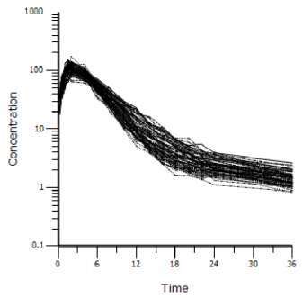
A dose of 5617 was administered at time 0 as an extravascular dose. One hundred replicates were simulated. See Figure S5 for a plot of the simulated data.

Figure S5: Data simulated from a two compartment model with no covariate effects

Pharsight’s Phoenix NLME software (version 1.3) was used to fit a base model with one compartment and a full model with two compartments to the simulated data. The models are specified below.

Base (incorrect) model

$$\begin{array}[]{rl}Ka&=tvKa\\ V&=tvV\cdot\exp(\eta V)\\ Cl&=tvCl\cdot\exp(\eta Cl)\\ \end{array}$$

Full (correct) model

$$\begin{array}[]{rl}Ka&=tvKa\\ V&=tvV\cdot\exp(\eta V)\\ V2&=tvV2\cdot\exp(\eta V2)\\ Cl&=tvCl\cdot\exp(\eta Cl)\\ Cl2&=tvCl2\cdot\exp(\eta Cl2)\\ \end{array}$$

where $tvKa$, $tvV$, $tvV2$, $tvCl$, and $tvCl2$ are fixed effects parameters to be estimated. Initial estimates for the fixed effects parameters ($tvKa$, $tvV$, $tvV2$, $tvCl$, and $tvCl2$) were set to the true (simulated) parameter values. The initial estimates of the variances of the random effects were all 0.1, close to the true values of 0.01.

S2 Distribution of the Selection Statistics and Shrinkage in the Simulated Data Sets

For each simulated data set, the values of AIC, BIC, $\text{CrV}_{\eta}$, $\text{CrV}_{y}$, and $\text{wtCrV}_{y}$ were calculated, along with the standard error of each statistic. Tables S1, S2, S3, and S4 show the mean values and standard deviations of both the statistics and the standard errors over 200 simulations (or 100 simulations in the case of scenario 5). Furthermore, boxplots of the $\eta$ shrinkage values for each model under scenarios 1-4 are shown in Figure S6.

Table S1: Distribution of AIC and BIC in each simulation scenario

				AIC		BIC
Scen.	Base Model	Full Model		Base	Full	Base	Full
1	✓1 Cpt	1 Cpt,	N	200	200	200	200
		Age-Cl	Mean	384	404	401	424
			SD	114	115	114	115
2	1 Cpt	✓1 Cpt,	N	200	200	200	200
		Age-Cl	Mean	1106	1093	1124	1113
			SD	25	25	25	25
3	2 Cpt	✓2 Cpt,	N	200	200	200	200
		Age-Cl	Mean	1039	1026	1068	1058
			SD	27	27	29	29
4	1 Cpt, BW-V;	✓1 Cpt, BW-V;	N	200	200	200	200
	BW-Cl, G-Cl,	BW-Cl, G-Cl,	Mean	1106	1100	1135	1132
	Age-Cl	Age-Cl, HI-Cl	SD	33	32	33	32
5	1 Cpt	✓2 Cpt	N	100	100	100	100
			Mean	648	417	664	443
			SD	218	26	218	26

✓indicates true model, Cpt=Compartment, Age-Cl indicates age effect on clearance, BW=Body Weight, V=Volume, G=Gender, HI=Hepatic Impairment

Table S2: Distribution of $\text{CrV}_{\eta}$ in each simulation scenario

				$\text{CrV}_{\eta}$		SE($\text{CrV}_{\eta}$)
Scen.	Base Model	Full Model		Base	Full	Base	Full
1	✓1 Cpt	1 Cpt,	N	200	200	200	200
		Age-Cl	Mean	0.136	0.919	0.022	0.403
			SD	0.236	0.920	0.032	0.512
2	1 Cpt,	✓1 Cpt,	N	200	200	200	200
		Age-Cl	Mean	0.078	0.012	0.031	0.005
			SD	0.056	0.010	0.022	0.005
3	2 Cpt	✓2 Cpt,	N	200	200	200	200
		Age-Cl	Mean	0.144	0.024	0.077	0.020
			SD	0.728	0.155	0.453	0.155
4	1 Cpt, BW-V;	✓1 Cpt, BW-V;	N	200	200	200	200
	BW-Cl, G-Cl,	BW-Cl, G-Cl,	Mean	1.700	0.124	0.626	0.081
	Age-Cl	Age-Cl, HI-Cl	SD	2.577	0.281	2.515	0.214

✓indicates true model, Cpt=Compartment, Age-Cl indicates age effect on clearance, BW=Body Weight, V=Volume, G=Gender, HI=Hepatic Impairment

Table S3: Distribution of $\text{CrV}_{y}$ in each simulation scenario

				$\text{CrV}_{y}$		SE($\text{CrV}_{y}$)
Scen.	Base Model	Full Model		Base	Full	Base	Full
1	✓1 Cpt	1 Cpt,	N	200	200	200	200
		Age-Cl	Mean	41.1	46.4	13.3	18.5
			SD	58.4	82.0	51.6	73.6
2	1 Cpt	✓1 Cpt,	N	200	200	200	200
		Age-Cl	Mean	247	254	45.6	47.2
			SD	54.0	59.0	24.4	25.5
3	2 Cpt	✓2 Cpt,	N	200	200	200	200
		Age-Cl	Mean	159	199	28.0	59.9
			SD	34.9	171	12.5	160
4	1 Cpt, BW-V;	✓1 Cpt, BW-V;	N	200	200	200	200
	BW-Cl, G-Cl,	BW-Cl, G-Cl,	Mean	323	472	85.1	173
	Age-Cl	Age-Cl, HI-Cl	SD	116	401	72.2	284
5	1 Cpt	✓2 Cpt	N	100	100	100	100
			Mean	206.11	30.28	32.32	8.32
			SD	90.3	9.60	20.7	5.74

✓indicates true model, Cpt=Compartment, Age-Cl indicates age effect on clearance, BW=Body Weight, V=Volume, G=Gender, HI=Hepatic Impairment

Table S4: Distribution of $\text{wtCrV}_{y}$ in each simulation scenario

				$\text{wtCrV}_{y}$		SE($\text{wtCrV}_{y}$)
Scen.	Base Model	Full Model		Base	Full	Base	Full
1	✓1 Cpt	1 Cpt,	N	200	200	200	200
		Age-Cl	Mean	1.14	1.20	0.157	0.176
			SD	0.303	0.388	0.064	0.154
2	1 Cpt	✓1 Cpt,	N	200	200	200	200
		Age-Cl	Mean	0.967	1.01	0.144	0.154
			SD	0.133	0.130	0.120	0.111
3	2 Cpt	✓2 Cpt,	N	200	200	200	200
		Age-Cl	Mean	1.0096	1550*	0.154	1550*
			SD	0.0995	21700*	0.071	21700*
4	1 Cpt, BW-V;	✓1 Cpt, BW-V;	N	200	200	200	200
	BW-Cl, G-Cl,	BW-Cl, G-Cl,	Mean	1.25	2.78	0.305	1.56
	Age-Cl	Age-Cl, HI-Cl	SD	0.485	11.6	0.432	11.3
5	1 Cpt	✓2 Cpt	N	100	100	100	100
			Mean	14.7	1.14	3.09	0.233
			SD	10.1	0.143	2.86	0.130

✓indicates true model, Cpt=Compartment, Age-Cl indicates age effect on clearance, BW=Body Weight, V=Volume, G=Gender, HI=Hepatic Impairment
*One of the replicates (161) had an inflated value for $\text{wtCrV}_{y}$. One subject was significantly younger than the others, and the effect of age on clearance was estimated to be around -22 instead of the true value of -0.9 in the model where this subject was left out. Hence the younger subject had inflated residuals.

Figure S6: Boxplots of the $\eta$ shrinkage values for each model under scenarios 1-4

S3 Additional Details for the Indomethacin Data Example

S3.1 Model for the Indomethacin Data Analysis

In this analysis, we compared the following two compartment IV bolus model

$$\frac{dA1}{dt} =-Cl\cdot C-Cl2\cdot(C-C2)$$

$$\frac{dA2}{dt} =Cl2\cdot(C-C2)$$

$$C =\frac{A1}{V}$$

$$C2 =\frac{A2}{V2}$$

to the corresponding one compartment model:

$$\frac{dA1}{dt} =-Cl\cdot C$$

$$C =\frac{A1}{V}$$

In the above equations, we use the same notation that was defined in Section S1.1. A constant CV percentage was modeled for the residual error in both cases:

$$\text{CObs}=C(1+C_{\epsilon})$$

Under the full (two compartment) model, all PK parameters were modeled with fixed and random effects:

$$\begin{array}[]{rl}V&=tvV\cdot\exp(\eta V)\\ V2&=tvV2\cdot\exp(\eta V2)\\ Cl&=tvCl\cdot\exp(\eta Cl)\\ Cl2&=tvCl2\cdot\exp(\eta Cl2)\end{array}$$

where $tvKa$, $tvV$, $tvV2$, $tvCl$, and $tvCl2$ are fixed effects parameters to be estimated. The corresponding base (one compartment) model was similar:

$$\begin{array}[]{rl}V&=tvV\cdot\exp(\eta V)\\ Cl&=tvCl\cdot\exp(\eta Cl)\end{array}$$

The fixed effects for the PK parameters were set to the following initial values.

$$\begin{array}[]{rl}tvV&=7551\\ tvV2&=13531\\ tvCl&=8368\\ tvCl2&=7056\\ \end{array}$$

The random effects ($\eta V$, $\eta V2$, $\eta Cl$, and $\eta Cl2$) were set to have initial variances of 1.

S3.2 Parameter Estimates and Diagnostic Plots for the Indomethacin Data Analysis

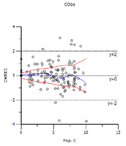
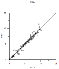
The coefficient estimates for the fixed effects of the indomethacin model are shown in Table S5, and the estimated variance-covariance matrix is shown in Table S6. To assess the model fit, three diagnostic plots were created. Figure S7 shows the predicted and observed concentrations over time for all six subjects in the data set. Figure S8 shows a plot of the conditional weighted residuals versus the predicted concentrations. Figure S9 shows a scatter plot of the observed concentrations versus the predicted concentrations. In each case, no obvious problems are visible, suggesting that the model fit is adequate.

Table S5: Parameter estimates for the indomethacin model

Parameter	Estimate	Units	Stderr	Stderr%
$tvV$	8898	mL	574.84	6.46
$tvV2$	19527.3	mL	3169.70	16.23
$tvCl$	7905.99	mL/h	608.53	7.70
$tvCl2$	5252.15	mL/h	768.93	14.64
$\sigma$	0.1440		0.02	13.25

$\sigma$ denotes the estimated residual standard deviation
prefix of ’tv’ denotes fixed effect or typical value

Table S6: Estimated variance/covariance matrix ($\Omega$) of the random effects for the indomethacin model

	$\eta V$	$\eta Cl$	$\eta V2$	$\eta Cl2$
$\eta V$	0.0017
$\eta Cl$	0	0.0338
$\eta V2$	0	0	0.0666
$\eta Cl2$	0	0	0	0.1202
Shrinkage	0.7064	0.0329	0.3321	0.0727

Figure S7: Predicted (lines) and observed (dots) concentrations versus time for the indomethacin model

Figure S8: Conditional weighted residuals versus predicted values for the indomethacin model

Figure S9: Observed versus individual predicted values for the indomethacin model

S4 Additional Details for the Theophylline Data Example

S4.1 Model for the Theophylline Data Analysis

A one compartment extravascular model with clearance parametrization was fit to this data set. The equations for the model are as follows:

$$\frac{dAa}{dt} =-Ka\cdot Aa$$

$$\frac{dA1}{dt} =Ka\cdot Aa-Cl\cdot C$$

$$C =\frac{A1}{V}$$

In the above equations, we use the same notation that was defined in Section S1.1. The dose to the absorption compartment is delayed by a parameter Tlag. An additive weighting scheme was modeled for the residual error:

$$\text{CObs}=C+C_{\epsilon}$$

A fixed effect was added to the time lag parameter, Tlag. All other parameters were modeled with fixed and random effects:

$$\begin{array}[]{rl}Ka&=tvKa\cdot(\text{wt}/\operatorname{mean}(\text{wt}))^{dKad\text{wt}}\cdot\exp(\eta Ka)\\ V&=tvV\cdot\exp(\eta V)\\ Cl&=tvCl\cdot\exp(\eta Cl)\\ \text{Tlag}&=tv\text{Tlag}\\ \end{array}$$

where $tvKa$, $tvV$, $tvV2$, $tvCl$, and $tvCl2$ are fixed effects parameters to be estimated, and wt is the body weight of a subject in kg and $\operatorname{mean}(\text{wt})$ is the average of the body weights in the data set. This full model was compared to two base models. The first base model did not include a Tlag parameter nor a covariate for weight:

$$\begin{array}[]{rl}Ka&=tvKa\cdot\exp(\eta Ka)\\ V&=tvV\cdot\exp(\eta V)\\ Cl&=tvCl\cdot\exp(\eta Cl)\end{array}$$

The second base model included a Tlag parameter but no covariate for weight:

$$\begin{array}[]{rl}Ka&=tvKa\cdot\exp(\eta Ka)\\ V&=tvV\cdot\exp(\eta V)\\ Cl&=tvCl\cdot\exp(\eta Cl)\\ \text{Tlag}&=tv\text{Tlag}\\ \end{array}$$

The full model included a Tlag parameter and a covariate for weight:

$$\begin{array}[]{rl}Ka&=tvKa\cdot(\text{wt}/mean(\text{wt})^{dKad\text{wt}}\cdot\exp(\eta Ka)\\ V&=tvV\cdot\exp(\eta V)\\ Cl&=tvCl\cdot\exp(\eta Cl)\\ \text{Tlag}&=tv\text{Tlag}\\ \end{array}$$

The fixed effects for the PK parameters were set to the following initial values:

$$\begin{array}[]{rl}tvKa&=2\\ tvV&=1\\ tvCl&=1\\ tvTlag&=1\\ dKad\text{wt}&=0\\ \end{array}$$

The random effects ($\eta V$, $\eta Ka$, and $\eta Cl$) were set to have initial variances of 1 in a diagonal variance-covariance matrix.

S4.2 Parameter Estimates and Diagnostic Plots for the Theophylline Data Analysis

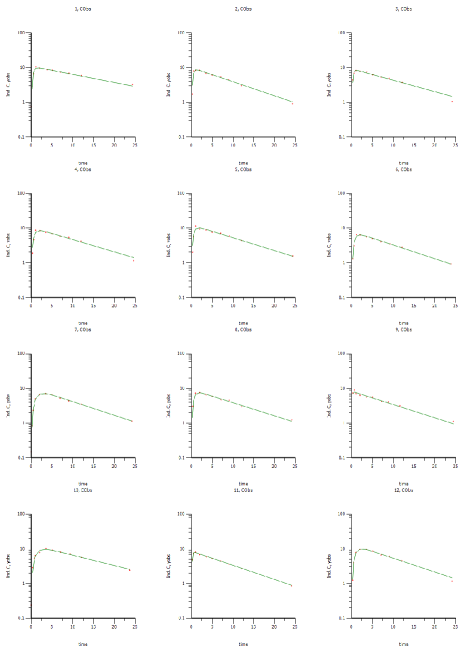
The coefficient estimates for the fixed effects of the indomethacin model are shown in Table S7, and the estimated variance-covariance matrix is shown in Table S8. To assess the model fit, three diagnostic plots were created. Figure S10 shows the predicted and observed concentrations over time for all six subjects in the data set. Figure S11 shows a plot of the conditional weighted residuals versus the predicted concentrations. Figure S12 shows a scatter plot of the observed concentrations versus the predicted concentrations. In each case, no obvious problems are visible, suggesting that the model fit is adequate.

Table S7: Parameter estimates for the final theophylline model

Parameter	Estimate	Stderr	Stderr%
$tvKa$	2.63	0.37	13.89
$tvV$	0.47	0.02	4.36
$tvCl$	0.04	0.00	8.01
$tvTlag$	0.16	0.01	9.18
$tvdKadwt$	3.07	0.76	24.81
$\sigma$	0.55	0.04	7.16

$\sigma$ denotes the estimated residual standard deviation
prefix of ’tv’ denotes fixed effect or typical value

Table S8: Estimated variance/covariance matrix ($\Omega$) of the random effects for the final theophylline model

	$\eta V$	$\eta Ka$	$\eta Cl$
$\eta V$	0.0196
$\eta Ka$	0	0.5208
$\eta Cl$	0	0	0.0698
Shrinkage	0.0728	0.0276	0.0552

Figure S10: Predicted (lines) and observed (dots) concentrations versus time for the final theophylline model

Figure S11: Conditional weighted residuals versus predicted values for the final theophylline model

Figure S12: Observed versus individual predicted values for the final theophylline model