High-order multiderivative time integrators for hyperbolic conservation laws

Abstract

Multiderivative time integrators have a long history of development for ordinary differential equations, and yet to date, only a small subset of these methods have been explored as a tool for solving partial differential equations (PDEs). This large class of time integrators include all popular (multistage) Runge-Kutta as well as single-step (multiderivative) Taylor methods. (The latter are commonly referred to as Lax-Wendroff methods when applied to PDEs.) In this work, we offer explicit multistage multiderivative time integrators for hyperbolic conservation laws. Like Lax-Wendroff methods, multiderivative integrators permit the evaluation of higher derivatives of the unknown in order to decrease the memory footprint and communication overhead. Like traditional Runge-Kutta methods, multiderivative integrators admit the addition of extra stages, which introduce extra degrees of freedom that can be used to increase the order of accuracy or modify the region of absolute stability. We describe a general framework for how these methods can be applied to two separate spatial discretizations: the discontinuous Galerkin (DG) method and the finite difference essentially non-oscillatory (FD-WENO) method. The two proposed implementations are substantially different: for DG we leverage techniques that are closely related to generalized Riemann solvers; for FD-WENO we construct higher spatial derivatives with central differences. Among multiderivative time integrators, we argue that multistage two-derivative methods have the greatest potential for multidimensional applications, because they only require the flux function and its Jacobian, which is readily available. Numerical results indicate that multiderivative methods are indeed competitive with popular strong stability preserving time integrators.

1 Introduction

In this work we revisit classical ordinary differential equation (ODE) solvers known as multiderivative (Obreshkoff Obreschkoff40 ) methods. It will be shown that this large class of time integrators include all explicit Runge-Kutta and Taylor methods as special cases. In particular, we demonstrate how a multiderivative ODE method can be used to solve hyperbolic conservation laws. We begin by presenting the definitions and notation used throughout this work.

A conservation law is a partial differential equation (PDE) defined by a flux function $R$ of the form

$$q_{,t}+\nabla_{\bf x}\cdot R(q)=0,\quad q(0,{\bf x})=q_{0}({\bf x}),\quad{\bf x}\in\Omega\subseteq\mathbb{R}^{d},$$ (1)

where the solution $q(t,{\bf x}):\mathbb{R}^{+}\times\mathbb{R}^{d}\to\mathbb{R}^{m}$ is a vector of $m$ conserved quantities. In dimension $d$, this initial value problem is defined by $m$ equations with prescribed initial conditions $q_{0}:\mathbb{R}^{d}\to\mathbb{R}^{m}$. We denote the flux function $R:\mathbb{R}^{m}\to\mathbb{R}^{d}\times\mathbb{R}^{m}$ with $R=[f^{(1)},f^{(2)},\dots,f^{(d)}]^{T}$. We say (1) is hyperbolic if the matrix

$${\bf n}^{(1)}\frac{\partial f^{(1)}}{\partial q}(q)+{\bf n}^{(2)}\frac{\partial f^{(2)}}{\partial q}(q)+\cdots{\bf n}^{(d)}\frac{\partial f^{(d)}}{\partial q}(q)$$ (2)

is diagonalizable for every ${\bf n}\in\mathbb{R}^{d}$ satisfying $\|{\bf n}\|=1$ and $q$ in the domain of interest.

Numerical methods for solving (1) require a discretization technique for space as well as a (possibly coupled) discretization technique for time. The vast majority of time stepping discretizations fall into one of two distinct categories:

• Method of lines formulation.

  A method of lines (MOL) solver for (1) separates the spatial discretization from the time evolution. Starting with $q_{,t}=-\nabla_{{\bf x}}\cdot R(q)$, one defines a spatial discretization $q^{h}$ of the continuous variable $q$, which could be tracking point values (finite difference, spectral methods), cell averages (finite volume methods), or coefficients of basis functions (finite element methods). This operation defines a function $\mathcal{L}(q^{h})=-\nabla_{{\bf x}}\cdot R(q^{h})$, that in turn defines a large ODE system of the form:

  $$q^{h}_{,t}=\mathcal{L}(q^{h}).$$ (3)

  Once this discretization has been parsed, one may apply an appropriate ODE integrator to this problem: for hyperbolic conservation laws, explicit time-stepping methods are usually preferred.

• Lax-Wendroff (Taylor) formulation.

  The Lax-Wendroff LxW60 procedure is a numerical scheme that updates the solution using finitely many terms from the Taylor series of the function. Here, one first expands $q(t,{\bf x})$ in time about $t=t^{n}$:

  $$q(t,{\bf x})=q^{n}+(t-t^{n})q^{n}_{,t}+\frac{(t-t^{n})^{2}}{2!}q^{n}_{,tt}+\cdots,$$ (4)

  and then each time derivative is replaced with a spatial derivative via the Cauchy-Kowalewski procedure:

  $$q_{,t} =-\nabla_{\bf x}\cdot R(q),$$ (5)

  $$q_{,tt} =-\nabla_{{\bf x}}\cdot R(q)_{t}=-\nabla_{{\bf x}}\cdot\left(R^{\prime}(q)q_{,t}\right)=\nabla_{{\bf x}}\cdot\left(R^{\prime}(q)\cdot\nabla_{{\bf x}}\cdot R(q)\right),$$

  $$\vdots$$

  Further derivatives are required for higher order variants, and of course, one still needs to choose a spatial discretization. Inserting $t=t^{n}+\Delta t$ produces a single-stage, single-step method. In addition, this is fundamentally different than the MOL discretization, because the physical and temporal variables are intimately intertwined through the choice of the spatial discretization of the right hand side of (4).

Multiderivative Runge-Kutta time integrators form the bridge that unifies these two disparate families of methods by defining a framework that includes each of them as special cases. We will see that the generalization presented in this work makes use of techniques used in the development of high-order method of lines formulations as well as high-order Lax-Wendroff type time discretizations.

1.1 High-order method of lines formulation for PDEs

The most popular high-order time integrators for hyperbolic problems fall into the method of lines category. By and large, the predominant viewpoint from the community is to develop spatial discretizations separate from time integrators. This is incredibly attractive from a software engineering perspective: one can envision developing a code that completely decouples the ODE technology from the spatial discretization. In addition, the MOL formulation invites developers to concentrate efforts on ODE integrators as a separate entity from the PDE. However, this idealization is lacking given that a numerical scheme is intended to solve a PDE, and therefore one needs to respect the choice of spatial discretization not only when selecting an ODE integrator, but also when developing one. In contrast, Taylor methods require a recognition of the particular choice of spatial discretization.

1.2 High-order Lax-Wendroff methods for PDEs

The Lax-Wendroff procedure is much older than either Lax or Wendroff. Indeed, a more appropriate name would be the Cauchy-Kowalewski procedure, where Cauchy and Kowalewski sought methods that could aid them in proving existence and uniqueness for solutions to PDEs. Their combined method, known as the Cauchy-Kowalewski procedure, was presented in equation (5), and is derived from Brook Taylor’s method, who invented equation (4) in the 1700’s. For a modern (mid-$20^{\text{th}}$ century) proof and review of the Cauchy-Kowalewski procedure see Friedman Friedman61 or Fusaro Fusaro68 and references therein. In 1960, Peter Lax and Burton Wendroff LxW60 realized the Cauchy-Kowalewski procedure could be used as a numerical method. They started with the theoretical groundwork developed by Cauchy and Kowalewski and derived a numerical scheme for solving PDEs. Therefore, this entire procedure is often cited as the Lax-Wendroff method within the numerical analysis community.

The original Lax-Wendroff method was a second-order numerical discretization of the Cauchy-Kowalewski procedure, and over the past decade, much work has been put forth to define high-order variants of this method. In 2002, Toro and Titarev started work on a series of papers that became the basis for the so-called ADER (Arbitrary DERivative) methods that define high-order versions of the Lax-Wendroff procedure proceedings:TitarevToro02 ; ToroTitarev02 ; ToroTitarev05:JCP ; TitarevToro05:JCP:systems ; ToroTitarev05:JSP . During that same time period, Daru and Tenaud DaruTenaud04 explored high-order monotonicity preserving single-step methods, and they derived TVD flux limiters to control spurious oscillations. In 2003, Jianxian Qiu and his collaborators demonstrated a high-order extension of the Lax-Wendroff procedure using finite difference weighted essentially non-oscillatory (WENO) methods QiuShu03 . Later on, they applied the same procedure to Hamilton-Jacobi systems as well as the shallow water equations Qiu07 ; LuQiu11 . Additionally, Qiu, Dumbser and Shu showed how to apply the Lax-Wendroff scheme to the discontinuous Galerkin (DG) method QiuDumbserShu05 , and shortly thereafter, Dumbser and Munz followed a similar procedure for constructing DG methods to arbitrarily high orders of accuracy using generalized Riemann solvers DuMu06 . High-order versions of a Lax-Wendroff discontinuous Galerkin method have been investigated for ideal magnetohydrodynamic equations TaDuBaDiMu07 , and explorations into various numerical flux functions for the Lax-Wendroff DG method has also been carried out JQiu07 . It has already been noted that high-order schemes with Lax-Wendroff type time discretizations can be implemented to carry a low-memory footprint LiuChengShu09 .

Much of the difficulty when constructing high-order versions of the Lax-Wendroff scheme comes from the necessity of defining higher spatial derivatives of the solution. After producing the Jacobian of the flux function, the next time derivative produces the Hessian of the flux function. Further derivatives require tensors which grow vastly in size, and therefore, one of the primary concerns with a high-order Lax-Wendroff method is the burden of implementing higher derivatives, especially in higher dimensions.

1.3 High-order multistage multiderivative methods for PDEs

In this work, we advocate the use of multistage multiderivative integrators for solving hyperbolic conservation laws. These time integrators are the natural generalization of MOL formulations as well as pure Taylor (Lax-Wendroff) methods. The introduction of higher derivatives allows one to design compact stencils, and the introduction of degrees of freedom to Taylor methods allows one to explore closely related alternatives. We argue that the benefits of exploring multiderivative time integrators include, but are not limited to the following:

• High-order accuracy [$3^{rd}$-order or higher]. Explicit multiderivative schemes can be constructed to arbitrarily high orders of accuracy. We focus on a single fourth-order method as our demonstrative example.

• Portability. Access to the eigen-decomposition of a hyperbolic problem is a necessity. Therefore, multistage multiderivative integrators that stop at the second derivative do not require anything above and beyond anything that is already called for, and therefore, they are more portable than pure Lax-Wendroff (Taylor) methods.

• Low-storage. Multiderivative integrators carry a small memory footprint. By design, these integrators exchange storage for extra FLOPs in order to attain high-order accuracy. This feature is a desirable trait for high performance computing given than the current trend is towards inexpensive FLOPs and expensive memory.

The primary purpose of the present work is to demonstrate how multistage multiderivative integrators can be used to solve PDEs. Given the plethora of multiderivative methods from the ODE community, we choose to select demonstrative examples that can be easily modified to accommodate all explicit multiderivative methods. In particular, most of our numerical results will focus on simulations for a particular fourth-order example that serves as a representative example of a method that falls outside the confines of the Runge-Kutta and Taylor families.

The outline of this paper is as follows: we begin in §2 with a historical review of multiderivative integrators. In §3, we describe the finite difference WENO scheme, and we demonstrate how multiderivative technology can be applied to the WENO framework. In §4, we continue by looking at multiderivative integrators for the discontinuous Galerkin method. In §5 we present numerical results for our numerous numerical test problems, and in §6 we draw up conclusions and point to future work.

2 High-order explicit multiderivative ODE integrators

Multistage multiderivative integrators for PDEs require a blend of both the the method of lines (MOL) formulation as well as the Lax-Wendroff formulation of (1), and in addition, one needs to select a method for the spatial discretization. We begin our description of multistage multiderivative PDE solvers with a historical overview of these methods within the confines of ODEs. In particular, we focus on explicit multiderivative Runge-Kutta integrators, which include single-derivative methods (e.g. classical Runge-Kutta) as well as single-stage methods (e.g. Taylor) as special cases. We begin with a review of multiderivative methods in §2.1, and then continue in §2.2 by defining a large class of explicit multiderivative Runge-Kutta methods. In §2.3, we present model examples of methods from this class.

2.1 Multiderivative methods: a review

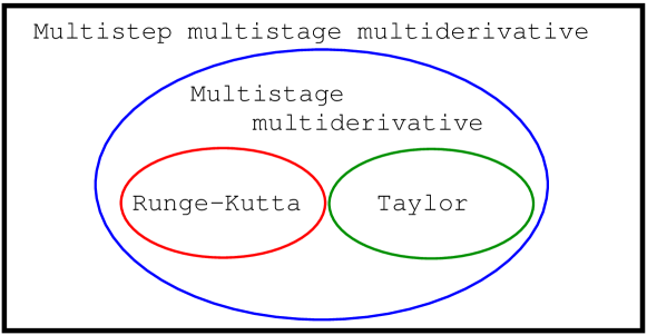
Numerical methods using multiderivative technology have a long history dating back to at least the early 1940’s, and some of the pioneering work for explicit schemes share a common ancestry with implicit schemes. In 1963, Stroud and Stancu StSt63 applied the quadrature method of Turán Tu50 , which generated an implicit, high-order multiderivative ODE solver. Prior to Turán’s work, in 1940, Obreshkoff Obreschkoff40 derived discrete quadrature formulae for integrating functions, and much like Turán did, Obreshkoff used extra derivatives of the function for his quadrature rules. When extra derivatives are included, one can obtain methods with excellent properties for the numerical integration of ODEs, including high-order accuracy involving fewer quadrature points than would otherwise be required. In 1972, Kastlunger and Wanner KaWa72 used the theory of Butcher trees to show that Turán’s quadrature method could be written as an implicit multiderivative Runge-Kutta scheme. The following year, Hairer and Wanner HaWa73 defined “multistep multistage multiderivative methods”, that to date, has stood the test of time as being a broad categorical definition of numerical methods for solving ODEs. A concise taxonomy of this large class of methods is presented in Figure 1. In particular, their definition contains all Runge-Kutta and all linear multistep methods as well as additional combinations, including so-called general linear methods (c.f. John Butcher’s extensive review papers Butcher85 ; Butcher96 ; Butcher06 for a description of general linear methods). The textbooks of Hairer, Nørsett, and Wanner HaWa09 ; HaWa06 contain excellent references.

Figure 1: A simple taxonomy of ODE solvers. Multistep multistage multiderivative methods as defined by Hairer and Wanner HaWa73 are the most inclusive class presented in this diagram. Our focus is on multistage multiderivative methods that include Runge-Kutta (a.k.a. multistage) and Taylor (a.k.a. multiderivative) as special cases.

Our current focus is on explicit versions of multiderivative Runge-Kutta schemes, which needless to say, also have a long history of development. Despite their age, these methods have seen little to no attention outside the ODE community, yet given the direction of modern computer architecture, many of these methods may see use for solving PDEs in the near future. In 1952, Rudolf Zurmühl Zurm52 investigated multiderivative Runge-Kutta integrators, and later on, Erwin Fehlberg Fehlberg60 ; Fehlberg64 derived an explicit multiderivative Runge-Kutta methods. Early versions of Fehlberg’s method applied a single-derivative Runge-Kutta method to the modified variable that is constructed by subtracting out $m$-derivatives of the original variable. A decade later, Kastlunger and Wanner KaWa72-RK extended Butcher’s method to multiderivative Runge-Kutta methods. In their work, they defined the order conditions for the coefficients in a multiderivative Butcher tableau, and in addition, they showed that Fehlberg’s method Fehlberg60 ; Fehlberg64 can be written as a multiderivative Runge-Kutta process with $m$-derivatives taken at a single node. During that same decade, Shintani Shintani71 ; Shintani72 worked on multiderivative Runge-Kutta methods. Also in the 1970’s, Bettis and Horn BettisHorn76 revisited Fehlberg’s scheme and reformulated it as an embedded Taylor method: for their celestial mechanics problem, they describe how the necessary Taylor series coefficients can be generated with little to no additional cost. A decade later and unaware of the full history of the methods, Mutsui Mitsui82 also worked on Runge-Kutta methods that leveraged extra information with extra derivatives.

The most recent work on explicit multiderivative integrators appears to focus on redefining order conditions and demonstrating examples of methods from this class, much of which has been carried out independently from previous work. In 1986, Gekeler and Widmann GeWi86 used the theory of Butcher trees to define the correct order conditions for multiderivative Runge-Kutta methods. In their work, they presented families of methods with orders ranging between four and seven. Goeken and Johnson GoJo99 ; GoJo00 were unaware of the long standing history of explicit multiderivative methods, and they derived their own versions of explicit methods that are sub-optimal. Within the past decade, Yoshida and Ono OnYo03 ; OnYo04 and Chan and Tsai ChTs10 used the theory of Butcher trees to define order conditions and presented numerous examples. The primary difference between the latter two works is the following: Chan and Tsai used multiple stages for their methods, and they restrict their attention to using two derivatives of the unknown function; Yoshida and Ono restrict their attention to two-stage methods, and they admit arbitrarily many derivatives of the unknown function to be evaluated at every quadrature point. In other very recent work, Nguyen-Ba, Božić, Kengne and Vaillancourt BaBo09 derived a nine-stage explicit multiderivative Runge-Kutta scheme that makes use of extra derivatives at a single quadrature point only, much like the schemes Fehlberg originally investigated Fehlberg60 ; Fehlberg64 . In doing so, the order conditions become simpler to navigate.

For the purposes of solving hyperbolic conservation laws, we view using at most two-derivatives of the function as the most appropriate choice given the opportunity to retain portable code. Hyperbolic problems require a definition of the Jacobian of the flux function, which is precisely the term required to define a two-derivative scheme. Investigations into methods using extra derivatives would make for interesting future research.

2.2 Multistage multiderivative methods: some definitions

Consider a system of ODEs, defined by

$$\dot{y}=L(y),\quad y(0)=y_{0},\quad t>0.$$ (6)

We use the letter $L$ in place of $f$ to avoid conflict with the flux function defined later on in equation (19). Without loss of generality, we assume the system is autonomous. Multiderivative methods make use of extra derivatives of (6). If we take a single time derivative of (6), we see that

$$\ddot{y}=\dot{L}=L^{\prime}(y)\,\dot{y}=\frac{\partial L}{\partial y}L(y),$$ (7)

where $\frac{\partial L}{\partial y}$ denotes the partial derivative of $L$ with respect to $y$.

Higher derivatives can be computed recursively. Define the $m^{th}$ derivative of $y$ as $y^{(m)}:=\frac{d^{m}y}{dt^{m}}$, and observe that $y^{(m+1)}=L^{(m)}(y)$. Using the chain rule, we see that

$$y^{(m+1)}=L^{(m)}(y)=\frac{\partial L^{(m-1)}}{\partial y}\dot{y}=\frac{\partial L^{(m-1)}}{\partial y}L(y),\quad m\in\mathbb{Z}_{\geq 1}.$$ (8)

We note that these functions can be computed analytically for ODEs, especially given access to symbolic differentiation software. For PDEs, these higher derivatives will require the use of the Cauchy Kowalewski procedure from equation (5), together with definitions for higher-order spatial derivatives. It will be shown in §§3.2 and 4.2 that WENO and DG make use of very different techniques for defining these higher time derivatives.

Definition 1

Given a collection $\{a^{(m)}_{ij},b^{(m)}_{i}\}$ of real scalars, a multiderivative Runge-Kutta scheme with $s$-stages and $r$-derivatives is any update of the form

$$y_{n+1}=y_{n}+\sum_{m=1}^{r}\Delta t^{m}\sum_{i=1}^{s}b^{(m)}_{i}L^{(m-1)}(y^{(i)}),$$ (9)

where intermediate stage values are given by

$$y^{(i)}=y_{n}+\sum_{m=1}^{r}\Delta t^{m}\sum_{j=1}^{s}a^{(m)}_{ij}L^{(m-1)}(y^{(j)}),$$ (10)

and the total time derivatives of $L$ are given by equation (8). If $a^{(m)}_{ij}=0$ whenever $i\leq j$, the method is explicit, otherwise it is implicit.

We remark that both Taylor and traditional Runge-Kutta methods are special cases Definition 1: setting $r=1$ produces traditional Runge-Kutta methods, and setting $s=1$ produces the Taylor class of methods, with no degrees of freedom for choosing the $b_{i}^{(m)}$. In Table 1, we present the complete Butcher tableau for a multiderivative Runge-Kutta method, and in Table 2, we present the Butcher tableau for the $r^{th}$-order explicit Taylor method.

Table 1: Butcher tableau for a multiderivative Runge-Kutta method. Each $c_{i},a_{ij}^{(m)}$ and $b_{i}^{(m)}$ are real coefficients that define the method using Definition 1. For simplicity, we assume time independence, and so the $c_{i}$ play no factor in the discretization. In addition, we have $c_{i}=c_{i}^{(m)}$, which in general, does not need to be the case. Classical Runge-Kutta methods are special cases of this form, where $r=1$, and $a^{(0)}_{ij}=a_{ij}$ where the $a_{ij}$ are the coefficients for the (single-derivative) Runge-Kutta method. Explicit Taylor methods have no degrees of freedom, nor stages.

$c_{1}$	$a_{11}^{(1)}$	$\cdots$	$a_{1s}^{(1)}$		$a_{11}^{(r)}$	$\cdots$	$a_{1s}^{(r)}$
$\vdots$	$\vdots$	$\ddots$	$\vdots$	$\cdots$		$\ddots$
$c_{s}$	$a_{s1}^{(1)}$	$\cdots$	$a_{ss}^{(1)}$		$a_{s1}^{(r)}$	$\cdots$	$a_{ss}^{(r)}$
	$b_{1}^{(1)}$	$\cdots$	$b_{s}^{(1)}$	$\cdots$	$b_{1}^{(r)}$	$\cdots$	$b_{s}^{(r)}$

Table 2: Butcher tableau for the explicit Taylor method. Here, we present the Butcher coefficients for the $r^{th}$-order explicit Taylor method: $y_{n+1}=y_{n}+\sum_{m=1}^{r}\Delta t^{m}L^{(m-1)}(y_{n})$, where the $L^{(m-1)}$ describe total time derivatives of equation (6) given by equation (8). Note that there are no degrees of freedom for choosing the $b_{i}^{(m)}$, because they are prescribed by $b_{1}^{(m)}=1/m!$.

$0$
	$1$	$1/2!$	$\cdots$	$1/m!$	$\cdots$	$1/r!$

Our definition is an equivalent, yet distinctly different version of what can be found in other sources (c.f. HaWa09 ). It is possible to define intermediate stages through defining and saving $L^{(m)}(y^{(i)})$, but we prefer Definition 1 because of the potential for a low storage implementation, at the cost of recomputing previously observed values. For hyperbolic conservation laws, we consider methods that use at most two-derivatives to be the most portable given that users must have access to the eigen-decomposition of their problem.

Definition 2

Given a collection $\{a^{(1)}_{ij},a^{(2)}_{ij},b^{(1)}_{i}b^{(2)}_{i}\}$ of real scalars, an $s$-stage, two-derivative Runge-Kutta (TDRK) scheme is any update of the form

$$y_{n+1}=y_{n}+\Delta t\sum_{i=1}^{s}b^{(1)}_{i}L(y^{(i)})+\Delta t^{2}\sum_{i=1}^{s}b^{(2)}_{i}\dot{L}(y^{(i)}),$$ (11)

where intermediate stage values are given by

$$y^{(i)}=y_{n}+\Delta t\sum_{j=1}^{s}a^{(1)}_{ij}L(y^{(j)})+\Delta t^{2}\sum_{j=1}^{s}a^{(2)}_{ij}\dot{L}(y^{(j)}).$$ (12)

If $a^{(m)}_{ij}=0$ for all $i\leq j$, the method is explicit.

Before presenting examples of methods from this class, we would like to draw some comparisons between the popular special cases of the multistep multistage multiderivative methods. Our aim is to discuss advantages each method has for being coupled with numerical PDE solvers, and in particular, we would like to focus on which methods have promise for working well with new computer architectures.

Traditional Runge-Kutta methods are far and wide the most popular for solving hyperbolic conservation laws, yet we see room for improvement given the current direction of computer architecture. Runge-Kutta methods are easy to implement, and therefore, they are the most portable of all multistage multiderivative methods. They are self-starting and can easily change their time step size, which is an important characteristic to have for solving hyperbolic conservation laws. In addition, when compared with their natural counterpart, the Adams family of methods (e.g. linear multistep methods), Runge-Kutta methods have stability regions that are more favorable for hyperbolic problems. For example, on a purely oscillatory problem, the maximum stable time step for classical fourth-order Runge-Kutta is given by $|z|\leq\sqrt{8}\approx 2.8$, where $z=\lambda\Delta t$ is purely imaginary. For the same cost and identical storage, one would be able to take four time steps with fourth-order Adams Bashforth. Even after rescaling, the maximum stable time step for the equivalent Adams method would be restricted to $|z|\lessapprox 1.72$. It would seem that Runge-Kutta methods are ideally suited for solving hyperbolic conservation laws. They can be derived to require low-storage Williamson80 ; Ke08 ; Ke10 ; NieDieBu12 , can be designed to acquire strong stability preserving (SSP) properties GoShuTa01 ; Go05 ; Ke08 , and are very portable, especially given that they are self starting. However, traditional Runge-Kutta methods are not optimal with their memory usage, and to date, even the low-storage Runge-Kutta methods require many stages, and therefore they may require considerable communication overhead when compared to pure Taylor schemes.

Taylor methods lie on the other extreme of the multistage multiderivative methods: we claim that they can be implemented to have optimally low-storage for hyperbolic problems, and can contain minimal communication overhead. However, pure Taylor methods are the least portable of the time integrators discussed here. In order to implement a high-order Taylor (e.g. Lax-Wendroff) method for solving a PDE, one needs to have access to high derivatives of the unknown, which puts them out of reach from many scientists. We recognize that this can certainly be done for very complicated problems TaDuBaDiMu07 , but it is difficult to convince users of legacy codes to modify them in order to reach high-order accuracy. On the plus side, high-order Taylor methods contain favorable stability regions for hyperbolic conservation laws, and given that they’re single-step methods, they have nominal communication overhead. However, the only degrees of freedom allowed when choosing these methods is the spatial discretization, given that the time coefficients come directly from the Taylor series.

Given that multiderivative Runge-Kutta methods are a generalization of traditional Runge-Kutta and pure Taylor methods, it is possible to design methods from this class that can retain desirable qualities from each sub-class. In order to retain portability, we view multiderivative Runge-Kutta methods that use at most two-derivatives as optimal for hyperbolic conservation laws, especially given that most codes already have access to, or at least users would be willing to implement the Jacobian of the flux function. Beyond two-derivatives, we would argue the “many”-derivative Runge-Kutta methods start to lose their portability. However, given the large size of this class, there is much room for investigation into what methods work “best” with modern architectures.

2.3 Multistage multiderivative methods: building blocks and examples

Our aim is to describe how to take a multiderivative method from the ODE literature and formulate a hyperbolic solver using that method. In this subsection, we describe a simple building block that can be generalized to accommodate all explicit multistage multiderivative methods.

The building block we will focus on for the remainder of this paper is given by the following:

$$y=y_{n}+\left(\alpha{\Delta t}L(y_{n})+\beta\Delta t^{2}\dot{L}(y_{n})\right)+\left(\alpha^{*}{\Delta t}L(y^{*})+\beta^{*}\Delta t^{2}\dot{L}(y^{*})\right).$$ (13)

In this equation, $y$ could be the full update, as in $y=y_{n+1}$ from equation (11) or a stage value $y=y^{(i)}$ from equation (12). The key to using this equation to solve PDEs is to provide a definition for $L$ and $\dot{L}$.

We prefer introducing $\alpha$ and $\beta$ over $a_{ij}^{(m)}$ and $b_{i}^{(m)}$ from Definitions 1 and 2 because these letters delete unnecessary indices and the upcoming descriptions for the PDE methods will introduce further indices that would become cumbersome.

Remark 1

Extensions to multistage, ‘many’-derivative methods follow by adding extra terms to equation (13).

More stages require more terms to be added to (13). For example, a three stage, two-derivative method is entirely defined after defining updates of the form:

$$y=y_{n} +\left(\alpha\Delta tL(y_{n})+\beta\Delta t^{2}\dot{L}(y_{n})\right)+\left(\alpha^{*}\Delta tL(y^{*})+\beta^{*}\Delta t^{2}\dot{L}(y^{*})\right)$$ (14)

$$+\left(\alpha^{**}\Delta tL(y^{**})+\beta^{**}\Delta t^{2}\dot{L}(y^{**})\right)$$

for arbitrary values of $\alpha$ and $\beta$. Again, the $y$ in this equation can be a single stage value $y=y^{(i)}$ as in equation (12), or a full update, as in equation (11).

We point out that three-derivative, two-stage methods can be formulated with

$$y=y_{n} +\left(\alpha\Delta tL(y_{n})+\beta\Delta t^{2}\dot{L}(y_{n})+\gamma\Delta t^{3}\ddot{L}(y_{n})\right)$$ (15)

$$+\left(\alpha^{*}\Delta tL(y^{*})+\beta^{*}\Delta t^{2}\dot{L}(y^{*})+\gamma^{*}\Delta t^{3}\ddot{L}(y^{*})\right).$$

Note that setting $\alpha=1$, $\beta=1/2$ and $\alpha^{*}=\beta^{*}=0$ in equation (13) produces the second-order Taylor method, and setting $\alpha=1$, $\beta=1/2$, $\gamma=1/6$ and $\alpha^{*}=\beta^{*}=\gamma^{*}=0$ in equation (15) produces the third order Taylor method.

2.3.1 Multistage multiderivative methods: some examples

We now describe how equation (13) can be used to construct multiderivative methods. We assert that these methods have not necessarily been optimized for hyperbolic problems; our chief objective is to demonstrate how to implement these methods. An investigation into optimized schemes will be pursued in the future.

A third order, two-stage, two-derivative method (TDRK3) ChTs10 is given by:

$$y^{*} =y_{n}+\Delta tL(y_{n})+\frac{(\Delta t)^{2}}{2}\dot{L}(y_{n}),$$ (16)

$$y_{n+1} =y_{n}+\Delta t\left(\frac{2}{3}L(y_{n})+\frac{1}{3}L(y^{*})\right)+\frac{\Delta t^{2}}{6}\dot{L}(y_{n}).$$

This method can be constructed by first inserting

$$\alpha=1,\quad\beta=1/2,\quad\alpha^{*}=\beta^{*}=0,$$

into equation (13) to construct the intermediate stage, and the final update is given by selecting

$$\alpha=1,\quad\beta=1/6,\quad\alpha^{*}=0\quad\text{and}\quad\beta^{*}=1/3.$$

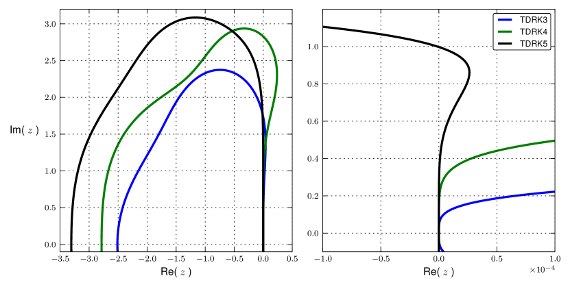
The Butcher tableau for this method is provided in Table 3, and the region of absolute stability is plotted in Figure 2, which is identical to any three stage classical Runge-Kutta method.

Table 3: Butcher tableau for a third-order two-derivative method. Presented here are the coefficients as in Table 1 for an explicit, third-order method ChTs10 . Note that all diagonal and upper-triangular entries are zero, meaning that the scheme is explicit.

$0$	0	0	0	0
$1$	$1/2$	0	$1/8$	$0$
	$2/3$	$1/3$	$1/6$	$0$

Figure 2: Regions of absolute stability. Here, we plot the regions of absolute stability for three different two-derivative methods that are derived in Chan and Tsai ChTs10 : TDRK3 (16), TDRK4 (18) and TDRK5 (17) which are in order of smallest to largest. The picture on the right is a zoomed in picture of the imaginary axis. Note that the third and fourth-order methods have regions of absolute stability identical to classical three and four stage, respectively, RK methods. Of particular importance for hyperbolic problems is the fact that each of these integrators contain part of the imaginary axis bLe02 .

A fifth-order, three-stage, two-derivative method ChTs10 is given by:

$$y^{*} =y_{n}+\frac{2}{5}\Delta tL(y_{n})+\frac{2}{25}\Delta t^{2}\dot{L}(y_{n}),$$ (17)

$$y^{**} =y_{n}+\Delta tL(y_{n})+\Delta t^{2}\left(-\frac{1}{4}\dot{L}(y_{n})+\frac{3}{4}\dot{L}(y^{*})\right),$$

$$y_{n+1} =y_{n}+\Delta tL(y_{n})+\Delta t^{2}\left(\frac{1}{8}\dot{L}(y_{n})+\frac{25}{72}\dot{L}(y^{*})+\frac{1}{36}\dot{L}(y^{**})\right).$$

This method can be constructed by first inserting

$$\alpha=2/5,\quad\beta=2/25,\quad\alpha^{*}=\beta^{*}=0,\quad\alpha^{**}=\beta^{**}=0$$

into equation (14) to produce $y^{*}$, followed by inserting

$$\alpha=1,\quad\beta=-1/4,\quad\alpha^{*}=0,\quad\beta^{*}=3/4,\quad\alpha^{**}=\beta^{**}=0,$$

into (14) to produces a third stage, $y^{**}$. The final update is then given by selecting

$$\alpha=1,\quad\beta=1/8,\quad\alpha^{*}=\alpha^{**}=0,\quad\beta^{*}=\frac{25}{72}\quad\text{and}\quad\beta^{**}=\frac{1}{36}.$$

The Butcher tableau for this method is provided in Table 4, and the region of absolute stability is plotted in Figure 2.

Table 4: Butcher tableau for a fifth-order, three-stage, two-derivative method. Presented here are the coefficients as in Table 1 for an explicit, fifth-order method ChTs10 . Note that all diagonal and upper-triangular entries are zero, meaning that the scheme is explicit. We remark that this scheme has not necessarily been optimized given that some entries were zeroed out by choice in order to reduce the complexity of the order conditions. However, we present this example given that it contains a favorable stability region because it contains part of the imaginary axis (c.f. Figure 2).

$0$	0	0	0	0	0	0
$2/5$	$2/5$	0	0	$2/25$	0	0
$1$	$1$	0	0	$-1/4$	$3/4$	0
	$1$	0	0	$1/8$	$25/72$	$1/36$

2.3.2 Multistage multiderivative methods: the canonical example

The example used for the remainder of this work will now be presented. There is a unique combination for an $s=2$-stage method that produces fourth-order accuracy KaWa72-RK ; OnYo04 ; ChTs10 . This method, which we refer to as TDRK4, can be written as

$$y^{*} =y_{n}+\frac{\Delta t}{2}L_{n}+\frac{(\Delta t/2)^{2}}{2}\dot{L}(y_{n}),$$ (18)

$$y_{n+1} =y_{n}+\Delta tL_{n}+\frac{\Delta t^{2}}{2}\left[\frac{1}{3}\left(\dot{L}(y_{n})+2\dot{L}(y^{*})\right)\right],$$

The Butcher tableau for this method is presented in Table 5, and the region of absolute stability is plotted in Figure 2. Note that the region of absolute stability is identical to any four-stage, fourth-order Runge-Kutta method.

We choose to use this method as our canonical example for three reasons. First, this example is the simplest scheme that does not fall under the Taylor or Runge-Kutta umbrella, and therefore serves as a demonstrative example of new methods that can be found from this class. Second, this method has been optimized for low storage and high-order accuracy given two stages, and two-derivatives, and thirdly, this method works well for hyperbolic problems.

Table 5: Butcher tableau for the multiderivative method investigated in this work. Presented here are the coefficients as in Table 1 for the explicit, fourth-order method, TDRK4 presented in equation (18). Note that all diagonal and upper-triangular entries are zero, meaning that the scheme is explicit.

$0$	0	0	0	0
$1/2$	$1/2$	0	$1/8$	$0$
	$1$	$0$	$1/6$	$1/3$

Given that our goal is to describe how to implement the large class of explicit multistage multiderivative methods for solving PDEs, for simplicity of exposition, we use this method as our canonical example of a method from this class. In addition, we claim that a complete description for this scheme will provide the necessary mechanisms for extension and investigation into integrators containing extra stages. These integrators can be constructed to be even higher order accurate and contain favorable stability regions. For example, all of the methods presented in Chan and Tsai ChTs10 can be implemented using our description with a straight-forward extension of what follows.

Observe that the TDRK4 method in equation (18) can be constructed from of equation (13), with the first stage given by

$$\alpha=1/2,\quad\beta=1/8,\quad\alpha^{*}=\beta^{*}=0,$$

and the update given by

$$\alpha=1,\quad\beta=1/6,\quad\alpha^{*}=0\quad\text{and}\quad\beta^{*}=1/3.$$

This completes our description of the multiderivative Runge-Kutta scheme, and it bears repeating that without loss of generality, we will use method (18) as our canonical example of a method from this class. Given that the focus of this work is how to implement this scheme for solving hyperbolic PDEs, we still need to describe how to discretize in space.

3 The finite difference WENO method

The finite difference weighted essentially non-oscillatory (WENO) method has many variations and a long history of development. The original method was developed by Shu and Osher ShuOsher87 ; ShuOsher89 , and later analyzed and further developed by Shu and his collaborators JiangShu96 ; Shu97 ; Shu01 . For a recent comprehensive review of the many variations of WENO schemes, see Chi-Wang Shu’s extensive review paper Shu09 . In this work, we consider the fifth-order WENO-Z scheme HeAsPo05 ; BoCaCoWai08 ; CaCoDo11 , that is an improvement of the classical fifth-order Jiang and Shu (WENO-JS) scheme JiangShu96 . The underlying choice of the reconstruction procedure is not central to this work and our description will be generic enough to accommodate most variations of the classical WENO method. However, given that there are many options, we explain the minimal details necessary to reproduce the present work.

In §3.1 we present the classical MOL formulation for the WENO method. In §3.2 we describe the extension of multiderivative ODE integrators presented in §§2.2–2.3, to formulate the multiderivative WENO method that is the subject of this section. In §4.2 we will see that the extension of multiderivative ODE methods from §2 to the DG method requires a very different approach.

3.1 The finite difference WENO method: MOL formulation

We begin our description with a reduction of (1) to a 1D conservation law:

$$q_{,t}+f(q)_{x}=0,\quad q(0,x)=q_{0}(x),\quad x\in\Omega=[a,b].$$ (19)

Here, we follow the standard convention of naming our flux function $f$ in place of $R$. Moreover, (19) is hyperbolic if the Jacobian $f^{\prime}(q)=R\Lambda R^{-1}$ is diagonalizable with real eigenvalues for all $q$ in the domain of interest.

The spatial discretization for a finite difference method seeks a point-wise approximation to the exact solution of (19) at a finite collection of points. We start with a uniform discretization of $[a,b]$ using $m_{x}$ points:

$$\Delta x=(b-a)/m_{x},\quad\quad x_{i}=a+(i-1/2)\Delta x,\quad\quad i\in\left\{1,2,\ldots,m_{x}\right\},$$ (20)

and we seek values $q_{i}$ that approximate the exact solution at each grid point, $q_{i}(t)\approx q(t,x_{i})$.

In order to write (19) in discrete flux-difference form so we can have a conservative method, we begin by defining an implicit sliding function $h$ through

$$f\left(q(t,x)\right)=\frac{1}{\Delta x}\int_{x-\Delta x/2}^{x+\Delta x/2}h(t,x)\,dx.$$ (21)

With this definition in place, we have the nice result that

$$\frac{\partial f}{\partial x}\left(q(t,x_{i})\right)=\frac{1}{\Delta x}\left[h\left(t,x_{i+1/2}\right)-h\left(t,x_{i-1/2}\right)\right],$$ (22)

which is precisely what is needed to define a discrete flux difference formulation of $q_{t}=-f_{x}$. The MOL formulation for the finite difference scheme defines interpolated values $h_{i+1/2}$ that approximate $h\left(t,x_{i+1/2}\right)$ to high-order accuracy,

$$\frac{1}{\Delta x}\left(h_{i+1/2}-h_{i-1/2}\right)=\frac{\partial f}{\partial x}\left(q(t,x_{i})\right)+\mathcal{O}\left(\Delta x^{M}\right).$$ (23)

Moreover, an astute observation means that $h$ need never be computed Shu97 ; Shu09 : define cell averages of $h(t,x)$ as

$$\bar{h}_{i}:=\frac{1}{\Delta x}\int_{x_{i-1/2}}^{x_{i+1/2}}h(t,x)\,dx,$$ (24)

then observe that $f(q_{i}(t))=\bar{h}_{i}$, and therefore point values of $f$ can be interpreted as cell averages of $h$. After defining an appropriate interpolating algorithm for producing high-order interface values $h_{i+1/2}$ from cell averages $\bar{h}_{i}$, the full MOL formulation is given by,

$$\frac{d}{dt}q_{i}(t)=-\frac{1}{\Delta x}\left(h_{i+1/2}-h_{i-1/2}\right).$$ (25)

This scheme is automatically conservative as it is written in flux difference form. Usually one applies a high-order explicit Runge-Kutta integrator to (25), which results in what is normally called the Runge-Kutta WENO (RK-WENO) method.

3.1.1 The finite difference WENO method: the reconstruction procedure

A conservative reconstruction procedure requires a single value $h_{i+1/2}$ for equation (25) to be defined at each grid interface. In the ensuing discussion, we suppress the time dependence of $h$, and assume that we have known cell averages $\bar{h}_{i}$ for a function $h=h(x)$. The fifth-order WENO method uses a five point stencil shifted to the left or right of the interface:

$$h_{i+1/2}^{+} :=WENO5^{+}[\bar{h}_{i-2},\bar{h}_{i-2},\bar{h}_{i-1},\bar{h}_{i},\bar{h}_{i+2}],$$

$$h_{i+1/2}^{-} :=WENO5^{-}[\bar{h}_{i-1},\bar{h}_{i},\bar{h}_{i+1},\bar{h}_{i+2},\bar{h}_{i+3}].$$

Here, we define coefficients for the function $WENO5^{+}$, and note that by symmetry, the reconstruction procedure weighted in the other direction can be observed by flipping the stencil:

$$WENO5^{-}[\bar{h}_{i-1},\bar{h}_{i},\ldots\bar{h}_{i+3}]:=WENO5^{+}[\bar{h}_{i+3},\bar{h}_{i+2},\ldots\bar{h}_{i-1}].$$ (26)

Three sub-stencils $S_{0}=\{\bar{h}_{i-2},\bar{h}_{i-1},\bar{h}_{i}\}$, $S_{1}=\{\bar{h}_{i-1},\bar{h}_{i},\bar{h}_{i+1}\}$, and $S_{2}=\{\bar{h}_{i},\bar{h}_{i+1},\bar{h}_{i+2}\}$ uniquely define three quadratic polynomials $p_{j}(x)$ that have the same cell averages for each element in their stencil. Each polynomial defines a competing value for $h(x_{i+1/2})$ with $h^{(j)}_{i+1/2}=p_{j}(x_{i+1/2})$:

$$h^{(0)}_{i+1/2} =\phantom{-}\frac{1}{3}\bar{h}_{i-2}-\frac{7}{6}\bar{h}_{i-1}+\frac{11}{6}\bar{h}_{i},$$ (27a)

$$h^{(1)}_{i+1/2} =-\frac{1}{6}\bar{h}_{i-1}+\frac{5}{6}\bar{h}_{i\phantom{-1}}+\frac{1}{3}\bar{h}_{i+1},$$ (27b)

$$h^{(2)}_{i+1/2} =\phantom{-}\frac{1}{3}\bar{h}_{i\phantom{-1}}+\frac{5}{6}\bar{h}_{i+1}-\frac{1}{6}\bar{h}_{i+2}.$$ (27c)

The linear weights $\gamma_{j}=\left\{1/10,\,3/5,\,3/10\right\}$ are defined as the unique linear combination of equations (27a)-(27c) that yields a fifth-order accurate point value for $h(x_{i+1/2})$:

$$h_{i+1/2}=\gamma_{0}h^{(0)}_{i+1/2}+\gamma_{1}h^{(1)}_{i+1/2}+\gamma_{2}h^{(2)}_{i+1/2}.$$ (28)

The WENO procedure replaces the linear weights $\gamma_{j}$ with nonlinear weights $\omega_{j}$ that are necessary in regions with strong shocks. The Jiang and Shu smoothness indicators $\beta_{j}$ place a quantitative measure on the smoothness of each stencil based on a Sobolev norm:

$$\beta_{j}:=\sum_{l=1}^{k}\Delta x^{2l-1}\int_{x_{i-1/2}}^{x_{i+1/2}}\left(\frac{d^{l}}{dx^{l}}p_{j}(x)\right)^{2}\,dx,$$ (29)

which for our fifth order method, are given by

$$\begin{aligned} \beta_{0}&=\frac{13}{12}\left(\bar{h}_{i-2}-2\bar{h}_{i-1}+\bar{h}_{i}\right)^{2}+\frac{1}{4}\left(\bar{h}_{i-2}-4\bar{h}_{i-1}+3\bar{h}_{i}\right)^{2},\\ \beta_{1}&=\frac{13}{12}\left(\bar{h}_{i-1}-2\bar{h}_{i}+\bar{h}_{i+1}\right)^{2}+\frac{1}{4}\left(\bar{h}_{i-1}-\bar{h}_{i+1}\right)^{2},\\ \beta_{2}&=\frac{13}{12}\left(\bar{h}_{i}-2\bar{h}_{i+1}+\bar{h}_{i+2}\right)^{2}+\frac{1}{4}\left(3\bar{h}_{i}-4\bar{h}_{i+1}+\bar{h}_{i+2}\right)^{2}.\end{aligned}$$ (30)

The non-linear WENO-Z weights $\omega^{z}_{j}$ are a slight modification of the classical weights $\omega_{j}$. The new weights require the computation of a single additional parameter $\tau^{5}=\left|\beta_{2}-\beta_{0}\right|$:

$$\omega^{z}_{k}=\frac{\tilde{\omega}^{z}_{k}}{\sum_{l=0}^{2}\tilde{\omega}^{z}_{l}},\quad\tilde{\omega}^{z}_{k}=\frac{\gamma_{k}}{\beta^{z}_{k}},\quad\beta^{z}_{k}=1+\left(\frac{\tau^{5}}{\beta_{k}+\epsilon}\right)^{p}.$$ (31)

We use the power parameter $p=2$ and regularization parameter $\epsilon=10^{-12}$ for all of our simulations. With these definitions in place, the final interpolated value is defined as

$$WENO5^{+}[\bar{h}_{i-2},\ldots\bar{h}_{i+2}]:=\omega^{z}_{0}h^{(0)}_{i+1/2}+\omega^{z}_{1}h^{(1)}_{i+1/2}+\omega^{z}_{2}h^{(2)}_{i+1/2}.$$ (32)

3.1.2 The finite difference WENO method: MOL formulation for systems

For a system of conservation laws, the reconstruction procedure described in §3.1.1 is carried out locally on each of the scalar characteristic variables:

Finite difference WENO procedure for 1D systems

1. For each $i$, evaluate $f_{i}=f(q_{i})$ at each mesh point and compute average values of $q$ at the half grid points

   $$q^{*}_{i-1/2}=\frac{1}{2}\left(q_{i}+q_{i-1}\right).$$ (33)

   Roe averages Roe81 may be used in place of (33), but all the results presented in this work use this arithmetic average.

2. Compute the left and right eigenvalue decomposition of $f^{\prime}(q)=R\Lambda R^{-1}$ at the half-grid points:

   $$R_{i-1/2}=R(q^{*}_{i-1/2}),\quad R^{-1}_{i-1/2}=R^{-1}(q^{*}_{i-1/2}).$$ (34)

   Compute $\alpha:=\max_{i}|f^{\prime}(q^{*}_{i-1/2})|$ as the fastest wave speed in the entire system. For stability, we follow the common practice of increasing $\alpha$ by exactly 10% in order to completely contain the fastest wave speed, that is, we set $\alpha=1.1\cdot\max_{i}|f^{\prime}(q^{*}_{i-1/2})|$. The value $|f^{\prime}(q)|$ is the maximum absolute value of all eigenvalues of the Jacobian, $f^{\prime}(q)$.

3. For each $i$, determine the weighted ENO stencil $\{i+r\}$ surrounding $i$. In fifth order WENO, the full stencil is given by $r\in\{-3,-2,-1,0,1,2\}$. Project each $q_{i+r}$ and flux values $f_{i+r}$ onto the characteristic variables using $R^{-1}_{i-1/2}$:

   $$w_{i+r}=R^{-1}_{i-1/2}\cdot q_{i+r},$$ (35a)

   $$g_{i+r}=R^{-1}_{i-1/2}\cdot f_{i+r}.$$ (35b)

   Apply Lax-Friedrichs flux splitting on $g_{i+r}$:

   $$g^{\pm}_{i+r}=\frac{1}{2}\left(g_{i+r}\pm\alpha\,w_{i+r}\right).$$ (36)

   As an alternative, one could use a local wave speed. Note that for each component, these definitions automatically satisfy $\frac{dg^{+}}{dw}\geq 0$ and $\frac{dg^{-}}{dw}\leq 0$.

4. Perform a WENO reconstruction on the characteristic variables. Use the stencil which uses an extra point on the upwind direction for defining $g^{\pm}$:

   $$\hat{g}^{+}_{i-1/2} =WENO5^{+}\left[g^{+}_{i-3},g^{+}_{i-2},g^{+}_{i-1},g^{+}_{i},g^{+}_{i+1}\right],$$

   $$\hat{g}^{-}_{i-1/2} =WENO5^{-}\left[g^{-}_{i-2},g^{-}_{i-1},g^{-}_{i},g^{-}_{i+1},g^{-}_{i+2}\right].$$

   Define $\hat{g}_{i-1/2}:=\hat{g}^{+}_{i-1/2}+\hat{g}^{-}_{i-1/2}$.

5. Using same projection matrix, $R_{i-1/2}$, project characteristic variables back onto the conserved variables:

   $$\hat{f}_{i-1/2}:=R_{i-1/2}\cdot\hat{g}_{i-1/2}.$$ (37)

3.2 The finite difference WENO method: a multiderivative formulation

In order to implement multiderivative methods into the WENO framework, we closely follow previous work on Lax-Wendroff WENO methods QiuShu03 , but in place of relying on a single-step Taylor series, we build intermediate stages of the form given by (13). Consider two ‘stages’, $q^{n}$ and $q^{*}$ that provide a pointwise approximation to the exact solution. If we apply (5) to each $q^{n}$ and $q^{*}$ and insert the result into (13), we see that the starting point for putting together a multiderivative WENO integrator is to define the following for arbitrary values of $\alpha$, $\alpha^{*}$, $\beta$ and $\beta^{*}$:

$$\begin{split}q=q^{n}&-\alpha\Delta tf\left(q^{n}\right)_{\!,\,x}-\alpha^{*}\Delta tf\left(q^{*}\right)_{\!,\,x}\\ &-\beta\Delta t^{2}\left(f^{\prime}(q^{n})q^{n}_{,t}\right)_{\!,\,x}-\beta^{*}\Delta t^{2}\left(f^{\prime}(q^{*})q^{*}_{,t}\right)_{\!,\,x}.\end{split}$$ (38)

Note that we have retained the value $q_{,t}$ in place of substituting $q_{,t}=-f_{,x}$ into the last two terms. This is different than what will be done in §4.2 for the multiderivative DG method. The complete multiderivative WENO method is given by the following:

Multistage multiderivative WENO procedure

1. Given two pointwise approximations $q^{n}$ and $q^{*}$, perform a single WENO reconstruction on each piece to construct the following values:

   $$q^{n}_{i,t}:=-\frac{1}{\Delta x}\left(\hat{f}^{n}_{i+1/2}-\hat{f}^{n}_{i-1/2}\right),\quad q^{*}_{i,t}:=-\frac{1}{\Delta x}\left(\hat{f}^{*}_{i+1/2}-\hat{f}^{*}_{i-1/2}\right).$$ (39)

2. Define the pointwise values ${G}^{n}_{i}:=f^{\prime}\left(q^{n}_{i}\right)q^{n}_{i,t}$ and ${G}^{*}_{i}:=f^{\prime}\left(q^{*}_{i}\right)q^{*}_{i,t}$. Note that we do not need to decompose $q$ onto the characteristic variables.

3. For each $G^{n}$ and $G^{*}$ in Step 2, compute a finite difference approximation to $G^{n}_{,x}$ and $G^{*}_{,x}$. Given that this term inherits an extra factor of $\Delta t$, we can use the fourth-order centered finite difference:

   $$D_{x}G_{i}:=\frac{1}{12\Delta x}\left(G_{i-2}-8G_{i-1}+8G_{i+1}-G_{i+2}\right).$$ (40)

   Using a centered stencil means that the method will automatically be conservative. The complete WENO discretization of (38) is now,

   $$q_{i}=q_{i}^{n}+\alpha\Delta tq^{n}_{i,t}+\alpha^{*}\Delta tq^{*}_{i,t}-\beta\Delta t^{2}D_{x}G^{n}_{i}-\beta^{*}\Delta t^{2}D_{x}G^{*}_{i}.$$ (41)

   This equation defines the building block for creating any two-derivative Runge-Kutta method, because the definitions for $L$ and $\dot{L}$ from Definition 2 are now in place.

We now summarize the entire multiderivative WENO procedure. Given a multiderivative Runge-Kutta scheme, we use a WENO reconstruction procedure to define $q_{,t}$. Higher derivatives $q_{,tt}$, etc. are defined by first using the Cauchy-Kowalewski procedure in (5) to define exact formulas for these terms. The spatial derivatives that show up in these terms are then discretized by using finite differences. Once $q_{,t},q_{,tt}$, etc., have been defined, one uses the coefficients from the multiderivative scheme to construct stages as well as a final update. This entire procedure generalizes both the Lax-Wendroff and RK-WENO methods. For completeness, we prove that the proposed scheme is conservative by showing that equation (41) is conservative for any choice of $\alpha$, $\alpha^{*}$, $\beta$ and $\beta^{*}$ that are defined by the selected multiderivative scheme.

Theorem 1

The proposed multistage multiderivative WENO scheme is mass conservative.

Proof

The final update, $q^{n+1}_{i}$ is given by equation (41) for a collection of coefficients $\alpha$, $\alpha^{*}$, $\beta$ and $\beta^{*}$ that depend on the selected scheme. Summing over $i$ produces

$$\sum_{i}q^{n+1}_{i} =\sum_{i}\left(q^{n}_{i}+\alpha\Delta tq^{n}_{i,t}+\alpha^{*}\Delta tq^{*}_{i,t}-\beta\Delta t^{2}D_{x}G^{n}_{i}-\beta^{*}\Delta t^{2}D_{x}G^{*}_{i}\right)$$ (42a)

$$=\sum_{i}q^{n}_{i}+\alpha\Delta t\sum_{i}q^{n}_{i,t}+\alpha^{*}\Delta t\sum_{i}q^{*}_{i,t}+\beta\Delta t^{2}\sum_{i}D_{x}G_{i}+\beta^{*}\Delta t^{2}\sum_{i}D_{x}G^{*}_{i}.$$ (42b)

Conservation will follow after showing that the last four terms in equation (42b) are zero. First, observe that

$$\sum_{i}q^{n}_{i,t} =-\frac{1}{\Delta x}\sum_{i}\left(\hat{f}^{n}_{i+1/2}-\hat{f}^{n}_{i-1/2}\right)=-\frac{1}{\Delta x}\left(\sum_{i}\hat{f}^{n}_{i+1/2}-\sum_{i}\hat{f}^{n}_{i-1/2}\right)$$ (43a)

$$=-\frac{1}{\Delta x}\left(\sum_{i}\hat{f}^{n}_{i+1/2}-\sum_{i}\hat{f}^{n}_{i+1/2}\right)=0.$$ (43b)

Similarly, $\sum_{i}q^{*}_{i,t}=0$. The last two terms sum to zero because a central difference stencil is used:

$$\sum_{i}D_{x}G^{n}_{i} =\frac{1}{12\Delta x}\sum_{i}\left(G^{n}_{i-2}-8G^{n}_{i-1}+8G^{n}_{i+1}-G^{n}_{i+2}\right)$$ (44a)

$$=\frac{1}{12\Delta x}\left(\sum_{i}G^{n}_{i-2}-8\sum_{i}G^{n}_{i-1}+8\sum_{i}G^{n}_{i+1}-\sum_{i}G^{n}_{i+2}\right)$$ (44b)

$$=\frac{1}{12\Delta x}\left(\sum_{i}G^{n}_{i}-8\sum_{i}G^{n}_{i}+8\sum_{i}G^{n}_{i}-\sum_{i}G^{n}_{i}\right)=0.$$ (44c)

Similarly, $\sum_{i}D_{x}G^{*}_{i}=0$, and therefore $\sum_{i}q^{n+1}_{i}=\sum_{i}q^{n}_{i}$ for all $n$. ∎

Remark 2

Various multistage multiderivative WENO methods can be built by repeated application of (41) with different values of $\alpha,\alpha^{*},\beta$ and $\beta^{*}$.

The procedure for constructing multiderivative WENO methods using (41) is identical to that already presented in §2.3 for ODEs. For example, setting $\beta=\beta^{*}=0$ reproduces Runge-Kutta methods, and setting $\alpha^{*}=\beta^{*}=0$ reproduces the second-order Lax-Wendroff WENO method, provided we define $\alpha=1$, and $\beta=1/2$. The $s=3$-stage analogue of equation (15) for PDEs is given by

$$\begin{split}q_{i}=q_{i}^{n}&+\alpha\Delta tq^{n}_{i,t}+\alpha^{*}\Delta tq^{*}_{i,t}+\alpha^{**}\Delta tq^{**}_{i,t}\\ &-\beta\Delta t^{2}D_{x}G^{n}_{i}-\beta^{*}\Delta t^{2}D_{x}G^{*}_{i}-\beta^{**}\Delta t^{2}D_{x}G^{**}_{i}.\end{split}$$ (45)

In addition, further derivatives can be included, but one would need to revisit (5) before inserting these terms. We would expect that higher derivatives can be approximated using smaller centered finite difference stencils because they get multiplied by increasing powers of $\Delta t$ (c.f. QiuShu03 for further details).

We repeat that equation (41) finishes the spatial discretization of (13). If we appeal to this equation twice we can construct the unique two-stage, fourth-order method, TDRK4 that is the PDE analogue of (18):

$$q^{*}_{i} =q^{n}_{i}-\frac{\Delta t}{2\Delta x}\left(\hat{f}^{n}_{i+1/2}-\hat{f}^{n}_{i-1/2}\right)-\frac{(\Delta t/2)^{2}}{2}\left(D_{x}G_{i}\right);$$ (46a)

$$q^{n+1}_{i} =q^{n}_{i}-\frac{\Delta t}{\Delta x}\left(\hat{f}^{n}_{i+1/2}-\hat{f}^{n}_{i-1/2}\right)-\frac{\Delta t^{2}}{6}\left(D_{x}G_{i}+2D_{x}G^{*}_{i}\right).$$ (46b)

Numerous examples of this WENO scheme are provided in §5, where we compare this method with classical fourth-order Runge-Kutta (RK4), as well as the third-order strong stability preserving (SSP) method of Shu and Osher ShuOsher87 . Before presenting results, we first describe an implementation of a multistage multiderivative discontinuous Galerkin method that will require a different approach to define the higher temporal derivatives.

4 The discontinuous Galerkin (DG) method

The discontinuous-Galerkin (DG) method dates back to 1973 when Reed & Hill ReedHill73 developed the scheme for solving a neutron transport equation. The theoretical framework for the DG method was solidified by Bernardo Cockburn and Chi-Wang Shu through a lengthy series of papers. We refer the reader to their extensive review article and references therein CoShu01 . In this section, we define the notation used for the remainder of this paper and provide minimal details necessary for reproducing this body of work. This section focuses on describing the Runge-Kutta discontinuous Galerkin (RKDG) scheme, and in §4.2, we introduce the multiderivative technology to the DG framework. We use similar notation to that was previously introduced RoSe10 , and for further details on the DG method, we direct the reader the references (e.g. CoShu01 ; Seal12 ).

Similar to the layout of §3, we begin this section with the classical MOL formulation in §4.1, and continue in §4.2 with the proposed multiderivative DG method. We repeat that much like the material from §3.2, the multiderivative DG formulation relies on the multiderivative ODE methods from §2 but requires a very different application of the Cauchy Kowalewski procedure from equation (5).

4.1 The discontinuous Galerkin (DG) method: a MOL formulation

The DG method solves a discretization of the weak formulation of the hyperbolic conservation law (19). The continuous weak formulation can be realized by multiplying (19) with a test function $\varphi$, and integrating by parts over a control volume $\mathcal{T}=[x_{\ell},x_{r}]$:

$$\int_{x_{\ell}}^{x_{r}}\,\varphi q_{,t}\,dx=\int_{x_{\ell}}^{x_{r}}\varphi_{,x}\,f(q)\,dx-\Bigl{(}\left.\varphi f(q)\,\right\rvert_{x_{r}}-\left.\varphi f(q)\,\right\rvert_{x_{\ell}}\Bigr{)}.$$ (47)

We begin our discretization by defining a grid containing $m_{x}$ cells for the domain $[a,b]$, each of whose width is $\Delta x=(b-a)/m_{x}$. The $i^{th}$ grid cell is denoted by $\mathcal{T}_{i}=[x_{i-1/2},x_{i+1/2}]$, where the cell edges are given by $x_{i-1/2}=a+(i-1)\Delta x$, for $i=1,2,\ldots,m_{x}+1$, and the cell centers are given by $x_{i}=a+(i-1/2)\Delta x$, for $i=1,2,\ldots,m_{x}$. For simplicity of exposition, we will restrict our attention to a uniform grid. On this grid we define the broken finite element space

$$W^{h}=\left\{w^{h}\in L^{\infty}(\Omega):\,w^{h}|_{\mathcal{T}}\in P^{p},\,\forall\mathcal{T}\in\mathcal{T}_{h}\right\},$$ (48)

where $h=\Delta x$. The above expression means that on each element $\mathcal{T}$, $w^{h}$ will be a polynomial of degree at most $p$, and no continuity is assumed across element edges. Each element $\mathcal{T}_{i}$ can be mapped to the canonical element $\xi\in[-1,1]$ via the linear transformation

$$x=x_{i}+\xi\,\frac{\Delta x}{2}.$$ (49)

Note that after a change of variables, spatial derivatives obey the following rule: $\frac{\partial}{\partial x}=\frac{2}{\Delta x}\frac{\partial}{\partial\xi}$. For the canonical element, we construct a set of basis functions that are orthonormal with respect to the following inner product:

$$\Bigl{\langle}\varphi^{(\ell)},\,\varphi^{(k)}\Bigr{\rangle}:=\frac{1}{2}\int_{-1}^{1}\varphi^{(\ell)}(\xi)\varphi^{(k)}_{\text{}}(\xi)\ d\xi=\delta_{\ell k},$$ (50)

where $\delta_{\ell k}$ is the Kronecker delta function. This defines the Legendre basis functions:

$$\varphi^{(\ell)}=\Biggl{\{}1,\,\,\,\sqrt{3}\,\xi,\,\,\,\frac{\sqrt{5}}{2}\left(3\xi^{2}-1\right),\,\,\,\frac{\sqrt{7}}{2}(5\xi^{3}-3\xi),\,\,\,\dots\Biggr{\}}.$$ (51)

We consider approximate solutions of the hyperbolic conservation law (19) that are defined by a finite set of coefficients $\left\{Q^{(k)}_{i}\right\}$ of the basis functions $\left\{\varphi^{(k)}\right\}$. When restricted to a single cell $\mathcal{T}_{i}$, the approximate solution $q^{h}$ is

$${q}^{h}(t,x)\Bigl{|}_{\mathcal{T}_{i}}:=q_{i}^{h}(t,\xi)=\sum_{k=1}^{M}Q^{(k)}_{i}(t)\,\varphi_{\text{}}^{(k)}(\xi),$$ (52)

where $M$ is the order of accuracy. The initial conditions are determined from the $L^{2}$-projection of $q^{h}(0,x)$ onto the basis functions,

$$Q^{(k)}_{i}(0):=\Bigl{\langle}{q}_{i}^{h}(0,\xi),\,\varphi_{\text{}}^{(k)}(\xi)\Bigr{\rangle},$$ (53)

which we evaluate using $M$ standard Gaussian quadrature points.

The semi-discrete weak formulation of (19) is given by discretizing (47) with a finite set of basis functions and a finite set of control volumes. Inserting our discrete spatial representation (52) into the continuous weak formulation (47) and using $\varphi=\varphi^{(k)}$ for our test function, we produce the semi-discrete weak formulation

$$\begin{split}\Bigl{\langle}{q}_{i,t}^{h}(t,\xi),\varphi^{(k)}(\xi)\Bigr{\rangle}=&\ \frac{2}{\Delta x}\Bigl{\langle}f\left({q}_{i}^{h}(t,\xi)\right),{{\varphi_{\xi}^{(k)}}}{}(\xi)\Bigr{\rangle}\\ &-\frac{1}{\Delta x}\varphi^{(k)}(\xi=+1)f^{\downarrow}(q^{h}(t,x_{i+1/2})\\ &+\frac{1}{\Delta x}\varphi^{(k)}(\xi=-1)f^{\downarrow}(q^{h}(t,x_{i-1/2})),\end{split}$$ (54)

where the flux values $f^{\downarrow}(q^{h}(t,x_{i-1/2}))$ will be defined through an appropriate Riemann solver. These terms will become responsible for all inter-cell communication.

Before going into the details of the Riemann solver, we seek a simpler representation of (54). We start by defining the first term on the right hand side of (54) as the interior integral

$$N^{(k)}_{i}:=\frac{1}{\Delta x}\int_{-1}^{1}\varphi^{(k)}_{\xi}\left(\xi\right)f\left(q^{h}_{i}(t,\xi)\right)\,d\xi,$$ (55)

and after rescaling, we define the last two terms as

$${F}^{(k)}_{p,i+1/2}:= \ \varphi^{(k)}(\xi=+1)f^{\downarrow}(q^{h}(t,x_{i+1/2})),$$ (56a)

$${F}^{(k)}_{m,i-1/2}:= \ \varphi^{(k)}(\xi=-1)f^{\downarrow}(q^{h}(t,x_{i-1/2})).$$ (56b)

With these definitions in place, the discrete weak formulation can now be compactly written as a large MOL system:

$$\frac{d}{dt}{Q}^{(k)}_{i}(t)=\underbrace{\phantom{\frac{1}{1}}{N^{(k)}_{i}(t)}}_{\text{Interior}}-\underbrace{\frac{1}{\Delta x}\left[{F}^{(k)}_{p,i+1/2}(t)-{F}^{(k)}_{m,i-1/2}(t)\right]}_{\text{Edge}}.$$ (57)

The only remaining piece to describe is how we compute the inter-cell flux values, $f^{\downarrow}(q^{h}(t,x_{i-1/2}))$.

4.1.1 The discontinuous Galerkin (DG) method: a choice of Riemann solvers

Given that the representation of the solution, $q^{h}$, is not forced to be continuous at the cell interfaces, care must be taken when defining the flux values $f^{\downarrow}\left(q^{h}(t,x_{i-1/2})\right)$. One could work with the so-called generalized Riemann solvers which take into account spatially varying function to the left and right of the discontinuity. One could also work with exact solutions for a classical Riemann problem in which one assumes constant states to the left and right of a discontinuity. In this work, we use Rusanov’s method Rusanov61 , which is an approximate Riemann solver that is commonly called the local Lax-Friedrichs (LLF) Riemann solver given its similarity to the Lax-Friedrichs method. Much like the Lax-Friedrichs method, this solver approximates each Riemann problem with two waves with equal speeds traveling in opposite directions, but LLF uses a local speed in place of a global speed to do so.

Evaluating the basis functions to the left and right of a single interface located at $x_{i-1/2}$ provides artificially constant states, defined by a finite sum,

$$Q_{r} =Q^{(1)}_{i}-\sqrt{3}\,Q^{(2)}_{{i}}+\sqrt{5}\,Q^{(3)}_{{i}}-\sqrt{7}\,Q^{(4)}_{{i}}+\cdots$$ (58a)

$$Q_{\ell} =Q^{(1)}_{{i-1}}+\sqrt{3}\,Q^{(2)}_{{i-1}}+\sqrt{5}\,Q^{(3)}_{{i-1}}+\sqrt{7}\,Q^{(4)}_{{i-1}}+\cdots.$$ (58b)

The LLF solver defines a single value based on these two constant states:

$$f^{\downarrow}\left(Q_{l},Q_{r}\right):=\frac{1}{2}\Bigl{[}\left(f\left(Q_{l}\right)+f\left(Q_{r}\right)\right)-\alpha\left(Q_{r}-Q_{l}\right)\Bigr{]}.$$ (59)

We use a local value of $\alpha$, defined by $\alpha=\max\left\{\left|s^{1}\right|,\left|s^{2}\right|\right\}$, where $s^{1}$ and $s^{2}$ are the HLL(E) speeds HaLaLe83 defined by

$$s^{1} =\min\left\{\min_{p}\lambda^{(p)}\left(\hat{Q}\right),\,\min_{p}\lambda^{(p)}\left(Q_{l}\right)\right\},$$ (60a)

$$s^{2} =\max\left\{\max_{p}\lambda^{(p)}\left(\hat{Q}\right),\,\max_{p}\lambda^{(p)}\left(Q_{r}\right)\right\},$$ (60b)

and $\lambda^{(p)}$ are the eigenvalues of $f^{\prime}$. For this work, we take the simple arithmetic average $\hat{Q}=\frac{1}{2}\left(Q_{l}+Q_{r}\right)$, but we point out that Roe averages could also be used Roe81 .

This completes the DG method of lines (MOL) discretization for our PDE. The only remaining part is to evolve the discrete coefficients through time. This is usually performed by explicit, high-order Runge-Kutta methods, resulting in a Runge-Kutta discontinuous Galerkin (RKDG) method. In principle, one may potentially work with this discretization to form a multiderivative integrator, which would require taking a second derivative of (57). However, difficulty will ensue when trying to compute the Jacobian of the complex system of ODEs in (54). Instead, we turn towards the Lax-Wendroff/Cauchy-Kowalewski discontinuous Galerkin methods to define a discrete second derivative.

4.2 The discontinuous Galerkin (DG) method: a multiderivative formulation

In this section, we extend the work of Qiu, Dumbser and Shu QiuDumbserShu05 to accommodate multiderivative technology. An investigation into other fluxes would be an interesting topic of future study, including a comparison of various approximate Riemann solvers using multiderivative technology Qiu07 ; moreover, an investigation into generalized Riemann solvers DuMu06 ; DuBaDiToMuDi08 ; MoCaDuTo12 may yield some interesting results. At present, our current goal is to lay the foundation that would be necessary for such investigations.

Starting with the aim of defining a single stage value (or full update) for a multiderivative integrator, a DG implementation of equation (13) from §2.3 requires the definition of $q_{,tt}$ as well as the definition of $q^{\star}_{,tt}$. Here, we use $q_{,tt}=\left(f^{\prime}(q)f_{x}\right)_{x}$ in place of $q_{,tt}=-\left(f^{\prime}(q)q_{t}\right)_{x}$ which was used in §3.2 for the second derivative. After factoring out a single spatial derivative, we can write (13) as

$$q=q^{n}-\Delta t\Bigl{[}\alpha f^{n}+\alpha^{*}f^{*}-\Delta t\beta f^{\prime}(q^{n})f^{n}_{x}-\Delta t\beta^{*}f^{\prime}(q^{*})f^{*}_{x}\Bigr{]}_{x},$$ (61)

where we have made use of the shorthand definitions

$$f^{n}:=f(q^{n}),\quad f^{*}:=f(q^{*}).$$ (62)

We remark that after defining the appropriate spatial discretization, equation (61) will look strikingly similar to the semi-discrete weak formulation already presented in equation (57).

Before proceeding onward, we argue that a complete understanding of how to discretize (61) will provide the necessary building block for arbitrary multiderivative Runge-Kutta integrators. For example, setting $\alpha^{*}=\beta^{*}=0$, we can view this as a single-step method, and therefore equation (61) is nothing other than the Lax-Wendroff DG scheme already presented in the literature, provided the correct coefficients are inserted. Moreover, setting $\beta=\beta^{*}=0$, this produces a two-stage Runge-Kutta method. Further stages can be included by adding in additional terms which introduces cumbersome notation. For clarity, we restrict our attention towards defining the discrete formulation of (61) which is general enough to accommodate more complicated multiderivative time integrators.

The first step is to construct a Galerkin representation of the flux function $f^{h}$ as well as necessary coefficients for the second time derivative, $g^{h}:=f^{\prime}(q^{h})f(q^{h})_{x}$. These two functions are the first and second, respectively, time derivatives of $q$ before taking the final spatial derivative. The Galerkin coefficients for these spatial derivatives can be constructed by taking advantage of the basis functions:

Procedure 1.1

INPUT:

$$\left\{Q^{(k)}_{i}\right\}\quad-\quad\text{a list of Galerkin coefficients of $q^{h}$. \phantom{and}}$$

OUTPUT:

$$\left\{F^{(k)}_{i}\right\} \quad-\quad\text{a list of Galerkin coefficients of $f(q^{h})$, and}$$

$$\left\{{G}^{(k)}_{i}\right\} \quad-\quad\text{a list of Galerkin coefficients of $f^{\prime}(q^{h})f_{x}$.}$$

1. For each element $\mathcal{T}_{i}$, evaluate the flux function, $f_{i}(\xi):=f(q^{h}_{i}(\xi))$ and the Jacobian $J_{i}(\xi):=f^{\prime}(q^{h}_{i}(\xi))$ at a list of $M$ quadrature points, $\left\{\xi_{1},\ldots\xi_{M}\right\}$. Here, $\xi$ is the canonical variable for grid element $\mathcal{T}_{i}$ related to $x$ through (49).

2. Compute the projection of $f_{i}(\xi)$ onto the basis functions using the point values from Step 1:

   $$F^{(k)}_{i} :=\Bigl{\langle}f_{i}\left(\xi\right),\,\varphi_{\text{}}^{(k)}(\xi)\Bigr{\rangle}.$$ (63)

   This projection step produces a Galerkin expansion of the flux function on grid element $\mathcal{T}_{i}$, that when written in the canonical variable is given by,

   $${f_{i}}(\xi):=\sum_{k=1}^{M}F^{(k)}_{i}(t)\,\varphi_{\text{}}^{(k)}(\xi).$$ (64)

3. Differentiate the flux function $f_{i}(\xi)$ on the interior of cell $\mathcal{T}_{i}$ to produce

   $${\partial_{x}{f_{i}}}\left(\xi\right):=\frac{2}{\Delta x}\sum_{k=1}^{M}F^{(k)}_{i}{\frac{\partial\varphi}{\partial\xi}}^{(k)}\left(\xi\right).$$ (65)

   Note that this differentiation step is only valid on the interior of each cell. Evaluate this function at the interior quadrature points, $\left\{\xi_{1},\xi_{2},\ldots,\xi_{M}\right\}$.

4. Define the Galerkin coefficients of $g^{h}$ as,

   $$G^{(k)}_{i}:=\Bigl{\langle}J_{i}\left(\xi\right)\cdot\partial_{x}{f_{i}}\left(\xi\right),\,\varphi_{\text{}}^{(k)}(\xi)\Bigr{\rangle}.$$ (66)

   The required point values for the integration for $J_{i}(\xi_{m})$ were computed in Step 1, and the required point values of $\partial_{x}f_{i}(\xi_{m})$ were computed in Step 3 by differentiating the basis functions.

We remark that differentiating the basis functions loses a single order of accuracy, but given that those terms involving $g^{h}$ are multiplied by $\Delta t=\mathcal{O}(\Delta x)$, we recover the desired order of accuracy. We are now prepared to describe the full multistage multiderivative DG method.

Multistage multiderivative DG procedure

1. Given a pair of Galerkin expansions $q^{h}$ and ${q^{*}}$, we compute four Galerkin expansions ${f^{h}},{g^{h}},{f^{*}}$ and $g^{*}$ using Procedure 1.1.

2. Define a modified flux function $\tilde{f}^{h}$ via

   $$\tilde{f}^{h}:=\alpha f^{h}+\alpha^{*}f^{*}+\Delta t\left(\beta g^{h}+\beta^{*}g^{*}\right).$$ (67)

   We remark that we have a full Galerkin expansion of this modified flux function, that when restricted to a single element, is given by

   $$\left.\tilde{f}^{h}(x)\right\rvert_{\mathcal{T}_{i}}=\sum_{k=1}^{M}\tilde{F}^{(k)}_{i}\varphi^{(k)}(\xi),$$ (68)

   $$\tilde{F}^{(k)}_{i}:=\alpha F^{(k)}_{i}+\alpha^{*}{F^{*}}^{(k)}_{i}+\Delta t\left(\beta G^{(k)}_{i}+\beta^{*}{G^{*}}^{(k)}_{i}\right).$$ (69)

   We can now simplify equation (61) by compactly writing it as

   $$q=q^{n}-\Delta t\tilde{f^{h}}_{x}.$$ (70)

3. Construct the time integrated weak formulation by multiplying (70) by a test function $\varphi^{(k)}$ and integrate by parts over a grid cell $\mathcal{T}_{i}$:

   $${Q}^{(k)}_{i}(t) ={Q}^{(k)}_{i}(t^{n})+\Delta t\tilde{N}^{(k)}_{i}(t^{n})-\frac{\Delta t}{\Delta x}\left[\tilde{F}^{(k)}_{p,i+1/2}(t^{n})-{\tilde{F}_{m,i-1/2}}^{(k)}(t^{n})\right].$$ (71)

   The only remaining piece is to define the flux values, as well as define a proper left and right flux value for the Riemann solver. The interior integrals $\tilde{N}^{(k)}_{i}$ are given by integration of the Galerkin expansion of $\tilde{f}^{h}$:

   $$\tilde{N}^{(k)}_{i}:=\frac{1}{\Delta x}\int_{-1}^{1}\varphi^{(k)}_{\xi}\tilde{f}^{h}\left(\xi\right)\,d\xi.$$ (72)

   Once we have the Galerkin expansion of $\tilde{f}^{h}$, these integrals can be evaluated exactly.

4. Solve Riemann problems for the modified flux function. In place of using equations (58a) and (58b) to define the left and right hand side $F_{\ell}$ and $F_{r}$ of the Riemann problem, we insert the extra time derivatives drawn from $\tilde{f}^{h}$ and tuck them into this evaluation. That is, at the grid interface located at $x_{i-1/2}$, we redefine the left and right values of $f^{h}$ to be the left hand side and right hand side evaluations of $\tilde{f}^{h}$:

   $$F_{\ell}:= \hat{f}^{h}(x_{i-1/2}^{-})=\sum_{k=1}^{M}\tilde{F}^{(k)}_{i-1}\varphi^{(k)}(\xi=+1)=\sum_{k=1}^{M}\sqrt{2k-1}\tilde{F}^{(k)}_{i-1},$$ (73a)

   $$F_{r}:= \hat{f}^{h}(x_{i-1/2}^{+})=\sum_{k=1}^{M}\tilde{F}^{(k)}_{i}\varphi^{(k)}(\xi=-1),=\sum_{k=1}^{M}(-1)^{k}\sqrt{2k-1}\tilde{F}^{(k)}_{i}.$$ (73b)

This completes the multiderivative description of the method within the discontinuous Galerkin framework. Extensions to multiderivative integrators that require more stages or more derivatives are a tedious, yet straight-forward extension of what has already been presented in this section together with the methods presented in §2.3 for ODEs. Extensions to methods with more stages would require adding more values of $\alpha^{*}$ and $\beta^{*}$ to the definition of the modified flux function, $\tilde{f}^{h}$ in equation (67). For example, defining the modified flux function by

$$\tilde{f}^{h}:=\left(\alpha f^{h}+\alpha^{*}f^{*}+\alpha^{**}f^{**}\right)+\Delta t\left(\beta g^{h}+\beta^{*}g^{*}+\beta^{**}g^{**}\right)$$ (74)

allows us to use any ODE solver derived from (14) in §2.3, such as the fifth-order two-derivative method presented in (17).

Extensions to methods with more derivatives require bootstrapping previous Lax-Wendroff DG work QiuDumbserShu05 , much like what has already been performed here. This would involve the appropriate extension of Procedure 1.1 using the Cauchy-Kowalewski procedure from equation (5), which would define an appropriate modification $\tilde{f}$ of the flux function $f$ that contains extra time information of the PDE.

4.3 The discontinuous Galerkin (DG) method: a choice of limiters

The one detail that has been left out of this discussion has been the choice of limiting options. It is a well known fact that high-order linear methods exhibit oscillatory behavior near discontinuities, and therefore to obtain physically relevant results, one needs to choose a limiter that ideally retains high order accuracy in smooth regions, and reduces to first order accuracy locally at the location of the shock. In this work, we use the moment based limiter developed by Krivodonova Krivodonova07 for our numerical simulations, although other limiters may certainly be used as well, with no change to the general framework presented thus far. This limiter is applied after each stage of the (multiderivative) Runge-Kutta method, and it modifies the higher order terms $\left\{Q^{(k)}_{i},k\geq 2\right\}$ after each time step. One advantage of using multiderivative methods is that expensive limiters need to be applied less often when compared to high-order, single-derivative counterparts because of the reduction in the number of stages.

5 Numerical examples

In this section, we present results of the proposed method on a variety of hyperbolic conservation laws. In §§5.1 – 5.2, we consider scalar examples: constant coefficient advection, and the Buckley-Leverett two-phase flow model. In §§5.3 – 5.4, we present results for the shallow water and Euler equations. All discontinuous Galerkin solutions were run using the open-source software DoGPack dogpack .

Unless otherwise noted, we use the following parameters:

• The time integrator is the unique two-stage, two-derivative, fourth-order Runge-Kutta method (TDRK4) from equation (18).

• All finite difference WENO simulations use the fifth order WENO5-Z reconstruction from §3 and a constant CFL number of $\nu=0.4=\max_{q^{*}}\left|f^{\prime}(q^{*})\right|\frac{\Delta t}{\Delta x}$.

• Every DG result is fourth-order accurate in space, and uses a desired CFL number of $\nu=0.08$. If the maximum allowable CFL number defined by $\nu_{\text{max}}=0.085$ is violated, a smaller time step is chosen. For visualization, we plot exactly $4$ uniformly spaced points per grid cell.

For the two problems where other time integrators are compared against the TDRK4 method, we use coefficients in Table 6 for the DG simulations.

Table 6: CFL parameters used for DG simulations that compare time integrators. The SSP-RK3 method is the optimal third order SSP method developed by Shu and Osher ShuOsher87 and described by Gottlieb and Shu GoShu98 . SSP-RK4 is a fourth-order, low-storage method with ten stages developed by Ketcheson Ke08 . The maximum allowable CFL number, $\nu_{\text{max}}$ is near the maximum possible stable time step that each method permits for fourth-order spatial accuracy. We note that SSP-RK4 has a much higher CFL limit when compared to either TDRK4 or SSP-RK3 because it incorporates many more stages, but each stage requires expensive applications of limiters. It would be interesting to investigate optimized versions of TDRK4 using (13) as a building block that allow taking larger time steps without adding extra storage.

DG time stepping parameters	$\nu$	$\nu_{\text{max}}$
Third-order (SSP-RK3)	0.125	0.130
Low-storage SSP Runge-Kutta (SSP-RK4)	0.44	0.45
Two-derivative Runge-Kutta (TDRK4)	0.08	0.085

5.1 Linear advection

Our first examples are variations on the scalar linear advection equation with periodic boundary conditions:

$$q_{,t}+q_{,x}=0,\quad x\in[-1,1].$$ (75)

5.1.1 Linear advection: a smooth example

For a smooth example, we use initial conditions

$$q(0,x)=q_{0}(x)=\sin(\pi x),$$ (76)

and we run the simulation up to $t=2.0$, at which point the exact solution is given by the initial conditions. This is one of two problems where we compare popular time integrators against the new method. Convergence studies are presented in Tables 7 and 8. For the WENO scheme and for this problem only, we run this problem with a large CFL number of $\nu=0.9$ in order to make the temporal error the preponderant part of the total error; accordingly, in Table 1 we observe the fourth-order time accuracy of RK4 and TDRK4.

Relative errors for the WENO scheme are defined by an $L^{2}$ norm based on point-wise values:

$$\text{Error }:=\frac{\sqrt{\Delta x\sum_{i=1}^{m_{x}}\left(q^{n}_{i}-q(t^{n},x_{i})\right)^{2}}}{\sqrt{\Delta x\sum_{i=1}^{m_{x}}q(t^{n},x_{i})^{2}}}.$$ (77)

Errors for the DG simulations likewise use a relative $L^{2}$-norm, but this can be based on integration against the exact solution using moments of the solution (c.f. RoSe10 ).

Table 7: Advection equation: smooth example. Convergence analysis for the WENO scheme applied to the advection equation (75) with periodic boundary conditions and smooth initial conditions (76). The table shows a comparison of the relative $L^{2}$-norm of the errors in the numerical solutions obtained with WENO5-Z spatial discretization and different time integrators: 3rd-order strong stability preserving Runge-Kutta (SSP-RK3) ShuOsher87 , classical 4th-order Runge-Kutta (RK4), and the new two-derivative 4th-order Runge-Kutta (TDRK4) method. The Courant parameter chosen for this problem was a constant CFL of $\nu=0.9={\Delta t}/{\Delta x}$. In order to observe fourth-order accuracy for the fourth-order methods, we needed to increase the CFL number and therefore increase the temporal error. Results for smaller CFL numbers reached machine precision before announcing their accuracy, where both RK4 and TDRK4, indicated convergence orders between $4^{th}$ and $5^{th}$ order. The ‘Order’ columns refer to the algebraic order of convergence, computed as the base-2 logarithm of the ratio of two successive error norms. We remark that for all CFL numbers and weighting schemes tested, including WENO-Z, WENO-JS and linear weights, both time integrators RK4 and TDRK4 have comparable errors.

Mesh	SSP-RK3	Order	RK4	Order	TDRK4	Order
$25$	$3.09\times 10^{-03}$	—	$2.00\times 10^{-04}$	—	$1.52\times 10^{-04}$	—
$50$	$3.79\times 10^{-04}$	$3.03$	$9.68\times 10^{-06}$	$4.37$	$8.77\times 10^{-06}$	$4.11$
$100$	$4.74\times 10^{-05}$	$3.00$	$5.54\times 10^{-07}$	$4.13$	$5.39\times 10^{-07}$	$4.02$
$200$	$5.92\times 10^{-06}$	$3.00$	$3.37\times 10^{-08}$	$4.04$	$3.35\times 10^{-08}$	$4.01$
$400$	$7.39\times 10^{-07}$	$3.00$	$2.09\times 10^{-09}$	$4.01$	$2.09\times 10^{-09}$	$4.00$
$800$	$9.24\times 10^{-08}$	$3.00$	$1.31\times 10^{-10}$	$4.00$	$1.31\times 10^{-10}$	$4.00$
$1600$	$1.16\times 10^{-08}$	$3.00$	$8.33\times 10^{-12}$	$3.97$	$8.33\times 10^{-12}$	$3.97$

Table 8: Advection equation: smooth example. We present DG-results comparing the new multiderivative scheme TDRK4 against third-order SSP-RK3 ShuOsher87 ; GoShu98 and a state of the art low-storage fourth-order Runge-Kutta method (SSP-RK4) Ke08 . The CFL numbers chosen for each scheme are presented in Table 6, which are near the maximum stable CFL limit for each scheme.

Mesh	SSP-RK3	Order	SSP-RK4	Order	TDRK4	Order
$5$	$1.17\times 10^{-03}$	—	$6.18\times 10^{-04}$	—	$8.21\times 10^{-04}$	—
$10$	$1.32\times 10^{-04}$	$3.16$	$3.87\times 10^{-05}$	$4.00$	$5.99\times 10^{-05}$	$3.78$
$20$	$1.60\times 10^{-05}$	$3.04$	$2.43\times 10^{-06}$	$3.99$	$3.91\times 10^{-06}$	$3.94$
$40$	$1.99\times 10^{-06}$	$3.01$	$1.52\times 10^{-07}$	$4.00$	$2.47\times 10^{-07}$	$3.98$
$80$	$2.48\times 10^{-07}$	$3.00$	$9.51\times 10^{-09}$	$4.00$	$1.55\times 10^{-08}$	$4.00$
$160$	$3.10\times 10^{-08}$	$3.00$	$5.94\times 10^{-10}$	$4.00$	$9.69\times 10^{-10}$	$4.00$
$320$	$3.87\times 10^{-09}$	$3.00$	$3.72\times 10^{-11}$	$4.00$	$6.03\times 10^{-11}$	$4.01$
$640$	$4.84\times 10^{-10}$	$3.00$	$2.24\times 10^{-12}$	$4.05$	$4.39\times 10^{-12}$	$3.78$

5.1.2 Linear advection: a challenging example

The second example we test is more challenging. The initial conditions are a combination of four bell-like shapes with different degrees of smoothness, that was originally proposed by Jiang and Shu JiangShu96 :

$$q_{0}(x)=\begin{cases}\frac{1}{6}\left[G(x,\beta,z-\delta)+G(x,\beta,z+\delta)+4G(x,\beta,z)\right],&\quad-0.8\leq x\leq-0.6;\\ 1,&\quad-0.4\leq x\leq-0.2;\\ 1-|10(x-0.1)|,&\quad 0\leq x\leq 0.2;\\ \frac{1}{6}\left[F(x,\alpha,a-\delta)+F(x,\alpha,a+\delta)+4F(x,\alpha,a)\right],&\quad 0.4\leq x\leq 0.6;\\ 0,&\quad\text{otherwise}.\end{cases}$$ (78a)

$$G(x,\beta,z)=e^{-\beta(x-z)^{2}};$$ (78b)

$$F(x,\alpha,a)=\sqrt{\max(1-\alpha^{2}(x-a)^{2},0)}.$$ (78c)

The constants are $a=0.5$, $z=-0.7$, $\delta=0.005$, $\alpha=10$ and $\beta=\log_{10}(2)/(36\,\delta^{2})$. With this choice of constants, the Gaussian curve centered at $x=-0.7$ contains two discontinuities, and the bump centered at $x=0.5$ also has two discontinuities. Moreover, this last bump has no derivative at $x=0.405$ and $x=0.595$.

After testing many different reconstruction procedures of varying orders, many different time integrators and a large range of parameters, our observations indicate that all WENO methods are sensitive to the parameters used for this test problem. It has already been observed that WENO schemes may require tuning in order to achieve good results BoCaCoWai08 ; this is not the subject of this work, but we find it necessary to point out that WENO simulations do not emulate robust behavior for this problem. A numerical investigation into their behavior on linear problems with difficult initial conditions such as (78a)-(78c) would be interesting.

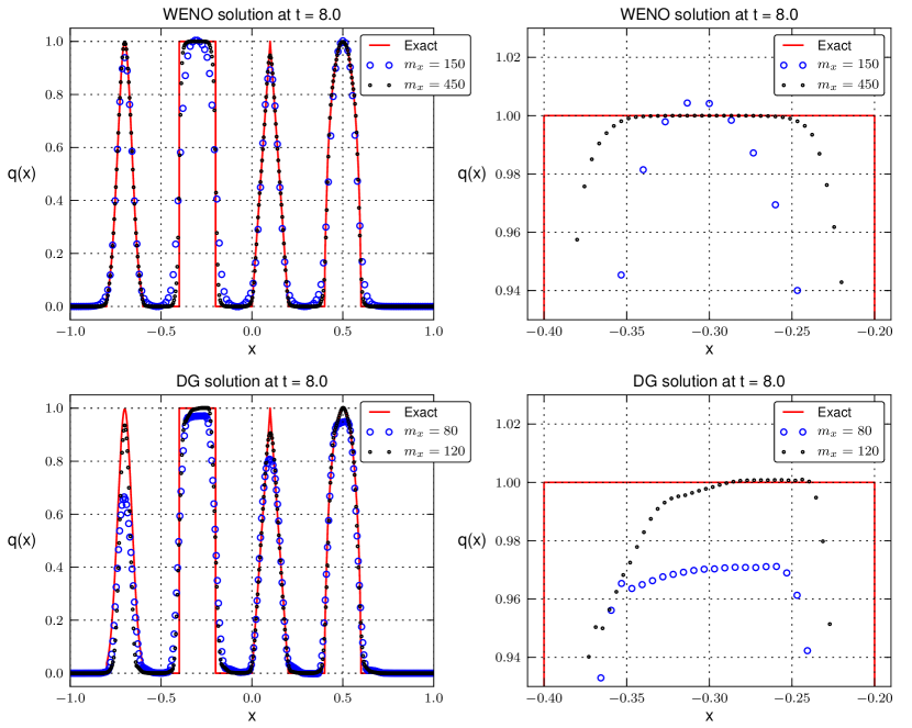
Results for this problem are presented in Figure 3. The under-resolved DG simulations tend to be quite diffusive when compared to the WENO schemes, but behave much more predictably.

Figure 3: Advection equation: a discontinuous example. Results for the two-derivative (TDRK4) method for WENO and DG spatial discretizations. Simulations are run to a final time of $t=8.0$ for a total of four full revolutions. The two images on the right are zoomed in images of the top of the square wave. WENO simulations use a CFL number of $\nu=0.4$, and the DG simulations use a constant CFL number of $\nu=0.08$. We again plot four points per cell for the DG solutions.

5.2 Buckley-Leverett

The Buckley-Leverett equation is a non-linear scalar problem with a non-convex flux function. Years past its invention, it has become a standard benchmark problem for many hyperbolic solvers. The model describes two-phase flow through porous media, where the application is oil recovery from a reservoir containing an oil-water or oil-gas mixture of fluids BuckLev42 . In rescaled units, the flux function for this problem is defined through a single free parameter $M$ with

$$f(q)=\frac{q^{2}}{q^{2}+M(1-q)^{2}}.$$ (79)

We use $M=1/3$, and we take the computational domain to be $[-1,1]$ with initial conditions prescribed through

$$q(0,x)=\begin{cases}1,\quad\text{if }-1/2\leq x\leq 0,\\ 0,\quad\text{otherwise}.\end{cases}$$ (80)

For small time values, the exact solution to this problem can be found by solving two Riemann problems, where each pair of states produces a typical ‘compound wave’ that is the combination of a leading shock and a trailing rarefaction. Each shock propagates with a speed dictated by the Rankine-Hugoniot conditions

$$f^{\prime}(q^{*})=\frac{f(q^{*})-f(q_{c})}{q^{*}-q_{c}},$$ (81)

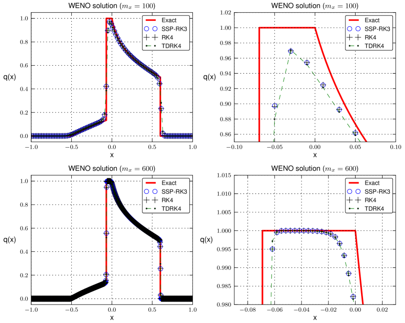
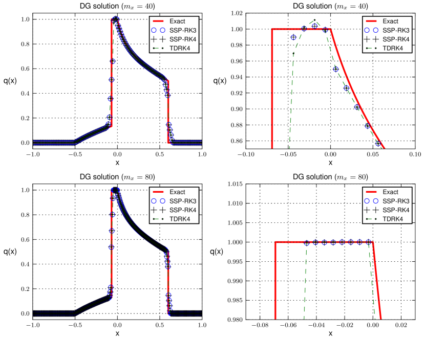
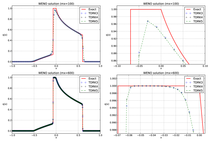
where $q_{c}$ is the constant value that does not change. For the Riemann problem located at $x=-0.5$, we have $q_{c}=1$, and $q^{*}\approx 0.1339745962155613$, and for the Riemann problem located at $x=0.0$, we have $q_{c}=0$ and $q^{*}=0.5$. Characteristics between $q^{*}$ and $q_{c}$ propagate with speed $f^{\prime}(q)$, and therefore to fill the rarefaction fan, we plot a range of values $(s+tf^{\prime}(q),q)$, where $q$ is a sampling of values between $q_{c}$ and $q^{*}$, and $s\in\left\{-0.5,0.0\right\}$ is the location of each Riemann problem. Results for the two spatial discretizations are presented in Figures 4 and 5 at a final time of $t=0.4$. In addition, we compare three different two-derivative methods that were presented in §2.3 in Figure 6.

As a final note, we remark that for this problem only, we modify our scheme to deal with some pathological issues. Given that the flux function is non-convex, the WENO simulations use the analytical value for $\alpha$, which is approximately $\alpha:=\max_{q\in[0,1]}|f^{\prime}(q)|\approx 2.205737062$. For the DG simulations, we use the HLL(E) Riemann solver HaLaLe83 . In this case, the HLL(E) solver performs better than the local Lax-Friedrichs (LLF) solver given that $f^{\prime}(q)\geq 0$ for all $q$ in our domain. The LLF solver approximates this problem with two waves traveling in opposite directions, whereas the exact solution travels in one direction only, which the HLL(E) correctly accounts for.

Figure 4: Buckley-Leverett double Riemann problem: WENO solutions. WENO results at the final time of $t=0.4$. All time integrators compared for this method are giving similar results. We remark that for this problem, the WENO schemes tend to be more diffusive where the rarefactions form when compared to the DG schemes.

Figure 5: Buckley-Leverett double Riemann problem: DG solutions. DG results at the final time of $t=0.4$. We plot exactly four uniformly spaced grid points per cell. The top row uses $m_{x}=40$ grid cells, and the bottom row uses $m_{x}=80$ grid cells. The two frames on the right are zoomed in images of the solution near $x=0.0$, one of the few places where we were able to find differences in the solutions. We note that the coarse solution is under resolved because it only has a single cell to capture the structure at the top of the solution. CFL numbers are chosen as in Table 6, which are close to the maximum stable time step allowed. All time integrators are qualitatively giving the same result.

Figure 6: Buckley-Leverett double Riemann problem: WENO solutions. WENO results at the final time of $t=0.4$. Here, we compare three different two-derivative methods that are presented in §2.3: TDRK3 (16), TDRK4 (18) and TDRK5 (17). The only noticeable difference is given by the third-order scheme, and we attribute this to the lower order temporal accuracy.

5.3 Shallow water

The shallow water equations define a hyperbolic system with two conserved quantities: the water height $h$, and velocity $u$. The system is defined by

$$\left(\begin{array}[]{c}h\\ hu\end{array}\right)_{,t}+\left(\begin{array}[]{c}hu\\ hu^{2}+\frac{1}{2}gh^{2}\end{array}\right)_{,x}=0.$$ (86)

For our simulation, we take $g=1$. We demonstrate our method on the dam break Riemann problem bLe02 with initial conditions defined by

$$(h,u)^{T}=\begin{cases}(3,0)^{T},\quad\text{if }x\leq 0.5,\\ (1,0)^{T},\quad\text{otherwise}.\end{cases}$$ (87)

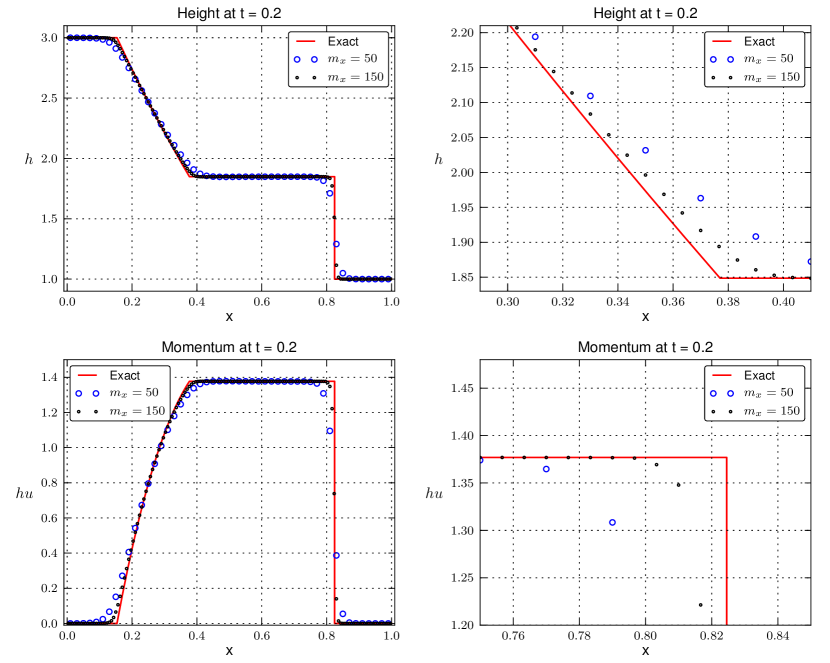
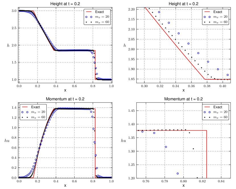
We use a computational domain of $[0,1]$ with outflow boundary conditions, and stop the simulation at a final time of $t=0.2$. Results for the two-derivative time integrators are presented in Figure 7 for the WENO method, and in Figure 8 for the discontinuous Galerkin scheme. Exact solutions for this problem can be found in textbooks bLe02 .

Figure 7: Shallow water Riemann problem: WENO solutions. Here we present two resolutions on top of each other using the new multiderivative scheme presented in §3.2. We use $m_{x}=50$ points for a coarse resolution and $m_{x}=150$ points for a finer solution. Top row: water height $h$ at the final time with a zoom in of the rarefaction to the right. Bottom row: momentum $hu$, with a zoom in of the shock to the right.

Figure 8: Shallow water Riemann problem: DG solutions. Here we present two resolutions on top of each other using the new multiderivative scheme presented in §4.2. We use $m_{x}=20$ cells for a coarse resolution and $m_{x}=60$ cells for a finer solution, and we plot exactly four uniformly spaced points per cell. Top row: water height $h$ at the final time with a zoom in of the rarefaction to the right. Bottom row: momentum $hu$, with a zoom in of the shock to the right.

5.4 Euler equations

The Euler equations describe the evolution of density $\rho$, momentum $\rho u$ and energy $\mathcal{E}$ of an ideal gas:

$$\left(\begin{array}[]{c}\rho\\ \rho u\\ \mathcal{E}\end{array}\right)_{,t}+\left(\begin{array}[]{c}\rho u\\ \rho u^{2}+p\\ (\mathcal{E}+p)u\end{array}\right)_{,x}=0,$$ (94)

where $p$ is the pressure. The energy $\mathcal{E}$ is related to the primitive variables $\rho$, $u$ and $p$ by

$$\mathcal{E}=\frac{p}{\gamma-1}+\frac{1}{2}\rho u^{2},$$ (95)

where $\gamma$ is the ratio of specific heats. For all of our simulations, we take $\gamma=1.4$.

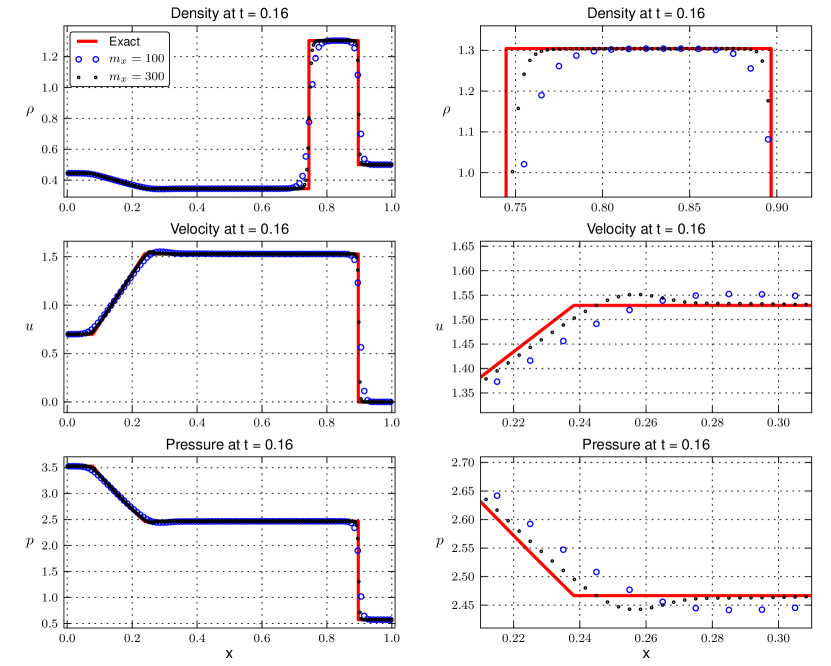
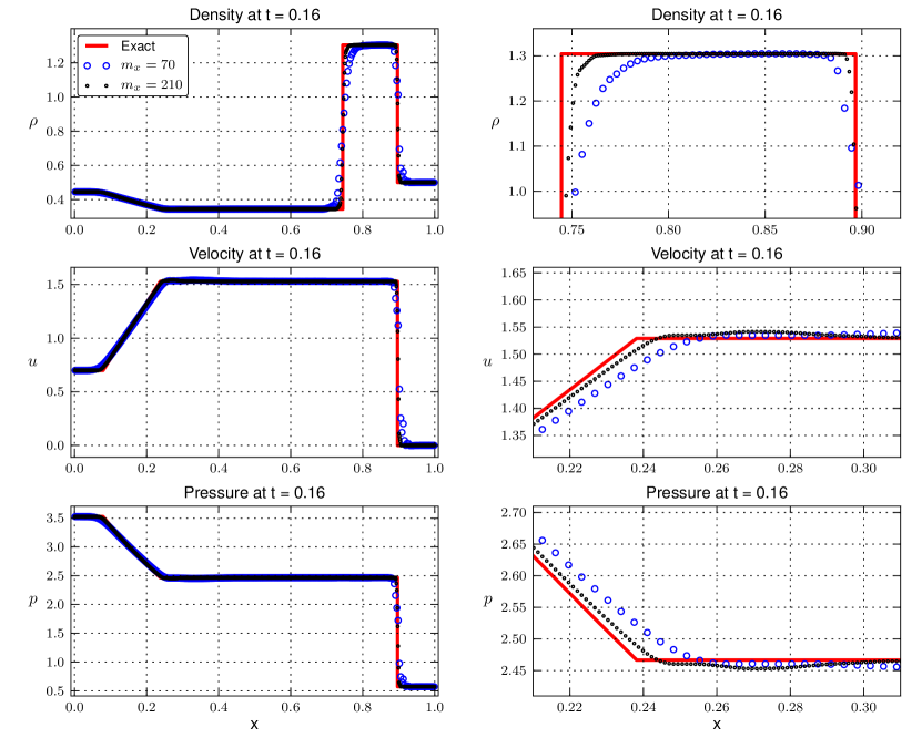
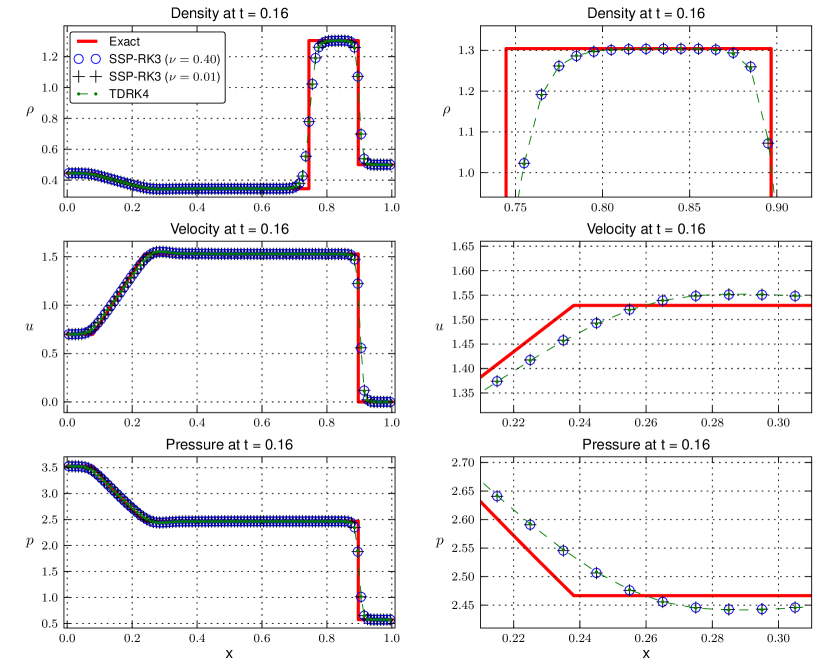
5.4.1 Euler equations: a shock tube Riemann problem

We present a classic test case of a difficult shock tube, which is commonly referred to as the Lax shock tube. The initial conditions are those defined by Harten Harten78 ; HaEnOsCh87 :

$$(\rho,\rho u,\mathcal{E})^{T}=\begin{cases}(0.445,0.3111,8.928)^{T},\quad\text{if }x\leq 0.5,\\ (0.5,0,1.4275)^{T},\quad\text{otherwise}.\end{cases}$$ (96)

Exact solutions for this problem are well understood, and there are many textbooks that describe how to construct them bLe02 ; Toro99 . For this set of data, the solution contains a left rarefaction, a contact discontinuity and a shock wave traveling to the right.

We select $t=0.16$ for the final time of our simulation QiuShu03 , and we use a computational domain of $[0,1]$ with outflow boundary conditions. Results for this problem are presented in Figures 9 and 10. For the WENO simulations, we additionally compare the two-derivative two-derivative time integrator TDRK4 against the SSP-RK3 with two different CFL numbers, $\nu=0.01$ and then $\nu=0.4$. We present results for the time integrator comparison in Figure 11.

Figure 9: Shock-tube Riemann problem: WENO solutions. Shown here are WENO simulations with Harten’s initial conditions (96) for the shock tube problem. We plot observable quantities from top to bottom: density $\rho$, velocity $u$, and pressure $p$. Left columns are the full solution, and right columns are zoomed in parts of the same data points. We present a coarse solution with $m_{x}=100$ points and a finer solution of $m_{x}=300$ points. The zoomed in image of the density indicates the top part of the square section between the contact discontinuity and the right traveling shock. The zoomed in images for the velocity and pressure focus in on the right foot of the rarefaction fan.

Figure 10: Shock-tube Riemann problem: DG solutions. We present two DG simulations for the physical observables, which from top to bottom are: density $\rho$, velocity $u$, and pressure $p$. Left columns are the full solution, and right columns are zoomed in parts of the same data points. We present a coarse solution with $m_{x}=70$ grid cells and a finer solution of $m_{x}=210$ grid cells, and we plot four uniformly spaced points per cell. The axes are identical to those in Figure 9.

Figure 11: Shock-tube Riemann problem: WENO solutions. Shown here are WENO simulations comparing two different time integrators: the third-order SSP method of Osher and Shu against the new two-stage, two-derivative method (TDRK4). We repeat that all WENO simulations with the TDRK4 time integrator use a CFL number of $\nu=0.4$. Here, we observe that the third-order SSP method with CFL numbers of $\nu=0.4$ and $\nu=0.01$ behaves qualitatively the same as the TDRK4 method. We plot observable quantities from top to bottom: density $\rho$, velocity $u$, and pressure $p$. Left columns are the full solution, and right columns are zoomed in parts of the same data points. The resolution for this picture is the coarse solution of $m_{x}=100$ identical to the coarse solution used in Figure 9. Again, we remark that the accepted time integrator is in close agreement with the proposed method.

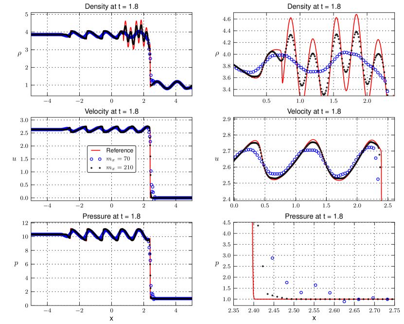
5.4.2 Euler equations: shock entropy

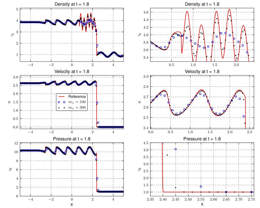
Our final test case is another problem that is popular in the literature ShuOsher89 . The initial conditions are

$$(\rho,u,p)= \left(3.857143,2.629369,10.3333\right),\quad x<-4,$$

$$(\rho,u,p)= \left(1+\epsilon\sin(5x),0,1\right),\quad x\geq-4,$$

with a computational domain of $[-5,5]$. The final time for this simulation is $t=1.8$. With $\epsilon=0$, this is a pure Mach 3 shock moving to the right. We follow the common practice of setting $\epsilon=0.2$.

Results for WENO simulations are presented in Figure 12, and DG results are presented in Figure 13. For a reference solution, we plot a WENO simulation that uses the SSP-RK3 method described in Gottlieb and Shu GoShu98 , with $m_{x}=6000$ points and a small CFL number of $\nu=0.1$.

Figure 12: Shock-entropy: WENO solutions. Shown here are WENO solutions to the shock-entropy interaction problem presented in §5.4.2. We plot observable quantities from top to bottom: density $\rho$, velocity $u$, and pressure $p$. Left columns are the full solution, and right columns are zoomed in parts of the same data points. We present a coarse solution with $m_{x}=100$ points and a finer solution of $m_{x}=300$ points.

Figure 13: Shock entropy. Shown here are DG solutions to the shock-entropy interaction problem presented in §5.4.2. We use a coarse mesh of $m_{x}=70$ and a finer mesh of $m_{x}=210$. The reference solution is identical to the one used in Figure 12 that is a WENO simulation with $6000$ points, and CFL number of $\nu=0.1$ with the third-order SSP-RK3 time integrator. Again, the DG schemes tend to be more diffusive on this problem when compared to the WENO method, and the limiter used in this work tends to clip the peaks for the coarse resolutions. We repeat that we are plotting exactly four points per cell, and therefore, the observable oscillations for the coarse resolution are happening on a sub-cell level. Although not shown, plots of cell averages only do not visibly demonstrate these oscillations. Results for other time integrators are found to be comparable.

6 Conclusions and future work

We have presented a family of methods that generalize popular high-order time integration methods for hyperbolic conservation laws. The explicit multistage multiderivative (multiderivative Runge-Kutta) time integrators that are the subject of this work provide the ability to access to higher temporal derivatives for an explicit (single-derivative) Runge-Kutta method, and they introduce degrees of freedom by adding stages to high-order (single-stage) Taylor methods. Numerous numerical examples were presented that included multiderivative schemes for high-order discontinuous Galerkin and WENO methods. In order to implement the multiderivative technology, we leveraged recent work on Lax-Wendroff type time integrators for the two aforementioned spatial discretizations investigated; each method required a very different procedure for defining the higher derivatives. Numerical results for the new multiderivative schemes are promising: they are demonstrably comparable to those obtained from popular high-order SSP integrators, they introduce greater portability to high-order Lax-Wendroff methods, and they decrease the memory footprint for Runge-Kutta methods by introducing higher time derivatives.

Future work will focus on extensions to higher dimensions, as well as a mathematical exploration into the numerical properties of multiderivative schemes for PDEs. In addition, an investigation into the optimization of these methods for modern computer architectures such as graphics processing units (GPUs) should be conducted. This will include implementation and timing comparison tests of these methods on GPUs. We would like to explore developing multiderivative methods with SSP properties, as well as low-storage ‘many’-stage variations of the two-derivative method presented in this work. Additionally, we would like to investigate implicit and explicit multistage multiderivative methods for solving parabolic partial differential equations.