MUSIC for Faraday Rotation Measure Synthesis

M. Andrecut
Institute for Space Imaging Science, University of Calgary, Calgary, Alberta, T2N 1N4, Canada
E-mail: mandrecu@ucalgary.ca; mircea.andrecut@gmail.com
(Accepted 1988 December 15. Received 1988 December 14; in original form 2012 October 15)
Abstract

Faraday Rotation Measure (RM) synthesis requires the recovery of the Faraday Dispersion Function (FDF) from measurements restricted to limited wavelength ranges, which is an ill-conditioned deconvolution problem. Here, we propose a novel deconvolution method based on an extension of the MUltiple SIgnal Classification (MUSIC) algorithm. The complexity and speed of the method is determined by the eigen-decomposition of the covariance matrix of the observed polarizations. We show numerically that for high to moderate Signal to Noise (S/N) cases the RM-MUSIC method is able to recover the Faraday depth values of closely spaced pairs of thin RM components, even in situations where the peak response of the FDF is outside of the RM range between the two input RM components. This result is particularly important because the standard deconvolution approach based on RM-CLEAN fails systematically in such situations, due to its greedy mechanism used to extract the RM components. For low S/N situations, both the RM-MUSIC and RM-CLEAN methods provide similar results.

keywords:
data analysis - Techniques: polarimetric - magnetic fields
pagerange: MUSIC for Faraday Rotation Measure SynthesisMUSIC for Faraday Rotation Measure Synthesispubyear: 2002

1 Introduction

Faraday rotation is a physical phenomenon where the position angle of linearly polarized radiation propagating through a magneto-ionic medium is rotated as a function of frequency. Faraday Rotation Measure (RM) synthesis is an important method for analyzing multichannel polarized radio data, where multiple emitting regions are present along the single line of sight of the observations (Brentjens & de Bruyn, 2005). In practice, the method requires the recovery of the Faraday Dispersion Function (FDF) from measurements restricted to limited wavelength ranges, which is an ill-conditioned deconvolution problem, raising important computational difficulties. At least four different approaches have been proposed so far to solve this problem. A first approach uses an adaptation of the CLEAN algorithm (Hogbom, 1974) to the RM deconvolution (RM-CLEAN) (Heald et al., 2009). The second approach is wavelet-based, and assumes field symmetries in order to project the observed data onto λ2<0superscript𝜆20\lambda^{2}<0 (Frick et al., 2010). The third approach relies on nonlinear model fitting (Farnsworth et al., 2011), while the fourth approach is based on the novel compressed sensing (CS) paradigm (Li et al., 2011; Andrecut et al., 2012). Whether these methods are successful or not in detecting the structure of the FDF depends on the Signal to Noise ratio (S/N), the separation of the RM components, the relative angle of the RM components at the observed wavelengths, and the wavelength range. For example, the current existing methods fail to recover the correct RM components when the separation among them is below the resolution determined from the half maximum of the main peak of the RM spread function (RMSF). Also, another major problem is related to situations where the interference of pairs of RM components conspire to place the peak response of the FDF outside of the RM range between the two input RM components. In this case, the standard RM-CLEAN method fails, due to its intrinsic greedy mechanism used to pick up the RM components. Here we discuss a novel approach, which addresses these two significant problems from a different perspective. The proposed method is an extension of the MUltiple SIgnal Classification (MUSIC) algorithm, which is based on the eigen-decomposition (ED) of the covariance matrix of the observed data (Cheney, 2001). The complexity and the speed of the method is therefore determined by the size of the eigen-decomposition problem, which for several hundreds of data points is comparable to the RM-CLEAN approach. Our numerical results show that for high to moderate S/N cases, the RM-MUSIC method gives very good results, outperforming the standard approach based on RM-CLEAN. For low S/N situations, both the RM-MUSIC and RM-CLEAN methods provide similar results. We should note that contrary to the other existing methods, the RM-MUSIC method recovers only the Faraday depth values. Once the Faraday depth values are determined, the real and imaginary parts of the RM components can be easily computed using the linear least squares fitting approach.

2 RM-Synthesis

The Faraday depth (in radm2radsuperscriptm2\mathrm{rad}\,\mathrm{m}^{-2}) is defined as:

ϕ(r)=0.81sourceobserverne𝐁𝐝𝐫,italic-ϕ𝑟0.81superscriptsubscript𝑠𝑜𝑢𝑟𝑐𝑒𝑜𝑏𝑠𝑒𝑟𝑣𝑒𝑟subscript𝑛𝑒𝐁𝐝𝐫\phi(r)=0.81\int_{source}^{observer}n_{e}\mathbf{B}\cdot\mathbf{dr}, (1)

where nesubscript𝑛𝑒n_{e} is the electron density (in cm3𝑐superscript𝑚3cm^{-3}) , B𝐵B is the magnetic field (in μG𝜇𝐺\mu G), and dr𝑑𝑟dr is the infinitesimal path length (in parsecs). We also define the complex polarization as:

P(λ2)=Q(λ2)+iU(λ2)=pIe2iχ(λ2),𝑃superscript𝜆2𝑄superscript𝜆2𝑖𝑈superscript𝜆2𝑝𝐼superscript𝑒2𝑖𝜒superscript𝜆2P(\lambda^{2})=Q(\lambda^{2})+iU(\lambda^{2})=pIe^{2i\chi(\lambda^{2})}, (2)

where p𝑝p is the fractional polarization, I𝐼I, Q𝑄Q, U𝑈U are the observed Stokes parameters, and χ(λ2)𝜒superscript𝜆2\chi(\lambda^{2}) is the polarization angle observed at wavelength λ𝜆\lambda. Also, we assume that the observed polarization P(λ2)𝑃superscript𝜆2P(\lambda^{2}) originates from the emission at all possible values of ϕitalic-ϕ\phi, corresponding to the Fourier transform:

P(λ2)=+F(ϕ)e2iϕλ2𝑑ϕ,𝑃superscript𝜆2superscriptsubscript𝐹italic-ϕsuperscript𝑒2𝑖italic-ϕsuperscript𝜆2differential-ditalic-ϕP(\lambda^{2})=\int_{-\infty}^{+\infty}F(\phi)e^{2i\phi\lambda^{2}}d\phi, (3)

where F(ϕ)𝐹italic-ϕF(\phi) is the complex FDF (the intrinsic polarized flux, as a function of the Faraday depth). Thus, in principle F(ϕ)𝐹italic-ϕF(\phi) is the inverse Fourier transform of the observed quantity P(λ2)𝑃superscript𝜆2P(\lambda^{2}):

F(ϕ)=+P(λ2)e2iϕλ2𝑑λ2.𝐹italic-ϕsuperscriptsubscript𝑃superscript𝜆2superscript𝑒2𝑖italic-ϕsuperscript𝜆2differential-dsuperscript𝜆2F(\phi)=\int_{-\infty}^{+\infty}P(\lambda^{2})e^{-2i\phi\lambda^{2}}d\lambda^{2}. (4)

However, this operation is ill-defined since we cannot observe P(λ2)𝑃superscript𝜆2P(\lambda^{2}) for λ2<0superscript𝜆20\lambda^{2}<0, and also in general the observations are limited to an interval [λmin2,λmax2]superscriptsubscript𝜆𝑚𝑖𝑛2superscriptsubscript𝜆𝑚𝑎𝑥2[\lambda_{min}^{2},\lambda_{max}^{2}].

In order to deal with the above limitations, the observed polarization is defined as:

P~(λ2)=W(λ2)P(λ2),~𝑃superscript𝜆2𝑊superscript𝜆2𝑃superscript𝜆2\tilde{P}(\lambda^{2})=W(\lambda^{2})P(\lambda^{2}), (5)

where W𝑊W is the observation window function, with W(λ2)>0𝑊superscript𝜆20W(\lambda^{2})>0 for λ2[λmin2,λmax2]superscript𝜆2superscriptsubscript𝜆𝑚𝑖𝑛2superscriptsubscript𝜆𝑚𝑎𝑥2\lambda^{2}\in[\lambda_{min}^{2},\lambda_{max}^{2}], and W(λ2)=0𝑊superscript𝜆20W(\lambda^{2})=0 otherwise. Therefore, for N𝑁N measurement channels with frequencies νnsubscript𝜈𝑛\nu_{n}, wavelengths λn=c/νnsubscript𝜆𝑛𝑐subscript𝜈𝑛\lambda_{n}=c/\nu_{n}, n=1,2,,N𝑛12𝑁n=1,2,...,N (c𝑐c is the speed of light), weights W(λn2)=Wn𝑊superscriptsubscript𝜆𝑛2subscript𝑊𝑛W(\lambda_{n}^{2})=W_{n}, polarizations P(λn2)=Pn𝑃superscriptsubscript𝜆𝑛2subscript𝑃𝑛P(\lambda_{n}^{2})=P_{n}, we obtain the following discrete expression for the FDF:

F(ϕ)=A1n=0N1WnPne2iϕ(λn2λr2),𝐹italic-ϕsuperscript𝐴1superscriptsubscript𝑛0𝑁1subscript𝑊𝑛subscript𝑃𝑛superscript𝑒2𝑖italic-ϕsuperscriptsubscript𝜆𝑛2superscriptsubscript𝜆𝑟2F(\phi)=A^{-1}\sum_{n=0}^{N-1}W_{n}P_{n}e^{-2i\phi(\lambda_{n}^{2}-\lambda_{r}^{2})}, (6)

where

A=[n=0N1Wn]1𝐴superscriptdelimited-[]superscriptsubscript𝑛0𝑁1subscript𝑊𝑛1A=\left[\sum_{n=0}^{N-1}W_{n}\right]^{-1} (7)

is a normalization constant, and the reference wavelength λr2superscriptsubscript𝜆𝑟2\lambda_{r}^{2} is defined as:

λr2=A1n=0N1Wnλn2.superscriptsubscript𝜆𝑟2superscript𝐴1superscriptsubscript𝑛0𝑁1subscript𝑊𝑛superscriptsubscript𝜆𝑛2\lambda_{r}^{2}=A^{-1}\sum_{n=0}^{N-1}W_{n}\lambda_{n}^{2}. (8)

In our approach we assume that the model of F(ϕ)𝐹italic-ϕF(\phi) contains KNmuch-less-than𝐾𝑁K\ll N (unknown) components fkδ(ϕϕk)subscript𝑓𝑘𝛿italic-ϕsubscriptitalic-ϕ𝑘f_{k}\delta(\phi-\phi_{k}), where fksubscript𝑓𝑘f_{k} are complex and ϕksubscriptitalic-ϕ𝑘\phi_{k} are real quantities k=0,,K1𝑘0𝐾1k=0,...,K-1:

F(ϕ)=k=0K1fkδ(ϕϕk).𝐹italic-ϕsuperscriptsubscript𝑘0𝐾1subscript𝑓𝑘𝛿italic-ϕsubscriptitalic-ϕ𝑘F(\phi)=\sum_{k=0}^{K-1}f_{k}\delta(\phi-\phi_{k}). (9)

Considering additive noise in the measurement process, the sampled polarization-domain channel response is given by:

Pn=Wnk=1Kfke2iϕk(λn2λr2)+αn+iβn,n=1,2,,N,formulae-sequencesubscript𝑃𝑛subscript𝑊𝑛superscriptsubscript𝑘1𝐾subscript𝑓𝑘superscript𝑒2𝑖subscriptitalic-ϕ𝑘superscriptsubscript𝜆𝑛2superscriptsubscript𝜆𝑟2subscript𝛼𝑛𝑖subscript𝛽𝑛𝑛12𝑁P_{n}=W_{n}\sum_{k=1}^{K}f_{k}e^{2i\phi_{k}(\lambda_{n}^{2}-\lambda_{r}^{2})}+\alpha_{n}+i\beta_{n},\quad n=1,2,...,N, (10)

where N𝑁N is the number of measured channels. Here, both αnsubscript𝛼𝑛\alpha_{n} and βnsubscript𝛽𝑛\beta_{n} are Gaussian variables with mean zero and standard deviation σ𝜎\sigma. Obviously, F(ϕ)𝐹italic-ϕF(\phi) is a “dirty” reconstruction, and a deconvolution step is necessary to recover the RM components fkδ(ϕϕk)subscript𝑓𝑘𝛿italic-ϕsubscriptitalic-ϕ𝑘f_{k}\delta(\phi-\phi_{k}), given the observed values Pnsubscript𝑃𝑛P_{n} and the weights Wnsubscript𝑊𝑛W_{n}.

3 RM-MUSIC

The MUSIC method is generally used for estimating frequencies in signal processing problems, and the location of pointlike scatterers in imaging problems (see Cheney (2001) for a review). The standard MUSIC method is based on the ED of an Hermitian operator, which corresponds to the covariance matrix of the signal or the array response matrix. By the finite-dimensional spectral theorem, such operators can be associated with an orthonormal basis of the underlying space in which the operator is represented as a diagonal matrix with real number entries. The main idea is to estimate the frequencies, or to localize multiple sources, by exploiting the eigen-structure of this Hermitian operator. More exactly the space spanned by its eigenvectors can be partitioned into two orthogonal subspaces, namely the signal subspace and the noise subspace. By exploiting the orthogonality of the signal and noise subspaces, the MUSIC method significantly improves the resolution (i.e. locating closely spaced frequencies or scatterers), and as a consequence it is considered a super-resolution method. Let us now formulate the standard MUSIC approach to the Faraday depth recovery problem.

Since only one snapshot of measurement data P𝑃P of length N𝑁N is available, the data sequence is divided into M=NL𝑀𝑁𝐿M=N-L segments of length L𝐿L, 0<LN0𝐿𝑁0<L\leq N, and then the L×L𝐿𝐿L\times L covariance matrix is estimated as:

𝐆^=1Mm=0M1𝐏(m)(𝐏(m))H^𝐆1𝑀superscriptsubscript𝑚0𝑀1superscript𝐏𝑚superscriptsuperscript𝐏𝑚𝐻\mathbf{\hat{G}}=\frac{1}{M}\sum_{m=0}^{M-1}\mathbf{P}^{(m)}(\mathbf{P}^{(m)})^{H} (11)

where 𝐏(m)=[Pm,Pm+1,,Pm+L]Tsuperscript𝐏𝑚superscriptsubscript𝑃𝑚subscript𝑃𝑚1subscript𝑃𝑚𝐿𝑇\mathbf{P}^{(m)}=[P_{m},P_{m+1},...,P_{m+L}]^{T}, m=0,1,,M1𝑚01𝑀1m=0,1,...,M-1, and the superscript H𝐻H denotes the conjugate transpose operation. Suppose that μ0μ1μL1\mu_{0}\geq\mu{}_{1}\geq...\geq\mu{}_{L-1} and 𝐠(0),𝐠(1),,𝐠(L1)superscript𝐠0superscript𝐠1superscript𝐠𝐿1\mathbf{g}^{(0)},\mathbf{g}^{(1)},...,\mathbf{g}^{(L-1)} are the eivenvalues, and respectively the eigenvectors of 𝐆^^𝐆\mathbf{\hat{G}}, such that:

𝐆^𝐠()=μ𝐠(),^𝐆superscript𝐠subscript𝜇superscript𝐠\mathbf{\hat{G}}\mathbf{g}^{(\ell)}=\mu_{\ell}\mathbf{g}^{(\ell)}, (12)

and

𝐆^==0L1μ𝐠()(𝐠())H.^𝐆superscriptsubscript0𝐿1subscript𝜇superscript𝐠superscriptsuperscript𝐠𝐻\mathbf{\hat{G}}=\sum_{\ell=0}^{L-1}\mu_{\ell}\mathbf{g}^{(\ell)}(\mathbf{g}^{(\ell)})^{H}. (13)

Since the measured signal contains only K𝐾K components, the last LK𝐿𝐾L-K eigenvalues of 𝐆^^𝐆\mathbf{\hat{G}}, μKμK+1μL1subscript𝜇𝐾subscript𝜇𝐾1subscript𝜇𝐿1\mu_{K}\geq\mu_{K+1}\geq...\geq\mu_{L-1}, should be small and below the noise level, and we say that the corresponding eigenvectors 𝐠(K),𝐠(K+1),,𝐠(L1)superscript𝐠𝐾superscript𝐠𝐾1superscript𝐠𝐿1\mathbf{g}^{(K)},\mathbf{g}^{(K+1)},...,\mathbf{g}^{(L-1)} span the noise subspace of 𝐆^^𝐆\mathbf{\hat{G}}, while the first K𝐾K eigenvectors 𝐠(0),𝐠(1),,𝐠(K1)superscript𝐠0superscript𝐠1superscript𝐠𝐾1\mathbf{g}^{(0)},\mathbf{g}^{(1)},...,\mathbf{g}^{(K-1)} span the signal subspace, and the corresponding eigenvalues and eigenvalues μ0μ1μK1\mu_{0}\geq\mu{}_{1}\geq...\geq\mu{}_{K-1} should be above the noise level. Thus, the eigen-decomposition of 𝐆^^𝐆\mathbf{\hat{G}} can be written as:

𝐆^==0K1μ𝐠()(𝐠())Hsignalsubspace+=KL1μ𝐠()(𝐠())Hnoisesubspace.^𝐆subscriptsuperscriptsubscript0𝐾1subscript𝜇superscript𝐠superscriptsuperscript𝐠𝐻𝑠𝑖𝑔𝑛𝑎𝑙𝑠𝑢𝑏𝑠𝑝𝑎𝑐𝑒subscriptsuperscriptsubscript𝐾𝐿1subscript𝜇superscript𝐠superscriptsuperscript𝐠𝐻𝑛𝑜𝑖𝑠𝑒𝑠𝑢𝑏𝑠𝑝𝑎𝑐𝑒\mathbf{\hat{G}}=\underbrace{\sum_{\ell=0}^{K-1}\mu_{\ell}\mathbf{g}^{(\ell)}(\mathbf{g}^{(\ell)})^{H}}_{signal\,subspace}+\underbrace{\sum_{\ell=K}^{L-1}\mu_{\ell}\mathbf{g}^{(\ell)}(\mathbf{g}^{(\ell)})^{H}}_{noise\,subspace}. (14)

We can now form the projection operator onto the noise subspace defined as:

𝐆^𝐠(noise)==KL1𝐠()(𝐠())H,superscriptsubscript^𝐆𝐠𝑛𝑜𝑖𝑠𝑒superscriptsubscript𝐾𝐿1superscript𝐠superscriptsuperscript𝐠𝐻\mathbf{\hat{G}}_{\mathbf{g}}^{(noise)}=\sum_{\ell=K}^{L-1}\mathbf{g}^{(\ell)}(\mathbf{g}^{(\ell)})^{H}, (15)

and consider the signal subspace sampling vector

𝐡(ϕ~)=[e2iϕ~λ~02,e2iϕ~λ~12,,e2iϕ~λ~L12]T,\mathbf{h}(\tilde{\phi})=[e^{2i\tilde{\phi}\tilde{\lambda}{}_{0}^{2}},e^{2i\tilde{\phi}\tilde{\lambda}{}_{1}^{2}},...,e^{2i\tilde{\phi}\tilde{\lambda}{}_{L-1}^{2}}]^{T}, (16)

where the wavelengths are interpolated as following:

λ~=2[cνNL1(νNν1)]2,=0,1,,L1,\tilde{\lambda}{}_{\ell}^{2}=\left[\frac{c}{\nu_{N}-\frac{\ell}{L-1}(\nu_{N}-\nu_{1})}\right]^{2},\quad\ell=0,1,...,L-1, (17)

such that they cover the initial observation interval [λmin,λmax]subscript𝜆𝑚𝑖𝑛subscript𝜆𝑚𝑎𝑥[\lambda_{min},\lambda_{max}] We should note that since LN𝐿𝑁L\leq N, the Faraday depth is also linearly interpolated as ϕ~=ϕL/N~italic-ϕitalic-ϕ𝐿𝑁\tilde{\phi}=\phi L/N, and therefore we obtain:

𝐡(ϕ)=[e2iLNϕλ~02,e2iLNϕλ~12,,e2iLNϕλ~L12]T.\mathbf{h}(\phi)=[e^{2i\frac{L}{N}\phi\tilde{\lambda}{}_{0}^{2}},e^{2i\frac{L}{N}\phi\tilde{\lambda}{}_{1}^{2}},...,e^{2i\frac{L}{N}\phi\tilde{\lambda}{}_{L-1}^{2}}]^{T}. (18)

If the vector 𝐡(ϕ)𝐡italic-ϕ\mathbf{h}(\phi) represents the signal, i.e. it is a linear combination of the signal subspace eigenvectors, then its projection onto the noise subspace must be close to zero:

𝐆^𝐠(noise)𝐡(ϕ)0.similar-to-or-equalsnormsuperscriptsubscript^𝐆𝐠𝑛𝑜𝑖𝑠𝑒𝐡italic-ϕ0\left\|\mathbf{\hat{G}}_{\mathbf{g}}^{(noise)}\mathbf{h}(\phi)\right\|\simeq 0. (19)

Thus, the Faraday depth values ϕksubscriptitalic-ϕ𝑘\phi_{k}, k=0,1,,K1𝑘01𝐾1k=0,1,...,K-1, should correspond to the maxima of the following MUSIC pseudo-spectrum:

S(ϕ)=1𝐆^𝐠(noise)𝐡(ϕ)2=1=KL1(𝐠())H𝐡(ϕ)2.𝑆italic-ϕ1superscriptnormsuperscriptsubscript^𝐆𝐠𝑛𝑜𝑖𝑠𝑒𝐡italic-ϕ21superscriptsubscript𝐾𝐿1superscriptnormsuperscriptsuperscript𝐠𝐻𝐡italic-ϕ2S(\phi)=\frac{1}{\left\|\mathbf{\hat{G}}_{\mathbf{g}}^{(noise)}\mathbf{h}(\phi)\right\|^{2}}=\frac{1}{\sum_{\ell=K}^{L-1}\left\|(\mathbf{g}^{(\ell)})^{H}\mathbf{h}(\phi)\right\|^{2}}. (20)

Once the Faraday depth values ϕksubscriptitalic-ϕ𝑘\phi_{k} are determined from the MUSIC pseudo-spectrum the real and imaginary parts of the RM components fksubscript𝑓𝑘f_{k} can be easily computed using the linear least squares fitting approach, i.e. by solving the following minimization problem:

{fk}k=0K1=argminfkn=0N1[Pnk=1Kfke2iϕkλn2]2superscriptsubscriptsubscript𝑓𝑘𝑘0𝐾1subscriptsubscript𝑓𝑘superscriptsubscript𝑛0𝑁1superscriptdelimited-[]subscript𝑃𝑛superscriptsubscript𝑘1𝐾subscript𝑓𝑘superscript𝑒2𝑖subscriptitalic-ϕ𝑘superscriptsubscript𝜆𝑛22\{f_{k}\}_{k=0}^{K-1}=\arg\min_{f_{k}}\sum_{n=0}^{N-1}\left[P_{n}-\sum_{k=1}^{K}f_{k}e^{2i\phi_{k}\lambda_{n}^{2}}\right]^{2}
=argmin𝐟𝐏𝚿^𝐟.absentsubscript𝐟norm𝐏^𝚿𝐟=\arg\min_{\mathbf{f}}\left\|\mathbf{P}-\hat{\mathbf{\mathbf{\Psi}}}\mathbf{f}\right\|. (21)

This least-squares fit problem has fewer free parameters, and it is far better constrained than the fit that would have been done without MUSIC. In fact the problem has an unique minimum norm solution, obtained by solving the linear system of equations: 𝚿^𝐟=𝐏^𝚿𝐟𝐏\mathbf{\hat{\mathbf{\Psi}}}\mathbf{f}=\mathbf{P}, where 𝐟=[f0,f1,,fK1]T𝐟superscriptsubscript𝑓0subscript𝑓1subscript𝑓𝐾1𝑇\mathbf{f}=[f_{0},f_{1},...,f_{K-1}]^{T} are the unknown components, 𝐏=[P0,P1,,PN1]T𝐏superscriptsubscript𝑃0subscript𝑃1subscript𝑃𝑁1𝑇\mathbf{P}=[P_{0},P_{1},...,P_{N-1}]^{T} are the observed polarizations, and 𝚿^^𝚿\hat{\mathbf{\mathbf{\Psi}}} is the Fourier matrix with the elements Ψn,k=e2iϕkλn2subscriptΨ𝑛𝑘superscript𝑒2𝑖subscriptitalic-ϕ𝑘superscriptsubscript𝜆𝑛2\Psi_{n,k}=e^{2i\phi_{k}\lambda_{n}^{2}}. Thus, the least squares solution is given by 𝐟=𝚿^𝐏𝐟superscript^𝚿𝐏\mathbf{f}=\hat{\mathbf{\mathbf{\Psi}}}^{\dagger}\mathbf{P}, where 𝚿^=(𝚿^H𝚿^)1𝚿^Hsuperscript^𝚿superscriptsuperscript^𝚿𝐻^𝚿1superscript^𝚿𝐻\hat{\mathbf{\mathbf{\Psi}}}^{\dagger}=(\hat{\mathbf{\mathbf{\Psi}}}^{H}\hat{\mathbf{\mathbf{\Psi}}})^{-1}\hat{\mathbf{\mathbf{\Psi}}}^{H} is the Moore-Penrose pseudo-inverse of 𝚿^^𝚿\hat{\mathbf{\mathbf{\Psi}}}.

4 Numerical Implementation

In order to optimally use the MUSIC method we also need to determine the number of components K𝐾K in the polarization signal. In principle, K𝐾K can be determined from the eigenvalues of the covariance matrix. The first largest eigenvalues, which are much bigger than the noise level μ>σ2subscript𝜇superscript𝜎2\mu_{\ell}>\sigma^{2}, =0,1,K101𝐾1\ell=0,1,...K-1, should indicate the value of K𝐾K. However, in a practical implementation, when the covariance matrix is estimated from a small number of observations, it is challenging to clearly separate the signal eigenvalues from the noise eigenvalues. In these ambiguous cases one can use information theoretic criteria for selection, like the Minimum Descriptive Length (MDL) criteria, where the value of K𝐾K corresponds to the minimum of the following quantity:

H(K)=M(MK)log(m=KMμm1/(MK)1MKm=KMμm)𝐻𝐾𝑀𝑀𝐾superscriptsubscriptproduct𝑚𝐾𝑀superscriptsubscript𝜇𝑚1𝑀𝐾1𝑀𝐾superscriptsubscript𝑚𝐾𝑀subscript𝜇𝑚H(K)=-M(M-K)\log\left(\frac{\prod_{m=K}^{M}\mu_{m}^{1/(M-K)}}{\frac{1}{M-K}\sum_{m=K}^{M}\mu_{m}}\right)
+12K(2LK)logM.12𝐾2𝐿𝐾𝑀+\frac{1}{2}K(2L-K)\log M. (22)

Also, since the smallest eigenvalues are not equal among them, one can use the following normalized versions of the MUSIC pseudo-spectrum:

S(ϕ)=1=KL1μ1(𝐠())H𝐡(ϕ)2,𝑆italic-ϕ1superscriptsubscript𝐾𝐿1superscriptsubscript𝜇1superscriptnormsuperscriptsuperscript𝐠𝐻𝐡italic-ϕ2S(\phi)=\frac{1}{\sum_{\ell=K}^{L-1}\mu_{\ell}^{-1}\left\|(\mathbf{g}^{(\ell)})^{H}\mathbf{h}(\phi)\right\|^{2}}, (23)

that accounts for the variation of the eigenvalues, and it is less sensitive to the K𝐾K estimation errors. Another influencing parameter is the length of the data segments L𝐿L. In order to preserve as much information as possible in each data segment we should have LN/2𝐿𝑁2L\geq N/2. Our numerical experiments have shown that L=2N/3𝐿2𝑁3L=2N/3 has a good detection sensitivity, and this is the value used in the simulations presented here. We should note also that the speed of the RM-MUSIC depends on the parameter L𝐿L, which gives the size L×L𝐿𝐿L\times L of the eigen-decomposition problem. For L𝐿L in the order of hundreds, the speed of RM-MUSIC is comparable to the speed of RM-CLEAN, or even faster. The pseudo-code of the RM-MUSIC method is given in Algorithm 1.

Algorithm 1 Pseudo code of the RM-MUSIC method.

𝐏𝐏\mathbf{P}; polarization data

N𝑁N; number of channels

N/2LN𝑁2𝐿𝑁N/2\leq L\leq N; length of data segments

M=NL𝑀𝑁𝐿M=N-L; number of data segments

𝐆^1Mm=0M1𝐏(m)(𝐏(m))H^𝐆1𝑀superscriptsubscript𝑚0𝑀1superscript𝐏𝑚superscriptsuperscript𝐏𝑚𝐻\mathbf{\hat{G}}\leftarrow\frac{1}{M}\sum_{m=0}^{M-1}\mathbf{P}^{(m)}(\mathbf{P}^{(m)})^{H}; covariance matrix

{μ,𝐠()}=0LED(𝐆^)superscriptsubscriptsubscript𝜇superscript𝐠0𝐿𝐸𝐷^𝐆\{\mu_{\ell},\mathbf{g}^{(\ell)}\}_{\ell=0}^{L}\leftarrow ED(\mathbf{\hat{G}}); eigen-decomposition

{λ~}2=0L[cνNL1(νNν1)]2\{\tilde{\lambda}{}_{\ell}^{2}\}_{\ell=0}^{L}\leftarrow\left[\frac{c}{\nu_{N}-\frac{\ell}{L-1}(\nu_{N}-\nu_{1})}\right]^{2}; interpolation wavelengths

𝐡(ϕ)[e2iLNϕλ~02,e2iLNϕλ~12,,e2iLNϕλ~L12]T\mathbf{h}(\phi)\leftarrow[e^{2i\frac{L}{N}\phi\tilde{\lambda}{}_{0}^{2}},e^{2i\frac{L}{N}\phi\tilde{\lambda}{}_{1}^{2}},...,e^{2i\frac{L}{N}\phi\tilde{\lambda}{}_{L-1}^{2}}]^{T}; sampling vector

KargminKH(K)𝐾subscript𝐾𝐻𝐾K\leftarrow\arg\min_{K}H(K); number of components

S(ϕ)1=KL1μ1(𝐠())H𝐡(ϕ)2𝑆italic-ϕ1superscriptsubscript𝐾𝐿1superscriptsubscript𝜇1superscriptnormsuperscriptsuperscript𝐠𝐻𝐡italic-ϕ2S(\phi)\leftarrow\frac{1}{\sum_{\ell=K}^{L-1}\mu_{\ell}^{-1}\left\|(\mathbf{g}^{(\ell)})^{H}\mathbf{h}(\phi)\right\|^{2}}; MUSIC pseudo-spectrum

{ϕk}k=0K1={argmaxϕS(ϕ)}k=0K1superscriptsubscriptsubscriptitalic-ϕ𝑘𝑘0𝐾1superscriptsubscriptsubscriptitalic-ϕ𝑆italic-ϕ𝑘0𝐾1\{\phi_{k}\}_{k=0}^{K-1}=\{\arg\max_{\phi}S(\phi)\}_{k=0}^{K-1}; Faraday depths

{fk}k=0K1=argmin𝐟𝐏𝚿^𝐟superscriptsubscriptsubscript𝑓𝑘𝑘0𝐾1subscript𝐟norm𝐏^𝚿𝐟\{f_{k}\}_{k=0}^{K-1}=\arg\min_{\mathbf{f}}\left\|\mathbf{P}-\hat{\mathbf{\mathbf{\Psi}}}\mathbf{f}\right\|; complex amplitudes

return {ϕk,fk}k=0K1superscriptsubscriptsubscriptitalic-ϕ𝑘subscript𝑓𝑘𝑘0𝐾1\{\phi_{k},f_{k}\}_{k=0}^{K-1};

5 Numerical Results

To illustrate numerically the RM-MUSIC method we consider the following experiment layout: frequency range: νmin=1100MHzsubscript𝜈𝑚𝑖𝑛1100MHz\nu_{min}=1100\,\mathrm{MHz}, νmax=1400MHzsubscript𝜈𝑚𝑎𝑥1400MHz\nu_{max}=1400\,\mathrm{MHz}; wave length range λmin2=0.046m2superscriptsubscript𝜆𝑚𝑖𝑛20.046superscriptm2\lambda_{min}^{2}=0.046\,\mathrm{m}^{2}, λmax2=0.074m2superscriptsubscript𝜆𝑚𝑎𝑥20.074superscriptm2\lambda_{max}^{2}=0.074\,\mathrm{m}^{2}; number of observation channels N=150𝑁150N=150; width of an observing channel ν=2MHz𝜈2MHz\triangle\nu=2\,\mathrm{MHz}; resolution in Faraday depth space δϕ=23/(λmax2λmin2)122radm2𝛿italic-ϕ23superscriptsubscript𝜆𝑚𝑎𝑥2superscriptsubscript𝜆𝑚𝑖𝑛2similar-to-or-equals122radsuperscriptm2\delta\phi=2\sqrt{3}/(\lambda_{max}^{2}-\lambda_{min}^{2})\simeq 122\,\mathrm{rad}\,\mathrm{m}^{-2}; equal weights Wn=1subscript𝑊𝑛1W_{n}=1; noise level σ=N=12.247𝜎𝑁12.247\sigma=\sqrt{N}=12.247.

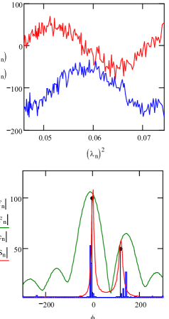
Refer to caption
Figure 1: RM-MUSIC successful result for two components with the complex amplitudes f1=100isubscript𝑓1100𝑖f_{1}=-100i, f1=50isubscript𝑓150𝑖f_{1}=50i, and Faraday depths ϕ0=0radm2subscriptitalic-ϕ00radsuperscriptm2\phi_{0}=0\,\mathrm{rad}\,\mathrm{m}^{-2}, ϕ1=122radm2subscriptitalic-ϕ1122radsuperscriptm2\phi_{1}=122\,\mathrm{rad}\,\mathrm{m}^{-2}, separated by ϕ1ϕ2δϕsimilar-to-or-equalssubscriptitalic-ϕ1subscriptitalic-ϕ2𝛿italic-ϕ\phi_{1}-\phi_{2}\simeq\delta\phi (|f|𝑓|f| component amplitudes, |F|𝐹|F| “dirty” FDF, |c|𝑐|c| RM-CLEAN components, S𝑆S RM-MUSIC spectrum).
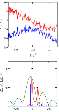
Refer to caption
Figure 2: RM-MUSIC successful result for two components with the complex amplitudes f1=100isubscript𝑓1100𝑖f_{1}=-100i, f1=50isubscript𝑓150𝑖f_{1}=50i, and Faraday depths ϕ0=0radm2subscriptitalic-ϕ00radsuperscriptm2\phi_{0}=0\,\mathrm{rad}\,\mathrm{m}^{-2}, ϕ1=61radm2subscriptitalic-ϕ161radsuperscriptm2\phi_{1}=61\,\mathrm{rad}\,\mathrm{m}^{-2}, separated by ϕ1ϕ20.5δϕsimilar-to-or-equalssubscriptitalic-ϕ1subscriptitalic-ϕ20.5𝛿italic-ϕ\phi_{1}-\phi_{2}\simeq 0.5\delta\phi (|f|𝑓|f| component amplitudes, |F|𝐹|F| “dirty” FDF, |c|𝑐|c| RM-CLEAN components, S𝑆S RM-MUSIC spectrum).
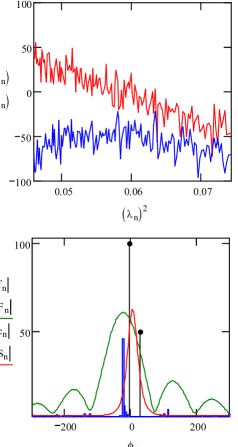
Refer to caption
Figure 3: RM-MUSIC result for two components with the complex amplitudes f1=100isubscript𝑓1100𝑖f_{1}=-100i, f1=50isubscript𝑓150𝑖f_{1}=50i, and Faraday depths ϕ0=0radm2subscriptitalic-ϕ00radsuperscriptm2\phi_{0}=0\,\mathrm{rad}\,\mathrm{m}^{-2}, ϕ1=30.5radm2subscriptitalic-ϕ130.5radsuperscriptm2\phi_{1}=30.5\,\mathrm{rad}\,\mathrm{m}^{-2}, separated by ϕ1ϕ20.25δϕsimilar-to-or-equalssubscriptitalic-ϕ1subscriptitalic-ϕ20.25𝛿italic-ϕ\phi_{1}-\phi_{2}\simeq 0.25\delta\phi (|f|𝑓|f| component amplitudes, |F|𝐹|F| “dirty” FDF, |c|𝑐|c| RM-CLEAN components, S𝑆S RM-MUSIC spectrum).
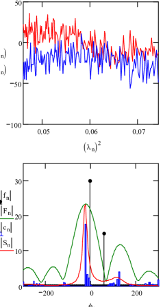
Refer to caption
Figure 4: RM-MUSIC result for low signal to noise is comparable to RM-CLEAN. Two components with f1=100isubscript𝑓1100𝑖f_{1}=-100i, f1=50isubscript𝑓150𝑖f_{1}=50i, Faraday depths ϕ0=0radm2subscriptitalic-ϕ00radsuperscriptm2\phi_{0}=0\,\mathrm{rad}\,\mathrm{m}^{-2}, ϕ1=61radm2subscriptitalic-ϕ161radsuperscriptm2\phi_{1}=61\,\mathrm{rad}\,\mathrm{m}^{-2}, separated by ϕ1ϕ20.5δϕsimilar-to-or-equalssubscriptitalic-ϕ1subscriptitalic-ϕ20.5𝛿italic-ϕ\phi_{1}-\phi_{2}\simeq 0.5\delta\phi (|f|𝑓|f| component amplitudes, |F|𝐹|F| “dirty” FDF, |c|𝑐|c| RM-CLEAN components, S𝑆S RM-MUSIC spectrum).

The RM-MUSIC method works very well when the components are separated above the resolution limit δϕ𝛿italic-ϕ\delta\phi. For example, in Figure 1 we have two components with the complex amplitudes f0=100isubscript𝑓0100𝑖f_{0}=-100i and f1=50isubscript𝑓150𝑖f_{1}=50i at λ2=λr2superscript𝜆2superscriptsubscript𝜆𝑟2\lambda^{2}=\lambda_{r}^{2}, and Faraday depths ϕ0=0radm2subscriptitalic-ϕ00radsuperscriptm2\phi_{0}=0\,\mathrm{rad}\,\mathrm{m}^{-2}, ϕ1=122radm2subscriptitalic-ϕ1122radsuperscriptm2\phi_{1}=122\,\mathrm{rad}\,\mathrm{m}^{-2}, separated by ϕ1ϕ0=δϕsubscriptitalic-ϕ1subscriptitalic-ϕ0𝛿italic-ϕ\phi_{1}-\phi_{0}=\delta\phi. For comparison we also give the “dirty” FDF and the RM-CLEAN components. In order to make the results comparable, we scaled S(ϕ)𝑆italic-ϕS(\phi) as S(ϕ)S(ϕ)|F|max|S|max1𝑆italic-ϕ𝑆italic-ϕsubscript𝐹𝑚𝑎𝑥superscriptsubscript𝑆𝑚𝑎𝑥1S(\phi)\leftarrow S(\phi)\left|F\right|_{max}\left|S\right|_{max}^{-1}, where |F|maxsubscript𝐹𝑚𝑎𝑥\left|F\right|_{max} and |S|maxsubscript𝑆𝑚𝑎𝑥\left|S\right|_{max} are the maximum amplitudes of the original spectra. This way, both S(ϕ)𝑆italic-ϕS(\phi) and |F(ϕ)|𝐹italic-ϕ\left|F(\phi)\right| are in the same range. One can see that the RM-MUSIC spectrum recovers almost exactly the Faraday depths of the two components ϕ~0=1.05radm2subscript~italic-ϕ01.05radsuperscriptm2\tilde{\phi}_{0}=1.05\,\mathrm{rad}\,\mathrm{m}^{-2}, ϕ~1=122.81radm2subscript~italic-ϕ1122.81radsuperscriptm2\tilde{\phi}_{1}=122.81\,\mathrm{rad}\,\mathrm{m}^{-2}, while both the “dirty” FDF and RM-CLEAN fail to recover the Faraday depth of the second component: ϕ~0=2.01radm2subscript~italic-ϕ02.01radsuperscriptm2\tilde{\phi}_{0}=2.01\,\mathrm{rad}\,\mathrm{m}^{-2}, ϕ~1=142.95radm2subscript~italic-ϕ1142.95radsuperscriptm2\tilde{\phi}_{1}=142.95\,\mathrm{rad}\,\mathrm{m}^{-2}. Moreover, once the depths are recovered, the real and imaginary parts of the RM components can be easily computed using a linear least squares fitting approach, resulting in an almost exact recovery: f~0=1.9599.74isubscript~𝑓01.9599.74𝑖\tilde{f}_{0}=-1.95-99.74i, f~1=0.05+50.02isubscript~𝑓10.0550.02𝑖\tilde{f}_{1}=0.05+50.02i.

In Figure 2 we show that the MUSIC super-resolution method can give good results even for separations below the the resolution in Faraday depth space δϕ𝛿italic-ϕ\delta\phi. Here, we have the same two components with Faraday depths ϕ0=0radm2subscriptitalic-ϕ00radsuperscriptm2\phi_{0}=0\,\mathrm{rad}\,\mathrm{m}^{-2}, ϕ1=61radm2subscriptitalic-ϕ161radsuperscriptm2\phi_{1}=61\,\mathrm{rad}\,\mathrm{m}^{-2}, separated by ϕ1ϕ0=0.5δϕsubscriptitalic-ϕ1subscriptitalic-ϕ00.5𝛿italic-ϕ\phi_{1}-\phi_{0}=0.5\delta\phi. One can see that both components are correctly separated by the RM-MUSIC spectrum ϕ~0=0radm2subscript~italic-ϕ00radsuperscriptm2\tilde{\phi}_{0}=0\,\mathrm{rad}\,\mathrm{m}^{-2}, f~0=0.84100.93isubscript~𝑓00.84100.93𝑖\tilde{f}_{0}=0.84-100.93i, ϕ~1=62.4radm2subscript~italic-ϕ162.4radsuperscriptm2\tilde{\phi}_{1}=62.4\,\mathrm{rad}\,\mathrm{m}^{-2}, f~1=0.76+51.49isubscript~𝑓10.7651.49𝑖\tilde{f}_{1}=-0.76+51.49i. and once again the “dirty” FDF and RM-CLEAN fail to recover the Faraday depths, showing two main components at: ϕ~0=6.4radm2subscript~italic-ϕ06.4radsuperscriptm2\tilde{\phi}_{0}=-6.4\,\mathrm{rad}\,\mathrm{m}^{-2}, and respectively ϕ~1=118.8radm2subscript~italic-ϕ1118.8radsuperscriptm2\tilde{\phi}_{1}=118.8\,\mathrm{rad}\,\mathrm{m}^{-2}. This is a typical example where the interference of pairs of RM components conspire to place the peak response of the FDF outside of the RM range between the two input RM components. In Figure 3 we consider the same two components separated by ϕ1ϕ00.25δϕsimilar-to-or-equalssubscriptitalic-ϕ1subscriptitalic-ϕ00.25𝛿italic-ϕ\phi_{1}-\phi_{0}\simeq 0.25\delta\phi, ϕ0=0radm2subscriptitalic-ϕ00radsuperscriptm2\phi_{0}=0\,\mathrm{rad}\,\mathrm{m}^{-2}, ϕ1=30.5radm2subscriptitalic-ϕ130.5radsuperscriptm2\phi_{1}=30.5\,\mathrm{rad}\,\mathrm{m}^{-2}. In this case the RM-MUSIC spectrum cannot separate the components anymore, however it correctly shows only one maximum, situated between the two input RM components, while RM-CLEAN suggests a single RM component outside the range of the input RMs.

From the above examples we see that RM-MUSIC performs better than RM-CLEAN for high to moderate S/N cases. However, in low S/N situations the performance of RM-MUSIC deteriorates. It is quite difficult to quantify the S/N ratio exactly and to find a limiting S/N value, and more future evaluations of the method are required for various wavelength ranges and noise levels per channel. For the considered experiment layout our numerical simulations have shown that if the amplitude of the strongest RM component is becoming smaller than |f0|50similar-to-or-equalssubscript𝑓050|f_{0}|\simeq 50, and for a noise per channel σ=N=12.247𝜎𝑁12.247\sigma=\sqrt{N}=12.247, RM-MUSIC begins to behave more like RM-CLEAN, and cannot separate correctly the input components. In Figure 4 we give such an example of two components with the complex amplitudes f0=30isubscript𝑓030𝑖f_{0}=-30i and f1=15isubscript𝑓115𝑖f_{1}=15i, Faraday depths ϕ0=0radm2subscriptitalic-ϕ00radsuperscriptm2\phi_{0}=0\,\mathrm{rad}\,\mathrm{m}^{-2} and ϕ1=61radm2subscriptitalic-ϕ161radsuperscriptm2\phi_{1}=61\,\mathrm{rad}\,\mathrm{m}^{-2}, separated by ϕ1ϕ00.5δϕsimilar-to-or-equalssubscriptitalic-ϕ1subscriptitalic-ϕ00.5𝛿italic-ϕ\phi_{1}-\phi_{0}\simeq 0.5\delta\phi. One can see that in this case, both RM-MUSIC and RM-CLEAN give similar results. We should also mention that the experiment layout used in simulations is very similar to the ASKAP’s POSSUM survey (Gaensler et al., 2010), where the expected final noise is 101010 μ𝜇\muJy/beam. This value suggests that for N=150𝑁150N=150 channels and a peak signal to noise threshold of 4similar-toabsent4\sim 4, RM-MUSIC should work as indicated for sources with polarized flux higher than 0.50.50.5 mJy/beam, which is rather bright but quite reasonable, since about 57%similar-toabsentpercent57\sim 57\% of the NVSS RM catalog sources fall into this category.

6 Conclusion

We have discussed a novel deconvolution method for RM synthesis applications, based on an extension of the MUSIC super-resolution algorithm. Numerical results show that for high to moderate S/N cases RM-MUSIC outperforms the standard RM-CLEAN approach, being able to recover Faraday depth values of closely spaced pairs of thin RM components, even in situations where the peak response of FDF is outside the range between the two input components. For low S/N cases, the RM-MUSIC and RM-CLEAN methods provide similar results. RM-MUSIC performs well for pairs of thin RM components, however it is not suitable when the input Faraday spectrum contains polarized emission at a continuous range of RM.

References

  • Andrecut et al. (2012) Andrecut, M., Stil, J. M., Taylor, A. R., 2012, AJ, 143, 33
  • Brentjens & de Bruyn (2005) Brentjens, M. & de Bruyn, A., 2005, A&A, 441, 1217
  • Cheney (2001) Cheney, M., 2001, Inverse Problems, 17, 591
  • Farnsworth et al. (2011) Farnsworth, D., Rudnick, L., Brown, S., 2011, AJ, 141, 191
  • Gaensler et al. (2010) Gaensler, B. M., Landecker, T. L., Taylor, A. R., 2010, BAAS, 42, 515
  • Frick et al. (2010) Frick, P., Sokoloff, D., Stepanov, R. & Beck, R., 2010, MNRAS, 401, L24
  • Heald et al. (2009) Heald, G., Braun, R., Edmonds, R., 2009, A&A 503, 409
  • Hogbom (1974) Hogbom, J. 1974, A&A Supp., 15, 417
  • Li et al. (2011) Li, F., Brown, S., Cornwell T. J. & de Hoog, F., 2011, A&A, 531, A126.