Asymptotically inspired moment-closure approximation for adaptive networks

Abstract

Adaptive social networks, in which nodes and network structure co-evolve, are often described using a mean-field system of equations for the density of node and link types. These equations constitute an open system due to dependence on higher order topological structures. We propose a new approach to moment closure based on the analytical description of the system in an asymptotic regime. We apply the proposed approach to two examples of adaptive networks: recruitment to a cause model and adaptive epidemic model. We show a good agreement between the improved mean-field prediction and simulations of the full network system.

I Introduction

In recent years we have seen much progress in the field of network dynamics and dynamics on networks Albert and Barabási (2002); Newman (2003); Boccaletti et al. (2006); Arenas et al. (2008). Strong interest in understanding phenomena such as disease spread on social networks, interaction online social media such as Facebook and Twitter, dynamics of neuronal networks, and many others have encouraged development of mathematical tools necessary to analyze the behavior of such systems B. Goncalves et al. (2011); Josic et al. (2009); T.J. Sejnowski and T. Poggio (2001); C. Moore and M. E. J. Newman (2000); Pastor-Satorras and Vespignani (2001).

Often the first step in analyzing such systems is to represent them as networks, where an individual unit, e.g., a person, a user account, a neuron, is represented by a node, and possibility of interaction between any two units is represented by a link between them. The dynamical processes on such networks are often characterized by their statistical properties via a mean-field approach Gross et al. (2006); Shaw and Schwartz (2008); Shkarayev et al. (2011); Jolad et al. (2011). Such mean-field equations consist of a hierarchy of equations, where the expected state of the nodes, due to interaction via the network, is coupled to the statistical description of links in the network. The dynamical evolution of the links in turn depends on the evolution of statistical description of node triples, which in turn depend on higher order structures, and so on. In other words, this mean-field description yields an infinite system of coupled equations, which usually must be truncated in order to be solvable. The truncated system is open and has to be closed by introducing additional information about the system.

The dynamics on network systems are often closed at the level of link equations, where the network information makes its first appearance Murrell et al. (2004). Perhaps the simplest closure approach is based on the assumption of homogeneous distribution of different node types in the system, and that the probability of finding a particular type of node in the neighborhood of a given node is independent of what else can be found in that node’s neighborhood. This closure was shown to produce excellent results for many different systems Keeling et al. (1997); Murrell et al. (2004); Rogers (2011); Taylor et al. (2012); Kiss et al. (2012); Kiss and Simon (2012). The heterogeneous mean-field approach, where conditioning on the total degree of nodes is introduced, may improve the accuracy of the approximation, although drastically increasing the number of equations in the description Vincent Marceau et al. (2010); Pastor-Satorras and Vespignani (2001). Often, additional information about the system, such as the expected clustering coefficient, may be used to improve the closure Taylor et al. (2012). In other cases, assumptions about the shape of degree distribution functions Kiss and Simon (2012), possibly guided by numerical simulations or physical observations Keeling et al. (1997); Keeling and Eames (2005), may lead to an improvement in closure. Equation-free approaches may also be used when closing the mean-field equations A. I. Reppas et al. (2012); Gross and Kevrekidis (2008).

All of the above closures often lead to a reasonable approximation of the system dynamics. However, they all suffer either from the lack of a priori knowledge of the validity of approximation or from having an excessive number of equations that must be analyzed. In this paper, we propose a new method that may lead to accurate closures and that also allows one to manage the expectation of the accuracy of the obtained closure. The proposed approach is based on simplification of the mean-field system of equations in some asymptotic regime. In the rest of the paper we demonstrate our approach by applying it to two adaptive network systems, i.e., networks where dynamical processes on the nodes affect the network structure, which in turn affects subsequent dynamics on the nodes Gross and Blasius (2008). In section II, we derive a closure for a system modeling recruitment to a cause Shkarayev et al. (2011). In section III we derive an improved closure for an adaptive epidemic model Gross et al. (2006).

Figure 1: 1 Schematic representation of node dynamics in the recruitment model. The nodes are born into the N-class at rate $\mu$; nodes die at rate $\theta$; the possible transitions between the classes are marked by the arrows and labeled with the corresponding rates ($\lambda_{1}$, $\lambda_{2}$, $\gamma$). 1 Link rewiring takes place at a rate $w$. 1 Example of a node triple.

II Adaptive Recruitment model

Our first example is a model for recruitment to a cause, introduced in Shkarayev et al. (2011). A society is modeled as a network in which some of its individuals represent a particular ideology and actively recruit new members. These nodes are referred to as the recruiting nodes, or R-nodes. The rest of the people in the society are either susceptible to recruitment or non-susceptible, referred to as S- and N-nodes respectively. The N-nodes may spontaneously change their state and become S-nodes, and vice versa, at rates $\lambda_{1}$ and $\lambda_{2}$, respectively. The R-nodes recruit S-nodes at a recruitment rate $\gamma$ per contact with S-node. A schematic representation of these transitions appears in Fig. 1. The R-nodes can improve their recruiting capability by abandoning their connections to N-nodes in favor of S-nodes, as shown in Fig 1. This rewiring process takes place at a rate $w$ per contact between R- and N-nodes. The system is open in the sense that nodes die at rate $\theta$ per node, and new nodes enter the system at rate $\mu$. The newborn nodes are born as N-nodes, and attach themselves with links to $\sigma$ randomly chosen nodes.

In order to describe the evolution of this system, we begin with developing a heterogeneous mean-field description Vincent Marceau et al. (2010). We characterize the time evolution of $\rho_{\alpha;{\bf k}}$, the expected number of nodes of type $\alpha$ with $k_{1}$, $k_{2}$, and $k_{3}$ neighbors of type N, S, and R, respectively, in their neighborhoods, where ${\bf k}=(k_{1},k_{2},k_{3})$:

$$\begin{split}&\partial_{t}\rho_{N;{\bf k}}=\\ &\lambda_{2}\rho_{S;{\bf k}}-\lambda_{1}\rho_{N;{\bf k}}-\theta\rho_{N;{\bf k}}+\mu\delta_{k_{1}+k_{2}+k_{3},\sigma}\\ &+\sum_{i}\left[\Omega_{N;{\bf k}-r_{i}}(r_{i})\rho_{N;{\bf k}-r_{i}}-\Omega_{N;{\bf k}}(r_{i})\rho_{N;{\bf k}}\right],\end{split}$$ (1a)

$$\begin{split}&\partial_{t}\rho_{S;{\bf k}}=\\ &-\lambda_{2}\rho_{S;{\bf k}}-\gamma k_{3}\rho_{S;{\bf k}}+\lambda_{1}\rho_{N;{\bf k}}-\theta\rho_{S;{\bf k}}+\\ &+\sum_{i}\left[\Omega_{S;{\bf k}-r_{i}}(r_{i})\rho_{S;{\bf k-r_{i}}}-\Omega_{S;{\bf k}}(r_{i})\rho_{S;{\bf k}}\right].\end{split}$$ (1b)

$$\begin{split}&\partial_{t}\rho_{R;{\bf k}}=\gamma k_{3}\rho_{S;{\bf k}}-\theta\rho_{R;{\bf k}}+\\ &+\sum_{i}\left[\Omega_{S;{\bf k}-r_{i}}(r_{i})\rho_{S;{\bf k-r_{i}}}-\Omega_{S;{\bf k}}(r_{i})\rho_{S;{\bf k}}\right].\end{split}$$ (1c)

The allowed transitions and the corresponding rates shown in the Table 1. In the recruiting transition rates listed in the table, function $P$ (function $Q$) corresponds to the expected number of node chains that originate at a given N-node (S-node) with a neighborhood specified by ${\bf k}$ that is connected to an S-node, which is turn is connected to an R-node. The terms $N_{\text{X}_{1}\ldots\text{X}_{n}}$ correspond to the expected number of node chains in the system, where a node chain constitutes a set of nodes, connected as follows: a node of type $X_{1}$ is connected to the node of type $X_{2}$, which in turn is connected to node of type $X_{3}$ etc. For example, $N_{S}$ is the expected number of S-nodes in the network, while $N_{\text{RS}}$ is the expected number of links with S- and R-nodes at its ends. In our definition of node chains we require the $i$th and $i+1$st nodes to be different; however, $i$th and $i+2$nd nodes can in fact be the same node. In the example of a network presented in Fig. 1 there are 4 RSR triples, corresponding to the following node combinations: 1-2-1, 1-2-3, 3-2-1, 3-2-3. Note that the order in which nodes appear matters, which, for example, means that $N_{\text{SS}}$ corresponds to the twice the expected number of undirected links between two susceptible nodes.

Table 1: Transitions and nonzero transition rates in

Eq. (1) transition rate $r_{1}=(-1,1,0)$ $\Omega_{N;{\bf k}}(r_{1})=\Omega_{S;{\bf k}}(r_{1})=\Omega_{R;{\bf k}}(r_{1})=\lambda_{1}k_{1}$ $r_{2}=(1,-1,0)$ $\Omega_{N;{\bf k}}(r_{2})=\Omega_{S;{\bf k}}(r_{2})=\Omega_{R;{\bf k}}(r_{2})=\lambda_{2}k_{2}$ $r_{3}=(-1,0,0)$ $\Omega_{N;{\bf k}}(r_{3})=\Omega_{S;{\bf k}}(r_{3})=\Omega_{R;{\bf k}}(r_{3})=\theta k_{1}$ $r_{4}=(0,-1,0)$ $\Omega_{N;{\bf k}}(r_{4})=\Omega_{S;{\bf k}}(r_{4})=\Omega_{R;{\bf k}}(r_{4})=\theta k_{2}$ $r_{5}=(0,0,-1)$ $\Omega_{N;{\bf k}}(r_{5})=\Omega_{S;{\bf k}}(r_{5})=\Omega_{R;{\bf k}}(r_{5})=\theta k_{3}$ $r_{6}=(1,0,0)$ $\Omega_{N;{\bf k}}(r_{6})=\Omega_{S;{\bf k}}(r_{6})=\Omega_{R;{\bf k}}(r_{6})=$ $=\sigma\mu/(N_{N}+N_{S}+N_{R})$ $r_{7}=(0,-1,1)$ $\Omega_{N;{\bf k}}(r_{7})=\gamma P({\bf k})$, $\Omega_{S;{\bf k}}(r_{7})=\gamma Q({\bf k})$ $r_{8}=(0,0,-1)$ $\Omega_{N;{\bf k}}(r_{8})=wk_{3}$ $r_{9}=(0,0,1)$ $\Omega_{S;{\bf k}}(r_{9})=wN_{\text{RN}}/N_{S}$ $r_{10}=(-1,1,0)$ $\Omega_{R;{\bf k}}(r_{10})=wN_{\text{RN}}/N_{S}$

The heterogeneous mean-field equations are high dimensional and, therefore, are extremely difficult to analyze. A common way to analyze the dynamics of social networks is via lower dimensional mean-field equations. These can be generated by multiplying the heterogeneous mean-field equations by $k_{1}^{i_{1}}k_{2}^{i_{2}}k_{3}^{i_{3}}$ for some non-negative integer values of $i_{j}$, and summing over ${\bf k}$. Thus, the equations describing node dynamics are obtained by taking $i_{1}+i_{2}+i_{3}=0$, as given in Eqs. (25a)-(25c) of Appendix B, while the description of the link dynamics is obtained by taking $i_{1}+i_{2}+i_{3}=1$, as given in Eqs. (25d)-(25i).

The hierarchy of equations generated in this manner must be truncated in order to obtain a finite dimensional description of the system. Such truncation leaves the system open and in need of closure. For example, the system of node and link equations in (25) contains the terms $N_{\text{NSR}}$, $N_{\text{SSR}}$ and $N_{\text{RSR}}$, which are higher order structures. The usual approach to closure comes from the assumption of homogeneous distribution of the R-nodes in the neighborhood of susceptible nodes, which leads to the following closure equations:

$$\frac{N_{\text{XSR}}}{N_{S}}=\frac{N_{\text{XS}}}{N_{S}}\frac{N_{\text{RS}}}{N_{S}},$$ (2a)

$$\frac{N_{\text{RSR}}}{N_{S}}=\left(\frac{N_{\text{RS}}}{N_{S}}\right)^{2}+\frac{N_{\text{RS}}}{N_{S}},$$ (2b)

where we also assumed that the degree distribution of susceptible nodes is Poisson. The details of these closures are presented in the Appendix A. These closures are ad hoc and may fail to capture the system behavior accurately if, for example, correlations are present. Here we develop an approach that derives the closure based on the system behavior in some asymptotic regime. In particular, we derive the equations that describe the evolution of node triples, take a steady-state relation and consider it in the asymptotic regime, where we are able to close the equations. Finally, we numerically explore the performance of the derived closures in parameter regimes outside of the asymptotic limit and outside of the steady-state.

II.1 Closing of NSR and SSR terms

We develop a closure of the $N_{\text{NSR}}$ and $N_{\text{SSR}}$ terms by considering the evolution of the expected number of node triples in the limit of $\gamma,\theta,\mu/(N_{N}+N_{S}+N_{R})\ll w,\lambda_{1},\lambda_{2}$. We consider the following expression:

$$\begin{split}&\sum_{{\bf k}}\left(\frac{N_{\text{RS}}}{N_{S}}\frac{\partial_{t}\rho_{S;{\bf k}}}{N_{N}}+\frac{N_{\text{RN}}}{N_{N}}\frac{\partial_{t}\rho_{N;{\bf k}}}{N_{N}}\right)\left(k_{1}k_{3}+k_{2}k_{3}\right).\end{split}$$ (3)

This relation is evaluated at the steady state and using Eq. (26a) and (26b). After some algebraic manipulations described in Appendix C, the above relation leads to

$$\begin{split}&\frac{N_{\text{NSR}}}{N_{S}}+\frac{N_{\text{SSR}}}{N_{S}}=\frac{N_{\text{SN}}}{N_{S}}\frac{N_{\text{RS}}}{N_{S}}+\frac{N_{\text{SS}}}{N_{S}}\frac{N_{\text{RS}}}{N_{S}}\end{split}$$ (4)

a result that is consistent with but does not imply the closure in Eqs. (2a) for $X=N$ and $S$.

We compare the asymptotically derived result of Eq. (4) and the ad hoc closure for the $N_{\text{SSR}}$ term in Eq. (2a) with the corresponding values measured in the Monte Carlo simulations. Figure 2 presents the relative error of the two closures

$$\Delta=\left|1-\frac{\text{approximation}}{\text{exact value}}\right|$$ (5)

where simulation measurements are used as the exact value. We can see in Fig. 2(a) that the expected number of NSR and SSR triples per susceptible node, $N_{\text{NSR}}/N_{S}+N_{\text{SSR}}/N_{S}$, is well approximated (error on the order of about 1% or less) by the closure of Eq. (4) in the large $\lambda_{1}$ and $\lambda_{2}$ limit, further improving as $w$ is increased. According to Fig. 2(c), the closure of $N_{\text{NSR}}/N_{S}+N_{\text{SSR}}/N_{S}$ continues to hold even in the parameter regime outside of the considered limit. As for the individual closures, Fig. 2(b) shows that the closure of $N_{\text{SSR}}/N_{S}$ holds as well in the large $\lambda_{1}$ and $\lambda_{2}$ regime. However, as we can see in Fig. 2(d), the closure fails for small $\lambda_{1}$ and $\lambda_{2}$, especially as $\gamma$ becomes dominant. Since the closure of $N_{\text{SSR}}/N_{S}+N_{\text{NSR}}/N_{S}$ is derived in the asymptotic regime, we expect it to be accurate at least in that limit, while $N_{\text{SSR}}/N_{S}$ closure is still ad hoc, and, therefore, deviation from simulations is not unexpected.

(a) $N_{\text{SSR}}+N_{\text{NSR}}$ $\lambda_{1}=10^{1},\lambda_{2}=10^{2}$

(b) $N_{\text{SSR}}$   $\lambda_{1}=10^{1},\lambda_{2}=10^{2}$

(c) $N_{\text{SSR}}+N_{\text{NSR}}$ $\lambda_{1}=10^{-1},\lambda_{2}=10^{0}$

(d) $N_{\text{SSR}}$ $\lambda_{1}=10^{-1},\lambda_{2}=10^{0}$

Figure 2: Relative errors in $N_{\text{NSR}}+N_{\text{SSR}}$ closure (Eq. (4)) (panels a,c) and $N_{\text{SSR}}$ closure (Eq. (2a)) (panels b,d) at steady state, as a function of $\gamma$ for $w=10^{0}$ (circle, green online), $w=10^{1}$ (triangle, red online), $w=10^{2}$ (cross, black online). The simulations are performed following the continuous time algorithm introduced in Gillespie (1976). The other parameters are $\theta=1$, $\sigma=10$, $\mu=10^{5}$.

II.2 Closure of RSR term

In order to develop a closure for the $N_{\text{RSR}}$ term, we consider the expression

$$\begin{split}&\sum_{{\bf k}}k_{3}^{2}\partial_{t}\rho_{S;{\bf k}},\end{split}$$ (6)

which leads to the equation describing the evolution of the expected number of RSR triples:

$$\begin{split}&\partial_{t}N_{\text{RSR}}=-\lambda_{2}N_{\text{RSR}}-\gamma\sum_{{\bf k}}k_{3}^{3}\rho_{S;{\bf k}}({\bf k})+\\ &\lambda_{1}N_{\text{RNR}}-\theta N_{\text{RSR}}+\gamma(2N_{\text{RSSR}}+N_{\text{SSR}})+\\ &w\frac{N_{\text{RN}}}{N_{S}}(2N_{\text{RS}}+N_{S})+\theta(-2N_{\text{RSR}}+N_{\text{RS}}).\end{split}$$ (7)

Analyzing the steady state of this equation in the limit where $\gamma,\theta,\mu/(N_{N}+N_{S}+N_{R})\ll w,\lambda_{1},\lambda_{2}$, and utilizing the relations in Eqs. (26a) and (26b), we are able to solve this equation and obtain the following relation:

$$\frac{N_{\text{RSR}}}{N_{S}}=\left(\frac{N_{\text{RS}}}{N_{S}}-\frac{N_{\text{RN}}}{N_{N}}\right)\left(2\frac{N_{\text{RS}}}{N_{S}}+1\right)+\frac{N_{\text{RNR}}}{N_{N}}.$$ (8)

Note that, unlike the ad hoc closure of Eq. (2b), this result should at least be accurate in the considered limit, and, therefore should be more reliable.

In order to close the $N_{\text{RNR}}/N_{N}$ term in Eq. (8) we analyze the limiting behavior of the following expression:

$$\begin{split}&\sum_{{\bf k}}k_{3}^{2}[\partial_{t}\rho_{S;{\bf k}}+\partial_{t}\rho_{N;{\bf k}}],\end{split}$$ (9)

which in steady state reduces to:

$$\frac{N_{\text{RNR}}}{N_{N}}=\frac{N_{\text{RN}}}{N_{N}}+\frac{N_{\text{RN}}}{N_{N}}\frac{N_{\text{RS}}}{N_{S}}$$ (10)

Upon substituting the result of Eq. (10) into Eq. (8) we obtain the following closure of the $N_{\text{RSR}}/N_{S}$ term:

$$\frac{N_{\text{RSR}}}{N_{S}}=2\left(\frac{N_{\text{RS}}}{N_{S}}\right)^{2}+\frac{N_{\text{RS}}}{N_{S}}-\frac{N_{\text{RS}}}{N_{S}}\frac{N_{\text{RN}}}{N_{N}}.$$ (11)

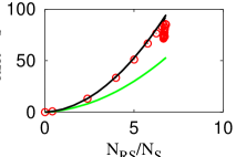
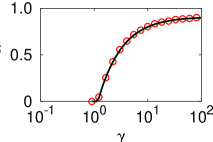
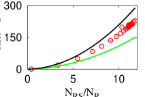
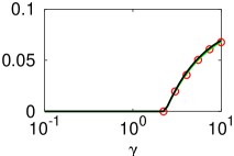
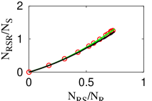
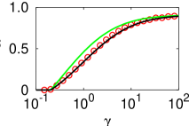
In Fig. 3, we compare the performance of the new closure of $N_{\text{RSR}}$ in Eq. (11) to the ad hoc, homogeneity based closure of Eq. (2b). We consider the numerical solution of the mean-field equations, found in Appendix B, closed according to the two methods, and compare those to the steady-state size of the recruiting class measured in the direct network simulations. In both cases, the $N_{\text{NSR}}$ and $N_{\text{SSR}}$ terms are closed according to the homogeneity assumption in Eq. (2a). Thus, in Fig. 3(a) we see that in the considered limit, i.e., when $\lambda_{1},\lambda_{2}$ and $w$ are large, the mean-field closed using our approach is in much better agreement with the simulations than the ad hoc assumption of Eq. (2b). The reason for the superior performance lies in the better approximation of the $N_{\text{RSR}}/N_{S}$ term, shown in Fig. 3(b). Here $N_{\text{RSR}}/N_{S}$ and $N_{\text{RS}}/N_{S}$ are parametrized by $\gamma$, with larger values of $N_{\text{RS}}/N_{S}$ corresponding to the larger values of $\gamma$. Notice that the performance of the closure is reduced at the larger values of $\gamma$, as the system moves outside of the considered limit.

(a) $\lambda_{1}=10^{1},\lambda_{2}=10^{2}$ $w=10^{2}$

(b) $\lambda_{1}=10^{1},\lambda_{2}=10^{2}$ $w=10^{2}$

(c) $\lambda_{1}=10^{1},\lambda_{2}=10^{2}$ $w=10^{-1}$

(d) $\lambda_{1}=10^{1},\lambda_{2}=10^{2}$ $w=10^{-1}$

(e) $\lambda_{1}=10^{-1},\lambda_{2}=10^{0}$ $w=10^{2}$

(f) $\lambda_{1}=10^{-1},\lambda_{2}=10^{0}$ $w=10^{2}$

(g) $\lambda_{1}=10^{-1},\lambda_{2}=10^{0}$ $w=10^{-1}$

(h) $\lambda_{1}=10^{-1},\lambda_{2}=10^{0}$ $w=10^{-1}$

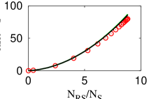
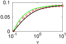
Figure 3: Recruitment level, $N_{R}$, and expected number of RSR triples per S-node, $N_{\text{RSR}}/N_{S}$, as a function of recruitment rate $\gamma$, for several sets of parameters $\lambda_{1}$, $\lambda_{2}$ and $w$. Simulation results are shown by circles (red online). In 3(a), 3(c), 3(e) and 3(g), the curves correspond to solution of mean-field equations, while in 3(b), 3(d), 3(f) and 3(h) the curves correspond to the approximation of $N_{\text{RSR}}/N_{S}$ using two different closures. Dark curves (black online) correspond to closure in Eq. (11), while light curves (green online) correspond to closure in Eq. (2b). The other parameters are same as in Fig. 2. Note that in Fig. 3(c), 3(d), 3(g), and 3(h) the curves corresponding to the two analytic solutions lie on top of each other.

The appeal of this approach is evident when we test it outside of the derivation limit. In Figs. 3(c) and 3(d) we see that, when we reduce $w$, the mean-field recruited fraction and the RSR closure continue to be in a good agreement with the simulations. We also note that in this limit the new closure approaches the homogeneity closure. We note that when the rewiring is slow relative to transitions between N and S, the expected number of R neighbors should be similar for the two node types. This would make the last term in Eq. (11) approach $(N_{\text{RS}}/N_{S})^{2}$, explaining why the two closures are close. In Fig. 3(e), as $\lambda_{1}$ and $\lambda_{2}$ are reduced, the new mean-field solution appears to be less consistent with the simulations, which is also reflected in the closure in Fig. 3(f). Finally, in Fig. 3(g) all of the parameters are about the same order, and yet the asymptotically derived closure and the corresponding mean-field are very much consistent with the simulations.

Thus far we have shown that our method has produced a closure that is a good match for the simulated system in steady-state, and is either superior to or as good as the ad hoc homogeneity closure. We further test the performance of our closure by using it outside of steady-state. Figures 4 and 4 show that our closure continues to be consistent with the simulations even during the transient period. This suggests that the time derivative of $N_{\text{RSR}}$ in Eq. (7) can be neglected in the considered limit.

Figure 4: Figure 4 contains measurement and approximation of $N_{R}$. The circles (red online): simulation results, the light curve (green online): mean-field with homogeneous closure, the dark curve (black online): mean-field with asymptotically developed closure from Eq. (11). Figure 9 shows the time evolution of the number of RSR triples per S-node (circles, red online), the approximate value obtained from the relation in Eq. (2b) (light curve, green online) and from Eq. (11) (dark curve, black online). The simulations are performed with $w=10^{2}$, $\lambda_{1}=10^{1}$, $\lambda_{2}=10^{2}$ and $\gamma=3.0$. The system evolves from a realization of Erdös-Rényi network, with mean degree $10$ and $10^{5}$ nodes, 85% of which are N-nodes, 5% S-nodes and 10% R-nodes. The results are averaged over 10 dynamical realizations.

III Adaptive Epidemic model

The other example that we consider is a model for epidemic spread on an adaptive social network Gross et al. (2006). Here the disease spread is described using the susceptible-infected-susceptible model, where each individual in the society is in one of the two states: sick or infected, and healthy but susceptible to infection. In the framework of networks, we refer to these as I- and S-nodes respectively. The infected individuals become susceptible at recovery rate $r$. The disease can spread at a rate $p$ from infected individuals to susceptible ones via a contact between them, where the existence of the contact is defined by the network structure. The adaptation mechanism allows susceptible individuals to change their local connectivity to avoid contact with infected individuals. Thus, the susceptibles rewire their contacts away from infecteds at rate $w$, connecting instead to a randomly chosen susceptible. The node and link dynamical rules are summarized in the Fig. 5 and 5 respectively.

Figure 5: Schematic representation of 5 node dynamical rules and 5 link dynamical rules in the adaptive epidemic model.

The evolution of the ensemble average of such a system is described by the set of heterogeneous mean-field equations:

$$\begin{split}&\partial_{t}{\rho}_{S;{{\bf k}}}=r{\rho}_{I;{{\bf k}}}-pk_{2}{\rho}_{S;{{\bf k}}}+\\ &+\sum_{i}\left[{\Omega}_{S;{{\bf k}}-r_{i}}(r_{i}){\rho}_{S;{{\bf k}}-r_{i}}-{\Omega}_{S;{{\bf k}}}(r_{i}){\rho}_{S;{{\bf k}}}\right],\end{split}$$ (12a)

$$\begin{split}&\partial_{t}{\rho}_{I;{{\bf k}}}=-r{\rho}_{I;{{\bf k}}}+pk_{2}{\rho}_{S;{{\bf k}}}+\\ &+\sum_{i}\left[{\Omega}_{I;{{\bf k}}-r_{i}}(r_{i}){\rho}_{I;{{\bf k}}-r_{i}}-{\Omega}_{I;{{\bf k}}}(r_{i}){\rho}_{I;{{\bf k}}}\right],\end{split}$$ (12b)

where the value of ${\rho}_{S;{{\bf k}}}$ (value of ${\rho}_{I;{{\bf k}}}$) corresponds to the number of S-nodes (I-nodes) with $k_{1}$ of S-nodes and $k_{2}$ of I-nodes in their neighborhoods, with ${{\bf k}}\equiv(k_{1},k_{2})$. The function $K$ (function $M$) corresponds to the expected number of node chains that originate at an S-node (I-node) with a neighborhood specified by ${\bf k}$, which connects to an S-node, which in turn connects to an I-node. The functions $N_{\text{X}_{1}\ldots\text{X}_{n}}$ are defined in the same way as in Section II.

Table 2: Transitions and nonzero transition rates in Eq. (12).

transitions	non-zero rates
$r_{1}=(1,-1)$	${\Omega}_{I;{{\bf k}}}(r_{1})={\Omega}_{S;{{\bf k}}}(r_{1})=rk_{2}$
$r_{2}=(-1,1)$	${\Omega}_{S;{{\bf k}}}(r_{2})=pK({{\bf k}})$, ${\Omega}_{I;{{\bf k}}}(r_{2})=pM({{\bf k}})$
$r_{3}=(1,-1)$	${\Omega}_{S;{{\bf k}}}(r_{3})=wk_{2}$
$r_{4}=(1,0)$	${\Omega}_{S;{{\bf k}}}(r_{4})=wN_{\text{IS}}/N_{S}$
$r_{5}=(-1,0)$	${\Omega}_{I;{{\bf k}}}(r_{5})=wk_{1}$

The mean-field equations are generated by multiplying the heterogeneous mean-field equations by $k_{1}^{i_{1}}k_{2}^{i_{2}}$ and summing over ${\bf k}$, where $i_{1}$ and $i_{2}$ are nonnegative integers. Thus, two node equations are generated for $i_{1}+i_{2}=0$, and three distinct link equations are generated for $i_{1}+i_{2}=1$. These equations, presented in the appendix as Eqs. (33a)-(33e), are open due to dependence on terms describing the expected number of ISI triples, $N_{\text{ISI}}$, and SSI triples, $N_{\text{SSI}}$. In order to close this system of equations, additional information is required. Once again, the usual approach Keeling et al. (1997) is to make an assumption that infected nodes are homogeneously distributed in the neighborhood of S-nodes, an assumption that leads to the following closure:

$$\frac{N_{\text{SSI}}}{N_{S}}=\frac{N_{\text{SS}}}{N_{S}}\frac{N_{\text{IS}}}{N_{S}},$$ (13a)

$$\frac{N_{\text{ISI}}}{N_{S}}=\left(\frac{N_{\text{IS}}}{N_{S}}\right)^{2}+\frac{N_{\text{IS}}}{N_{S}},$$ (13b)

where we make an additional assumption that the total degree distribution of susceptible nodes is Poisson. More details can be found in Appendix A.

Figure 6: Schematic representation of four-node chains I-S-S-I. The term $N_{\text{ISSI}}$ corresponds to the expected number of such chains.

We derive a new closure of the ISI term by first considering the evolution of the number of ISI triples. Multiplying equation (12a) by $k_{2}^{2}$ and summing over ${\bf k}$ at steady state,

$$\begin{split}\sum_{{\bf k}}k_{2}^{2}\partial_{t}{\rho}_{S;{{\bf k}}}=0,\end{split}$$ (14)

we obtain the following equation:

$$\begin{split}&0=rN_{\text{III}}-p\sum_{{\bf k}}[k_{2}^{3}{\rho}_{S;{{\bf k}}}]+\\ &+(r+w)[-2N_{\text{ISI}}+N_{\text{IS}}]+p[2N_{\text{ISSI}}+N_{\text{SSI}}],\end{split}$$ (15)

where the four-point term ISSI corresponds to the total number of node configurations shown in Fig. 6. Using the steady-state relations in Eqs. (35a) and (35b), we arrive at

$$\begin{split}&2(r+w)N_{S}\left(\frac{N_{\text{ISI}}}{N_{S}}-\frac{N_{\text{IS}}}{N_{S}}-\frac{N_{\text{IS}}}{N_{S}}\frac{N_{\text{ISSI}}}{N_{\text{SSI}}}\right)=\\ &=rN_{I}\left(\frac{N_{\text{III}}}{N_{I}}-\frac{N_{\text{II}}}{N_{I}}\frac{\sum_{{\bf k}}[k_{2}^{3}{\rho}_{S;{{\bf k}}}]}{\sum_{{\bf k}}[k_{2}^{2}{\rho}_{S;{{\bf k}}}]}\right).\end{split}$$ (16)

The left hand side of the equation corresponds to the flux of the expected number of ISI triples due to the changes in the neighborhood of the susceptible nodes, while the right hand side corresponds to the flux due to the infection and recovery of the susceptible node in the ISI triple. In the limit of large infection rate and weak rewiring, the amount of time any node spends in the susceptible state approaches zero. Therefore, it is reasonable to assume that the flux of triples due to the changes in the neighborhood of the susceptible node will approach zero as well. This leads us to conclude that the two sides of Eq. 16 must vanish, leaving us with the following relation:

$$\frac{N_{\text{ISI}}}{N_{S}}=\frac{N_{\text{IS}}}{N_{S}}+\frac{N_{\text{IS}}}{N_{S}}\frac{N_{\text{ISSI}}}{N_{\text{SSI}}}$$ (17)

Finally, we note that the term $N_{\text{ISSI}}/N_{\text{SSI}}$ corresponds to the expected number of I-nodes, node 1 in Fig. 6, attached to the chain of nodes numbered 2, 3 and 4 in that figure. This relation is well approximated by the homogeneity assumption, that the information about the neighborhood of the 3rd node in Fig. 6 has no effect on the information about the neighborhood of the 2nd node. In other words, the following moment closure is considered:

$$\frac{N_{\text{ISSI}}}{N_{\text{SSI}}}=\frac{N_{\text{SSI}}}{N_{\text{SS}}}.$$ (18)

In other words, we make a homogeneity assumption about the neighborhood of a neighbor, and we expect this assumption to be more accurate than the same assumption about a given node’s neighborhood, i.e., the closures in Eqs. (13a) and (13b).

(a)  $p/r=10^{-1/2}$

(b)  $p/r=10^{-1/2}$

(c)  $p/r=10^{0}$

(d)  $p/r=10^{0}$

(e)  $p/r=10^{1}$

(f)  $p/r=10^{1}$

Figure 7: Number of ISI triples per S-node as a function of rewiring rate, for several infection rates: simulations compared to the moment closures of Eq. (13b) and Eq. (19). Figures 7(a), 7(c), and 7(e) show $N_{\text{ISI}}/N_{S}$ measured in simulation (circles, red online), approximated using homogeneity closure of Eq. (13b) (light curve, green online), and approximated using the result of asymptotic analysis in Eq. (19) (dark curve, black online). The closures are evaluated using node and link quantities measured in the simulations. Light curves (green online) in figures 7(b), 7(d), and 7(f) show the relative error, Eq. (5), of the homogeneity approximation, while dark curves (black online) show the relative error due to the newly derived approximation. Cusps in the relative error curves correspond to the $N_{\text{ISI}}/N_{S}$ homogeneity closure curve crossing through the curve measured in simulations. Simulations are performed on a network with $10^{5}$ nodes and $5\times 10^{5}$ links following algorithm in Gillespie (1976).

(a) $w/r=10^{-1}$

(b) $w/r=10^{-1}$

(c) $w/r=10^{0}$

(d) $w/r=10^{0}$

(e) $w/r=10^{1}$

(f) $w/r=10^{1}$

Figure 8: Number of ISI triples per S-node as a function of infection rate, for several rewiring rates: simulations compared to two approximations. The curves and circles are defined as in Fig. 7, with the same network size and number of links.

Thus, we have derived a new closure of $N_{\text{ISI}}$:

$$\frac{N_{\text{ISI}}}{N_{S}}=\frac{N_{\text{IS}}}{N_{S}}+\frac{N_{\text{IS}}}{N_{S}}\frac{N_{\text{SSI}}}{N_{\text{SS}}},$$ (19)

which relies on our ability to close the $N_{\text{SSI}}$ term, and this brings us one step closer to finding an accurate closure of the mean-field description of the adaptive epidemic model (33). Curiously, the homogeneity closure of $N_{\text{SSI}}$ in Eq. (13a), together with Eq. (19), leads to the homogeneity closure in Eq. (13b). Thus, as is suggested by Figs. 7 and 8, where the measured values of $N_{\text{SSI}}$ are used, improving the closure of $N_{\text{SSI}}$ beyond the homogeneity assumption leads to improvement of the $N_{\text{ISI}}$ closure. In fact, Figs 7(b), 7(d), 7(f) as well as 8(b), 8(d), 8(f) show the relative deviation of the closure relations from the approximated quantity and suggest that the new approximation in Eq. (19) is superior to the relation in Eq. (13b). Note that the only time the homogeneity closure appears to perform better is when it intersects the measured value of $N_{\text{ISI}}/N_{S}$, and, therefore, its superiority over the performance of the new closure is rather coincidental. Further consideration of the results in Fig. 7 shows that, as we move away from the derivation regime of slow rewiring rates, the performance of the new closure diminishes, though it is still superior to the old approximation. Predictably, as shown in Fig. 8, the performance of the new approximation improves for the larger values of infection rate, and outperforming the original closure even near the epidemic threshold.

Finally, we test our new closure outside of the steady-state. Thus, Fig. 9 compares the performance of the newly derived approximation to that of the homogeneity approximation. We can see that, unlike the homogeneity closure, the new closure follows the measured values of $N_{\text{ISI}}/N_{S}$ very accurately. Furthermore, as shown in Fig. 9, the closure of Eq. (19) performs better as the solution approaches the steady-state.

Figure 9: Time evolution of ISI closure. Fig. 9 shows the time evolution of the number of ISI triples per S-node (circles, red online) and the approximate value as obtained from the relation in Eq. (13b) (light curve, green online) and from Eq. (19) (dark curve, black online). Fig. 9 shows the relative error due to the two approximations. The simulations are performed for $w=10^{-1}$, $p=10^{0}$, $r=1$, $10^{5}$ nodes and $5\times 10^{5}$ links. The initial network is a realization of an Erdös-Rényi random network; the state of each node is randomly assigned, with 90% I-nodes and 10% S-nodes. We take the average over 100 dynamical realizations.

IV Discussion

We presented an approach for closing a mean-field description of dynamical network systems. In our approach we proposed exploiting the possible simplification of the heterogeneous mean-field description of the system in some asymptotic regime. We applied this approach to two examples of adaptive networks: recruitment to a cause model and a model of epidemic spread on an adaptive network. Using the two examples, we successfully developed closures that perform as well as or better than the usual closures, which are based on the assumptions of homogeneous distribution of nodes throughout the network.

The closure we developed for the recruitment model showed significant improvement of the mean-field description over the one where all of the high order terms were approximated using the homogeneity closure. Not only do we see an improvement in the predicted levels of the recruited population; we also see greater consistency between the moment closure approximation and direct measurements of the closed terms. Thus, out of the three node-triple terms that we approximated, one showed significant improvement over the homogeneity based closure, and the sum of the remaining two triples proved to be consistent with the homogeneity closure.

In case of the epidemic model, the closure developed with the asymptotic approach also showed improvement over the ad hoc, homogeneity based closure. The result of utilizing our approach was an improved moment closure approximation for one of the terms, contingent on improvements of a closure for the other term, as confirmed by the numerical simulations of the adaptive system.

It is important to note that the closures that we derived in some asymptotic regimes proved to be more accurate than the homogeneity closures even outside of the derivation limit. For example, even though in both cases the closures were derived at steady-state, they showed excellent results outside of the asymptotic parameter regime where the derivation took place, as well as during the transient state of the dynamical process. The additional benefit of using this approach is that it allows us to expect good performance of the closure at least in the limit where the derivation took place, more than can be said about any ad hoc moment closure approximation. However, the more rigorous statements about the accuracy of this approach as well as the applicability of this approach to a more general class of network problems are left to the future investigations.

Appendix A Homogeneity Closure

The homogeneity closure is based on the assumption that the probability of finding an R-node at the end of a link that stems from an S-node is independent of what else is in the neighborhood of that S-node and is given by $q=N_{\text{RS}}/(N_{\text{RS}}+N_{\text{SS}}+N_{\text{SN}})$. In other words, the probability for the S-node to have $r$ of R-nodes in its neighborhood is assumed to be independent of the number of X-nodes in the neighborhood where X represents the other node types:

$$P_{S;n_{R}|n_{X}}(r|x)=P_{S;n_{R}}(r)$$ (20)

where $P_{S;n_{R}|n_{X}}(r|x)$ is the probability $r$ of the R-nodes are in the neighborhood of the S-node conditioned on the presence of $x$ of the X-nodes in the neighborhood of that same S-node, and $P_{S;n_{R}}(r)$ is the probability distribution of the number of R-nodes in the neighborhood of S-nodes. Note that this consideration is for $X\neq R$.

When the expected number of XSR triples per S-node is evaluated, the homogeneity assumption translates into the following relation:

$$\begin{split}&\frac{N_{\text{XSR}}}{N_{S}}=\sum_{x,r}xrP_{S;n_{R}|n_{X}}(r|x)P_{S;n_{X}}(x)=\\ &=\left[\sum_{r}rP_{S;n_{R}}(r)\right]\left[\sum_{x}xP_{S;n_{X}}(x)\right]=\\ &=\frac{N_{\text{XS}}}{N_{S}}\frac{N_{\text{RS}}}{N_{S}}\end{split}$$ (21)

In order to close the term describing the expected number of RSR triples per S-node, additional information about the total degree distribution of S-nodes, $P_{S;n_{D}}$, is required. We make an ad hoc assumption that the distribution is Poisson:

$$P_{S;n_{D}}(d)=\frac{e^{-\sigma}\sigma^{d}}{d!},$$ (22)

which would be the case had the links between the nodes been formed in a random fashion. Here the mean of the distribution is known and given by $\sigma=(N_{\text{SN}}+N_{\text{SS}}+N_{\text{RS}})/N_{S}$. The homogeneity assumption on the distribution of R-nodes implies that the probability that an S-node with total degree $d$ has $r$ of the R-nodes in its neighborhood, $P_{S;n_{R}|n_{D}}(r|d)$, is given by the binomial distribution:

$$P_{S;n_{R}|n_{D}}(r|d)={d\choose r}q^{r}(1-q)^{d-r}.$$ (23)

The expected number of RSR node triples per S-node is now evaluated as follows:

$$\begin{split}&\frac{N_{\text{RSR}}}{N_{S}}=\sum r^{2}P_{S;n_{R}}(r)=\\ &=\sum_{r,d}r^{2}P_{S;n_{R}|n_{D}}(r|d)P_{S;n_{D}}(d)=\\ &=\sum_{d}[(dq)^{2}+dq(1-q)]P_{S;n_{D}}(d)=\\ &=q^{2}(\sigma^{2}+\sigma)+q(1-q)\sigma=\\ &=q^{2}\sigma^{2}+q\sigma=\\ &=\left(\frac{N_{\text{RS}}}{N_{S}}\right)^{2}+\frac{N_{\text{RS}}}{N_{S}}.\end{split}$$ (24)

The same approach leads to the homogeneity closure in the SIS model, where we replace recruiting nodes by infected nodes.

Appendix B Mean-Field Equations for Recruitment with Adaptation

The following mean-field equations are found by multiplying Eq. (1) by $k_{1}^{i_{1}}k_{2}^{i_{2}}k_{3}^{i_{3}}$ with $i_{1}+i_{2}+i_{3}=0,1$:

$$\partial_{t}N_{N}=\mu-\lambda_{1}N_{N}+\lambda_{2}N_{S}-\theta N_{N},$$ (25a)

$$\partial_{t}N_{S}=\lambda_{1}N_{N}-\lambda_{2}N_{S}-\gamma N_{\text{RS}}-\theta N_{S},$$ (25b)

$$\partial_{t}N_{R}=\gamma N_{\text{RS}}-\theta N_{R},$$ (25c)

$$\begin{split}&\partial_{t}N_{\text{NN}}=2{\sigma\mu}\frac{N_{N}}{N_{N}+N_{S}+N_{R}}+2\lambda_{2}N_{\text{SN}}\\ &-2(\lambda_{1}+\theta)N_{\text{NN}},\end{split}$$ (25d)

$$\begin{split}&\partial_{t}N_{\text{SN}}={\sigma\mu}\frac{N_{S}}{N_{N}+N_{S}+N_{R}}+\lambda_{2}N_{\text{SS}}\\ &-\gamma N_{\text{NSR}}-(\lambda_{1}+\lambda_{2}+2\theta)N_{\text{SN}}+\lambda_{1}N_{\text{NN}},\end{split}$$ (25e)

$$\begin{split}&\partial_{t}N_{\text{SS}}=-2\gamma N_{\text{SSR}}+2\lambda_{1}N_{\text{SN}}\\ &-2(\lambda_{2}+\theta)N_{\text{SS}},\end{split}$$ (25f)

$$\begin{split}&\partial_{t}N_{\text{RN}}=\sigma\mu\frac{N_{R}}{N_{N}+N_{S}+N_{R}}+\gamma N_{\text{NSR}}\\ &-(\lambda_{1}+2\theta+w)N_{\text{RN}}+\lambda_{2}N_{\text{RS}},\end{split}$$ (25g)

$$\begin{split}&\partial_{t}N_{\text{RS}}=-\gamma N_{\text{RSR}}+\gamma N_{\text{SSR}}\\ &-(\lambda_{2}+2\theta)N_{\text{RS}}+(\lambda_{1}+w)N_{\text{RN}},\end{split}$$ (25h)

$$\partial_{t}N_{\text{RR}}=2\gamma N_{\text{RSR}}-2\theta N_{\text{RR}}.$$ (25i)

At steady state, in the limit where $\gamma,\theta,\mu/(N_{N}+N_{S}+N_{R})\ll w,\lambda_{1},\lambda_{2}$, Eq. (25b) and Eq. (25h) lead to the following relations:

$$\lambda_{1}N_{N}=\lambda_{2}N_{S},$$ (26a)

$$(\lambda_{1}+w)N_{\text{RN}}=\lambda_{2}N_{\text{RS}}.$$ (26b)

Note that here we do not take into consideration the fact that all of the terms $N_{X_{1}X_{2}\ldots X_{n}}$ are functions of the system parameters. For example, we implicitly assume that $\lambda_{1},\lambda_{2}$ and $w$ can be chosen large enough such that $\gamma N_{\text{RS}}\ll\lambda_{2}N_{S},\lambda_{1}N_{N}$ in the considered limit.

Appendix C Derivation of the $N_{\text{NSR}}+N_{\text{SSR}}$ closure.

To obtain a closure of the $N_{\text{NSR}}$ and $N_{\text{SSR}}$ terms in the recruiting model, we consider the expression

$$\begin{split}&\sum_{{\bf k}}\left(\frac{N_{\text{RS}}}{N_{S}}\frac{\partial_{t}\rho_{S;{\bf k}}}{N_{N}}+\frac{N_{\text{RN}}}{N_{N}}\frac{\partial_{t}\rho_{N;{\bf k}}}{N_{N}}\right)\left(k_{1}k_{3}+k_{2}k_{3}\right),\end{split}$$ (27)

which should be $0$ at steady state. Discarding quantities proportional to parameters $\gamma,\theta,\mu/(N_{N}+N_{S}+N_{R})$ (which are assumed small relative to other parameters), we find that the quantity in the first term of (27) simplifies to

$$\begin{split}&\sum_{{\bf k}}\left(\partial_{t}\rho_{S;{\bf k}}k_{1}k_{3}\right)=-\lambda_{2}N_{\text{NSR}}+\lambda_{1}N_{\text{NNR}}+\\ &+\sum_{{\bf k}}\left[\lambda_{1}(k_{1}+1)k_{1}k_{3}\rho_{S;{{\bf k}}-r_{1}}\right.-\lambda_{1}k_{1}^{2}k_{3}\rho_{S;{\bf k}}+\\ &+\lambda_{2}k_{1}(k_{2}+1)k_{3}\rho_{S;{{\bf k}}-r_{2}}-\lambda_{2}k_{1}k_{2}k_{3}\rho_{S;{\bf k}}+\\ &\left.+w\frac{N_{\text{RN}}}{N_{S}}k_{1}k_{3}\rho_{S;{{\bf k}}-r_{9}}-w\frac{N_{\text{RN}}}{N_{S}}k_{1}k_{3}\rho_{S;{\bf k}}\right]\\ &=-\lambda_{2}N_{\text{NSR}}+\lambda_{1}N_{\text{NNR}}-\lambda_{1}N_{\text{NSR}}+\lambda_{2}N_{\text{SSR}}+\\ &+w\frac{N_{\text{RN}}}{N_{S}}N_{\text{SN}}\end{split}$$ (28a)

using the fact that $\sum_{{\bf k}}k_{1}k_{3}\rho_{S;{\bf k}}=N_{\text{NSR}}$, $\sum_{{\bf k}}k_{1}k_{3}\rho_{N;{\bf k}}=N_{\text{NNR}}$, etc. Other terms in (27) sum similarly.

We use Eq. (26a)-(26b) to eliminate parameters $\lambda_{2},w$ from the expression (27), replacing them with combinations of $\lambda_{1}$ and node and link variables. This yields

$$\begin{split}&\frac{1}{\lambda_{1}N_{N}}\sum_{{\bf k}}\left[\partial_{t}\rho_{S;{\bf k}}(k_{1}k_{3}+k_{2}k_{3})\right]=-\frac{N_{\text{NSR}}}{N_{S}}+\frac{N_{\text{NNR}}}{N_{N}}+\\ &+(\frac{N_{\text{RS}}}{N_{S}}-\frac{N_{\text{RN}}}{N_{N}})\frac{N_{\text{SN}}}{N_{S}}-\frac{N_{\text{SSR}}}{N_{S}}+\frac{N_{\text{SNR}}}{N_{N}}+\\ &+(\frac{N_{\text{RS}}}{N_{S}}-\frac{N_{\text{RN}}}{N_{N}})\frac{2N_{\text{SS}}}{N_{S}}\\ \end{split}$$ (29a)

and

$$\begin{split}&\frac{1}{\lambda_{1}N_{N}}\sum_{{\bf k}}\left[\partial_{t}\rho_{N;{\bf k}}(k_{1}k_{3}+k_{2}k_{3})\right]=\frac{N_{\text{NSR}}}{N_{S}}-\\ &-\frac{N_{\text{RS}}}{N_{S}}\frac{N_{N}}{N_{\text{RN}}}\frac{N_{\text{NNR}}}{N_{N}}+\frac{N_{\text{SSR}}}{N_{S}}-\frac{N_{\text{RS}}}{N_{S}}\frac{N_{N}}{N_{\text{RN}}}\frac{N_{\text{SNR}}}{N_{N}}\end{split}$$ (30a)

Combining these quantities as in (27) and setting to $0$ for steady state finally yields

$$\begin{split}&\left(\frac{N_{\text{NSR}}}{N_{S}}+\frac{N_{\text{SSR}}}{N_{S}}-\frac{N_{\text{SN}}}{N_{S}}\frac{N_{\text{RS}}}{N_{S}}-\frac{N_{\text{SS}}}{N_{S}}\frac{N_{\text{RS}}}{N_{S}}\right)\times\\ &\times\left(\frac{N_{\text{RN}}}{N_{N}}-\frac{N_{\text{RS}}}{N_{S}}\right)=0,\end{split}$$ (31)

or

$$\begin{split}&\frac{N_{\text{NSR}}}{N_{S}}+\frac{N_{\text{SSR}}}{N_{S}}=\frac{N_{\text{SN}}}{N_{S}}\frac{N_{\text{RS}}}{N_{S}}+\frac{N_{\text{SS}}}{N_{S}}\frac{N_{\text{RS}}}{N_{S}}.\end{split}$$ (32)

Appendix D Mean-Field Equations for SIS with Adaptation

The mean-field equations generated from the heterogeneous mean-field equations (12a) and (12b) are the following:

$$\partial_{t}N_{S}=rN_{I}-pN_{\text{IS}},$$ (33a)

$$\partial_{t}N_{I}=-rN_{I}+pN_{\text{IS}},$$ (33b)

$$\partial_{t}N_{\text{SS}}=-2pN_{\text{SSI}}+2(r+w)N_{\text{IS}},$$ (33c)

$$\begin{split}&\partial_{t}N_{\text{IS}}=rN_{\text{II}}-pN_{\text{ISI}}+pN_{\text{SSI}}\\ &-(r+w)N_{\text{IS}},\end{split}$$ (33d)

$$\partial_{t}N_{\text{II}}=-2rN_{\text{II}}+2pN_{\text{ISI}}$$ (33e)

The conservation equations for nodes and links are:

$$N_{S}+N_{I}=N,$$ (34a)

$$N_{\text{SS}}+2N_{\text{IS}}+N_{\text{II}}=N\sigma,$$ (34b)

where $N$ is the total number of nodes, and $\sigma$ is the mean degree. At steady-state the mean-field equations give the following relations used in the body of the paper:

$$pN_{\text{SSI}}=(r+w)N_{\text{IS}},$$ (35a)

$$pN_{\text{ISI}}=rN_{\text{II}}.$$ (35b)

References

• Albert and Barabási (2002) R. Albert and A.-l. Barabási, Reviews of Modern Physics 74 (2002).
• Newman (2003) M. Newman, SIAM review 45, 167 (2003).
• Boccaletti et al. (2006) S. Boccaletti, V. Latora, Y. Moreno, M. Chavez, and D. Hwang, Physics Reports 424, 175 (2006), ISSN 03701573.
• Arenas et al. (2008) A. Arenas, A. Diaz-Guilera, J. Kurths, Y. Moreno, and C. Zhou, Physics Reports 469, 93 (2008).
• B. Goncalves et al. (2011) B. Goncalves, N. Perra, and A. Vespignani, PLoS ONE 6(8), e22656 (2011).
• Josic et al. (2009) K. Josic, M. Matias, R. Romo, and J. Rubin, eds., Coherent Behavior in Neuronal Networks, vol. 3 of Springer Series in Computational Neuroscience (Springer-Verlag, 2009).
• T.J. Sejnowski and T. Poggio (2001) T.J. Sejnowski and T. Poggio, eds., Theoretical neuroscience: computational and
mathematical modeling of neural systems
(The MIT Press, 2001).
• C. Moore and M. E. J. Newman (2000) C. Moore and M. E. J. Newman, Phys. Rev. E 61, 5678 (2000).
• Pastor-Satorras and Vespignani (2001) R. Pastor-Satorras and A. Vespignani, Physical Review E 63, 1 (2001).
• Gross et al. (2006) T. Gross, C. J. D. D’Lima, and B. Blasius, Phys Rev Lett 96, 208701 (2006).
• Shaw and Schwartz (2008) L. Shaw and I. Schwartz, Physical Review E 77, 066101 (2008).
• Shkarayev et al. (2011) M. S. Shkarayev, I. B. Schwartz, and L. B. Shaw, ArXiv e-prints (2011), eprint 1111.0964.
• Jolad et al. (2011) S. Jolad, W. Liu, B. Schmittmann, and R. K. P. Zia, ArXiv e-prints (2011), eprint 1109.5440.
• Murrell et al. (2004) D. J. Murrell, U. Dieckmann, and R. Law, Journal of theoretical biology 229, 421 (2004).
• Keeling et al. (1997) M. J. Keeling, D. A. Rand, and A. J. Morris, Proceedings. Biological sciences / The Royal Society 264, 1149 (1997).
• Rogers (2011) T. Rogers, J. Stat. Mech. 2011, P05007 (2011).
• Taylor et al. (2012) M. Taylor, P. L. Simon, D. M. Green, T. House, and I. Z. Kiss, J Math Biol 64, 1021 (2012).
• Kiss et al. (2012) I. Z. Kiss, L. Berthouze, T. J. Taylor, and P. L. Simon, Proceedings of the Royal Society A: Mathematical, Physical and Engineering Science 468, 1332 (2012).
• Kiss and Simon (2012) I. Z. Kiss and P. L. Simon, Bulletin of mathematical biology 74, 1501 (2012).
• Vincent Marceau et al. (2010) Vincent Marceau, Pierre-André Noël, Laurent Hébert-Dufresne, Antoine Allard, and Louis J. Dubé, Phys Rev E - Statistical, Nonlinear and Soft Matter Physics 82, 036116 (2010).
• Keeling and Eames (2005) M. J. Keeling and K. T. D. Eames, Journal of the Royal Society, Interface / the Royal Society 2, 295 (2005).
• A. I. Reppas et al. (2012) A. I. Reppas, Y. De Decker, and C. I. Siettos, Journal of Statistical Mechanics: Theory and Experiment 2012, P08020 (2012).
• Gross and Kevrekidis (2008) T. Gross and I. G. Kevrekidis, EPL (Europhysics Letters) 82, 38004 (2008).
• Gross and Blasius (2008) T. Gross and B. Blasius, J R Soc Interface 5, 259 (2008).
• Gillespie (1976) D. Gillespie, Journal of Computational Physics 22, 403 (1976).