Quality of Service in Wireless Cellular Networks Subject to Log-Normal Shadowing

Abstract

Shadowing is believed to degrade the quality of service (QoS) in wireless cellular networks. Assuming log-normal shadowing, and studying mobile’s path-loss with respect to the serving base station (BS) and the corresponding interference factor (the ratio of the sum of the path-gains form interfering BS’s to the path-gain from the serving BS), which are two key ingredients of the analysis and design of the cellular networks, we discovered a more subtle reality. We observe, as commonly expected, that a strong variance of the shadowing increases the mean path-loss with respect to the serving BS, which in consequence, may compromise QoS. However, in some cases, an increase of the variance of the shadowing can significantly reduce the mean interference factor and, in consequence, improve some QoS metrics in interference limited systems, provided the handover policy selects the BS with the smallest path loss as the serving one. We exemplify this phenomenon, similar to stochastic resonance and related to the “single big jump principle” of the heavy-tailed log-nornal distribution, studying the blocking probability in regular, hexagonal networks in a semi-analytic manner, using a spatial version of the Erlang’s loss formula combined with Kaufman-Roberts algorithm. More detailed probabilistic analysis explains that increasing variance of the log-normal shadowing amplifies the ratio between the strongest signal and all other signals thus reducing the interference. The above observations might shed new light, in particular on the design of indoor communication scenarios.

I Introduction

Modeling of the attenuation of an electromagnetic wave as it propagates in space is a major component in the analysis and design of wireless systems. This phenomenon, also called propagation loss, is caused by the decay of the signal power with the distance from the emitter (existing even in the free space propagation models) and due to various obstacles between emitters and receivers (trees, buildings, hills, etc.) present in real network profiles. Complexity and haphazard character of actual network profiles makes pertinent the statistical modeling of the propagation loss. In this approach, the propagation loss between an emitter and a receiver, called path-loss, is typically modeled by the product of the distance-loss function — a deterministic function of the distance between the two antennas, which represents average path-loss on the given distance in the network, and a random variable, called shadowing, that takes into account in a statistical manner the deviation from this average, observed for each particular pair of emitter and receiver. We call this model path-loss with shadowing. The distance-loss function is commonly assumed to be some power of the distance, with the exponent called path-loss exponent. The random variable of the shadowing is often assumed to have log-normal distribution, normalized to have mean one and parametrized by its variance or standard deviation.

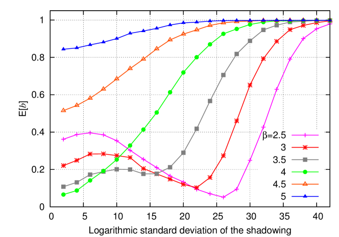
Various QoS metrics in cellular networks, as blocking probability for constant bit-rate (CBR) connections and spectral efficiency for variable bit-rate (VBR) connections, depend on the strength (i.e., variance) of the shadowing. It is commonly believed that an increase of the variance of shadowing penalizes the network performance. The results presented in this paper shed some new light on this problem. Namely, studying the blocking probability (defined as the fraction of the CBR connections that cannot be established due to insufficient transmission resources, in the long run of the system) we have discovered that it is not always increasing with the variance of the shadowing. For example, in our model of the OFDMA hexagonal network consisting of 36 BS, with cell radius $0.525$km and the path-loss exponent equal to $2.5$, the blocking probability evaluated at the presence of the log-normal shadowing with the standard deviation of 25dB is four times smaller than in the scenario with no-shadowing. Even if this spectacular example regards a very strong shadowing, we obtain a smaller, but still very significant, decrease of the blocking probability for the shadowing with the standard deviation from 7 to 15dB, which might be appropriate for the indoor scenario (user-indoors, BS-outdoors); cf [2].

In all cases, a very strong shadowing ultimately makes the blocking probability tend to 1 and this dependence indeed becomes (as expected) monotone for higher path-loss exponent (larger than 4 in the considered examples).

To explain the above, somewhat surprising, observations and extend them to other QoS metrics we study the impact of the shadowing and the path-loss exponent on the following two key characteristics of any given mobile in the network:

• its path-loss to the serving BS, which is the one received with the strongest signal (and not necessarily the closest one),

• the so called mobile’s interference factor, defined as the ratio of the sum of the path-gains form interfering BS to the path-gain from the serving BS.

These are two key ingredients in the analysis of wireless cellular networks and thus their mean values can be considered as some QoS “pre-metrics”. In particular, they are explicitly present in the call blocking condition — the one used to control the admission of streaming users, and hence intrinsically related to the blocking probability. They are, even more straightforwardly, related to the spectral efficiency of the data networks. While being key ingredients in the study of wireless systems, the (mean) QoS pre-metric are also more easy to analyse. In particular they do not depend on a particular assumption regarding the spatial correlation of shadowing (which is not the case, e.g. for the mean blocking probability).

We have studied the mean values of the above two basic QoS ingredients, with the averaging taken over all possible locations of users in the network and over the distribution of the shadowing.

Our main findings are as follows:

• The mean path-loss (with respect to the serving BS) is always increasing in the variance of the shadowing. The ultimate degradation of the QoS for large shadowing variance is due to this increasing path-loss. (When possible, this may be however remedied by increasing the power of the emitted signals).

• The mean interference factor is not monotonic in the variance of the shadowing. It first increases and then decreases (asymptotically to zero!), when the shadowing variance goes to infinity. This asymptotic behaviour can be heuristically explained by the single big jump principle of heavy-tailed distributions: the sum of the (log-normal) path-gains form all antennas is dominated by a big value of the path-gain from a single antenna. When this antenna is the serving one, then this big path-gain does not count in the interference, which becomes negligible in proportion to it.

• The above two facts lead to the phenomenon that we may call a stochastic resonance for QoS in path-loss-and-interference limited systems: when QoS is not yet compromised by path-loss conditions, a moderate increase of the shadowing variance may make it profit from the reduction of the interference.

We confirm the above findings by a mathematical analysis of the respective stochastic models. We also compare in this matter the performance of the perfect (hexagonal) and irregular (Poisson) networks and find that both architectures exhibit very similar QoS “pre-metrics” for the standard deviation of the shadowing larger than 20dB. Moreover, we prove an interesting invariance of the QoS metrics of the infinite Poisson cellular networks with respect to the distribution of the shadowing. As a consequence we also obtain fully explicit, analytical results for the mean path-loss and interference factors in the case of the infinite Poisson network.

The remaining part of this paper is organized as follows. In the next section we briefly present related works. In Section III we describe our models. The main numerical results are presented in Section IV. Next, in Section V we present mathematical analysis of the models, which supports and completes our numerical findings. Finally, in Section VI we provide some concluding remarks.

II Related works

The propagation loss model considered in this paper is commonly accepted in the literature; see e.g. [3] where log-normal shadowing of mean $1$ is considered. A possible extension of this model consists in assuming shadowing distribution (say, its variance) that depends on the distance, cf. [4].

The impact of the shadowing on the distribution of the interference factor is studied numerically in [5] and analytically in [6]. However, the above two articles do not take into account the modification of the network geometry induced by the shadowing, i.e., assume that mobiles are served by their geographically closest BS. This is not a realistic assumption and, as we will show in this paper, leads to misleading conclusions that the shadowing dramatically increases the mean interference factor.

The paper [7] focuses on the interference factor averaged over a given cell, and in particular the effect of shadowing on this average. It is shown there that the cell shape modification induced by the shadowing affects significantly the mean interference factor. More precisely, that this mean decreases substantially if mobiles are served by the BS offering the smallest path-loss. We adopt this assumption throughout the present paper in the context of regular (hexagonal) and irregular (Poisson) geometry of BS, as proposed in [8].

Some papers (see e.g. [9, 10]) propose more explicit approximations of the interference factor and its moments (mean and variance) assuming only deterministic propagation loss models (without random shadowing). [11] studies the distribution of the interference factor in such a case.

In [12] the authors partially confirm, by a different approach, our early observation from [1], that the average SIR (which is the inverse of the interference factor) might increase with the shadowing variance when the best server policy is chosen.

The interference factor was recognized very early as a key element in the performance evaluation of cellular networks; cf. [13, 14]. Fundamental to our approach to the evaluation of the blocking probability are papers [15, 16]. They show how the power allocation problem without power limitations can be reduced to an algebraic system of linear inequalities. Moreover, they recognize that the spectral radius of the (non-negative) matrix corresponding to this system not greater than 1 is the necessary and sufficient condition of the feasibility of power allocation without power limitations. This approach lead to the development of a comprehensive framework of the evaluation of the blocking probability in CDMA, HSDPA and OFDMA, via a spatial version of the famous Erlang’s formula in [17, 8, 18, 19]. QoS in data networks are studied using this approach in [20].

Finally, recalling that the mean QoS pre-metrics studied in this paper do not depend on the spatial correlation of the shadowing, we remind [21, 22] as bringing models that can be used when studying the spatial distribution of the QoS metrics.

III Model description

III-A Location of base stations

In this paper we will consider two particular models for the location of BS, hexagonal and Poisson one. The former is commonly considered as an “ideal” model for the cellular networks, while the latter one can be seen as an extremal case of very irregular network.

III-A1 Infinite Models

• Hexagonal network.

  

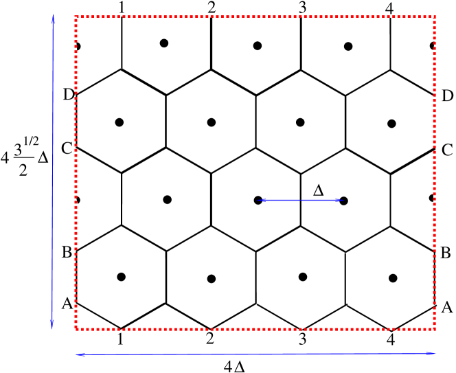
  Figure 1: Hexagonal pattern of $4\times 4$ BS on rectangular torus $\mathbb{T}_{4}$. Identified points are denoted by the same digits or characters.

  Consider BS located on a regular hexagonal grid on $\mathbb{R}^{2}$ with the distance $\Delta$ between two adjacent vertices of this grid ; cf. Figure 1. Note that the surface area of a given cell (hexagon, i.e. subset of the plane whose points are closer to a given point of the grid than to any other) of this model is equal to $\sqrt{3}\Delta^{2}/2$. Thus the intensity of the BS in this model is equal to $\lambda=2/(\sqrt{3}\Delta^{2})$ BS/$\text{km}^{2}$. In what follows it will be customary to consider a stationary version $\Phi_{H}$ of this grid, which can be obtained by randomly shifting it through a vector uniformly distributed in one given hexagon (cf. [23, Example 4.2.5]). In this model a given location, say the origin of the plane, corresponds to an “arbitrary” location of a mobile, “randomly chosen” in the network.

• Poisson network. Assume that BS are located at the points of a stationary, homogeneous Poisson point process (p.p.) $\Phi_{P}$ of intensity $\lambda$ BS/$\text{km}^{2}$ on the plane $\mathbb{R}^{2}$. When comparing performance of Poisson and hexagonal model we will always take them with the same intensity $\lambda=2/(\sqrt{3}\Delta^{2})$.

Considering infinite models is often a convenient way of studying phenomena arising in very large networks. A particular property of these models is lack of (geographic) boundary effects, which in real, large but finite, networks, have often a negligible impact on performance characteristics measured in the “middle” of the network. However, as we will see in this paper, sometimes mathematical assumption of an infinite network may create some artifacts, which are not observed in more realistic, large but finite, networks.

III-A2 Bounded Models

In order to have finite network models, and still neglect the boundary effects (which might be reasonable for large networks) one often considers toroidal model. Recall that, roughly speaking, rectangular torus is a rectangle whose opposite sites are “identified”. For $N=2,4,6,\ldots$, we will denote by $\mathbb{T}_{N}$ the rectangle $[-N\Delta/2,N\Delta/2)\times[-N\sqrt{3}\Delta/4,N\sqrt{3}\Delta/4)$ with toroidal metric. Restricting $\Phi_{H}$ to $\mathbb{T}_{N}$, i.e. taking $\Phi_{H}^{\mathbb{T}_{N}}=\Phi_{H}\cap\mathbb{T}_{N}$ one obtains the model whose distribution is invariant with respect to translations on the torus. Thus we obtain a hexagonal network model that consists of $N^{2}$ cells (cf. Figure 1) and which does not exhibit any border effects. Similarly we will consider the restriction $\Phi_{P}^{\mathbb{T}}$ of the Poisson p.p. $\Phi_{P}$ to $\mathbb{T}_{N}$.

III-B Path-loss model with shadowing

For a given BS $X\in\Phi$ ($\Phi=\Phi_{P}$ or $\Phi_{H}$) and a given location $y\in\mathbb{R}^{2}$ on the plane we denote by $L_{X}(y)$ the (time-average, i.e., averaged out over the fading) path-loss between BS $X$ and location $y$. In what follows we will always assume that

$$L_{X}(y)=\frac{L\left(\left|X-y\right|\right)}{S_{X}(y)}\,,$$ (1)

where $L(\cdot)$, called distance-loss, is a non-decreasing, deterministic function of the distance between an emitter and a receiver, and $S_{X}(\cdot)$ is a random shadowing field related to the BS $X$. In what follows we call $L_{X}(y)$ path-loss with shadowing (or path-loss for short) between $X$ and $y$. Moreover, we will always assume that given locations of BS $\{X_{i}\in\Phi\}$ their shadowing fields $\{S_{X_{i}}(\cdot)\}$ are independent non-negative stochastic processes, each being indexed by locations $y\in\mathbb{R}^{2}$. More formally speaking, the locations of BS $X$ and their respective shadowing fields $S_{X}(\cdot)$ form an independently marked version $\tilde{\Phi}=\{(X,S_{X}(\cdot))\}_{X\in\Phi}$ of the point process $\Phi$.

Regarding the distribution of the marks (shadowing fields) of this process, they are assumed to have the same marginal distributions, i.e., given $X$, $S_{X}(y)$ has the same distribution for all $y\in\mathbb{R}^{2}$, of normalized mean $\mathbf{E}[S_{X}(y)]=1$, with the following two cases being of particular interest

• $S_{X}(y)\equiv 1$, which corresponds to a case with negligible shadowing (we will say also “no shadowing”),

• for all $y$, $S_{X}(y)$ is log-nornal random variable with mean 1. Recall that such a mean-1 log-normal variable $S$ can be expressed as $S=e^{\mu+\sigma N}$ where $N$ is standard Gaussian random variable (with mean 0 and variance 1) with $\mu=-\sigma^{2}/2$ and some constant $\sigma$. Indeed, in this case $\mathbf{E}[S]=e^{\mu+\sigma^{2}/2}=1$. Note that if the shadowing is log-normal random variable then the path-loss (at a given distance) expressed in dB is Gaussian random variable. Furthermore, in this context it is common to parametrize the log-normal shadowing by the standard deviation (SD) of $S$ expressed in dB, i.e., the SD of $10\log_{10}S$. We will denote it by $v$. With respect to the previous parametrization we have $v=\sigma 10/\log 10$. Throughout the paper we will call $v$ the logarithmic standard deviation (log-SD) of the shadowing.

If not otherwise specified, we do not make any particular assumption on the correlation of the shadowing field $S_{X}(y)$ for given $X$ and different locations $y$.

Throughout the paper we will implicitly assume also that mean path-gain is finite, i.e., $\mathbf{E}[1/S]<\infty$. Note that this condition is satisfied for log-normal variable, indeed, in our case of mean-1 variable $\mathbf{E}[1/S]=e^{\sigma^{2}}=e^{v^{2}\log^{2}10/100}$.

For the deterministic distance-loss function $L(\cdot)$ the following particular model is often used and will be our default assumption in this paper:

$$L\left(r\right)=\left(Kr\right)^{\beta}$$ (2)

where $K>0$ and $\beta>2$ are some constants.

III-C Handover policy and path-loss factor

In what follows we will assume that each given location $y\in\mathbb{R}^{2}$ is served by the BS $X_{y}^{*}\in\Phi$ with respect to which it has the weakest path-loss $L_{X_{y}^{*}}(y)$ (so, in other words, the strongest received signal, given all BS emit with the same power), i.e, such that

$$L_{X_{y}^{*}}(y)\leq L_{X}(y)\qquad\text{for all\ }X\in\Phi\,,$$ (3)

with any tie-breaking rule. Note that in the case of negligible shadowing ($S_{X}(y)\equiv 1$) and strictly increasing function $L(\cdot)$ the above policy corresponds to the geographically closest BS. Note also that for our infinite network models with random shadowing, one has to prove that the minimum of the path-loss is achieved for some BS, i.e., that $X_{y}^{*}$ is well defined.

Note that $L_{X_{y}^{*}}(y)$ is the path-loss experienced by a user located at $y$ with respect to its serving BS. Obviously it determines the QoS of this user (we will be more specific on this in Section III-E). In this context we will call it path-loss factor of user $y$ and denote by $l(y)=L_{X_{y}^{*}}(y)$. Note that it depends on the location $y$ but also on the path-loss conditions of this location with respect to all BS in the network $l(y)=l(y,\tilde{\Phi})$. Path-loss factor $l(y)$ is typically not enough to determine the QoS of a given user.

III-D Interference factor

For a given location $y\in\mathbb{R}^{2}$ we define the interference factor $f(y)$ as

$$f(y)=f(y,\tilde{\Phi})=\sum_{X\in\Phi,X\not=X_{y}^{*}}\frac{L_{X_{y}^{*}}(y)}{L_{X}(y)}=\sum_{X\in\Phi}\frac{l(y)}{L_{X}(y)}-1$$ (4)

provided $X_{y}^{*}$ is well defined.

Study of the path-loss and interference factors, which are relatively simple objects, can give an important insight into more involved QoS metrics, such as blocking probability in streaming traffic and mean throughput in data traffic. In what follows we recall how $l(y)$ and $f(y)$ appear naturally in the evaluation of the blocking probabilities.

III-E Blocking probability; a space-time scenario

In this section we briefly describe the relation between the path-loss and interference factors and the blocking probability. This relation, whose very essence can be explained by the famous Erlang’s loss formula, was observed in the current geometric context (however without shadowing) in [18].

In order to evaluate the blocking probability it is necessary to specify the dynamics of call arrivals and their durations, as well as to identify the set of feasible configurations of users (which can be served simultaneously at their requested bit-rates). To this regard, consider a given realization of the netowrk with shadowing $\tilde{\Phi}$, and a spatio-temporal Poisson arrival process of calls which require from the network some predefined transmission rates for some exponential transmission times. These rates can be maintained at the price of blocking of some call arrivals when a network congestion occurs. The fractions $b=b(\tilde{\Phi})$ of blocked arrivals in the long run of the system is called the blocking probability. By the famous Erlang’s loss formula, it is equal to the conditional probability that in the stationary configuration of the (non-blocked) arrival process the system cannot admit a new user, given all users in the current configuration can be served. Moreover, if the decision whether to block a given call (or admit it) is based on the verification of some feasibility condition that has the so called multi-Erlang form, then the Erlang’s loss formula can be relatively easily evaluated, e.g. discretizing the values of the SINR and using Kaufman-Roberts algorithm. A canonical form of the multi-Erlang feasibility condition involves verification by each BS $X$ of the following condition

$$\sum_{y:X_{y}^{*}=X}\varphi\Bigl{(}l(y),f(y)\Bigr{)}\leq 1\,,$$ (5)

where the summation is taken over all users (including a new arrival) to be served by the BS $X$ and $\varphi(\cdot,\cdot)$ is some function of the path-loss and interference factors of user $y$. This condition guarantees sufficient wireless resources to maintain the predefined transmissions rates for all served mobiles. Specific form of the function $\varphi(\cdot,\cdot)$ needs to be developed for each particular cellular technology (taking into account the performance of the coding schemes, type of the multiplexing, etc.). Below we show two examples borrowed from our previous studies. They give some insight into how the feasibility condition (5) depends on the user transmissions rates, it is supposed to guarantee.

• For the down-link in the OFDMA network

  $$\varphi(l,f)=\frac{r}{W\psi\Bigl{(}(1-\epsilon)/((Nl/\tilde{P})+\alpha+f)\Bigr{)}}\,,$$ (6)

  where $\tilde{P}$ is the maximal BS power, $\epsilon$ is the fraction of this maximal power used in common (pilot) channels, $\alpha$ is the intra-cell orthogonality factor (usually assumed to be 0 in OFDMA), $N$ external noise power, $W$ is the system bandwidth, $r$ is the required bit-rate $r$ of user and $\psi$ is the link performance function ($\psi(\xi)$ is the bit-rate per Hz available when SINR is equal to $\xi$; ); cf. [19].

• For the down-link in CDMA network

  $$\varphi(l,f)=\frac{\xi}{1+\alpha\xi}\frac{1}{1-\epsilon}\Bigr{(}\frac{Nl}{\tilde{P}}+\alpha+f\Bigr{)}\,,$$ (7)

  where $\xi=\psi^{-1}(r/W)$ is the SINR threshold corresponding to the required bit-rate $r$ of user and the remaining notation notation as above; (cf. [18]).

In what follows we will denote by $\mathbf{E}[b]=\mathbf{E}[b(\tilde{\Phi})]$ the blocking probability averaged over possible scenarios regarding locations of BS and their shadowing conditions. It can be evaluated by the simulation of several realizations of the network with shadowing $\tilde{\Phi}$, evaluation of $b(\tilde{\Phi})$ by the Kaufman-Roberts algorithm as described above, and then taking the empirical average over the realizations of $\tilde{\Phi}$. However, in practice one realization of $\tilde{\Phi}$ is enough, provided the shadowing fields $S_{X}(y)$ do not exhibit high spatial correlation across $y$ ( recall that we have assumed them to be independent across $X$); cf. Footnote 4. Indeed, we have noticed in our experiments, that for large enough networks (in the case of the hexagonal network $\mathbb{T}_{6}$ is enough!) with spatially uncorrelated shadowing, the value of $b(\tilde{\Phi})$ is almost invariant with respect to $\tilde{\Phi}$ and hence very close to $\mathbf{E}[b(\tilde{\Phi})]$. This is due to spatial ergodic properties of the process $\tilde{\Phi}$.

III-F Our methodology in the study of the network QoS

In section IV-A we will show some numerical examples, which show the typical dependence of the blocking probability $\mathbf{E}[b]$ on the parameters of the path-loss model. These examples, restricted to OFDMA, are not supposed to be exhaustive. The goal is to show the typical tendencies.

In order to explain these tendencies, in Sections IV-B and IV-C we will study more thoroughly the mean values of the interference and path-loss factor $\mathbf{E}[f(y)]=\mathbf{E}[f(y,\tilde{\Phi})]$, $\mathbf{E}[l(y)]=\mathbf{E}[l(y,\tilde{\Phi})]$ (where the expectation $\mathbf{E}[\ldots]$ corresponds to the distribution of $\tilde{\Phi}$, i.e., this of the shadowing field and of the random location of the user). By the translation invariance of the distribution of our infinite and toroidal models, these expectations (corresponding the spatial averaging) do not depend on the user location and thus, for these models, $\mathbf{E}[l(y)]=\mathbf{E}[l(0)]$ and $\mathbf{E}[f(y)]=\mathbf{E}[f(0)]$ .

Our methodological conjecture is as follows. We believe that the mean path-loss and interference factors $\mathbf{E}[l(0)]$, $\mathbf{E}[f(0)]$ can be considered as primitive (basic) metrics of the QoS and their behavior can (at least qualitatively) explain the main tendencies observed for more involved QoS metrics. This methodological conjecture is motivated by the observation that the function $\varphi$ in the feasibility condition (5) is an increasing function of some linear combination of $l(y)$ and $f(y)$ (at least for the examples of CDMA and OFDMA given above). Indeed, we will show that the study of $\mathbf{E}[l(0)]$ and $\mathbf{E}[f(0)]$ can explain the aforementioned non-monotonicity of the blocking probability $\mathbf{E}[b]$ with respect to the standard deviation of the shadowing.

IV Numerical results

Following the methodology described in Section III-F, in this section we will first study the blocking probability and then the mean path-loss and interference factors for the hexagonal and Poisson network models with log-normal shadowing.

IV-A Blocking probability

In this section we consider only the hexagonal network on the torus $\mathbb{T}_{6}$. We evaluate the blocking probability $\mathbf{E}[b]$ in OFDMA network using the Kaufman-Roberts algorithm, as described in Section III-E.

We assume the following parameter values for OFDMA: System bandwidth $W=5$MHz. BS are equipped with omnidirectional antennas having a gain $9$dBi and transmit with the maximal power $43$dBm; thus $\tilde{P}=43+9=52$dBm when we account for the isotropic antenna gain. The common channel power is the fraction $\epsilon=0.12$ of $\tilde{P}$. The ambient noise power is assumed $N=-103$dBm.

We assume perfect intra-cell orthogonality, i.e., $\alpha=0$. Moreover we are not considering any opportunistic scheduling over fading. This allows us to characterize the link performance (averaged over fading) via the Shanon’s formula $r/W=\psi\left(\xi\right)=\log_{2}\left(1+\xi\right)$, without specifying into how many sub-carriers the bandwidth $W=5$MHz is split.

We assume a traffic demand of 46.2 Erlang per km² consisting of streaming calls at the bit-rate $r=180$Kbits/s (typical for videoconferencing) that is served by the hexagonal network consisting of 36 BS (on the tours $\mathbb{T}_{6}$) with the distance between adjacent BS $\Delta=1$km.

The (deterministic) distance-loss function is $L(x)=\left(Kx\right)^{\beta}$ with $K=8667$km^-1 (which follows from Cost-Hata model [26] for urban areas, assuming frequency 1795Mhz, BS antenna height 50m, mobile antenna height 1.5m, for $\beta=3.38$). Moreover, we assume that the values of the shadowing $S_{X}(y)$ for given $X$ and different locations $y$ are independent. Figure 2 shows the dependence of the blocking probability $\mathbf{E}[b]$ on the path-loss exponent $\beta$ and the logarithmic standard deviation $v$ of the log-normal shadowing evaluated in our OFDMA network model.

Figure 2: Blocking probability in OFDMA hexagonal network on the torus $\mathbb{T}_{6}$ with log-normal shadowing with log-SD $v$ and path-loss exponent $\beta$, evaluated using the Kaufman-Roberts algorithm for the traffic 46.2 Erlang per km².

Remark IV.1

• For negligible shadowing (logarithmic standard deviation close to 0) the blocking probability $\mathbf{E}[b]$ first decreases in the path-loss exponent $\beta$ (on our figures for $\beta$ from $2.5$ to 4) and then increases in $\beta$.

• The blocking probability is not always increasing in the standard deviation of the shadowing. Indeed, on our figures with $\beta\geq 4$ it is monotone increasing. However, for $\beta\leq 3.5$ the blocking probability $\mathbf{E}[b]$ first increases, then decreases, and ultimately increases to 1.

Note the decrease of the blocking probability in the standard deviation of the shadowing can be quite significant even between 7 and 15 dB, depending on the path-loss exponent.

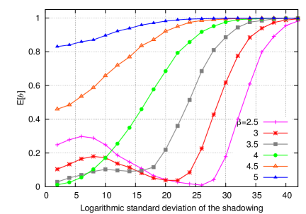
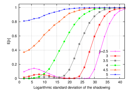
The lack of monotonicity observed in Remark IV.1 is not specific for our choice of the traffic of 46.2 Erlang par km² as can be remarked on Figure 3, where we have assumed two different smaller values of the traffic. Moreover, we have observed very similar patterns, not presented here due to space constraints, in our model of CDMA. Furthemore, we have confirmed these results by the the crude Monte-Carlo simulations of the network with the arrivals and departures of users (implemented in MATLAB).

(a) OFDMA, 34.6 Erlang per km²

(b) OFDMA, 23.1 Erlang per km²

Figure 3: Blocking probability for OFDMA network as on Figure 2 with traffic 34.6 Erlang per km² and 23.1 Erlang per km².

In the next section we will explain this behavior and argue that it my be expected for other QoS metrics which depend on some combination of the path-loss factor and the interference factor.

IV-B Analysis of the interference factor

Now, we will study the impact of the shadowing and also the geometry and size of the network on the interference factor $\mathbf{E}[f(0)]$ that is a key to the understanding of the strange non-monotonicity of the blocking probability shown above. Recall that, contrarily to the blocking probability, the expectation $\mathbf{E}[f(0)]$ (as well as $\mathbf{E}[l(0)]$) does not depend on any particular correlation of the values of the shadowing $S_{X}(y)$ for given $X$ and different locations $y$.

We begin with an important observation made directly from our model.

Remark IV.2

By the homothetic invariance of our hexagonal and Poisson models on the torus, or in the infinite models, with the distance-loss function (2), the mean interference factor does not depend on the intensity $\lambda$ of BS but only on the size $N$ of the network.

(a) hexagonal network

(b) Poisson network

Figure 4: Mean interference factor in hexagonal and Poisson network on the torus $\mathbb{T}_{N}$ with log-normal shadowing with log-SD $v$ and path-loss exponent $\beta$. Note that $\mathbf{E}[f(0)]$ increases with the size of the network. The straight lines correspond to the infinite (on $\mathbb{R}^{2}$) Poisson model; cf. Proposition V.6.

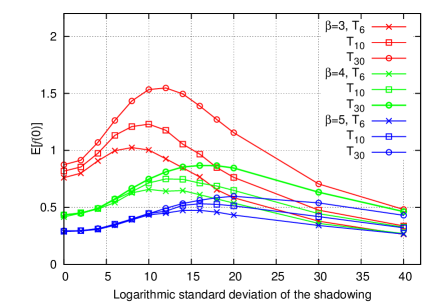
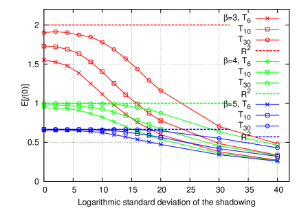
Figures 4(a) and 4(b) show the impact of the path-loss exponent, shadowing and the size of the network in the case of the hexagonal and Poisson network architecture, respectively. Here are our main observations.

Remark IV.3

1. Observe on Figure 4(a) for hexagonal network of a given size $N^{2}$ BS, with $N=6,10,30$, and a given path-loss exponent $\beta=3,4,5$, that the mean interference factor $\mathbf{E}[f(0)]$ first increases and then decreases to 0 when the value $v$ of logarithmic standard deviation (log-SD) of the shadowing increases.

2. For the Poisson network (see Figure 4(b)) $\mathbf{E}[f(0)]$ decreases in log-SD starting already from very small values of $v$.

3. The actual size of the network consisting of $N^{2}$ BS, when $N\geq 100$, has negligible impact on $\mathbf{E}[f(0)]$ when $\beta=4$ and $v\leq 10$ or $\beta=5$ and $v\leq 15$ both in hexagonal and Poisson case (in this latter case $N^{2}$ is the expected number of BS). In this regime the value of $\mathbf{E}[f(0)]$ corresponds to this in the respective infinite model. In particular, for Poisson network it is equal to $2/(\beta-2)$ and does not depend on log-SD $v$ (cf. Proposition V.6 below).

4. When $\beta=4$ and $v\geq 10$ or $\beta=5$ and $v\geq 15$ the mean interference factor $\mathbf{E}[f(0)]$ non-negligibly increases with the network size.

5. Comparing Figures 4(a) and 4(b) for $v\geq 20$ we observe that for large log-SD of the shadowing the mean interference factor evaluated for the Poisson network is almost exactly the same as for the hexagonal network of the same size.

Remark IV.4

The seminal paper [7] considers only the hexagonal network architecture, however, the beneficial impact of the shadowing is not observed there. The reason is that the model considered in [7] assumes that the smallest-path-loss BS (the serving one) is selected among the $N_{C}$ closest BS. In particular, $N_{C}=1$ ignores the shadowing in the handover policy as it corresponds to the situation where the serving BS is always the closest one. On the other hand the model considered in our paper corresponds to $N_{C}$ equal to the total number of BS in the network. In consequence, for a higher path-loss exponent (say $\beta=4$) and small and moderate log-SD of the shadowing ($0\leq v\leq 12$) our numerical results are close to those of [7] with $N_{C}=4$; cf. our Figure 4(a) and the last column in Table 1 in [7]. The fact that the average interference factor decreases in some cases with log-SD of the shadowing has not been observed in [7] due to the set of parameters considered there. Indeed, for a smaller path-loss exponent, $\beta=3$, our Figure 4(a) shows the mean interference factor decreasing in $v$ starting from $v\approx 8$. This range of parameters is also considered in [7, Table 2] however, with the $N_{C}=2$. Apparently the beneficial impact of the shadowing cannot be observed in this case, when the BS can be chosen only among two closest BS. A general remark is of the following order: strong shadowing requires larger geographical domain in which the serving BS is searched, as the optimal one may be located far from the mobile.

IV-C Analysis of the path-loss factor

(a) hexagonal network

(b) Poisson network

Figure 5: Mean path-loss factor expressed in dB, in hexagonal and Poisson network on the torus $\mathbb{T}_{N}$ with log-normal shadowing with log-SD $v$ and path-loss exponent $\beta$. Note that $\mathbf{E}[l(0)]$ decreases with the size of the network. The analytical expression for the infinite (on $\mathbb{R}^{2}$) Poisson model is given in Proposition V.6.

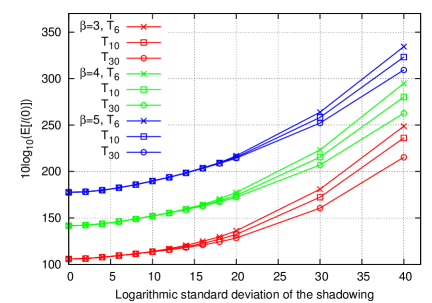
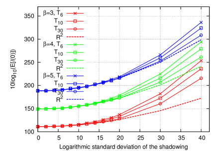
We begin with an important remark regarding the scaling of $\mathbf{E}[l(0)]$ with respect to the density of the BS.

Remark IV.5

Unlike the mean interference factor $\mathbf{E}[f(0)]$ (cf. Remark IV.2), the mean path-loss factor $\mathbf{E}[l(0)]$ depends on the intensity $\lambda$ of BS. By the homothetic invariance of our hexagonal and Poisson models, it is easy to see in the case of the distance-loss function (2) that this dependence has the following form $\mathbf{E}[l(0)]=\lambda^{-\beta/2}\Bigl{(}\mathbf{E}[l(0)]|_{\lambda=1}\Bigr{)}$. Consequently, in particular, the path-loss factor becomes preponderant in the case of sparse networks (small $\lambda$) and negligible for dense networks (large $\lambda$). We will see in Section V-B that $\mathbf{E}[l(0)]$ can be evaluated explicitly in the case of the infinite Poisson network with an arbitrary distribution of the shadowing.

Figures 5(a) and 5(b) show the mean path-loss factor $\mathbf{E}[l(0)]$ evaluated for the intensity of BS $\lambda=1.155$BS/km² (equivalent to $\Delta=1$km). The main observations are presented in the next section.

IV-D Conclusions on numerical results

For the hexagonal network we have observed the following facts regarding our two QoS “pre-metrics”.

• The mean path-loss factor increases to infinity in the standard deviation of the shadowing, increases in the path-loss exponent, increases in the cell radius, but (slightly) decreases in the number of base stations.

• The mean interference factor is not monotone in the standard deviation of the shadowing: first increases and then decreases to 0. It decreases in the path-loss exponent, is invariant with respect to the cell radius and increases in the number of base stations.

Knowing that the blocking probability depends on some combination of the path-loss and interference factors of users (cf. formulas (7) and (6)), and having observed that the mean values of these two factors have opposite monotonicities in the path-loss exponent, it is not surprising that the blocking probability is not monotone in the path-loss exponent; cf. the first observation of Remark IV.1. A similar argument explains a possible non-monotonicity of the blocking probability in the standard deviation of the shadowing; cf. the second observation of Remark IV.1 and the scheme on Figure 6.

Figure 6: Graphical explanation of a possible shape of the dependence of the blocking probability on the variance of the shadowing.

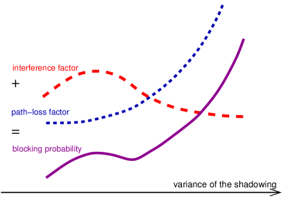
For the Poisson network we have observed the same tendencies of QoS “pre-metrics” as for hexagonal network mentioned above, except that the mean interference factor is monotone decreasing in the shadowing. Moreover, for large standard deviation of the shadowing, the “pre-metrics” of the Poisson network are very close to those of the hexagonal network.

In the next section we will prove also that for the infinite Poisson network the distributions of our QoS “pre-metrics” do not depend on the shadowing and admit explicit formulas for their means.

V Mathematical results

In this section we will state and prove some mathematical results regarding $\mathbf{E}[l(0)]$ and $\mathbf{E}[f(0)]$, which support and extend the numerical findings of Section IV.

V-A Toroidal models

We begin by a simple observation regrading the log-normal distribution of the shadowing $S$ with mean 1. Recall, it can be represented as $S=e^{-\sigma^{2}/2+\sigma N}$ where $N$ is the standard Gaussian random variable. Thus, for any fixed $\epsilon>0$ we have

$$\Pr\{S\geq\epsilon\} = \Pr\{N\geq\sigma/2+(\log\epsilon)/\sigma\}\buildrel\sigma\to\infty\over{\longrightarrow}0\,,$$

which shows that the random variable $S$ converges in probability to $0$ when $\sigma$ (and hence $v=\sigma 10/\log 10$) tends to infinity (and this even if $\mathbf{E}[S]\equiv 1$!). From this, we have that the path-loss between any location $y$ and any BS $X$, $L_{X}(y)=L(|X-y|)/S_{X}(y)$, converges in probability to infinity when the variance of the shadowing increases. Consequently, for any finite network $\tilde{\Phi}$ of base stations, the path-loss factor $l(y)=\min_{X\in\Phi}L_{X}(y)$ converges in probability and in expectation to infinity. This explains the asymptotics of $\mathbf{E}[l(0)]$ for large $v$ observed on Figures 5(a) and 5(b).

The somewhat surprising observation on Figures 4(a) and 4(b) regarding the beneficial impact of the strong log-SD $v$ of the shadowing on the mean interference factor can be also confirmed mathematically.

Proposition V.1

Assume an arbitrary, fixed, finite pattern $\{X_{1},X_{2},\ldots,X_{n}\}$ of BS locations. Consider any deterministic distance-loss function $0<L(r)<\infty$ and (independent) log-normal shadowing $S_{X_{i}}(\cdot)$ with the log-SD $v$. Then for any location $y$ we have $\lim_{v\to\infty}f(y)=0$ in probability.

Proof:

It is enough to show $\lim_{v\to\infty}\Pr\{\,f(y)\geq\epsilon\,\}=0$ for any $\epsilon$ satisfying $0<\epsilon<1$. Denote by $G_{i}=S_{X_{i}}(y)/L(|X_{i}-y|)$ the path-gain from $X_{i}$ to $y$. Consider ordered vector $(G_{(1)},\ldots,G_{(n)})$ of these path gains, where $\min_{i}G_{i}=G_{(1)}\leq\ldots\leq G_{(n)}=\max_{i}G_{i}$. Note that $f(y)=1/G_{(n)}\sum_{i=1}^{n}G_{(i)}-1\leq(n-1)G_{(n-1)}/G_{(n)}$. In order to prove our claim it is enough to show that $\Pr\{\,G_{(n-1)}/G_{(n)}\geq\epsilon\,\}\to 0$ when $v\to\infty$. To this regard denote $L(|X_{i}-y|)=l_{i}$, and recall from the definition of our path-loss model that we can represent $G_{i}(y)=e^{\tilde{N}_{i}}$, where $\{\tilde{N}_{i}\}_{i=1,\ldots,n}$ are independent Gaussian random variables, with mean $\mathbf{E}[\tilde{N}_{i}]=-\log l_{i}-\sigma^{2}/2$ and the same SD $\sigma=v\log 10/10$. Since $G_{i}$ is monotone increasing in $\tilde{N}_{i}$ we have $G_{(i)}=e^{\tilde{N}_{(i)}}$, where $\min_{i}\tilde{N}_{i}=\tilde{N}_{(1)}\leq\ldots\leq\tilde{N}_{(n)}=\max_{i}\tilde{N}_{i}$. Moreover, $A:=\{\,G_{(n-1)}/G_{(n)}\geq\epsilon\,\}=\{\,\tilde{N}_{(n)}-\tilde{N}_{(n-1)}\leq M\,\}$, where $M=-\log\epsilon$. Denote by $A_{ij}=\{\,0\leq\tilde{N}_{i}-\tilde{N}_{j}\leq M\,\}$. Note that $A\subset\bigcup_{i,j=1,\ldots,n,i\not=j}A_{ij}$ and the result follows from the fact that for any $i\not=j$ $\Pr\{A_{ij}\}\to 0$ when $v\to\infty$. Indeed, for $i\not=j$, $\tilde{N}_{i}-\tilde{N}_{j}=\bar{N}$ is Gaussian random variable with mean $\log(l_{j}/l_{i})$ and variance $\sigma^{2}$ and thus $\Pr\{A_{ij}\}=\Pr\{\,0\leq\bar{N}\leq M\}\to 0$ for any given finite $M$ when $\sigma^{2}=v^{2}\log^{2}10/100\to\infty$. This completes the proof. ∎

Corollary V.2

Assume Poisson or hexagonal network on the torus $\mathbb{T}_{N}$, with log-normal shadowing having log-SD $v$. Then the mean interference factor $f(0)$ converges in distribution and in expectation to 0 when $v\to\infty$.

Proof:

For any $\epsilon>0$, by Proposition V.1 and Lebesgue dominated convergence theorem we have $\Pr\{\,f(0,\tilde{\Phi})>\epsilon\,\}=\mathbf{E}[\Pr\{\,f(0,\tilde{\Phi})>\epsilon\,|\Phi\}]\to 0$, when $v\to\infty$. This proves that $f(0)$ converges in distribution to 0. Convergence of $\mathbf{E}[f(0)]$ to 0 follows again from the Lebesgue dominated convergence theorem by the observation $f(y,\tilde{\Phi})\leq\Phi(\mathbb{T}_{N})-1$ and $\mathbf{E}[\Phi(\mathbb{T}_{N})]<\infty$. ∎

Remark V.3

Recall that the log-normal distribution of the shadowing is heavy-tailed. The result of Proposition V.1 and Corollary V.2 can be heuristically explained and conjectured for other heavy tailed shadowing distributions by the so called single big jump principle, cf e.g. [27, Section 3.1]. It says that the only significant way in which a large value of the sum of independent heavy-tailed variables can be attained is through a big value of single term of the sum (“big jump”). In other words, the maximum and the sum of independent heavy-tailed random variables have the same asymptotic of the distribution function for large values. Note also, that we observe the “single big jump principle” in a different scenario: we study the ratio of the interference (sum of the log-normal path-gains minus the largest path-gain) to the serving-BS path-gain (the largest one) asymptotically for large variance.

V-B Infinite models

In this section we will consider infinite hexagonal and Poisson models. We will show first that serving BS $X_{0}^{*}$, and hence the path-loss and interference factors, are well defined. Then we will argue that values of these factors in the infinite models can be seen as limits of respective toroidal models on $\mathbb{T}_{N}$ when $n\to\infty$. Finally we will prove a (surprising?) invariance of $\mathbf{E}[l(0)]$ and $\mathbf{E}[f(0)]$ in the infinite Poisson model with respect to the distribution of the shadowing. In this case the values $\mathbf{E}[l(0)]$ and $\mathbf{E}[f(0)]$ can be evaluated explicitly.

Proposition V.4

Consider infinite Poisson $\Phi=\Phi_{P}$ or hexagonal $\Phi=\Phi_{H}$ model of BS, with shadowing whose marginal distribution has finite moment of order $2/\beta$ (). Then there exist $X_{0}^{*}\in\Phi$ satisfying (3). Moreover, the path-loss factor and the interference factor calculated with respect to the restriction of $\Phi$ to $\mathbb{T}_{N}$, i.e., $l(0,\tilde{\Phi}^{\mathbb{T}_{N}})$ and $f(0,\tilde{\Phi}^{\mathbb{T}_{N}})$, converge almost surely and in expectation to $l(0,\tilde{\Phi})$ and $f(0,\tilde{\Phi})$, respectively.

Proof:

To prove the first statement it is enough to show that the expected number of BS $X_{i}$ such that $S_{X_{i}}(0)/L(|X_{i}|)>M$ is finite for any $M<\infty$. In the case of the Poisson p.p. this will be shown in the proof of Proposition V.6 below. Here we consider only hexagonal case $\Phi=\Phi_{H}$. Denote by $\overline{G}(x)=\Pr\{\,S>x\,\}$. We have

$$\mathbf{E}[\#\{X_{i}\in\Phi_{H}:S_{X_{i}(0)}/L(|X_{i}|)>M\}]$$

$$= \mathbf{E}\Bigl{[}\sum_{X_{i}\in\Phi_{H}}\mathds{1}\Bigl{(}S_{X_{i}(0)}>ML(|X_{i}|)\Bigr{)}\Bigr{]}$$

$$= \mathbf{E}\Bigl{[}\sum_{X_{i}\in\Phi_{H}}\overline{G}\Bigl{(}ML(|X_{i}|)\Bigr{)}\Bigr{]}$$

$$\leq \sum_{i=1}^{\infty}6n\overline{G}\Bigl{(}(n\Delta K/2)^{\beta}/M\Bigr{)}<\infty,$$

where $\mathds{1}(\cdot)$ denotes the indicator function and the last inequality follows from the assumption $\mathbf{E}[S^{2/\beta}]=2/\beta\int_{0}^{\infty}s^{2/\beta-1}\overline{G}(s)\,ds<\infty$. This completes the proof of the first statement.

In order to prove the second statement, note that for any realization the network $\tilde{\Phi}$, for $N$ large enough $X_{0}^{*}\in\mathbb{T}_{N}$. Consequently, $l(0,\tilde{\Phi}^{\mathbb{T}_{N}})$ is eventually constant in $N$ while $f(0,\tilde{\Phi}^{\mathbb{T}_{N}})$ eventually increases in $N$ (the serving BS is not changing any more and only interference is added). The convergence of the expectation of the path-loss factor follows from the monotone convergence theorem, noting that $l(0,\tilde{\Phi}^{\mathbb{T}_{N}})$ is decreasing in $N$. The convergence of the expectation of the interference factor follows form the dominated convergence theorem knowing that $f(0,\tilde{\Phi})\leq f^{\prime}(0,\tilde{\Phi})$, where $f^{\prime}(0,\tilde{\Phi})$ is the interference factor calculated under assumption that the handover policy selects the geographically closest BS as the serving one. By the independence of the shadowing fields given the locations of BS and the assumption that the mean shadowing is equal to 1

$$\mathbf{E}[f^{\prime}(0,\tilde{\Phi})]=\mathbf{E}\Bigl{[}\frac{1}{S}\Bigr{]}\mathbf{E}\Bigl{[}\sum_{X\in\Phi}\frac{L(|X_{0}^{{}^{\prime}*}|)}{L(|X|)}\Bigr{]}-1\,,$$ (8)

where $X_{0}^{{}^{\prime}*}$ is a point of $\Phi$ closest to the origin 0. By our assumption on the mean path-gain $\mathbf{E}[1/S]<\infty$. The second expectation (8) is equal to the mean interference factor in the infinite model with constant shadowing $S\equiv 1$, and it is known to be finite in the infinite hexagonal and Poisson model; cf. respectively Remark V.5 and Proposition V.6 below. ∎

Remark V.5

It was shown in [8] that in the case of $S\equiv 1$ and the deterministic distance-loss function (2) $\mathbf{E}[l(0)]$ and $\mathbf{E}[f(0)]$ in the hexagonal model can be approximated by the following expressions

$$\mathbf{E}[f(0,\Phi_{H})] \approx \frac{0.9365}{\beta-2},$$

$$\mathbf{E}[l(0,\Phi_{H})] \approx \frac{K^{\beta}}{(\pi\lambda)^{\beta/2}(1+\beta/2)}\,.$$

To the best of our knowledge, analytical expressions (approximations) in the case of the infinite hexagonal network with random shadowing are not known. We consider now infinite Poisson model.

Proposition V.6

Assume infinite Poisson network, deterministic distance-loss function (2) and a general distribution of the shadowing $S$ satisfying $\mathbf{E}[S^{2/\beta}]<\infty$. Then the distribution of the interference factor $f(0)=f(0,\tilde{\Phi})$ does not depend on the distribution $S$ and the distribution of $l(0)$ depends on $S$ only through the product $\lambda\mathbf{E}[S^{2/\beta}]$. Moreover

$$\mathbf{E}[f(0)] = \frac{2}{\beta-2}\,,$$

$$\mathbf{E}[l(0)] = \frac{K^{\beta}\Gamma(1+\beta/2)}{(\pi\lambda\mathbf{E}[S^{2/\beta}])^{\beta/2}}\,,$$

where $\Gamma(a)=\int_{0}^{\infty}t^{a-1}e^{-t}dt$. In particular, for the log-normal shadowing

$$\mathbf{E}[l(0)]=\frac{K^{\beta}\Gamma(1+\beta/2)\exp[(1-2/\beta)\sigma^{2}/2]}{(\pi\lambda)^{\beta/2}}\,.$$

Remark V.7

The above result says that in the infinite Poisson notwork the existence of shadowing has no impact on the mean interference factor. The impact of the shadowing on the mean path-loss factor in this model consists in a “fictitious” scaling of the intensity of the BS by the factor $(\mathbf{E}[S^{2/\beta}])^{\beta/2}\leq 1$. The respective expressions in the case of $S\equiv 1$ has been found for the first time (to the best of our knowledge) in [17]. Note however, that the above observation is valid only if the handover policy selects the BS with the smallest path-loss, as described in Section III-C. Indeed, assume that, despite non-constant shadowing, the handover policy selects the geographically closest BS as the serving one. Then, the mean interference factor $\mathbf{E}[f^{\prime}(0)]$ can be expressed as in (8). Recall that the second expectation in this expression is equal to the mean interference factor in the same model without shadowing (i.e., $S\equiv 1$). By the Jensen’s inequality $\mathbf{E}[1/S]\geq 1/\mathbf{E}[S]=1$ and consequently we observe the increase of the mean interference factor compared to the “shadowing-dependent” handover policy. In particular, for log-normal $S$ with mean 1 and log-SD  $v$ we have $\mathbf{E}[1/S]=e^{\sigma^{2}}=e^{v^{2}\log^{2}10/100}$, which means that the log-normal shadowing in any geometric model of BS in which it is not taken into account in the handover policy increases the mean interference factor by $v^{2}\log 10/10\,$dB, where $v$ is log-SD of the shadowing.

Proof:

Note that the values of $l(0)$ and $f(0)$ are entirely defined by the collection of random variables $\{L_{X}(0)=L(|X|)/S_{X}(0):X\in\Phi\}$. Given $\Phi$ these random variables are independent. Thus by the displacement theorem for Poisson p.p. (cf. [23, Theorem 1.3.9]) $\{L_{X}(0)\}=\Psi$ constitutes a (non-homogeneous) Poisson p.p. on $\mathbb{R}^{+}=[0,\infty)$ of intensity measure $\Lambda^{\prime}$ given by

$$\Lambda^{\prime}([0,s]) = \mathbf{E}[\Psi([0,s])]$$

$$= \lambda\int_{\mathbb{R}^{2}}\Pr\{\,L(|z|)/S\leq s\,\}\,dz$$

$$= 2\pi\lambda\int_{0}^{\infty}r\Pr\{\,L(r)/S\leq s\,\}\,dr$$

$$= 2\pi\lambda\int_{0}^{\infty}r\mathbf{E}\left[\mathds{1}\left(L(r)/S\leq s\right)\right]\,dr$$

$$= 2\pi\lambda\mathbf{E}\left[\int_{0}^{(sS)^{1/\beta}/K}r\,dr\right]$$

$$= \frac{\lambda s^{2/\beta}\pi}{K^{2}}\mathbf{E}\left[S^{\frac{2}{\beta}}\right]\,.$$

Note that the latter expression is finite, which proves that the serving BS $X_{0}^{*}$ is well defined (cf. proof of Proposition V.4). Note also that it depends on the shadowing only through its moment $\mathbf{E}[S^{2/\beta}]$. Moreover one obtains the same expression in the model without shadowing and the density of BS multiplied by $\mathbf{E}[S^{2/\beta}]$. By the homothetic invariance of the Poisson model with the distance-loss function (2) the distribution of $f(0)$ does not depend on the intensity of the BS. Thus the invariance of the distribution of $f(0)$ on the distribution of the shadowing. In particular, we can conclude that $\mathbf{E}[f(0)]=2/(\beta-2)$ — the value obtained in the model without shadowing; see [17], cf. also [23, Example 4.5.1]. The formula for the mean path-loss factor follows from its dependence on the intensity of the base stations via the function $\lambda^{-\beta/2}$. This completes the proof. ∎

VI Concluding remarks

We show that the QoS in path-loss-and-interference limited cellular networks is not always decreasing in the strength (variance) of the log-normal shadowing, provided the handover policy selects the BS with the smallest path-loss as the serving one. Under strong shadowing it principally suffers from the poor path-loss conditions with respect to the serving BS. For moderate shadowing however, when the QoS is not yet compromised by the path-loss conditions, it may profit from the reduction of the interference. This is because increasing variance of the log-normal shadowing tends to “separate” the strongest (serving BS) signal from all other signals — the phenomenon observed for heavy-tailed distributions and called “single big jump principle”. This mathematical result seems also to be in line with a recent real-network observation [28] that mobiles in indoor communications (typically subject to strong shadowing) report fewer BSs for potential handover. The results presented in this paper regard the network-average of the QoS metrics. More study is needed, to analyze the impact of the shadowing on the distribution of these metrics in the network. This requires appropriate models of the spatial correlation of the shadowing.

References

- [1] B. Błaszczyszyn, M. K. Karray, and F.-X. Klepper, “Impact of the geometry, path-loss exponent and random shadowing on the mean interference factor in wireless cellular networks,” in Proc. of IFIP WMNC, Budapest, Hungary, 2010.
- [2] B. Błaszczyszyn and M. Karray, “Linear-regression estimation of the propagation-loss parameters using mobiles’ measurements in wireless cellular network,” in Proc. of WiOpt, 2012, see also http://hal.inria.fr/hal-00661248.
- [3] G. Stüber, Principle of Mobile Communication. Dordrecht, Netherlands: Springer, 2001.
- [4] Y. Liang, A. Goldsmith, G. Foschini, R. Valenzuela, and D. Chizhik, “Evolution of base stations in cellular networks: Denser deployment versus coordination,” in Proc. of ICC, 2008.
- [5] A. Masmoudi and S. Tabbane, “Other-cell-interference factor distribution model in downlink WCDMA systems,” in Proc. of MSWiM ’04. ACM, 2004.
- [6] J. M. Kelif and M. Coupechoux, “Impact of topology and shadowing on the outage probability of cellular networks,” in Proc. of IEEE ICC, 2009.
- [7] A. Viterbi, A. Viterbi, and E. Zehavi, “Other-cell interference in cellular power-controlled CDMA,” IEEE Trans. Commun., vol. 42, Mar. 1994.
- [8] F. Baccelli, B. Błaszczyszyn, and M. Karray, “Up and downlink admission/congestion control and maximal load in large homogeneous CDMA networks,” MONET, vol. 9, no. 6, Dec. 2004.
- [9] J. Kelif, M. Coupechoux, and P. Godlewski, “Fluid model of the outage probability in sectored wireless networks,” in Proc. of WCNC, 2008, pp. 2933–2938.
- [10] M. Karray, “Study of a key factor for performance evaluation of wireless cellular networks: The f-factor,” in Proc. of IFIP Wireless Days, Dec. 2009.
- [11] D. Staehle, K. Leibnitz, K. Heck, B. Schröder, A. Weller, and P. Tran-Gia, “Approximating the othercell interference distribution in inhomogeneous UMTS networks,” in Proc. of VTC, 2002.
- [12] M. Minelli, M. Coupechoux, and J.-M. Kelif, “Average sir estimation in cellular networks with best server policy,” in Wireless Days (WD), 2010 IFIP, 2010, pp. 1–5.
- [13] A. Viterbi and A. Viterbi, “Erlang capacity of a power controlled CDMA system,” IEEE J. Select. Areas Commun., vol. 11, no. 6, Aug. 1993.
- [14] J. Lee and L. Miller, CDMA systems engineering handbook. Boston: Artech House, 1998.
- [15] J. Zander, “Performance of optimum transmitter power control in cellular radio systems,” IEEE Trans. Veh. Technol, vol. 41, no. 1, 1992.
- [16] ——, “Distributed co-channel interference control in cellular radio systems,” IEEE Trans. Veh. Technol, vol. 41, 1992.
- [17] F. Baccelli, B. Błaszczyszyn, and F. Tournois, “Downlink admission/congestion control and maximal load in CDMA networks,” in Proc. of IEEE INFOCOM, 2003.
- [18] F. Baccelli, B. Błaszczyszyn, and M. Karray, “Blocking Rates in Large CDMA Networks via Spatial Erlang Formula,” in Proc. of IEEE INFOCOM, 2005.
- [19] B. Błaszczyszyn and M. Karray, “Dimensioning of the downlink in OFDMA cellular networks via an Erlang’s loss model,” in Proc. of European Wireless, 2009.
- [20] B. Błaszczyszyn and M. K. Karray, “Performance evaluation of scalable congestion control schemes for elastic traffic in cellular networks with power control,” in Proc. of IEEE INFOCOM, May 2007.
- [21] M. Gudmundson, “Correlation model for shadow fading in mobile radio systems,” Electronics Letters, vol. 27, no. 23, 1991.
- [22] T. Klingenbrunn and P. Mogensen, “Modelling cross-correlated shadowing in network simulations,” IEEE VTC, pp. 1407–1411, 1999.
- [23] F. Baccelli and B. Błaszczyszyn, Stochastic Geometry and Wireless Networks, Volume I — Theory, ser. Foundations and Trends in Networking. NoW Publishers, 2009, vol. 3, No 3–4.
- [24] A. Goldsmith and S.-G. Chua, “Variable-rate variable-power MQAM for fading channels,” IEEE Trans. Commun., vol. 45, pp. 1218–1230, 1997.
- [25] I. E. Telatar, “Capacity of multiple antenna Gaussian channels,” AT&T Technical Memorandum, June 1995.
- [26] COST 231, Evolution of land mobile radio (including personal) communications, Final report, Information, Technologies and Sciences, European Commission, 1999.
- [27] S. Foss, D. Korshunov, and S. Zachary, An Introduction to Heavy-Tailed and Subexponential Distributions, ser. Springer Series in Operations Research and Financial Engineering. Springer, 2011.
- [28] N. Malhouroux, private communication, Orange Labs, 2011.