Effects of anchored flexible polymers on mechanical properties of model biomembranes

Abstract

We have studied biomembranes with grafted polymer chains using a coarse-grained membrane simulation, where a meshless membrane model is combined with polymer chains. We focus on the polymer-induced entropic effects on mechanical properties of membranes. The spontaneous curvature and bending rigidity of the membranes increase with increasing polymer density. Our simulation results agree with the previous theoretical predictions.

I INTRODUCTION

Cellular membranes in living cells are a complex and compound system, including various kinds of proteins and different lipid compositions. Some of them are ”decorated” by sugar chains called glycoproteins or glycolipids A:Alberts2007 ; A:LipSac1995 . From theoretical and experimental aspects, pure lipid membrane in tensionless fluidic state has extensively received much attention for a long time A:Seifert1997 . Pioneer studies on the polymer-membrane compound system, especially on membrane with anchored polymers, have been recently reported by several groups both theoretically and experimentally A:Li1995 ; A:Li1996 ; A:Auth2003 ; A:HG1999 . They found that the mechanical properties of lipid membrane, such as the bending rigidity $\kappa$, the saddle-splay modulus $\bar{\kappa}$, and the spontaneous curvature $c_{0}$, can be dramatically changed by the interaction between membrane and the surrounding solvent and macromolecules A:LiPA1998 ; A:LiHG1998 . Liposomes decorated by grafted polymers (PEG etc.) are often used for carriers in drug delivery systems A:Needham1992 ; A:Allen2002 . Thus, it is important to understand the effects of grafted polymers for both fundamental research and medical applications.

In this paper, we explain our simulation model and then briefly describe the effects of grafted polymers on membrane properties. We employed a meshless membrane model with grafted polymer chains, since it allows large scale simulations and the mechanical properties of pure membranes are easy to control A:nog09 ; A:Hiro2006 . For an isolated anchored polymer chain, the membrane properties have been investigated in details by using scaling analysis and partition function method A:Li1995 ; A:Li1996 ; A:Auth2003 . Here we focus on membranes with a high polymer density, where the interactions between polymer chains are not negligible and have significant effects.

II model and method

Figure 1: A coarse-grained lipid membrane anchored with a coarse-grained polymer chain to form a grafted biomembrane system. The dark-gray particle represent membrane particles. A single polymer chain is composed of ten (light-gray) particles which are freely linked as an excluded-volume chain.

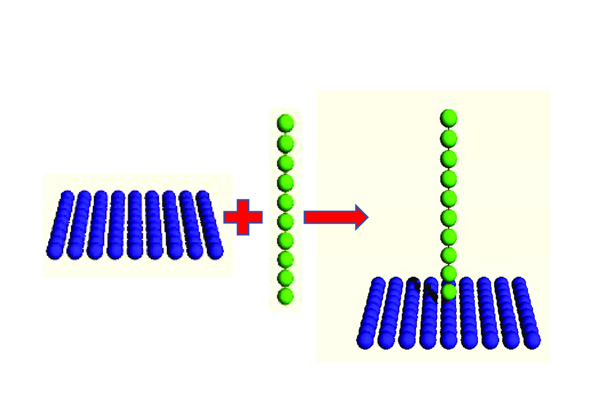
In this work, we employ a coarse-grained lipid membrane grafted with a coarse-grained flexible linear polymer chain to form a grafted biomembrane system (see Fig. 1). One membrane particle represents a patch of bilayer membrane, and possesses only transnational degree of freedom. The particles form a quasi-2D membrane by a curvature potential based on moving least-squares (MLS) method A:Hiro2006 . (ii) Polymer particles are linked by a harmonic potential, and freely move like a bead-spring behavior with a soft-core repulsion. An end of each polymer chain is anchored on one membrane particle with the harmonic potential.

We consider a patch of membrane composed of $N_{\rm{mb}}$ membrane particles. Among them, $N_{\rm{chain}}$ membrane particles are anchored by a polymer chain. Each polymer chain consists of $N_{\rm{p}}$ polymer segments with a connected membrane particle. The membrane and polymer particles interact with each other via a potential

$$U_{\rm{tot}}=U_{\rm{rep}}+U_{\rm{mb}}+U_{\rm{p}}.$$ (1)

All particles have a soft-core excluded volume term with a diameter of $\sigma$.

$$U_{\rm{rep}}=\varepsilon\sum_{i<j}\exp\left[-20(r_{ij}/\sigma-1)+B\right]f_{\rm{cut}}(r_{ij}/\sigma)$$ (2)

which $r_{ij}$ is the distance between membrane (or polymer) particles $i$ and $j$. The diameter $\sigma$ is used as the length unit, $B=0.126$, and $f_{\rm{cut}}(s)$ is a $C^{\infty}$ cutoff function

$$f_{\rm{cut}}(s)=\left\{\begin{array}[]{ll}\exp\left\{A\left[1+\frac{1}{(|s|/s_{\rm{cut}})^{n}-1}\right]\right\}&(s<s_{\rm{cut}})\\ 0&(s\geqslant s_{\rm{cut}})\end{array}\right.$$ (3)

with $n=12$. The factor $A$ in Eq. $(3)$ is determined so that $f_{\rm{cut}}(s_{\rm{half}})=0.5$, which implies $A=\ln(2){(s_{\rm{cut}}/s_{\rm{half}})^{n}-1}$. In Eq. $(2)$, we use the parameters $A=1$, and $s_{\rm{cut}}=1.2$.

II.1 Meshless membrane model

The membrane potential $U_{\rm{mb}}$ consists of attractive and curvature potentials,

$$U_{\rm{mb}}=\varepsilon\sum_{i}^{N_{\rm{mb}}}U_{\rm{att}}(\rho_{i})+k_{\alpha}\alpha_{\rm{pl}}({\mathbf{r}}_{i}),$$ (4)

where the summation is taken only over the membrane particles. The attractive multibody potential is employed to mimic the ”hydrophobic” interaction.

$$U_{\rm{att}}(\rho_{i})=0.25\ln\left\{1+\exp\left[-4(\rho_{i}-\rho^{\ast})\right]\right\}-C,$$ (5)

which is a function of the local density of membrane particles

$$\rho_{i}=\sum_{j\neq i}^{N_{\rm{mb}}}f_{\rm{cut}}(r_{ij}/\sigma),$$ (6)

with $n=12$, $s_{\rm{half}}=1.8$ [satisfied with $f_{\rm{cut}}(s_{\rm{half}})=0.5$], and $s_{\rm{cut}}=s_{\rm{half}}+0.3$. The constant $C=0.25\ln\left[1+\exp(4\rho^{\ast})\right]$ is chosen so that $U_{\rm{att}}=0$ at $\rho_{i}=0$. Here we set $\rho^{\ast}=6$ in order to simulate 2D fluidic membrane. For $\rho_{i}<\rho^{\ast}$, $U_{\rm{att}}$ acts like a pairwise potential with $U_{\rm{att}}=-2\sum_{j>i}f_{\rm{cut}}(r_{ij}/\sigma)$. For $\rho_{i}\gtrsim\rho^{\ast}$, this potential saturates to the constant $-C$. Thus, it is a pairwise potential with a cutoff at higher densities than $\rho^{\ast}$.

The curvature potential is given by the shape parameter called ”aplanarity”, which is defined by

$$\alpha_{\rm{pl}}=\frac{9D_{\rm{w}}}{T_{\rm w}M_{\rm w}},$$ (7)

with the determinant $D_{\rm w}=\lambda_{1}\lambda_{2}\lambda_{3}$, the trace $T_{\rm w}=\lambda_{1}+\lambda_{2}+\lambda_{3}$, and the sum of principal minors $M_{\rm w}=\lambda_{1}\lambda_{2}+\lambda_{2}\lambda_{3}+\lambda_{3}\lambda_{1}$. The aplanarity $\alpha_{\rm{pl}}$ scales the degree of deviation from the planar shape, and $\lambda_{1}$, $\lambda_{2}$, $\lambda_{3}$ are three eigenvalues of the weighted gyration tensor

$$a_{\alpha\beta}({\mathbf{r}}_{i})=\sum_{j}^{N_{\rm{mb}}}(\alpha_{j}-\alpha_{G})(\beta_{j}-\beta_{G})w_{\rm{cv}}(r_{ij}),$$ (8)

where $\alpha,\beta\in\left\{x,y,z\right\}$. Without loss of generality, we suppose $\lambda_{1}\leqslant\lambda_{2}\leqslant\lambda_{3}$. If $\lambda_{1}$ is the minimum eigenvalue representing a relative deviation from the local plane patch formed by the neighbor membrane particles around, its corresponding eigenvector is collinear with the normal vector $\mathbf{n}$ of this plane patch. When the $i$-th membrane particle has two or less neighbor particles within the cutoff distance $r_{\rm{cc}}$, they could be localized on a certain plane, therefore $\alpha_{\rm{pl}}=0$. The mass center of local plane patch $\mathbf{r}_{G}=\sum_{j}\mathbf{r}_{j}w_{\rm{cv}}(r_{ij})/\sum_{j}w_{\rm{cv}}(r_{ij})$, where a Gaussian $C^{\infty}$ cutoff function is employed to calculate the weight of the gyration tensor

$$w_{\rm{cv}}(r_{ij})=\left\{\begin{array}[]{ll}\exp\left[\frac{(r_{ij}/r_{\rm{ga}})^{2}}{(r_{ij}/r_{\rm{cc}})^{n}-1}\right]&(r_{ij}<r_{cc})\\ 0&(r_{ij}\geqslant r_{\rm{cc}}),\end{array}\right.$$ (9)

which is smoothly cut off at $r_{ij}=r_{\rm{cc}}$. Here we use the parameters $n=12$, $r_{\rm{ga}}=0.5r_{\rm{cc}}$, and $r_{\rm{cc}}=3\sigma$. The bending rigidity and the line tension of membrane edges are linearly dependent on $k_{\alpha}$ and $\varepsilon$, respectively, for $k_{\alpha}\gtrsim 10$, so that they can be independently varied by changing $k_{\alpha}$ and $\varepsilon$, respectively. As described in the previous work A:Hiro2006 , the aplanarity $\alpha_{\rm{pl}}\simeq 9\lambda_{1}/\left(\lambda_{2}+\lambda_{3}\right)$ for the smallest eigenvalue $\lambda_{1}\ll\lambda_{2}$,$\lambda_{3}$. Locally a membrane patch can be expressed for small fluctuations in the Monge representation as

$$z=z_{0}+\frac{1}{2}C_{1}(x-x_{0})^{2}+\frac{1}{2}C_{2}(y-y_{0})^{2},$$ (10)

where $x$ and $y$ coordinates are set to the principal axes. $C_{1}$ and $C_{2}$ are the principal curvatures of the membrane patch. In the case of cylindrical membrane, $C_{1}=1/R$ and $C_{2}=0$. By averaging over the local neighborhood with a weight function $w(r)$ where $r^{2}=x^{2}+y^{2}$, we have

$$\lambda_{1}=\langle z^{2}\rangle-\langle z\rangle^{2}=(C_{1}^{2}+C_{2}^{2})\langle(r^{2}-\langle r^{2}\rangle)^{2}\rangle.$$ (11)

Since $C_{1}^{2}+C_{2}^{2}=(C_{1}+C_{2})^{2}-2C_{1}C_{2}$, we easily know

$$k_{\alpha}\alpha_{\rm{pl}}\sim k_{\alpha}\lambda_{1}\sim k_{\alpha}(C_{1}+C_{2})^{2}.$$ (12)

Thus, a linear relation between the bending energy in Helfrich’s macroscopic model and our mesoscopic parameter is obtained as $\kappa\propto k_{\alpha}$, which is numerically confirmed in the previous work A:Hiro2006 ; A:Hay2011 .

The membrane has zero spontaneous curvature without polymers. The details of this membrane model are described in Ref. A:Hiro2006 .

II.2 Polymer Chain

In each polymer chain, its polymer particles are connected by a harmonic potential.

$$U_{\rm p}=k_{\rm{har}}\sum_{\rm chain}U_{\rm{har}}(r_{i,i+1}),$$ (13)

where the summation is taken only between neighboring particles in each polymer chain and between the end polymer particles and anchored membrane particles. The harmonic potential is given by

$$U_{\rm{har}}(r)=\frac{1}{2}(r-b)^{2},$$ (14)

which $b$ is a Kuhn length of polymer chain. We choose $b=1.2\sigma$ here such that a polymer chain stays in the force-free state for $r_{i,i+1}=b$.

II.3 Simulation method

The $NVT$ ensemble (constant number of particles $N$, volume $V$, and temperature $T$) is used with periodic boundary conditions in a simulation box of dimensions $L_{x}\times L_{y}\times L_{z}$. The dynamics of both membrane and anchored flexible polymers are calculated by using underdamped Langevin dynamics. The motions of membrane and polymer particles are governed by

$$m\frac{d^{2}\mathbf{r}_{i}}{dt^{2}}=-\frac{\partial U_{\rm{tot}}}{\partial\mathbf{r}_{i}}-\zeta\frac{d\mathbf{r}_{i}}{dt}+\mathbf{g}_{i}(t)$$ (15)

where $m$ is the mass of a particle (membrane or polymer particle) and $\zeta$ is the friction constant. $\mathbf{g}_{i}(t)$ is a Gaussian white noise, which obeys the fluctuation-dissipation theorem:

$$\langle g_{i,\alpha}(t)\rangle = 0,$$ (16)

$$\langle g_{i,\alpha}(t)g_{j,\beta}(t^{\prime})\rangle = 2k_{\rm B}T\zeta\delta_{ij}\delta_{\alpha\beta}\delta(t-t^{\prime}),$$

where $\alpha,\beta\in\{x,y,z\}$ and $k_{\rm B}T$ is the thermal energy. We use $N_{\rm p}=10$, $\varepsilon=4$, $k_{\alpha}=10$, and $k_{\rm{har}}=10$ through this work.

III results

Figure 2: Front and lateral snapshots of a cylindrical membrane with anchored flexible polymers outside used for simulations. It contains $1200$ membrane particles and $120$ polymer chains.

Figure 3: Force $f_{z}$ dependence on the radius $R$ of the cylindrical membranes with different polymer densities $\phi=1/12$, $1/10$, and $1/8$, respectively. The solid lines are obtained by linear least-squares fits.

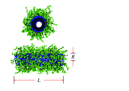
A cylindrical membrane, composed of $N_{\rm{mb}}=1200$, with $N_{\rm{chain}}$ anchored polymers outside (see Fig. 2) is used to estimate the polymer-induced spontaneous curvature and bending rigidity. For a cylindrical membrane with a radius $R$ and a length $L_{z}$, the curvature free energy is given by

$$F_{\rm{cv}} = \int\Big{[}\frac{\kappa}{2}(C_{1}+C_{2}-C_{0})^{2}+\bar{\kappa}C_{1}C_{2}\Big{]}dA$$ (17)

$$= 2\pi RL_{z}\left[\frac{\kappa}{2}\left(\frac{1}{R}-C_{0}\right)^{2}\right],$$

where $C_{1}$ and $C_{2}$ are the principal curvatures at each position on the membrane surface, and the membrane area $A=2\pi RL_{z}$. The coefficients $\kappa$ and $\bar{\kappa}$ are the bending rigidity and saddle-splay modulus, respectively. Biomembranes with lipids symmetrically distributing in both leaflets of the bilayer have zero spontaneous curvature $C_{0}=0$. The anchored polymer outside induces asymmetry to the membrane.

The bending energy of the membrane generates a shrinking force along the cylindrical axis,

$$f_{z}=\frac{\partial F_{\rm{cv}}}{\partial L_{z}}=2\pi\kappa\Big{(}\frac{1}{R}-C_{0}\Big{)}.$$ (18)

Since a shorter cylinder membrane has a larger cylindrical radius, it has a lower bending energy. Previously, we clarified that this force can be used to estimate the spontaneous curvature $C_{0}$ and bending rigidity $\kappa$ in simulations A:Hay2011 . We calculated $C_{0}$ and $\kappa$ for another meshless model, which has an orientational degree of freedom and can have a finite $C_{0}$. The obtained values of $C_{0}$ agree very well with those calculated from an alternative method using a curved membrane strip.

Figure 4: Polymer-induced spontaneous curvature is estimated by the linear fitting method. It increases with increasing anchored polymer density.

Figure 5: Bending rigidity is estimated by the linear fitting method. It increases with increasing anchored polymer density.

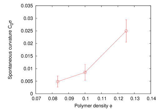
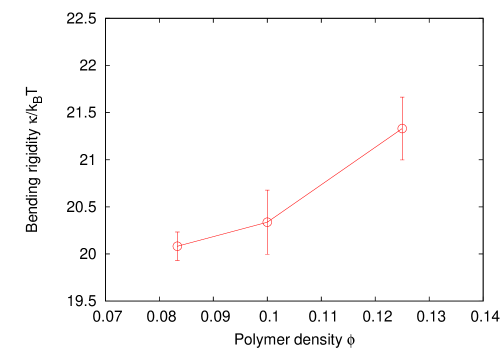
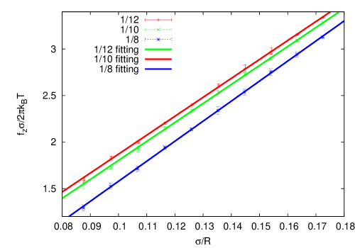
We define a polymer density $\phi=N_{\rm{chain}}/N_{\rm{mb}}$ to quantitatively describe the relation between the change of mechanical properties of membranes and the anchored polymer concentration. Figures 3 shows the axial force $f_{z}$ calculated from the pressure tensor with different polymer densities. The force $f_{z}$ increases linearly with $1/R$. Thus, $C_{0}$ and $\kappa$ of the grafted membranes can be estimated from the least squares fits to Eq. (18). The obtained values of $C_{0}$ and $\kappa$ are shown in Figs. 4 and 5, respectively. Both quantities increase with increasing anchored polymer density. This quantitatively agrees with the previous theory for a low polymer density. When the membrane is curved in the opposite direction from the polymer grafting, the polymer chains have more space to move. These entropic effects generate the spontaneous curvature of the membranes. The details of our results and comparison with the theory will be described elsewhere A:Hao2013 .

IV summary

We have studied the effects of grafted polymer on the membrane properties. Anchored polymer chains are added to a meshless membrane model. The free energy of polymer chains is dominated by the entropic effects induced by the degree of freedom of polymer conformation. We confirm that the induced spontaneous curvature and bending rigidity both increase as the polymer chain density increases. Anchored polymer chains also affect other properties of biomembranes (it will be described in Ref. A:Hao2013 ). The properties and stability of membranes can be controlled by the decoration of membrane with grafted polymers.

References

- (1) B. Alberts, A. Johnson, J. Lewis, M. Raff, K. Roberts, and P. Walter, Molecular Biology of the Cell, Garland Science, fifth edition, 2007, pp. 617–650.
- (2) E. Sackmann, “Biological Membranes Architecture and Function” in Structure and Dynamics of Membranes: I. From Cells to Vesicles, edited by R. Lipowsky, and E. Sackmann, North Holland, Amsterdam, 1995, pp. 1–65.
- (3) U. Seifert, Adv. Phys. 46, 13–137 (1997).
- (4) R. Lipowsky, Europhys. Lett. 30, 197–202 (1995).
- (5) C. Hiergeist, and R. Lipowsky, J. Phys. II France 6, 1465–1481 (1996).
- (6) T. Auth, and G. Gompper, Phys. Rev. E 68, 051801/1–6 (2003).
- (7) H.-G. Döbereiner, O. Selchow, and R. Lipowsky, Eur. Biophys. J. 28, 174–178 (1999).
- (8) R. Lipowsky, and H.-G. Döbereiner, Physica A 249, 536–543 (1998).
- (9) R. Lipowsky, and H.-G. Döbereiner, Europhys. Lett. 43, 219–225 (1998).
- (10) D. Needham, K. Hristova, T. J. McIntosh, M. Dewhirst, N. Wu, and D. D. Lasic, J Liposome Res. 2, 411–430 (1992).
- (11) C. Allen, N. Dos Santos, R. Gallagher, G. N. C. Chiu, Y. Shu, W. M. Li, S. A. Johnstone, A. S. Janoff, L. D. Mayer, M. S. Webb, and M. B. Bally Biosci. Rep. 22, 225–250 (2002).
- (12) H. Noguchi, J. Phys. Soc. Jpn. 78, 041007/1–9 (2009).
- (13) H. Noguchi, and G. Gompper, Phys. Rev. E 73, 021903/1–12 (2006).
- (14) H. Shiba, and H. Noguchi, Phys. Rev. E 84, 031926/1–13 (2011).
- (15) H. Wu, H. Shiba, and H. Noguchi, to be submitted.