Energy–momentum tensor from the Yang–Mills gradient flow

Abstract

The product of gauge fields generated by the Yang–Mills gradient flow for positive flow times does not exhibit the coincidence-point singularity and a local product is thus independent of the regularization. Such a local product can furthermore be expanded by renormalized local operators at zero flow time with finite coefficients that are governed by renormalization group equations. Using these facts, we derive a formula that relates the small flow-time behavior of certain gauge-invariant local products and the correctly-normalized conserved energy–momentum tensor in the Yang–Mills theory. Our formula provides a possible method to compute the correlation functions of a well-defined energy–momentum tensor by using lattice regularization and Monte Carlo simulation.

B01, B31, B32, B38

1 Introduction

Although lattice regularization provides a very powerful non-perturbative formulation of field theories, it is unfortunately incompatible with fundamental global symmetries quite often. The most well-known example is chiral symmetry Nielsen:1980rz ; Nielsen:1981xu ; supersymmetry is another infamous example Dondi:1976tx , as is, needless to say, translational invariance. When a regularization is not invariant under a symmetry, it is not straightforward to construct the corresponding Noether current that is conserved and generates the symmetry transformation through Ward–Takahashi (WT) relations. This makes the measurement of physical quantities related to the Noether current in a solid basis very difficult. To solve this problem, one can imagine at least three possible approaches.

The first approach is an ideal one: One finds a lattice formulation that realizes (a lattice-modified form of) the desired symmetry. If such a formulation comes to hand, the corresponding Noether current can easily be obtained by the standard Noether method. The best successful example of this sort is the lattice chiral symmetry Kaplan:1992bt ; Neuberger:1997fp ; Hasenfratz:1997ft ; Hasenfratz:1998ri ; Neuberger:1998wv ; Hasenfratz:1998jp ; Luscher:1998pqa ; Niedermayer:1998bi , which can be defined with a lattice Dirac operator that satisfies the Ginsparg–Wilson relation Ginsparg:1981bj . Although this is certainly an ideal approach, it appears that such an ideal formulation does not always come to hand, especially for spacetime symmetries (see, e.g., Ref. Kato:2008sp for a no-go theorem for supersymmetry).

The second approach is to construct the Noether current by tuning coefficients in the linear combination of operators that can mix with the Noether current under lattice symmetries. For example, for the energy–momentum tensor—the Noether current associated with the translational invariance and rotational and conformal symmetries Callan:1970ze ; Coleman:1970je —one can construct a conserved lattice energy–momentum tensor by adjusting coefficients in the linear combination of dimension $4$ operators Caracciolo:1988hc ; Caracciolo:1989pt ; the overall normalization of the energy–momentum tensor has to be fixed in some other way. Although this method is in principle sufficient when the energy–momentum tensor is in “isolation”, i.e., when the energy–momentum tensor is separated from other composite operators, as in the on-shell matrix elements, it is not obvious a priori whether one can control the ambiguity of possible higher-dimensional operators that may contribute when the energy–momentum tensor coincides with other composite operators in position space. This implies that it is not obvious whether the energy–momentum tensor constructed in the above method generates correctly-normalized translations (and rotational and conformal transformations) on operators through WT relations. (If the energy–momentum tensor generates correctly-normalized translations, it is ensured Fujikawa:1980rc (see also Sect. 7.3 of Ref. Fujikawa:2004cx ) that the trace or conformal anomaly Crewther:1972kn ; Chanowitz:1972vd is proportional to the renormalization group functions Adler:1976zt ; Nielsen:1977sy ; Collins:1976yq .)

The third possible approach is to utilize some ultraviolet (UV) finite quantity. Since such a quantity must be independent of the regularization adopted (in the limit in which the regulator is removed), there emerges a possibility that one can relate the lattice regularization and some other regularization that preserves the desired symmetry. This methodology can be found e.g. in Ref. Luscher:2004fu (see also Ref. Luscher:2010ik ), where an ultraviolet finite representation of the topological susceptibility is derived. Although the derivation of the representation itself relies on a lattice regularization that preserves the chiral symmetry Kaplan:1992bt ; Neuberger:1997fp ; Hasenfratz:1997ft ; Hasenfratz:1998ri ; Neuberger:1998wv ; Hasenfratz:1998jp ; Luscher:1998pqa ; Niedermayer:1998bi , one can use any regularization (e.g., the Wilson fermion Wilson:1975hf ) to compute the representation because it must be independent of the regularization.

In the present paper, we consider the above third approach for the energy–momentum tensor, by taking the pure Yang–Mills theory as an example. For this, we utilize the so-called Yang–Mills gradient flow (or the Wilson flow in the context of lattice gauge theory) whose usefulness in lattice gauge theory has recently been revealed Luscher:2010iy ; Luscher:2010we ; Luscher:2011bx ; Borsanyi:2012zs ; Borsanyi:2012zr ; Fodor:2012td ; Fodor:2012qh ; Fritzsch:2013je ; Luscher:2013cpa . A salient feature of the Yang–Mills gradient flow is its robust UV finiteness Luscher:2011bx . More precisely, any product of gauge fields generated by the gradient flow for a positive flow time $t$ is UV finite under standard renormalization. Such a product, moreover, does not exhibit any singularities even if some positions of gauge fields coincide. The basic mechanism for this UV finiteness is that the flow equation is a type of the diffusion equation and the evolution operator in the momentum space $\sim e^{-tk^{2}}$ acts as an UV regulator for $t>0$. This property of the gradient flow implies that the definition of a local product of gauge fields for positive flow times is independent of the regularization. In our present context, there is a hope of relating quantities obtained by the lattice regularization and the dimensional regularization with which the translational invariance is manifest.

As noted in Ref. Luscher:2011bx , on the other hand, a local product of gauge fields for a positive flow time can be expanded by renormalized local operators of the original gauge theory with finite coefficients. Those coefficients satisfy certain renormalization group equations that, combined with the dimensional analysis, provide information on the coefficients as a function of the flow time. Because of the asymptotic freedom, one can then use the perturbation theory to find the asymptotic behavior of the coefficients for small flow times.

By using the above properties of the gradient flow, one can obtain a formula that relates the small flow-time behavior of certain gauge-invariant local products and the energy–momentum tensor defined by the dimensional regularization. Since the former can be computed by using the Wilson flow with lattice regularization Luscher:2010iy ; Luscher:2010we ; Luscher:2011bx ; Borsanyi:2012zs ; Borsanyi:2012zr ; Fodor:2012td ; Fodor:2012qh ; Fritzsch:2013je ; Luscher:2013cpa and the latter is conserved and generates correctly-normalized translations on composite operators, our formula provides a possible method to compute the correlation functions of a correctly-normalized conserved energy–momentum tensor by using Monte Carlo simulation.

In the present paper, we follow the notational convention of Ref. Luscher:2011bx unless otherwise stated.

2 Yang–Mills theory and the energy–momentum tensor

2.1 The energy–momentum tensor with dimensional regularization

In the present paper, we consider the $SU(N)$ Yang–Mills theory defined in a $D$ dimensional Euclidean space. The action is given by

$$S=\frac{1}{4g_{0}^{2}}\int d^{D}x\,F_{\mu\nu}^{a}(x)F_{\mu\nu}^{a}(x),$$ (2.1)

from the Yang–Mills field strength

$$F_{\mu\nu}(x)=\partial_{\mu}A_{\nu}(x)-\partial_{\nu}A_{\mu}(x)+[A_{\mu}(x),A_{\nu}(x)].$$ (2.2)

We set

$$D=4-2\epsilon,$$ (2.3)

and then the mass dimension of the bare gauge coupling $g_{0}$ is $\epsilon$.

Assuming that the theory is regularized by the dimensional regularization (for a very nice exposition, see Ref. Collins:1984xc ), one can define the energy–momentum tensor for the system (2.1) simply by (see, e.g., Ref. Freedman:1974gs )

$$T_{\mu\nu}(x)=\frac{1}{g_{0}^{2}}\left[F_{\mu\rho}^{a}(x)F_{\nu\rho}^{a}(x)-\frac{1}{4}\delta_{\mu\nu}F_{\rho\sigma}^{a}(x)F_{\rho\sigma}^{a}(x)\right],$$ (2.4)

up to terms attributed to the gauge fixing and the Faddeev–Popov ghost fields, which are irrelevant in correlation functions of gauge-invariant operators. Note that the mass dimension of the energy–momentum tensor is $D$.

The advantage of dimensional regularization is its translational invariance. Because of this property, the energy–momentum tensor naively constructed from bare quantities, Eq. (2.4), is conserved and generates correctly-normalized translations through a WT relation,

$$\int d^{D}x\,\left\langle\partial_{\mu}T_{\mu\nu}(x)\mathcal{O}\right\rangle=-\left\langle\partial_{\nu}\mathcal{O}\right\rangle,$$ (2.5)

where it is understood that the derivative on the right-hand side is acting all positions in a gauge-invariant operator $\mathcal{O}$. Used in combination with dimensional counting and gauge invariance, this WT relation implies that the energy–momentum tensor $T_{\mu\nu}(x)$ is finite Joglekar:1975jm ; Nielsen:1977sy and thus, in the minimal subtraction (MS) scheme,

$$T_{\mu\nu}(x)-\left\langle T_{\mu\nu}(x)\right\rangle=\left\{T_{\mu\nu}\right\}_{R}(x).$$ (2.6)

The finiteness of the energy–momentum tensor (2.4) provides further useful information on the renormalization of dimension $4$ gauge-invariant operators. The gauge coupling renormalisation with dimensional regularization is defined by

$$g_{0}^{2}\equiv\mu^{2\epsilon}g^{2}Z,$$ (2.7)

where $\mu$ is the renormalization scale and $Z$ is the renormalization factor. In the MS scheme,

$$Z=1-\frac{1}{\epsilon}\left[b_{0}g^{2}+\frac{1}{2}b_{1}g^{4}+O(g^{6})\right]+O\left(\frac{1}{\epsilon^{2}}\right),$$ (2.8)

and

$$b_{0}=\frac{11N}{48\pi^{2}},\qquad b_{1}=\frac{17N^{2}}{384\pi^{4}}.$$ (2.9)

From the rotational invariance that the dimensional regularization keeps, we see that the operator-renormalization possesses the following structures:

$$F_{\mu\rho}^{a}(x)F_{\nu\rho}^{a}(x)-\left\langle F_{\mu\rho}^{a}(x)F_{\nu\rho}^{a}(x)\right\rangle$$

$$=Z_{T}\left\{F_{\mu\rho}^{a}F_{\nu\rho}^{a}\right\}_{R}(x)+Z_{M}\delta_{\mu\nu}\left\{F_{\rho\sigma}^{a}F_{\rho\sigma}^{a}\right\}_{R}(x),$$ (2.10)

and

$$F_{\rho\sigma}^{a}(x)F_{\rho\sigma}^{a}(x)-\left\langle F_{\rho\sigma}^{a}(x)F_{\rho\sigma}^{a}(x)\right\rangle=Z_{S}\left\{F_{\rho\sigma}^{a}F_{\rho\sigma}^{a}\right\}_{R}(x).$$ (2.11)

Substituting the above relations into Eqs. (2.4) and (2.6), we have

$$\left\{T_{\mu\nu}\right\}_{R}(x)$$

$$=\frac{1}{g^{2}}\mu^{-2\epsilon}Z^{-1}\biggl{[}Z_{T}\left\{F_{\mu\rho}^{a}F_{\nu\rho}^{a}\right\}_{R}(x)-\frac{1}{4}(Z_{S}-4Z_{M})\delta_{\mu\nu}\left\{F_{\rho\sigma}^{a}F_{\rho\sigma}^{a}\right\}_{R}(x)\biggr{]}.$$ (2.12)

Since the left-hand side is finite for $\epsilon\to 0$, in the MS scheme in which only pole terms are subtracted, we infer (by considering the cases, $\mu\neq\nu$ and $\mu=\nu$) that

$$Z_{T}=Z=1-b_{0}g^{2}\frac{1}{\epsilon}+O(g^{4})$$ (2.13)

and

$$Z_{S}-4Z_{M}=Z.$$ (2.14)

2.2 Implications of the trace anomaly

Another important property of the energy–momentum tensor (2.4) is the trace anomaly Adler:1976zt ; Nielsen:1977sy ; Collins:1976yq ,

$$\delta_{\mu\nu}\left\{T_{\mu\nu}\right\}_{R}(x)=-\frac{\beta}{2g^{3}}\left\{F_{\rho\sigma}^{a}F_{\rho\sigma}^{a}\right\}_{R}(x).$$ (2.15)

By Eq. (2.6), this relation is equivalent to

$$\delta_{\mu\nu}\left[T_{\mu\nu}(x)-\left\langle T_{\mu\nu}(x)\right\rangle\right] =\epsilon\frac{1}{2g_{0}^{2}}F_{\rho\sigma}^{a}(x)F_{\rho\sigma}^{a}(x)-\left\langle\epsilon\frac{1}{2g_{0}^{2}}F_{\rho\sigma}^{a}(x)F_{\rho\sigma}^{a}(x)\right\rangle$$

$$\xrightarrow{\epsilon\to 0}-\frac{\beta}{2g^{3}}\left\{F_{\rho\sigma}^{a}F_{\rho\sigma}^{a}\right\}_{R}(x).$$ (2.16)

In Eqs. (2.15) and (2.16), $\beta$ denotes the $\beta$ function for $D=4$, defined by

$$\beta\equiv\left(\mu\frac{\partial}{\partial\mu}\right)_{0}g=-\frac{1}{2}g\left(\mu\frac{\partial}{\partial\mu}\right)_{0}\ln Z,$$ (2.17)

where the subscript $0$ implies that the derivative is taken while the bare quantities are kept fixed. Equations (2.8) and (2.7) yield

$$\beta=-b_{0}g^{3}-b_{1}g^{5}+O(g^{7}).$$ (2.18)

Then, substituting Eqs. (2.12) into Eq. (2.15) and using Eqs. (2.13) and (2.14), we observe that

$$\delta_{\rho\lambda}\left\{F_{\rho\sigma}^{a}F_{\lambda\sigma}^{a}\right\}_{R}(x)=\left(1-\frac{\beta}{2g}\right)\left\{F_{\rho\sigma}^{a}F_{\rho\sigma}^{a}\right\}_{R}(x),$$ (2.19)

i.e., the contraction with the metric and the minimal subtraction, the subtraction of $1/\epsilon$ poles, do not commute; this is a peculiar but legitimate property of the dimensional regularization Collins:1984xc .

Also, substituting Eqs. (2.7) and (2.11) into Eq. (2.16), we see

$$\epsilon\frac{Z_{S}}{Z}\xrightarrow{\epsilon\to 0}-\frac{\beta}{g}.$$ (2.20)

In the MS scheme in which only pole terms are subtracted, this implies

$$Z_{S}=\left(1-\frac{\beta}{g}\frac{1}{\epsilon}\right)Z=1+O(g^{4}),$$ (2.21)

and Eq. (2.14) then shows

$$Z_{M}=-\frac{\beta}{4g}Z\frac{1}{\epsilon}=\frac{b_{0}}{4}g^{2}\frac{1}{\epsilon}+O(g^{4}).$$ (2.22)

We thus observe that all the renormalization constants in Eqs. (2.10) and (2.11), $Z_{T}$, $Z_{M}$ and $Z_{S}$, in the MS scheme can eventually be expressed by the gauge coupling renormalization constant $Z$ in Eq. (2.7).

3 Yang–Mills gradient flow and the small flow-time expansion

The Yang–Mills gradient flow defines a $D+1$ dimensional gauge potential $B(t,x)$ along a fictitious time $t$, according to the flow equation

$$\partial_{t}B_{\mu}(t,x)=D_{\nu}G_{\nu\mu}(t,x)+\alpha_{0}D_{\mu}\partial_{\nu}B_{\nu}(t,x),$$ (3.1)

where the $D+1$ dimensional field strength and the covariant derivative are defined by

$$G_{\mu\nu}(t,x)=\partial_{\mu}B_{\nu}(t,x)-\partial_{\nu}B_{\mu}(t,x)+[B_{\mu}(t,x),B_{\nu}(t,x)]$$ (3.2)

and

$$D_{\mu}=\partial_{\mu}+[B_{\mu},\cdot],$$ (3.3)

respectively. The initial condition for the flow is given by the $D$ dimensional gauge potential in the previous section:

$$B_{\mu}(t=0,x)=A_{\mu}(x).$$ (3.4)

In Eq. (3.1), the last term is introduced to suppress the evolution of the field along the direction of gauge degrees of freedom. Although this term breaks the gauge symmetry, it does not affect the evolution of any gauge-invariant operators Luscher:2010iy . Note that the mass dimension of the flow time $t$ is $-2$.

Now, from the field strength extended to the $D+1$ dimension (3.2), we define a $D+1$ dimensional analogue of the energy–momentum tensor by

$$U_{\mu\nu}(t,x)\equiv G_{\mu\rho}^{a}(t,x)G_{\nu\rho}^{a}(t,x)-\frac{1}{4}\delta_{\mu\nu}G_{\rho\sigma}^{a}(t,x)G_{\rho\sigma}^{a}(t,x).$$ (3.5)

Although this is similar in form to the original energy–momentum tensor (2.4), it is not obvious a priori how this $D+1$ dimensional object and Eq. (2.4) are related (or not). To find the relationship between them is the principal task of the present paper. We also use the density operator studied in Ref. Luscher:2010iy :

$$E(t,x)\equiv\frac{1}{4}G_{\mu\nu}^{a}(t,x)G_{\mu\nu}^{a}(t,x).$$ (3.6)

Now, as shown in Ref. Luscher:2011bx , for $t>0$, any correlation function of $B_{\mu}(t,x)$ is UV finite after standard renormalization in the $D$ dimensional Yang–Mills theory. This property holds even for any local products of $B_{\mu}(t,x)$ such as Eqs. (3.5) and (3.6). Also, for small flow times, a local product of $B_{\mu}(t,x)$ can be regarded as a local field in the $D$ dimensional sense because the flow equation (3.1) is basically the diffusion equation along the time $t$ and the diffusion length in $x$ is $\sqrt{8t}$. These properties allow us to express, as explained in Sect. 8 of Ref. Luscher:2011bx , $U_{\mu\nu}(t,x)$ and $E(t,x)$ as an asymptotic series of $D$ dimensional renormalized local operators with finite coefficients. Considering the gauge invariance and the index structure, for $D=4$, we can write

$$U_{\mu\nu}(t,x)=c_{T}(t)\left\{T_{\mu\nu}\right\}_{R}(x)+c_{S}(t)\delta_{\mu\nu}\left\{\frac{1}{4}F_{\rho\sigma}^{a}F_{\rho\sigma}^{a}\right\}_{R}(x)+O(t),$$ (3.7)

where abbreviated terms are the contributions of operators with a mass dimension higher than or equal to $6$. For Eq. (3.6), we similarly have

$$E(t,x)=\left\langle E(t,x)\right\rangle+c_{E}(t)\left\{\frac{1}{4}F_{\rho\sigma}^{a}F_{\rho\sigma}^{a}\right\}_{R}(x)+O(t).$$ (3.8)

We note that, when the renormalized gauge coupling is fixed, $U_{\mu\nu}(t,x)$ (3.5) is traceless for $D=4$,

$$\delta_{\mu\nu}U_{\mu\nu}(t,x)=2\epsilon E(t,x)\xrightarrow{\epsilon\to 0}0,$$ (3.9)

because $E(t,x)$ (3.6) is finite Luscher:2010iy and does not produce a $1/\epsilon$ singularity (this explains why there is no $c$ number expectation value term in Eq. (3.7)). Thus, considering the trace part of Eq. (3.7), we see that the coefficients $c_{T}(t)$ and $c_{S}(t)$ are not independent and are related by, for $D=4$,

$$c_{S}(t)=\frac{\beta}{2g^{3}}c_{T}(t),$$ (3.10)

because of the trace anomaly (2.15).

By eliminating the renormalized action density from Eqs. (3.7) and (3.8), we have

$$\left\{T_{\mu\nu}\right\}_{R}(x)=\frac{1}{c_{T}(t)}U_{\mu\nu}(t,x)-\frac{c_{S}(t)}{c_{T}(t)c_{E}(t)}\delta_{\mu\nu}\left[E(t,x)-\left\langle E(t,x)\right\rangle\right]+O(t).$$ (3.11)

This expression relates the energy–momentum tensor (2.6) and the short flow-time behavior of gauge-invariant local products defined by the gradient flow. Thus, once the coefficients are known, one can extract the energy–momentum tensor from the $t\to 0$ behavior of the combination on the right-hand side.

4 Renormalization group equation and the asymptotic formula

4.1 Renormalization group equation for the coefficients

We now operate

$$\left(\mu\frac{\partial}{\partial\mu}\right)_{0},$$ (4.1)

on both sides of Eq. (3.7). Since the left-hand side of Eq. (3.7), i.e., Eq. (3.5), is entirely expressed by bare quantities through the flow equation (3.1) and the initial condition (3.4), the action of (4.1) on the left-hand side identically vanishes. On the right-hand side, this vanishing must hold in each power of $t$. Thus we infer that

$$\left(\mu\frac{\partial}{\partial\mu}\right)_{0}c_{T}(t)\left\{T_{\mu\nu}\right\}_{R}(x)=0,$$ (4.2)

$$\left(\mu\frac{\partial}{\partial\mu}\right)_{0}c_{S}(t)\left\{\frac{1}{4}F_{\rho\sigma}^{a}F_{\rho\sigma}^{a}\right\}_{R}(x)=0.$$ (4.3)

For the first relation (4.2), we recall that the energy–momentum tensor is not renormalized as Eq. (2.6). Then, by expressing the operation (4.1) in terms of renormalized quantities, we have

$$\left(\mu\frac{\partial}{\partial\mu}+\beta\frac{\partial}{\partial g}\right)c_{T}(t)=0.$$ (4.4)

For Eq. (4.3), on the other hand, from Eq. (2.11),

$$\left(\mu\frac{\partial}{\partial\mu}+\beta\frac{\partial}{\partial g}+\gamma_{S}\right)c_{S}(t)=0,$$ (4.5)

where

$$\gamma_{S}\equiv-\left(\mu\frac{\partial}{\partial\mu}\right)_{0}\ln Z_{S}.$$ (4.6)

Equations (2.21), (2.7), and (2.17) yield

$$\gamma_{S}=-g^{3}\frac{d}{dg}\left(\frac{\beta}{g^{3}}\right)=2b_{1}g^{4}+O(g^{6}).$$ (4.7)

Similarly, for Eq. (3.8), we have

$$\left(\mu\frac{\partial}{\partial\mu}+\beta\frac{\partial}{\partial g}\right)\left\langle E(t,x)\right\rangle=0,$$ (4.8)

$$\left(\mu\frac{\partial}{\partial\mu}+\beta\frac{\partial}{\partial g}+\gamma_{S}\right)c_{E}(t)=0,$$ (4.9)

and thus

$$\left(\mu\frac{\partial}{\partial\mu}+\beta\frac{\partial}{\partial g}\right)\frac{c_{S}(t)}{c_{E}(t)}=0.$$ (4.10)

By the standard argument and from the fact that dimensionless quantities can depend on the renormalization scale $\mu$ only through the dimensionless combination $\sqrt{8t}\mu$, the above renormalization group equations imply that

$$c_{T}(t)(g;\mu)=c_{T}(t_{0})(\bar{g}(-\xi);\mu_{0}),$$ (4.11)

$$c_{S}(t)(g;\mu)=\exp\left[\int_{0}^{-\xi}d\xi^{\prime}\,\gamma_{S}\left(\bar{g}(\xi^{\prime})\right)\right]c_{S}(t_{0})(\bar{g}(-\xi);\mu_{0}),$$ (4.12)

$$t^{2}\left\langle E(t,x)\right\rangle(g;\mu)=t_{0}^{2}\left\langle E(t_{0},x)\right\rangle(\bar{g}(-\xi);\mu_{0}),$$ (4.13)

$$\frac{c_{S}(t)}{c_{E}(t)}(g;\mu)=\frac{c_{S}(t_{0})}{c_{E}(t_{0})}(\bar{g}(-\xi);\mu_{0}),$$ (4.14)

where the dependence on the renormalized gauge coupling and on the renormalization scale has been explicitly written. In these expressions, the running coupling $\bar{g}(\xi)$ is defined by

$$\frac{d\bar{g}(\xi)}{d\xi}=\beta\left(\bar{g}(\xi)\right),\qquad\bar{g}(0)=g,$$ (4.15)

and we introduce a variable

$$\xi\equiv\ln\frac{\sqrt{8t}\mu}{\sqrt{8t_{0}}\mu_{0}}.$$ (4.16)

In the one-loop order, the running couping (4.15) is given by

$$\bar{g}(-\xi)^{2}=\frac{1}{2b_{0}}\frac{1}{-\xi+1/(2b_{0}g^{2})}=\frac{1}{2b_{0}}\frac{1}{-\ln(\sqrt{8t}\Lambda)+\ln(\sqrt{8t_{0}}\mu_{0})},$$ (4.17)

where $\Lambda$ is the $\Lambda$ parameter in the one-loop level,

$$\Lambda=\mu e^{-1/(2b_{0}g^{2})},$$ (4.18)

and the integral appearing in Eqs. (4.12) is

$$\int_{0}^{-\xi}d\xi^{\prime}\,\gamma_{S}\left(\bar{g}(\xi^{\prime})\right)=\frac{b_{1}}{b_{0}}\left[g^{2}-\bar{g}(-\xi)^{2}\right].$$ (4.19)

In the small flow-time limit $t\to 0$, $-\xi\to+\infty$ and the running coupling $\bar{g}(-\xi)$ (4.17) becomes very small thanks to the asymptotic freedom. Thus, the right-hand sides of Eqs. (4.11)–(4.14) allow us to compute the small flow-time behavior of the coefficients by using the perturbation theory.

4.2 Lowest-order approximation and the asymptotic formula

By substituting the solution of the flow equation (3.1) (see Ref. Luscher:2011bx ) in the tree-level approximation to Eq. (3.7), we have

$$c_{T}(t)=g_{0}^{2},$$ (4.20)

simply because our energy–momentum tensor (2.4) is proportional to $1/g_{0}^{2}$. If we apply the right-hand side of Eq. (4.11) to this expression by substituting Eq. (4.17), however, it depends on $\sqrt{8t_{0}}\mu_{0}$ while the left-hand side of Eq. (4.11) does not. This shows that $c_{T}(t)$ should depend on $g^{2}$ and $\sqrt{8t}\mu$ through a particular combination as (for $D=4$)

$$c_{T}(t)=g^{2}\left\{1+2b_{0}g^{2}\left[\ln(\sqrt{8t}\mu)+c_{1}\right]+O(g^{4})\right\},$$ (4.21)

where $c_{1}$ is a constant. Similarly, since the lowest-order approximation in Eqs. (3.7) and (3.8) yields

$$c_{E}(t)=1,\qquad c_{S}(t)=-\frac{b_{0}}{2}g_{0}^{2}\mu^{-2\epsilon},$$ (4.22)

where the latter follows from Eq. (3.10), from Eq. (4.14) we have

$$\frac{c_{S}(t)}{c_{E}(t)}=-\frac{b_{0}}{2}g^{2}\left\{1+2b_{0}g^{2}\left[\ln(\sqrt{8t}\mu)+c_{2}\right]+O(g^{4})\right\},$$ (4.23)

where $c_{2}$ is another constant.

Applying Eqs. (4.11) and (4.14) to above expressions and using Eq. (4.17), we finally have the asymptotic behaviors of the coefficients in Eq. (3.11),

$$\frac{1}{c_{T}(t)}\stackrel{{\scriptstyle t\to 0+}}{{\sim}}-2b_{0}\left[\ln(\sqrt{8t}\Lambda)+c_{1}\right]$$ (4.26)

and

$$\frac{c_{S}(t)}{c_{E}(t)}\stackrel{{\scriptstyle t\to 0+}}{{\sim}}-\frac{b_{0}}{2}\frac{1}{-2b_{0}\left[\ln(\sqrt{8t}\Lambda)+c_{2}\right]},$$ (4.27)

and hence

$$\frac{c_{S}(t)}{c_{T}(t)c_{E}(t)}\stackrel{{\scriptstyle t\to 0+}}{{\sim}}-\frac{b_{0}}{2}\left[1-\frac{c_{1}-c_{2}}{-\ln(\sqrt{8t}\Lambda)}\right].$$ (4.28)

That is,

$$\left\{T_{\mu\nu}\right\}_{R}(x) \stackrel{{\scriptstyle t\to 0+}}{{\sim}}\biggl{\{}-2b_{0}\left[\ln(\sqrt{8t}\Lambda)+c_{1}\right]U_{\mu\nu}(t,x)$$

$$\qquad\qquad{}+\frac{b_{0}}{2}\left[1-\frac{c_{1}-c_{2}}{-\ln(\sqrt{8t}\Lambda)}\right]\delta_{\mu\nu}\left[E(t,x)-\left\langle E(t,x)\right\rangle\right]\biggr{\}}.$$ (4.29)

This is the relation that we were seeking: One can obtain the correctly-normalized conserved energy–momentum tensor from the small flow-time behavior of gauge-invariant products given by the Yang–Mills gradient flow. It is interesting to note that the leading $t\to 0$ behavior is completely independent of the detailed definition of the gradient flow; the structure and coefficients follow solely from the finiteness of the local products and the renormalizability of the Yang–Mills theory. The sub-leading corrections in the asymptotic form, i.e., the coefficients $c_{1}$ and $c_{2}$, depend on the detailed definition of the gradient flow; in the Appendix, we compute the constants $c_{1}$ and $c_{2}$ and we have

$$c_{1} =\ln\sqrt{\pi}+\frac{7}{22}\simeq 0.890547,$$ (4.30)

$$c_{2} =\ln\sqrt{\pi}-\frac{7}{44}+\frac{b_{1}}{2b_{0}^{2}}\simeq 0.834762.$$ (4.31)

Finally, a possible method to determine the factor $\ln(\sqrt{8t}\Lambda)$ in Eq. (4.29), i.e., the flow time $t$ in the unit of the one-loop $\Lambda$ parameter (4.18), for small flow times is to use the expectation value of the density operator, Eq. (3.6). For this quantity, by applying Eqs. (4.13) and (4.17) to the result of the one-loop calculation, Eqs. (2.28) and (2.29) of Ref. Luscher:2010iy (specialized to the pure Yang–Mills theory), we have the asymptotic form,

$$t^{2}\left\langle E(t,x)\right\rangle\stackrel{{\scriptstyle t\to 0+}}{{\sim}}\frac{3(N^{2}-1)}{128\pi^{2}}\frac{1}{-2b_{0}\left[\ln(\sqrt{8t}\Lambda)+c\right]},$$ (4.32)

where

$$c\equiv\ln(2\sqrt{\pi})+\frac{26}{33}-\frac{9}{22}\ln 3\simeq 1.60396.$$ (4.33)

One may use this asymptotic representation for $\ln(\sqrt{8t}\Lambda)$ in Eq. (4.29).

5 Conclusion

In the present paper, we have derived a formula that relates the short flow-time behavior of some gauge-invariant local products generated by the Yang–Mills gradient flow and the correctly-normalized conserved energy–momentum tensor in the Yang–Mills theory. Our main result is Eq. (4.29). The right-hand side of Eq. (4.29) can be computed by the Wilson flow in lattice gauge theory with appropriate discretizations of operators, Eqs. (3.5) and (3.6) (see, e.g., Refs. Luscher:2010iy ; Borsanyi:2012zs ). Here, the continuum limit $a\to 0$ must be taken first and then the $t\to 0$ limit is taken afterwards; otherwise our basic reasoning does not hold.

Although the formula (4.29) should be mathematically correct, the practical usefulness of Eq. (4.29) is a separate issue and has to be carefully examined numerically. Since the lattice spacing $a$ must be sufficiently smaller than the square-root of the flow time $\sqrt{8t}$ for our reasoning to work, the reliable application of Eq. (4.29) will require rather small lattice spacings. One also worries about contamination by higher-dimensional operators (i.e., the $O(t)$ terms in Eqs. (3.7) and (3.8)) and the finite-size effect which we have not taken into account in the present paper. If our strategy turns to be practically feasible, it provides a completely new method to compute correlation functions containing a well-defined energy–momentum tensor. It is clear that the present approach to the energy–momentum tensor on the lattice is not limited to the pure Yang–Mills theory although the treatment might be slightly more complicated with the presence of other fields. The application will then include the determination of the shear and bulk viscosities (see, e.g., Refs. Meyer:2007ic ; Meyer:2007dy ), the measurement of thermodynamical quantities (see Ref. Giusti:2012yj and references cited therein), the mass and the decay constant of the pseudo Nambu–Goldstone boson associated with the (approximate) dilatation invariance (see Ref. Appelquist:2010gy and references cited therein), and so on.

It is also clear that our basic idea, that operators defined with lattice regularization and in the continuum theory can be related through the gradient flow is not limited to the energy–momentum tensor. For example, it might be possible to construct an ideal chiral current or an ideal supercurrent on the lattice, from the small flow-time limit of local products. It would be interesting to pursue this idea.

Appendix A One-loop calculation of coefficient functions

For calculational convenience, we define the coefficient functions $F(t)$ and $G(t)$ by

$$G_{\mu\rho}^{a}(t,x)G_{\nu\rho}^{a}(t,x)-\left\langle G_{\mu\rho}^{a}(t,x)G_{\nu\rho}^{a}(t,x)\right\rangle$$

$$\qquad{}=F(t)\left\{F_{\mu\rho}^{a}F_{\nu\rho}^{a}\right\}_{R}(x)+G(t)\delta_{\mu\nu}\left\{F_{\rho\sigma}^{a}F_{\rho\sigma}^{a}\right\}_{R}(x)+O(t).$$ (A.1)

Equation (3.5) then becomes (for $D=4$),

$$U_{\mu\nu}(t,x) =F(t)\left[\left\{F_{\mu\rho}^{a}F_{\nu\rho}^{a}\right\}_{R}(x)-\frac{1}{4}\delta_{\mu\nu}\delta_{\rho\lambda}\left\{F_{\rho\sigma}^{a}F_{\lambda\sigma}^{a}\right\}_{R}(x)\right]+O(t)$$

$$=F(t)\left[\left\{F_{\mu\rho}^{a}F_{\nu\rho}^{a}\right\}_{R}(x)-\frac{1}{4}\delta_{\mu\nu}\left(1-\frac{\beta}{2g}\right)\left\{F_{\rho\sigma}^{a}F_{\rho\sigma}^{a}\right\}_{R}(x)\right]+O(t),$$ (A.2)

where we have used Eq. (2.19). Rewriting this in favor of the energy–momentum tensor (2.12) with Eqs. (2.13) and (2.14), we have

$$U_{\mu\nu}(t,x) =F(t)\left[\left\{F_{\mu\rho}^{a}F_{\nu\rho}^{a}\right\}_{R}(x)-\frac{1}{4}\delta_{\mu\nu}\delta_{\rho\lambda}\left\{F_{\rho\sigma}^{a}F_{\lambda\sigma}^{a}\right\}_{R}(x)\right]+O(t)$$

$$=F(t)\left[g^{2}\left\{T_{\mu\nu}\right\}_{R}(x)+\frac{\beta}{8g}\delta_{\mu\nu}\left\{F_{\rho\sigma}^{a}F_{\rho\sigma}^{a}\right\}_{R}(x)\right]+O(t).$$ (A.3)

Comparison with Eq. (3.7) then shows

$$c_{T}(t)=g^{2}F(t),\qquad c_{S}(t)=\frac{\beta}{2g}F(t).$$ (A.4)

Similarly, for Eq. (3.8),

$$E(t,x) =\left\langle E(t,x)\right\rangle+\frac{1}{4}F(t)\delta_{\rho\lambda}\left\{F_{\rho\sigma}^{a}F_{\lambda\sigma}^{a}\right\}_{R}(x)+G(t)\left\{F_{\rho\sigma}^{a}F_{\rho\sigma}^{a}\right\}_{R}(x)+O(t)$$

$$=\left[\left(1-\frac{\beta}{2g}\right)F(t)+4G(t)\right]\left\{\frac{1}{4}F_{\rho\sigma}^{a}F_{\rho\sigma}^{a}\right\}_{R}(x)+O(t),$$ (A.5)

and therefore

$$c_{E}(t)=\left(1-\frac{\beta}{2g}\right)F(t)+4G(t).$$ (A.6)

This implies, for the ratio (4.23),

$$\frac{c_{S}(t)}{c_{E}(t)} =\frac{\beta}{2g}\frac{1}{1-\frac{\beta}{2g}+4G(t)/F(t)}$$

$$=-\frac{b_{0}}{2}g^{2}\left\{1+2b_{0}g^{2}\left[-\frac{1}{4}+\frac{b_{1}}{2b_{0}^{2}}\right]-4G(t)+O(g^{4})\right\}.$$ (A.7)

To find the coefficient functions $F(t)$ and $G(t)$ in Eq. (A.1), we consider the correlation function

$$\left\langle G_{\mu\rho}^{a}(t,x)G_{\nu\rho}^{a}(t,x)A_{\kappa}^{i}(w)A_{\omega}^{j}(v)\right\rangle.$$ (A.8)

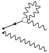
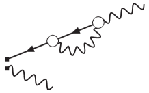
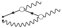
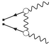
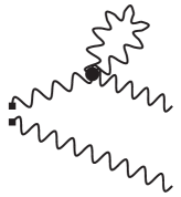
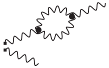
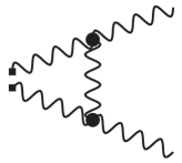
For $O(g_{0}^{2})$, there are $17$ flow-line Feynman diagrams (Figs. 1–17) that contribute to this correlation function. In the figures, gauge potentials at the flow time $t$, $B_{\mu}(t,x)$, are represented by small filled squares; the open circle denotes the flow-time vertex and the full circle is the conventional vertex in the Yang-Mills theory. We refer the reader to Ref. Luscher:2011bx for the details of the Feynman rules for flow-line diagrams.

To read off the coefficient functions $F(t)$ and $G(t)$ in Eq. (A.1) from the correlation function (A.8), we consider the vertex functions, i.e., amputated diagrams in which the external propagators of the original Yang–Mills theory are truncated. Therefore, Figs. 11, 14 and 17, which provide only the conventional wave function renormalization, should be omitted in the computation of $F(t)$ and $G(t)$. On the other hand, the flow-line propagators Luscher:2011bx , the arrowed straight lines in the diagrams, should not be truncated because these are not propagators in the quantum field theory but instead represent time evolution along the flow time.

Figure 1:

Figure 2:

Figure 3:

Figure 4:

Figure 5:

Figure 6:

Figure 7:

Figure 8:

Figure 9:

Figure 10:

Figure 11:

Figure 12:

Figure 13:

Figure 14:

Figure 15:

Figure 16:

Figure 17:

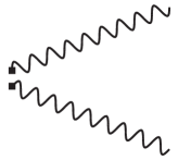
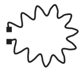
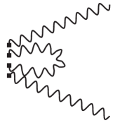
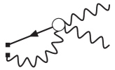
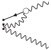
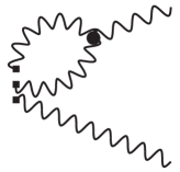
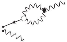
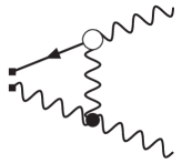
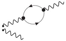
The tree-level contribution to the vertex function is

Fig. 1 $$=\delta_{\rho\sigma}\left[\int_{p,q}\,e^{i(p+q)x}\tilde{A}_{\rho}^{a}(p)\tilde{A}_{\sigma}^{a}(q)e^{-tp^{2}}e^{-tq^{2}}ip_{\mu}iq_{\nu}\pm(\mu\leftrightarrow\rho,\nu\leftrightarrow\sigma)\right]$$

$$=F_{\mu\rho}^{a}(x)F_{\nu\sigma}^{a}(x)+O(t),$$ (A.9)

where

$$A_{\mu}(x)=\int_{p}e^{ipx}\tilde{A}_{\mu}(p),\qquad\int_{p}\equiv\int\frac{d^{D}p}{(2\pi)^{D}},$$ (A.10)

and, here and in what follows, the alternating-sign symbol implies

$$t_{\mu\rho\nu\sigma}\pm(\mu\leftrightarrow\rho,\nu\leftrightarrow\sigma)\equiv t_{\mu\rho\nu\sigma}-t_{\rho\mu\nu\sigma}-t_{\mu\rho\sigma\nu}+t_{\rho\mu\sigma\nu}.$$ (A.11)

This tree-level result was used in obtaining Eq. (4.20).

The vacuum expectation value in the lowest order is

Fig. 2 $$=g_{0}^{2}\delta^{aa}\delta_{\rho\sigma}\left[\int_{\ell}\frac{1}{\ell^{2}}\,e^{-2t\ell^{2}}\ell_{\mu}\ell_{\nu}\delta_{\rho\sigma}\pm(\mu\leftrightarrow\rho,\nu\leftrightarrow\sigma)\right]$$

$$=\frac{3}{128\pi^{2}}(N^{2}-1)g_{0}^{2}\frac{1}{t^{2}}\delta_{\mu\nu}.$$ (A.12)

Now, as an example of the computation of one-loop flow-line Feynman diagrams, we briefly illustrate the computation of Fig 14. A straightforward application of the Feynman rules in Ref. Luscher:2011bx in the “Feynman gauge” in which the gauge parameters are taken as $\lambda_{0}=\alpha_{0}=1$, yields the expression,

Fig. 14 $$=Ng_{0}^{2}\delta_{\rho\sigma}\biggl{(}\int_{p,q}\,e^{i(p+q)x}\tilde{A}_{\alpha}^{b}(p)\tilde{A}_{\beta}^{c}(q)$$

$$\qquad{}\times\int_{\ell}\frac{1}{(p+\ell)^{2}}\frac{1}{\ell^{2}}\frac{1}{(q-\ell)^{2}}\,e^{-t(p+\ell)^{2}}e^{-t(q-\ell)^{2}}$$

$$\qquad\qquad{}\times i(p+\ell)_{\mu}i(q-\ell)_{\nu}$$

$$\qquad\qquad{}\times\left[\delta_{\rho\lambda}(-p-2\ell)_{\alpha}+\delta_{\lambda\alpha}(\ell-p)_{\rho}+\delta_{\alpha\rho}(2p+\ell)_{\lambda}\right]$$

$$\qquad\qquad{}\times\left[\delta_{\lambda\sigma}(-2\ell+q)_{\beta}+\delta_{\sigma\beta}(-2q+\ell)_{\lambda}+\delta_{\beta\lambda}(q+\ell)_{\sigma}\right]$$

$$\qquad\qquad\qquad{}\pm(\mu\leftrightarrow\rho,\nu\leftrightarrow\sigma)\biggr{)}.$$ (A.13)

To find the coefficients $F(t)$ and $G(t)$ in Eq. (A.1), we write this vertex function as

$$\int_{p,q}\,e^{i(p+q)x}\tilde{A}_{\alpha}^{a}(p)\tilde{A}_{\beta}^{a}(q)M_{\mu\nu,\alpha\beta}(p,q),$$ (A.14)

and find the coefficients of

$$-p_{\mu}q_{\nu}\delta_{\alpha\beta}$$ (A.15)

and

$$-4p\cdot q\delta_{\mu\nu}\delta_{\alpha\beta},$$ (A.16)

respectively, in $M_{\mu\nu,\alpha\beta}(p,q)$. For this, we first exponentiate the denominators in Eq. (A.13) by using

$$\frac{1}{(p+\ell)^{2}}\frac{1}{(q-\ell)^{2}}=\int_{0}^{\infty}d\xi\,\int_{0}^{\infty}d\eta\,e^{-\xi(p+\ell)^{2}}e^{-\eta(q-\ell)^{2}}.$$ (A.17)

We then simply expand the integrand with respect to the external momenta $p$ and $q$ to $O(p,q)$. The flow-time evolution factor $e^{-2t\ell^{2}}$ in the integrand makes the integral (A.13) UV finite for any dimension $D$. On the other hand, there always exists a complex domain of $D$ such that the integral is infrared finite; this provides the analytic continuation of the integral such that

$$\int_{\ell}\frac{1}{\ell^{2}}\,e^{-\alpha\ell^{2}}=\frac{1}{(4\pi)^{D/2}}\frac{1}{D/2-1}\alpha^{-D/2+1},$$ (A.18)

$$\int_{\ell}\frac{1}{\ell^{2}}\,e^{-\alpha\ell^{2}}\ell_{\mu}\ell_{\nu}=\frac{1}{(4\pi)^{D/2}}\frac{1}{D}\alpha^{-D/2}\delta_{\mu\nu},$$ (A.19)

$$\int_{\ell}\frac{1}{\ell^{2}}\,e^{-\alpha\ell^{2}}\ell_{\mu}\ell_{\nu}\ell_{\rho}\ell_{\sigma}=\frac{1}{(4\pi)^{D/2}}\frac{1}{2(D+2)}\alpha^{-D/2-1}\left(\delta_{\mu\nu}\delta_{\rho\sigma}+\delta_{\mu\rho}\delta_{\nu\sigma}+\delta_{\mu\sigma}\delta_{\nu\rho}\right),$$ (A.20)

$$\int_{\ell}\frac{1}{\ell^{2}}\,e^{-\alpha\ell^{2}}\ell_{\mu}\ell_{\nu}\ell_{\rho}\ell_{\sigma}\ell_{\alpha}\ell_{\beta}$$

$$=\frac{1}{(4\pi)^{D/2}}\frac{1}{4(D+4)}\alpha^{-D/2-2}\left(\delta_{\mu\nu}\delta_{\rho\sigma}\delta_{\alpha\beta}+\text{$14$ permutations}\right).$$ (A.21)

Then it is straightforward to find the coefficients of Eqs. (A.15) and (A.16), which directly make a contribution to the functions $F(t)$ and $G(t)$.

Table 1: The contributions of each flow-line Feynman diagram (in the Feynman gauge) to the coefficients of Eqs. (A.15) and (A.16), respectively, in the unit of Eq. (A.22). These correspond to the coefficient functions $F(t)$ and $G(t)$ in Eq. (A.1). The numbers with $*$ are corrected from previous versions of the present paper.

	$F(t)$	$G(t)$
Fig. 5	$0$	$0$
Fig. 5	$-3\dfrac{1}{\epsilon}-3\ln(8\pi t)-1$	$0$
Fig. 5	$-\dfrac{7}{36}$	$-\dfrac{49}{144}$
Fig. 8	$2\dfrac{1}{\epsilon}+2\ln(8\pi t)-\dfrac{1}{2}$	$0$
Fig. 8	$\dfrac{19}{288}$	$\dfrac{121}{384}$
Fig. 8	$\dfrac{35}{96}^{*}$	$\dfrac{143}{384}^{*}$
Fig. 11	$-\dfrac{25}{8}$	$0$
Fig. 11	$\dfrac{1}{3}\dfrac{1}{\epsilon}+\dfrac{1}{3}\ln(8\pi t)-\dfrac{17}{36}$	$\dfrac{7}{12}\dfrac{1}{\epsilon}+\dfrac{7}{12}\ln(8\pi t)+\dfrac{1}{144}$
Fig. 14	$-\dfrac{5}{3}\dfrac{1}{\epsilon}-\dfrac{5}{3}\ln(8\pi t)+\dfrac{25}{36}$	$-\dfrac{3}{2}\dfrac{1}{\epsilon}-\dfrac{3}{2}\ln(8\pi t)-\dfrac{29}{16}$
Fig. 14	$3\dfrac{1}{\epsilon}+3\ln(8\pi t)+3$	$0$
Fig. 17	$3\dfrac{1}{\epsilon}+3\ln(8\pi t)+\dfrac{5}{2}$	$0$
Fig. 17	$1^{*}$	$\dfrac{31}{24}$
$Z$ factors	$-\dfrac{11}{3}\dfrac{1}{\epsilon}$	$\dfrac{11}{12}\dfrac{1}{\epsilon}$

In Table 1, we summarize the contribution of each diagram computed in the above method in the unit of

$$\frac{1}{16\pi^{2}}Ng_{0}^{2}.$$ (A.22)

In the last line of the table, “$Z$ factors” implies the contributions of the one-loop operator renormalization factors, $Z_{T}$ (2.13) and $Z_{M}$ (2.22), through the tree-level diagram, Eq. (A.9) (recall Eq. (2.10)). We see that those operator renormalization factors precisely cancel the residues of $1/\epsilon$ and make the coefficients $F(t)$ and $G(t)$ finite; this is precisely what we expect from the general argument. From the results in the table, we then have

$$F(t) =1+2b_{0}g^{2}\left[\ln(\sqrt{8t}\mu)+\ln\sqrt{\pi}+\frac{7}{22}\right],$$ (A.23)

$$G(t) =-\frac{1}{2}b_{0}g^{2}\left[\ln(\sqrt{8t}\mu)+\ln\sqrt{\pi}+\frac{1}{11}\right].$$ (A.24)

Finally, comparison with the formulas (A.4), (A.7), (4.21) and (4.23) shows the results quoted in Sect. 4, Eqs. (4.30) and (4.31). Note that the coefficients of $\ln(\sqrt{8t}\mu)$ in the explicit one-loop calculation (Eqs. (A.23) and (A.24)) are in agreement with those by the general argument on the basis of the renormalization group equations and the trace anomaly (Eqs. (4.21) and (4.23)). This agreement provides a consistency check for our one-loop calculation and supports the correctness of our reasoning.

References

- (1) H. B. Nielsen and M. Ninomiya, Nucl. Phys. B 185, 20 (1981) [Erratum-ibid. B 195, 541 (1982)].
- (2) H. B. Nielsen and M. Ninomiya, Nucl. Phys. B 193, 173 (1981).
- (3) P. H. Dondi and H. Nicolai, Nuovo Cim. A 41, 1 (1977).
- (4) D. B. Kaplan, Phys. Lett. B 288, 342 (1992) [hep-lat/9206013].
- (5) H. Neuberger, Phys. Lett. B 417, 141 (1998) [hep-lat/9707022].
- (6) P. Hasenfratz, Nucl. Phys. Proc. Suppl. 63, 53 (1998) [hep-lat/9709110].
- (7) P. Hasenfratz, V. Laliena and F. Niedermayer, Phys. Lett. B 427, 125 (1998) [hep-lat/9801021].
- (8) H. Neuberger, Phys. Lett. B 427, 353 (1998) [hep-lat/9801031].
- (9) P. Hasenfratz, Nucl. Phys. B 525, 401 (1998) [hep-lat/9802007].
- (10) M. Lüscher, Phys. Lett. B 428, 342 (1998) [hep-lat/9802011].
- (11) F. Niedermayer, Nucl. Phys. Proc. Suppl. 73, 105 (1999) [hep-lat/9810026].
- (12) P. H. Ginsparg and K. G. Wilson, Phys. Rev. D 25, 2649 (1982).
- (13) M. Kato, M. Sakamoto and H. So, JHEP 0805, 057 (2008) [arXiv:0803.3121 [hep-lat]].
- (14) C. G. Callan, Jr., S. R. Coleman and R. Jackiw, Annals Phys. 59, 42 (1970).
- (15) S. R. Coleman and R. Jackiw, Annals Phys. 67, 552 (1971).
- (16) S. Caracciolo, G. Curci, P. Menotti and A. Pelissetto, Nucl. Phys. B 309, 612 (1988).
- (17) S. Caracciolo, G. Curci, P. Menotti and A. Pelissetto, Annals Phys. 197, 119 (1990).
- (18) H. Suzuki, Nucl. Phys. B 868, 459 (2013) [arXiv:1209.2473 [hep-lat]].
- (19) H. Suzuki, Phys. Lett. B 719, 435 (2013) [arXiv:1209.5155 [hep-lat]].
- (20) M. Bochicchio, L. Maiani, G. Martinelli, G. C. Rossi and M. Testa, Nucl. Phys. B 262, 331 (1985).
- (21) K. Fujikawa, Phys. Rev. D 23, 2262 (1981).
- (22) K. Fujikawa and H. Suzuki, “Path integrals and quantum anomalies,” Oxford, UK: Clarendon (2004) 284 p
- (23) R. J. Crewther, Phys. Rev. Lett. 28, 1421 (1972).
- (24) M. S. Chanowitz and J. R. Ellis, Phys. Lett. B 40, 397 (1972).
- (25) S. L. Adler, J. C. Collins and A. Duncan, Phys. Rev. D 15, 1712 (1977).
- (26) N. K. Nielsen, Nucl. Phys. B 120, 212 (1977).
- (27) J. C. Collins, A. Duncan and S. D. Joglekar, Phys. Rev. D 16, 438 (1977).
- (28) M. Lüscher, Phys. Lett. B 593, 296 (2004) [hep-th/0404034].
- (29) M. Lüscher and F. Palombi, JHEP 1009, 110 (2010) [arXiv:1008.0732 [hep-lat]].
- (30) K. G. Wilson, Subnucl. Ser. 13, 13 (1977).
- (31) M. Lüscher, JHEP 1008, 071 (2010) [arXiv:1006.4518 [hep-lat]].
- (32) M. Lüscher, PoS LATTICE 2010, 015 (2010) [arXiv:1009.5877 [hep-lat]].
- (33) M. Lüscher and P. Weisz, JHEP 1102, 051 (2011) [arXiv:1101.0963 [hep-th]].
- (34) S. Borsanyi, S. Dürr, Z. Fodor, C. Hoelbling, S. D. Katz, S. Krieg, T. Kurth and L. Lellouch et al., JHEP 1209, 010 (2012) [arXiv:1203.4469 [hep-lat]].
- (35) S. Borsanyi, S. Dürr, Z. Fodor, S. D. Katz, S. Krieg, T. Kurth, S. Mages and A. Schafer et al., arXiv:1205.0781 [hep-lat].
- (36) Z. Fodor, K. Holland, J. Kuti, D. Nogradi and C. H. Wong, JHEP 1211, 007 (2012) [arXiv:1208.1051 [hep-lat]].
- (37) Z. Fodor, K. Holland, J. Kuti, D. Nogradi and C. H. Wong, PoS LATTICE 2012, 050 (2012) [arXiv:1211.3247 [hep-lat]].
- (38) P. Fritzsch and A. Ramos, JHEP 1310, 008 (2013) [arXiv:1301.4388 [hep-lat]].
- (39) M. Lüscher, JHEP 1304, 123 (2013) [arXiv:1302.5246 [hep-lat]].
- (40) J. C. Collins, “Renormalization. An introduction to renormalization, the renormalization group, and the operator product expansion,” Cambridge, UK: Univ. Pr. (1984) 380p
- (41) D. Z. Freedman, I. J. Muzinich and E. J. Weinberg, Annals Phys. 87, 95 (1974).
- (42) S. D. Joglekar, Annals Phys. 100, 395 (1976) [Erratum-ibid. 102, 594 (1976)].
- (43) H. B. Meyer, Phys. Rev. D 76, 101701 (2007) [arXiv:0704.1801 [hep-lat]].
- (44) H. B. Meyer, Phys. Rev. Lett. 100, 162001 (2008) [arXiv:0710.3717 [hep-lat]].
- (45) L. Giusti and H. B. Meyer, JHEP 1301, 140 (2013) [arXiv:1211.6669 [hep-lat]].
- (46) T. Appelquist and Y. Bai, Phys. Rev. D 82, 071701 (2010) [arXiv:1006.4375 [hep-ph]].