An Information-Theoretic Test for Dependence
with an Application to the Temporal Structure
of Stock Returns

Abstract

Information theory provides ideas for conceptualising information and measuring relationships between objects. It has found wide application in the sciences, but economics and finance have made surprisingly little use of it. We show that time series data can usefully be studied as information – by noting the relationship between statistical redundancy and dependence, we are able to use the results of information theory to construct a test for joint dependence of random variables. The test is in the same spirit of those developed by Ryabko and Astola (2005, 2006b, 2006a), but differs from these in that we add extra randomness to the original stochatic process. It uses data compression to estimate the entropy rate of a stochastic process, which allows it to measure dependence among sets of random variables, as opposed to the existing econometric literature that uses entropy and finds itself restricted to pairwise tests of dependence. We show how serial dependence may be detected in S&P500 and PSI20 stock returns over different sample periods and frequencies. We apply the test to synthetic data to judge its ability to recover known temporal dependence structures.

Keywords: Information theory, entropy, data compression, independence test

1 Introduction

We apply some concepts from information theory to the study of time series economic phenomena. Asset pricing and statistical models of stock returns try to capture the salient features of the latent processes that generate our observed data. Information theory, following Shannon (1948), provides ideas for conceptualising information and measuring relationships between collections of objects that are highly relevant for describing the behaviour of economic time series. In finance, a time series of stock returns is a collection of real numbers that are ordered in time. The real numbers have a natural ordering, and using ideas from information theory to study the relationship between this ordering of returns and the time ordering of returns brings out salient features of the latent generating processes to be modelled.

In particular, we may ask whether there are information redundancies over time in price changes in general and stock returns in particular. Hayek (1945) argued that prices in an economy are a mechanism for communicating information that helps people to organise their behaviour, so the informativeness or uninformativeness of prices has important implications for the function or dysfunction of a capitalist system. The efficient market hypothesis (EMH) of Fama (1965) argues that asset prices reflect all available information. Since asset prices are merely summary measures of an enormous variety of market conditions, and since acting on information incurs costs to economic agents, asset prices could not possibly reflect all information, so the hypothesis is usually interpreted in terms of a normative pricing model. The EMH is an important stylisation for constructing models of macroeconomic phenomena, for making investment decisions and for assessing risk, and it has therefore been extensively tested against data. However, the EMH has proved challenging to test for at least two reasons. First, because we are faced with uncertainty about the distribution of information among economic agents and the costs they face in acting on this information. Secondly, since the hypothesis is interpreted in terms of a normative pricing model, evidence of a contradiction may be evidence against the pricing model only.

Models of asset prices are often required to show a so-called martingale property, which roughly states that betting on prices should be a fair game. Ever since Bachelier proposed a random walk model for stock prices, researchers have been interested in characterising the intertemporal dependence of the process generating returns. The independent increments property of the random walk model is known to be inconsistent with many stylised facts about stock returns: mean reversion and momentum effects, predictability of returns at daily and weekly frequencies, volatility clustering and higher volatility during U.S. market opening hours (Fama, 1991). Fama (1991) argues that predictable patterns in volatility of stock price changes are not evidence against the EMH because such predictability may be perfectly ‘rational’. General statistical dependence in the process generating stock returns is not evidence against the EMH, even though it implies that past returns can be informative about the behaviour of future returns, because there is no necessary equilibrating mechanism by which stock prices today should adjust to make our beliefs about the pattern of future returns, which are conditional on past returns, consistent with some unconditional beliefs. For example, if today’s stock prices reflect information about next year’s stock return volatility, this does not necessarily imply the existence of arbitrage. Even though statistical dependence in the process generating stock returns does not contradict the EMH, it has profound implications for the proper specification of models to describe this process.

The ideas of information redundancy and statistical dependence are strongly related, because redundant information in a sample of stock returns, for example, provides evidence for statistical dependence in the latent model that generates those returns. This is the key observation of our paper. Apart from being able to find substantial information redundancy in stock returns at various frequencies and in multiple stock markets, we are able to exploit this relationship between redundancy and dependence, which the econometrics literature has so far ignored to the best of our knowledge. Specifically we are able to offer a statistical measure of and test for dependence. This test for dependence can be applied to discover relationships in the most general sense between different random structures – even in the presence of sampling variation – and in particular can be applied to discover intertemporal dependence in stock returns. In the category of tests for dependence between real-valued random variables, including tests of serial dependence, our test has some distinct advantages over other existing methods. In general, our test can be used to discover statistical dependence in any random structures that can be represented in a computer, including text, pictures, audio and video.

Historically, measuring dependence in real-valued random variables often amounted to measuring correlation between pairs of them. However, correlation is a measure of linear association, which is only a specific type of dependence. For example, if we consider a zero-mean symmetrically distributed random variable $X$, then $X$ and $X^{2}$ have zero correlation with each other even though they are completely dependent. Over and above this problem that occurs with a pair of variables, correlation is unable to summarise the degree of dependence between more than two variables in a single number. Correlation is therefore not a sufficient or adequate measure of dependence. Many other measures of dependence with desirable properties are available in econometrics, including those based on entropy, mutual information, correlation integrals, empirical distribution functions and empirical characteristic functions. Our measure and test is most closely related to non-parametric entropy-based dependence measures of Robinson (1991), Skaug and Tjostheim (1996), Granger and Lin (1994) and Hong and White (2004). These tests measure the degree of dependence between pairs of random variables by estimating a non-parametric (kernel) joint density function, computing its entropy, and comparing this with the entropy of such a density under independence. A large difference provides evidence against the independence of these two random variables, and an asymptotic distribution theory allows one to determine if the difference is larger than one might expect as a result of sampling variation. Attractive features of entropy-based tests are that they can identify non-linear dependence (unlike correlation) and they are robust to monotonic transformations of the random variables. The main disadvantages of the existing entropy-based tests cited above are:

1. They have to be computed for pairs of random variables or pairs of lags in a time series, so they cannot measure or be used to test for joint dependence between sets of random variables. For example, they cannot test whether lags 1 to 10 of a time series contain enough of the intertemporal dependence that we may ignore other lags when specifying a model.

2. They can be sensitive to the choice of bandwidth parameter and kernel function made in density estimation. This problem is exacerbated by the fact that we need to estimate a joint distribution, rather than just a single distribution.

Our measure of and test for dependence overcomes both these problems, while preserving the advantages of an entropy measure. It is a powerful method that can test for intertemporal and cross-sectional dependence in groups of time series. In fact, the full generality of the method is remarkable.

The use of data compression in hypothesis testing is not novel. It was introduced by Ryabko and Astola (2005, 2006b, 2006a). There, the authors propose, among others, a test for serial independence that requires the computation of the so-called empirical entropy. Our approach is different in that it does not rely on the empirical entropy. In fact, our proposed test is very different and relies on computing several compression ratios. Loosely speaking, our test is as follows. Suppose you are given a sample from a stochastic process, $x_{1},...,x_{n}$, and several transformations $T_{0},T_{1},...,T_{m}$ that can be applied to that sample. Suppose additionally that, under a null hypothesis $H_{0}$ to be tested, all the transformations $T_{0}(\{X_{n}\}),T_{1}(\{X_{n}\}),...,T_{m}(\{X_{n}\})$ have the same distribution. Then, under the null hypothesis, the compression ratios of the transformations, $\rho_{0},\rho_{1},...,\rho_{m}$ should be approximately the same, and we can reject the hypothesis if they are not. In the case of our specific test all the transformations are based on random shuffles of the data, but the transformation $T_{0}$ is different from the others in that it shuffles ‘more’ the data. Then, we check whether the compression ratio corresponding to this shuffle $T_{0}$, $\rho_{0}$, is within a certain quantile of the remaining compression ratios, $\rho_{1},...,\rho_{m}$.

In the remainder of this introduction, we introduce the reader to the relevant ideas in information theory and data compression that motivate our test, and we describe the stock return data that will be used illustratively throughout. In Section 2.1, we offer a plotting procedure for visualising the degree of intertemporal structure in a single time series. In Sections 2.2 and 2.3, we apply our test of dependence to identify serial dependence in several stock return series and known stochastic processes. Section 3 concludes.

Acknowledgments

The authors wish to thank Yoel Furman for fruitul discussions and insightful comments.

1.1 Information and data compression

We can think of the information contained in a set $\mathcal{A}$ as everything in $\mathcal{A}$ that is not redundant in some sense. Compression can be achieved by finding redundancies and removing them. Data compression is the process of finding small representations of large quantities of data, where the size of the representation is usually measured in bits. Compression can be lossless, in which case the small representation is exactly equivalent to the large representation, or lossy, in which case the small representation can be made even smaller by also removing some of the most infrequently occurring data atoms. In this paper we only need to consider lossless compression.

Consider the ordered sequence of real-valued random variables $\{X_{t}:t\geq 0\}$ that we call the data generating process and suppose we have sampled finitely many realisations of this process $\{x_{t_{i}}\}=\{x_{t_{1}},x_{t_{2}},x_{t_{3}},\ldots,x_{t_{n}}\}$ for $0\leq t_{1}<t_{2}<\ldots<t_{n}$. In order to represent real numbers in a computer, we need some discretisation of the real line which defines the maximum and minimum observable real numbers and the precision of the machine. In practice, we have some discretion over this discretisation even if we are unaware of it, and finer or wider partitions can be used when the application requires it. The fineness of the partition is called the resolution of our machine, and this resolution will be relevant to our proposed test for independence. We can therefore think of the sample space of this stochastic process as being discrete. A code for this stochastic process is a bijection from the discretised real line to the set of finite sequences of bits. Given a code, the original sequence of symbols $\{x_{t_{i}}\}$ can be encoded into a sequence of bits, which we call its bit representation. The precise objective of lossless compression is to find codes with the shortest possible encoded sequences in the long run.

Example 1

Consider a stochastic process $\{X_{n}\}$ consisting of a collection of iid random variables with distribution $\mathbb{P}$ such that

$$\mathbb{P}(X=a)=\frac{1}{2},\,\,\,\mathbb{P}(X=b)=\frac{1}{4},\,\,\,\mathbb{P}(X=c)=\mathbb{P}(X=d)=\frac{1}{8}.$$

In this case, one code achieving the best possible compression rate is given by

$$a\to 0,\,\,\,b\to 10,\,\,\,c\to 110,\,\,\,d\to 111.$$

The average length of an optimally encoded sequence is, in the long run, $1.75\,\mathrm{bits}/\mathrm{symbol}$. Note that this average length coincides with the entropy rate of the stochastic process, to be defined below.

Possibly the most important quantity in information theory is the statistic known as entropy. For a discrete random variable $X_{1}$ with probability mass function $\{p_{1},p_{2},\ldots,p_{N}\}$, the entropy is defined as

$$H(X_{1})=-\sum_{i=1}^{N}p_{i}\log(p_{i}),$$

and for the unordered collection of random variables $X_{1},\ldots,X_{n}$ we can compute the entropy of the joint random variable $(X_{1},...,X_{n})$, denoted $H(X_{1},...,X_{n})$. The entropy enjoys several remarkable properties. One of these is that

$$H(X_{1},...,X_{n})\leq H(X_{1})+...+H(X_{n}),$$

with equality if and only if the random variables $X_{1},...,X_{n}$ are independent. For an overview of the remaining properties of entropy we refer the reader to Cover and Thomas (2006).

Given a stochastic process $\{X_{n}\}$, we can consider the entropy of its first $n$ random variables and study how fast this quantity grows. This leads to the definition of the entropy rate of the stochastic process $\{X_{n}\}$,

$$h(\{X_{n}\})=\lim_{n}\frac{H(X_{1},...,X_{n})}{n}.$$

whenever such a limit exists. It can be proven that for any stationary process the entropy rate is well defined, see for instance (Cover and Thomas, 2006). This entropy rate will form our measure of dependence and our test statistic. Note that for a stationary process we have the inequality

$$h(\{X_{n}\})\leq H(X_{1}),$$

or, in other words,

$$h(\{X_{n}\})=\alpha H(X_{1}),$$

for some $\alpha\in[0,1].$ In other words, the entropy rate of a stationary process can be decomposed in two components: the entropy of its marginal distribution, $H(X_{1})$, and a discount factor reflecting the intertemporal structure of the process, $\alpha$. In this work, we propose to study the intertemporal structure of returns by analising its entropy rate. For that purpose, we will need to control the contribution of the entropy of the marginal distribution to the entropy rate - we achieve this by a discretisation procedure described in detail in Section 2.1.

In the next two examples we contrast the behaviour of the entropy rate under independence and dependence. The examples use restrictive assumptions to keep the exposition as simple as possible.

Example 2

Consider a stochastic process consisting of iid random variables, $\{X_{n}\}$. Then, its entropy rate is

$$h(\{X_{n}\}) =\lim_{n}\frac{H(X_{1},...,X_{n})}{n}$$

$$=\lim_{n}\frac{\sum_{i=1}^{n}H(X_{i})}{n}$$

$$=H(X_{1}).$$

That is, in the case of an iid sequence of random variables, the entropy rate od the stochastic process coincides with the entropy rate of its marginal distribution.

Example 3

Consider a discrete one-step Markov chain with transition matrix $(P_{x_{i}x_{j}})$ for all $i,j$ and stationary distribution $\mu=(\mu_{1},...,\mu_{N})$. Let $\{X_{n}\}$ be the stochastic process obtained when we start this Markov chain from its stationary distribution. Then

$$\mathbb{P}(X_{1}=x_{1},...,X_{n}=x_{n})=\mu_{x_{1}}P_{x_{1}x_{2}}...P_{x_{n-1}x_{n}},$$

and

$$\frac{1}{n}H(X_{1},...,X_{n}) =-\frac{1}{n}\sum_{(x_{1},...,x_{n})}\mu_{x_{1}}P_{x_{1}x_{2}}...P_{x_{n-1}x_{n}}\log(\mu_{x_{1}}P_{x_{1}x_{2}}...P_{x_{n-1}x_{n}})$$

$$=\frac{H(\mu)}{n}+\frac{(n-1)}{n}\sum_{(x_{1},x_{2})}\mu_{x_{1}}P_{x_{1}x_{2}}\log(P_{x_{1}x_{2}})$$

$$\overset{n}{\underset{\infty}{\to}}\sum_{x_{1}=1}^{N}\mu_{x_{1}}H(X_{2}|X_{1}=x_{1}),$$

where $H(\mu)$ is the entropy of the stationary distribution. In other words, the entropy rate of a stationary one-step Markov chain is the average of the entropies of its $N$ conditional one-step random variables with weights given by the stationary distribution. In particular, the entropy rate of the stochastic process does not coincide with the entropy rate of its marginal distribution, it is strictly smaller..

Intuitively, the entropy rate of a stochastic process is the rate at which the number of ‘typical’ sequences grows with the length of the sequences. In other words, the number of typical sequences of length $n$ for a given stochastic process $\{X_{n}\}$ is approximately

$$2^{nh(\{X_{n}\})},$$

for $n$ sufficiently large. It is essentially because of this interpretation that, as we shall see, the entropy rate gives a sharp upper bound to the maximum lossless compression ratio of messages generated by a stochastic process. The Fundamental Theorem for a Noiseless Channel due to Shannon (1948), states that for any stationary ergodic stochastic process $\{X_{n}\}$ and for any $\varepsilon$, there exists a code with average length smaller than $h(\{X_{n}\})+\varepsilon$ bits/symbol. Furthermore, there does not exist any code with average length smaller than $h(\{X_{n}\})$ bits/symbol.

Given a stochastic process $\{X_{n}\}$, if one has access to the joint distribution of $(X_{1},...,X_{n})$, for $n$ sufficiently large, then it is possible, at least in principle, to design codes that are efficient for data generated by such a process. However, in practice there are many situations in which one does not know beforehand the distribution of the data generating process. Furthermore, even in the limited number of cases in which one does know the distribution of the data generating process, it might be unfeasible to compute the joint distribution of $(X_{1},...,X_{n})$ for $n$ large, and/or find the ‘typical’ sequences for such a distribution. Therefore, it is natural to ask whether there are universal procedures that will effectively compress any data generated by a sufficiently regular process. Our day-to-day experience with computers and celebrated tools such as zip, tells us that the answer to this question should be positive. And it is, indeed, as we shall see in the following.

There is a popular class of compression algorithms that is universally optimal and easy to implement. These are termed Lempel-Ziv, after the authors of the two basic algorithms that underlie this class, the LZ77 and LZ78. The LZ77 compression algorithm was introduced by Ziv and Lempel (1977). One year later the same authors published the LZ78 algorithm in Ziv and Lempel (1978). Loosely speaking, the Lempel-Ziv algorithms encode each sequence as a pointer to the last time that sequence occurred in the data. Because typical sequences appear more often, the pointers to the last time they occur are smaller than those for atypical sequences. One remarkable feature of these algorithms, proved by Wyner and Ziv (1991; 1994), is that they are asymptotically optimal. More precisely, given a stationary and ergodic stochastic process $\{X_{n}\}$, and denoting by $l(X_{1},...,X_{n})$ the Lempel-Ziv codeword length associated with $(X_{1},...,X_{n})$,

$$\limsup_{n}\frac{l(X_{1},...,X_{n})}{n}\leq h(\{X_{n}\}),\,\,\,a.s..$$ (1)

Since $1977$, improved implementations of Lempel-Ziv algorithms have been developed. We use one of the most recent ones, the Lempel-Ziv-Markov Algorithm (LZMA), which has been in development since $1998$ and is featured in the widely available $.7z$ compression format. Combining equation 1 with the Fundamental Theorem for a Noiseless Channel above, we can see that the average codeword length

$$\frac{l(X_{1},...,X_{n})}{n}$$

is a consistent estimator for $h(\{X_{n}\})$ when the stochastic process $\{X_{n}\}$ is stationary and ergodic. Given a computer file containing an encoding of a random sample from the stochastic process $\{X_{n}\}$, a proxy for $h(\{X_{n}\})$ is its compression ratio defined as

$$1-\frac{\mathrm{number\,of\,bits\,in\,the\,compressed\,file}}{\mathrm{number\,of\,bits\,in\,the\,uncompressed\,file}}.$$

More precisely, on the one hand, the compression ratio is an estimator of the optimal compression ratio. On the other hand, the optimal compression ratio, $\rho(\{X_{n}\})$, is related to the entropy rate via the formula

$$\rho(\{X_{n}\})=1-\frac{{h(\{X_{n}\})}}{\log(N)},$$

where $N$ is the number of possible values that the process takes. In the sequel, we will always quote compression ratios, instead of entropy rates. The reader should recall the above formula to convert between the two.

Unfortunately, to the best of our knowledge, there is currently no general result for the rate of convergence of the Lempel-Ziv algorithms to the entropy rate. To overcome this difficulty, we introduce extra randomness in the data by randomly reshuffling blocks of data. By comparing the compression rates obtained with and without the extra randomness we are able to perform inference on the entropy rate of the data-generating process. This procedure motivates the statistical test for dependence that we describe in Section 2.4.

1.2 Bias in the compression rate estimator

The skeptical reader might be wondering how ‘optimal’ these algorithms are, that is, how fast they approach optimality. We end this section with a simple experiment that ought to ‘reassure’ us that the algorithm does indeed work well. Furthermore, as we sill see, this experiment teaches us that one more factor needs to be considered before we proceed with more serious matters.

Example 4 (Convergence of the LZMA and overhead costs)

We start this example by generating a probability mass function with support in exactly $256$ points, that is a vector $p=(p_{1},...,p_{256})$ such that $\sum p_{i}=1$. This vector of probabilities is generated randomly, but with the property that the first $128$ probabilities are on average smaller than the last ones. The entropy of the resulting distribution is readily computed as $7.484616$.

The next step in this experiment is to generate $N$ i.i.d. samples in ${0,...,255}$ according to the probability mass $p$. Note that each sample can be perfectly represented using $1$ byte. Shannon’s fundamental theorem tells us, if $N$ is sufficiently large, then it should be possible to represent these $N$ samples using only $7.485$ bits, or $0.936$ bytes per sample. In other words, for $N$ sufficiently large, there exist codes that achieve a compression ratio of approximately $0.064$.

To test how the LZMA algorithm performs on this compression task we write all the $N$ samples in a binary file and compress it. Note that the size of the uncompressed file is exactly $N$ kilobytes. The result of the compression is on the following table:

	$N$	compressed size (CS)	compression ratio (CR)
1	100	222	-1.220000
2	500	621	-0.242000
3	1000	1109	-0.109000
4	5000	5003	-0.000600
5	10000	9874	0.012600
6	50000	48086	0.038280
7	100000	95598	0.044020
8	500000	475432	0.049136
9	1000000	950139	0.049861
10	5000000	4747766	0.050447
11	10000000	9495234	0.050477

Table 1: Result of compressing data generated by a source with theoretical maximum compression ratio of $0.064$.

Examining the table above generates mixed feelings. The compression ratio increases with $N$, as it should, but seems to staganate when it approaches $0.05$ which is not too close from the theoretical maximum. This leaves us wondering about where our extra compression power went, and helps us realise that there is a factor that we are not taking into account. The missing factor is overhead costs, that is, costs inherent to how the algorithm is actually implemented. These overhead costs can arise for a number of reasons, for example:

• The compressed file must carry a header with some information, which is a fixed cost.

• The LZMA needs an initial dictionary to start compressing, which might be coded in the file at a fixed cost.

Helpfully, we can estimate this overhead cost and remove it, without guessing about its origins. Consider, for that purpose, a simple experiment analogous to the previous one. First, generate a sequence of $N$ independent and identically distributed random numbers uniformly distributed in $\{0,...,255\}$. Then save the resulting sequence to a binary file and compress it using the LZMA algorithm as before. We know that this sequence is incompressible, that is its entropy $8$, the maximum possible. Therefore, the resulting “compressed” file should have the overhead costs, but no actual compression. The results of this second experiment can be found in Table 2.

	$N$	“compressed” size	overhead	overhead (%)
1	100	223	123	1.230000
2	500	631	131	0.262000
3	1000	1135	135	0.135000
4	5000	5180	180	0.036000
5	10000	10242	242	0.024200
6	50000	50831	831	0.016620
7	100000	101488	1488	0.014880
8	500000	506982	6982	0.013964
9	1000000	1013758	13758	0.013758
10	5000000	5068105	68105	0.013621
11	10000000	10135980	135980	0.013598

Table 2: Result of compressing data generated by a source with theoretical maximum compression ratio of $0$.

As we can see from this table, the overhead costs decrease with the length of our sample $N$, but is nevertheless non-negligible. These overhead costs bias our estimator of the optimal compression ration. If one takes into account these bias, we can recast the results in Table 3.

	$N$	CS	CS minus overhead	‘unbiased’ CR
1	100	222	99	0.010000
2	500	621	490	0.020000
3	1000	1109	974	0.026000
4	5000	5003	4823	0.035400
5	10000	9874	9632	0.036800
6	50000	48086	47255	0.054900
7	100000	95598	94110	0.058900
8	500000	475432	468450	0.063100
9	1000000	950139	936381	0.063619
10	5000000	4747766	4679661	0.064068
11	10000000	9495234	9359254	0.064075

Table 3: Result of compressing data generated by a source with theoretical maximum compression ratio of $0.064$ taking into account overhead costs.

Once the overhead costs are removed, we can see the compression ratio converging to the theoretical maximum. In fact, for sequences of size $5e5$ the compression ratio is already close to being optimal. Most of the datasets we will use in the sequel are smaller than this. However, the dataset of S&P500 tick data is precisely of this size. Indeed, high frequency data seems to be a good target for these techniques.

The previous example shows that our estimator of the optimal compression ratio has a bias due to overhead costs. It also shows that it is possible to remove this bias by estimating the overhead costs using an uncompressible source of data. In what follows, we will account for this bias and report only bias-corrected estimates of the compression ratios.

1.3 The stock return data

The two stock indices used in this paper are the S&P500 and the headline index of the Portuguese Stock Exchange, the PSI20. Various sample periods are used and sampling frequencies of day, minute and tick are considered. We summarise the returns series over the various samples in Table 4. All data were obtained from Bloomberg.

Table 4: Summary statistics for the return series data used in this paper.

	start	end	medianFreq
SPdaily	1928-01-03	2013-02-28	1 days
SPdaily1	1928-01-03	1949-02-10	1 days
SPdaily2	1992-12-03	2013-02-28	1 days
SPmin	2012-08-24	2013-03-01	1 mins
SPtick	2012-08-24	2013-03-01	5 secs
PSI20daily	1993-01-04	2013-02-28	1 days
PSI20min	2012-08-24	2013-03-01	1 mins
PSI20tick	2012-08-24	2013-03-01	15 secs

	0%	25%	50%	75%	100%	mean	std	skew	kurtosis
SPdaily	-0.2290	-0.004728	0.0006116	0.005506	0.1537	0.00021137	0.0120193	-0.43	18.5
SPdaily1	-0.1386	-0.007055	0.0008227	0.007590	0.1537	-0.00003762	0.0172679	0.02	8.0
SPdaily2	-0.0947	-0.004894	0.0005637	0.005848	0.1096	0.00024832	0.0120808	-0.24	8.4
SPmin	-0.0091	-0.000123	0.0000066	0.000124	0.0122	0.00000150	0.0003104	1.15	123.3
SPtick	-0.0036	-0.000020	-0.0000065	0.000020	0.0065	0.00000014	0.0000622	1.65	487.2
PSI20daily	-0.1038	-0.004769	0.0003603	0.005537	0.1020	0.00013639	0.0114057	-0.35	8.5
PSI20min	-0.0191	-0.000183	0.0000038	0.000188	0.0122	0.00000290	0.0004063	-0.88	158.7
PSI20tick	-0.0189	-0.000096	0.0000034	0.000099	0.0116	0.00000102	0.0002448	-1.92	363.5

2 Method and results

In this section, we describe our methodology and present our results. In Section 2.1, we describe how an effective discretisation of the data is useful to detect its intertemporal statistical structure. In Section 2.2, we describe how combining a bootstrapping method with compression algorithms can give insight on the dependence of random variables. In the same section, we present our findings in the returns data. In Section 2.3, we introduce the serial dependence function which measures the increase in dependence obtained from considering bigger collections of consecutive time-series points. In Section 2.4, we summarise the methodology by formalising it a statistical test. Finally, in Section 2.5, we test our methodology in synthetic data. Additionally, in the same section, we use this technique to measure the goodness of fit of a GARCH(1,1) model to S&P500 daily returns.

2.1 Visualisation of temporal dependence in quantiles at high frequencies

Consider again the sample $\{x_{t_{i}}\}=\{x_{t_{1}},x_{t_{2}},x_{t_{3}},\ldots,x_{t_{n}}\}$ for $0\leq t_{1}<t_{2}<\ldots<t_{n}$ defined in Section 1.1. We want to study the ‘structure’ of this sample to make inferences about the data generating process. The structure that we examine is the relationship between the longitudinal or time series ordering of the sample to its ordering in terms of the $\leq$ relation on $\mathbb{R}$. We could define the (longitudinal) empirical cumulative distribution function

$$\hat{F}(x)=\frac{1}{n}\sum_{i=1}^{n}\mathbb{I}\{x_{t_{i}}\leq x\},$$ (2)

and by applying the transformation $x\longmapsto n\hat{F}(x)$ to our sample, we would obtain the time-ordered ranks of the values in our sample. These ranks are detailed in that they span the integers $\{1,2,\ldots,n\}$, and for the large samples that we consider, the detail prevents us from seeing patterns in our sample that are present across time with the naked eye. Now suppose that we group the observations into $2^{8}=256$ equally-sized ‘bins’ based on their rank, using the transformation $x\longmapsto\lfloor 2^{8}\hat{F}(x)\rfloor$, where $\lfloor\cdot\rfloor$ is the usual floor function. Doing so would reduce the detail in the rank-ordering of our sample, which can be seen as a decrease in resolution or a loss of information. We would obtain from our sample a sequence of length $n$, taking values on the integers $\{1,2,3,\ldots,2^{8}\}$, and this sequence would describe the time evolution of high and low values in our sample, where ‘high’ and ‘low’ are understood in terms of the set $\{1,2,3,\ldots,2^{8}\}$ rather than the set $\{1,2,\ldots,n\}$. To enable a visualisation, we have effectively discretised the sample space $\mathbb{R}$ into $2^{8}$ regions based on the quantiles $\{2^{-8}i:i=0,1,2,\ldots,2^{8}\}$ of the distribution function $\hat{F}$. The exact partition of $\mathbb{R}$ obtained via this method is the one obtained by applying the inverse cumulative distribution function

$$\hat{F}^{-1}(q):=\inf\{x|\hat{F}(x)\leq q\}$$

to $[0,1]$. Therefore, our discretisation will have more resolution in areas where the density corresponding to $\hat{F}$ is more peaked. We could use the terminology ‘states’ to refer to the indexing set $\{1,2,3,\ldots,2^{8}\}$ and we could plot these states against time to visualise local serial dependencies in the value of our process. If the underlying data generating process were a sequence of independent (but not necessarily identically distributed) random variables, we would expect a uniformly random scatter of points across states and time. We say that this procedure performs a rank plot with 8 bits of resolution.

We apply the above method to our samples of S&P500 returns at day, minute and tick frequencies and plot the results in Figure 1. Note that each panel in Figure 1 shows only one time series, despite the discernible horizontal lines. In this rank plot with 8 bits of resolution, we can interpret the returns series as a discrete Markov chain of unknown lag order, transitioning at every point on the $x$-axis to one of $2^{8}$ possible states. From inspecting the figure, we can discern some time structure in the returns, in the form of patterns in the black and white regions of the plot, with more structure at higher frequencies. The daily returns show more time structure in the first half of the sample period than in the second half. Near the beginning of the sample period, the observations are clustered in the top and bottom states, which are the extremes of the (longitudinal) distribution of returns, and clustered away from the median returns. The presence of horizontal patterns in the first half of the daily returns sample period indicates some clustering of similar states or quantiles in small time intervals.

(a) Day

(b) Minute

(c) Tick

Figure 1: The time evolution of $256$ quantiles of returns at daily, hourly and tick frequencies.

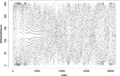
Smart algorithms for pattern detection, like data compression algorithms, can discover these patterns and others hidden from the human eye. By representing the original data equivalently as combinations of commonly-occuring patterns, these algorithms can distill a large data set into an equivalent smaller data set, and the amount by which the size of the data set is reduced is a measure of the redundancy in the original data set.

2.2 Compression ratios and testing for serial dependence

Returns in a computer are most often represented as 32- or 64-bit numbers. We standardise the amount of memory allocated to each return by representing each return using only 8 bits, which effectively applies the transformation $x\longmapsto\lfloor 2^{8}\hat{F}(x)\rfloor$ of the previous section to each return. Higher resolutions of 32 and 64 bits are also possible, and would result in higher compression ratios, without affecting the validity of the statistical test we would like to propose. We know that returns are not likely to be any number that a machine can represent as a 64-bit number. For example, we know the we will never observe a return of $2^{60}$, even though by representing numbers as doubles, we are effectively considering that possibility as well. Furthermore, the returns have a specific distribution which over time is centered and concentrated around zero. Just by exploiting this fact we can get a good compression ratio. However, this gain does not have to do with the intertemporal statistical structure of the signal, which is precisely what we propose to study. Therefore, we transform the returns in the above way so that all combinations of 8 bits appear equally often. These issues of the resolution with which to represent numbers are implicitly present also in other econometric tests of dependence.

After choosing the resolution, the various redundancies that a lossless compression algorithm can detect are

1. Time series patterns – this is the temporal dependency that we would like to isolate from the entropy rate estimator of the returns series.

2. Within-number patterns – these are inefficiencies in the machine representation of the numbers themselves and would arise, for example, if we used a 64 bit number to represent a return with mean close to zero and standard deviation $\ll 1$.

By applying our above transformation and 8-bit representation, we can eliminate much of the non-temporal relationships in our data. In other words, we control the contribution of the marginal distribution of returns to the entropy rate of the return process. Then, to study the intertemporal component of the entropy rate we perform random shuffles of blocks of data. By varying the block size used in the shuffling procedure, we can assess the contribution of the dependence within each block to the overall entropy rate of the process. Note that in the extremes of this spectrum of shuffles are the shuffles of blocks of size $1$ - which shuffles all the data and destroys all the intertemporal structure - and the shuffles of blocks of size $n$ - which does not shuffle at all and therefore does not destroy any intertemporal structure.

In Figure 2, we show the compression ratios achievable for the S&P500 and PSI returns series at frequencies of day, minute and tick for. The $y$-axis plots the unbiased estimate of the compression ratio of the underlying stochastic process computed for shuffles of blocks of varying length (ranging from $1$ to $n$, where $n$ is the length of the time-series). In each panel, the estimate of the compression ratio of the returns generating process is the vertical height at the rightmost point on the $x$-axis. A higher compression ratio indicates more statistical redundancy in the returns series, which occurs at higher frequencies and more so on the PSI than the S&P500.

(a) S&P500 Day

(b) PSI Day

(c) S&P500 Minute

(d) PSI Minute

(e) S&P500 Tick

(f) PSI Tick

Figure 2: Entropy rate estimators for original return series, and box-and-whisker plots summarising the entropy rate estimators for shuffled return series at various block sizes. Consecutive returns are resampled in blocks of the specified size (without replacement) and for each shuffled time series of returns a compression rate estimate is calculated.

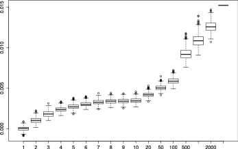
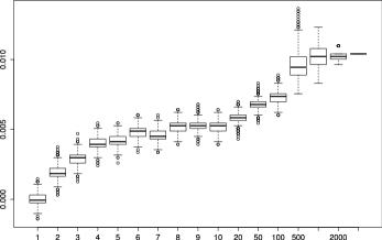
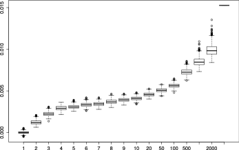
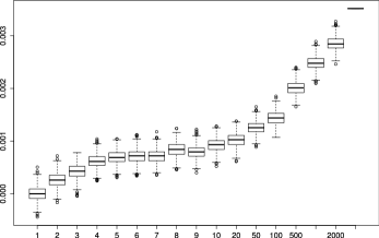
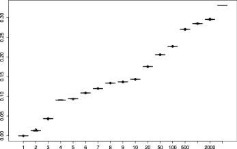
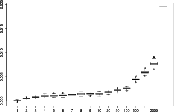
By randomly shuffling the individual returns before compressing, we are able to destroy all statistical structure/patterns in the time dimension, so that all remaining compression would come from inefficiencies in the machine representation of the numbers, less the overhead cost. Note that our 8 bit representation is very efficient so that the compressibility of the file is close to zero. The leftmost point on the $x$-axis in each panel of Figure 2 gives our compression rate estimate of an independent and identically uniform random variable, which has a mean of exactly zero and some (small) uncertainty from sampling variation. The horizontal axis in each panel shows the block size used to perform the random shuffling. For each block size we perform $1000$ shuffles so as to be able to compute confidence intervals. Returns series that have been shuffled in block sizes of 1 seem to be effectively iid and achieve a much lower compression than the original (unshuffled) returns series, which can be interpreted as saying that there is more redundancy/less statistical information in the original returns. Equivalently, the result can be interpreted as evidence for the informativeness of the time series dimension in returns data. If returns were independent (but not necessarily identically distributed) across time, their information content would not be affected by shuffling. By comparing the estimated compression ratio for the original time-series and the distribution of estimated compression rates obtained from many randomly shuffled returns, it is possible to conduct a statistical test of the independence assumption. In every panel, we see that the $p$-value of such a test would be zero, in the sense that the compression ratio from the original returns series lies above the maximum compression ratio of the returns series shuffled in blocks of size 1.

By increasing the block size, we destroy less time series structure in the original returns series, so that more compression is, on average, achievable. Equivalently, by increasing the block size, we provide more structured pseudo-return data to the compression algorithm, which tries to detect and exploit any extra information. Even at block sizes of 10 consecutive returns, we note that the compression ratio of the original return series lies above the maximum compression ratio of the shuffled return series, which means that a significant proportion of the dependence that is detectable in the original returns series is due to dependence at lags greater than 10.

As the block size grows, the compression rate estimate of the shuffled returns approaches the compression ratio for the original returns series. For any given tolerance, there is a cutoff point defined by a statistical test where the modeller is indifferent between models of lag larger than $k$ - this lag would be the one that captures, within the given tolerance, the intertemporal statistical structure of the whole series. For the block sizes shown in Figure 2, we can only identify this cutoff for the daily PSI returns. For a typical tolerance level in $[0,1/2)$, we expect the cutoff to be below lag 499, and closer to 499 than 99. In other words, for the PSI daily returns and for a tolerance level in $[0,1/2)$ a modeller will chose models with lags smaller than 499. It is then natural to consider the rate at which the mean compression ratio grows with the lag length or block size.

2.3 The lagged dependence measure and the compression ratio gap

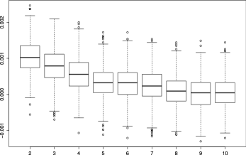
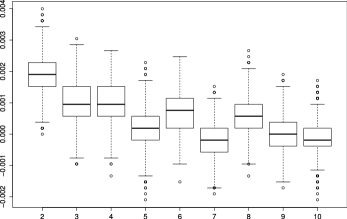
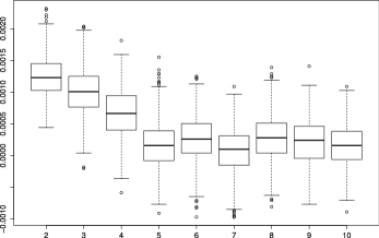
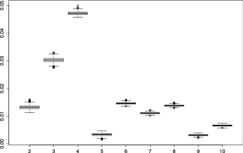
In Figure 3, we plot the increase in the estimated compression ratio between adjacent block sizes. Block sizes of lags 2 to 10 in Figure 2 therefore correspond to lags 1 to 9 in the serial dependence function of Figure 3. A point estimate for the plotted serial dependence function should be considered to be the mean of the box-and-whisker plots in Figure 3, while the spreads around the mean shown by the box-and-whisker plots are an approximation of the (100% and 75%) confidence intervals for this function. The lagged serial dependence function with its associated confidence intervals provides a natural mechanism for identifying the appropriate lag in an intertemporal model of stock returns and is a generalisation of the autocorrelation function.

Another measure that would be of interest to study in order to identify appropriate lags for modelling is the gap between compression ratios for the shuffled sequences and the compression ratio of the original squence. Contrary to the serial dependence function, these compression ratio gaps would be decreasing with increasing block size. Using this measure, a modeller would be able to find the appropriate lag for intertemporal modelling by finding the block size whose gap is within a given tolerance away from 0.

(a) S&P500 Day

(b) PSI Day

(c) S&P500 Minute

(d) PSI Minute

(e) S&P500 Tick

(f) PSI Tick

Figure 3: The serial or lagged dependence function, which is the increase in the entropy rate estimator at each lag over the entropy rate estimator at the preceding lag. Confidence intervals are approximate and are explained in Footnote 14.

2.4 A summary of the proposed test for serial dependence

For convenience, but at the cost of some redundancy(!), we summarise the steps in the test we propose for serial dependence. The test can be used for arbitrary subsets of random variables, but here we only discuss sets of consecutive returns starting at 1, in the hope that the extension is clear. These tests of dependence among subsets of random variables are highly analogous to likelihood ratio tests of sets of parameters in regression analysis, for example.

Given some sample data $\{x_{t_{1}},...,x_{t_{n}}\}$, generated by a stationary ergodic stochastic process $\{X_{n}\}$, we test the null hypothesis:

$H_{0}:$ for a given $1<k\leq n$, ${X_{1},...,X_{k}}$ are jointly independent random variables.

Note that, choosing $k=n$, we can test for independence of $X_{1},...,X_{n}$. To test the null hypothesis, we proceed as follows:

1. Compute the empirical distribution function $\hat{F}(x)$ for the data, as defined in (2).

2. Map each sample point $x_{t_{i}}$ to its discretised version using the transformation $\tilde{x}_{t_{i}}\longmapsto\lfloor 2^{8}\hat{F}(x_{t_{i}})\rfloor$. The new collection of points constitutes approximately a sample of the process $\{\tilde{X}_{n}=\lfloor 2^{8}F(X_{n})\rfloor\}$. Note that under the null hypothesis, the random variables $(\tilde{X}_{1},...,\tilde{X}_{k})$ are independent.

   For notational convenience, we denote each block $(\tilde{X}_{ki+1},...,\tilde{X}_{k(i+1)})$ by $\tilde{Y}_{i}$, for $i=0,...,I:=\lfloor n/k\rfloor-1$.

3. Given a random permutation $\sigma$ of $k$ elements, write the sequence $\tilde{y}_{\sigma(1)},...,\tilde{y}_{\sigma(I)}$ to a binary file and compress it. Given a random permutation $\phi$ of $n$ elements, write the sequence $\tilde{x}_{t_{\phi(1)}},\ldots,\tilde{x}_{t_{\phi(n)}}$ to a binary file and compress it. Store the difference between the first and second compression ratios. Repeat this step several times to obtain a distribution of the difference in compression ratios under sampling variation. Let the empirical quantile function for this distribution be denoted $Q(\cdot)$. Note that, under the null hypothesis, the distributions of $(\tilde{Y}_{\sigma(1)},...,\tilde{Y}_{\sigma(I)})$ and $(\tilde{X}_{t_{\phi(1)}},\ldots,\tilde{X}_{t_{\phi(n)}})$ are the same. Therefore, under the null hypothesis, the distribution computed before should be concentrated around $0$.

4. Given a size for the test $\alpha\in[0,1]$, reject the null hypothesis when $0<Q(\alpha)$.

We can quickly exemplify the application of this test to the daily, minute, and tick return data of the S&P and PSI. Indeed, for $k$= 2, the distribution of the difference of compression ratios computed in step 3 is represented in the left-most point of the box-whisker plots in Figure 3. A quick analysis of these plots reveals that the independence hypothesis for consecutive returns would be rejected at all confidence levels for the tick returns of the S&P and the PSI, and for the minute returns of the S&P. Furthermore, the same hypothesis would be rejected at most confidence levels for the minute returns of the PSI and daily returns of PSI and S&P. In other words, for most confidence levels, our test rejects the hypothesis of independence between consecutive returns of the S&P and PSI for daily, minute and tick frequencies.

2.5 Further examples of identifying lagged dependence

In this section, we introduce several other examples. Some of these examples come from synthetic data and serve to corroborate the power and robustness of our test. We also include an example, where our methodology is used to assess the goodness of fit of a GARCH(1,1) model, by studying the intertemporal structure of its residuals.

2.5.1 Separate sample intervals for the S&P500 returns

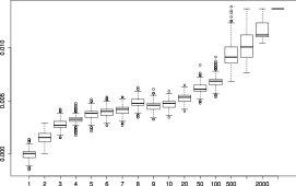
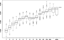
A comparison of the tests for serial dependence between the early and late samples of the S&P500, is presented in Figure 5. The plots show that S&P500 returns showed much more intertemporal structure in the early sample than in the late sample as measured by the entropy rate. The compression ratio in the early sample is estimated at about $1.1\%$, while that of the late sample is about $.7\%$. Furthermore, at minimum, about 1000 lags are required to describe the behaviour of the returns in the early sample, while about 500 may be acceptable in the late sample.

(a) Daily1 entropy rate estimators

(b) Daily2 entropy rate estimators

(c) Daily1 lagged dependence function

(d) Daily2 lagged dependence function

Figure 4: Comparing the early and late sample periods of the daily S&P500 returns series, we can see that the compression rate estimate is greater in the earlier sample.

(a) 10,000

(b) 50,000

(c) 100,000

(d) 500,000

Figure 5: Compression rate estimators against block size for the Brownian motion model of log stock prices.

2.5.2 Brownian motion model for log prices

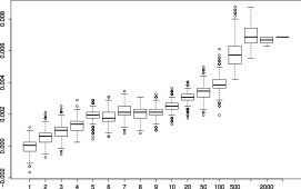
If log prices are described by a Brownian motion, then returns sampled on a uniform grid are independent and identically distributed random variables with normal distribution. We simulated one realisation of a random walk over 500,000 steps, and we show the sampling uncertainty in our estimator for various sample lengths in Figure 5. The estimates for the compression rate in the first 10, 50, 100 and 500 thousand steps are all close to zero, which is the correct quantity. The confidence intervals obtained from our shuffling procedure reliably cover the point estimator.

2.5.3 Hidden dependence in time series

We construct an artificial example of a particularly challenging stochastic process to model, and we use our method to uncover its intertemporal dependence structure. Consider the stochastic process $\{X_{n}\}$ defined on the positive integers $\mathbb{N}$ by

$$X_{n}=\begin{cases}\epsilon_{i}&n=2i-1\,\,\,\exists i\in\mathbb{N}\\ |\epsilon_{i}|\left(2\mathbb{I}\{|\epsilon_{i}|>1.19\}-1\right)&n=2i\,\,\,\exists i\in\mathbb{N}\end{cases}$$

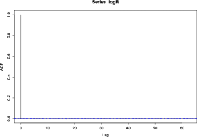
for $\epsilon_{i}\overset{iid}{{\sim}}N(0,1)\,\,\,\forall i\in\mathbb{N}$, so that the pairs $(X_{2i-1},X_{2i})$ are fully dependent, while any other pairs are not. The number $1.19$, was chosen so that the autocorrelation of the process would be approximately $0$ for all lags greater than $1$. In this case, an analysis based on use of the autocorrelation function would erroneously suggest independence. Nevertheless, our method is able to discover its dependencies. We simulate one realisation of one million observations from this process and plot the results for increasing subsamples in Figure 6. Even for the first 10,000 observations our method is able to detect significant intertemporal structure through an compression rate of $15\%$ at a $p$-value of zero. The drop in dependence at a lag length of 3 occurs because about half the odd-even pairs are broken in the shuffling of size 3 blocks, so the method is able to identify the unique pairwise dependence structure in this example. It is also interesting to notice how the compression rate approaches the optimal rate of $50\%$ as the sample size increases.

(a) 10,000

(b) 50,000

(c) 100,000

(d) 500,000

(e) 1,000,000

(f) ACF 1,000,000

Figure 6: Subfigures (a)-(e) show the compression rate estimates for the hidden dependence model at sample lengths 10, 50, 100, 500 and 1000 thousand observations. Subfigure (f) shows the autocorrelation function of the sample with length 1,000,000.

2.5.4 GARCH(1,1)

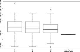
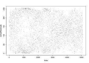
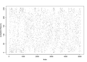
We fit a GARCH(1,1) model to the early sample (Daily1 sample) of the S&P500 returns series by maximum likelihood. In Figure 7 we see that the residuals of this model exhibit substantial dependence at all but the longest lags. By comparing this plot with Figure 5, we see that the compression rate estimates of the original returns series and the model residuals are both close to $1.1\%$. The GARCH(1,1) model therefore does not seem to remove much of the structure in returns, and the model may in fact introduce more structure than it removes. By simulating one realisation of the fitted model, we are able to recover much of its lag structure from the entropy rate estimators in panel (b). We can also see that the simulated data does not exhibit as long a memory as the original S&P500.

(a) GARCH(1,1) residuals

(b) GARCH(1,1) simulation

(c) GARCH(1,1) residuals

(d) GARCH(1,1) simulation

Figure 7: We fit a GARCH(1,1) model to the Daily1 sample of the S&P500 returns series by maximum likelihood. Subfigures (a) and (c) pertain to the residuals of this model and Subfigures (b) and (d) pertain to a single random simulation of the fitted model. (a) and (b) are the usual entropy rate estimator plots, while (c) and (d) are the rank plots at 8 bit resolution as defined in Section 2.1.

3 Conclusion

Information theory offers powerful methods that have wide applicability to the study of economic problems. Using a data compression algorithm we are able to discover substantial intertemporal dependence in stock returns in different countries, at different sampling frequencies and in different periods. We argue that this dependence does not amount to evidence against the efficient markets hypothesis, in contrast to some earlier research. We make the observation that statistical redundancy is qualitatively equivalent to evidence of dependence, and we show how to test for intertemporal dependence in time series using an estimator for entropy rate based on a data compression algorithm. By proposing a test for dependence based on the entropy rate rather than entropy, we are able to test for dependence among a group of random variables, which is an improvement over pairwise tests proposed in the literature to date. By using an asymptotically optimal compression algorithm we avoid having to estimate joint densities to estimate the entropy rate. Since general results for rates of convergence are not yet available for the compression algorithm we use, we show how a shuffling procedure can be used to nevertheless provide confidence intervals for our entropy rate estimates. We discuss how our methodology can be used in the important task of model selection, in particular to identify appropriate lags for intertemporal models. We provide strong evidence of the performance of this testing procedure under full independence and full dependence. In particular, we see how this test greatly outperforms procedures designed to detect only linear dependencies, e.g. analysis of the auto-correlation function.

In future research, we would like to refine this test, study the estimator’s rate of convergence, and provide more evidence of its performance. The potential applications of this estimator are very wide since one only requires that the objects under investigation can be stored in a computer and have a stable underlying stochastic structure.

References

- (1)
- Cover and Thomas (2006) Cover, T. M., and J. A. Thomas (2006): Elements of information theory. Wiley-interscience.
- Fama (1965) Fama, E. (1965): “The Behaviour of Stock-Market Prices,” The Journal of Business, 38(1), 34–105.
- Fama (1991) Fama, E. F. (1991): “Efficient Capital Markets: II,” The Journal of Finance, 46(5), 1575–1617.
- Granger and Lin (1994) Granger, C., and J.-L. Lin (1994): “Mutual information coefficient to identify lags in nonlinear models,” Journal of Time Series Analysis, 15(4), 371–384.
- Hayek (1945) Hayek, F. (1945): “The Use of Knowledge in Society,” The American Economic Review, 35(4), 519–530.
- Hong and White (2004) Hong, Y., and H. White (2004): “Asymptotic Distribution Theory for Nonparametric Entropy Measures of Serial Dependence,” .
- Robinson (1991) Robinson, P. (1991): “Consistent Non-Parametric Entropy-Based Testing,” Review of Economic Studies, (58), 437–453.
- Ryabko and Astola (2005) Ryabko, B., and J. Astola (2005): “Application of data compression methods to hypothesis testing for ergodic and stationary processes,” in International Conference on Analysis of Algorithms DMTCS proc. AD, vol. 399, p. 408.
- Ryabko and Astola (2006a) (2006a): “Universal codes as a basis for nonparametric testing of serial independence for time series,” Journal of Statistical Planning and Inference, 136(12), 4119–4128.
- Ryabko and Astola (2006b) (2006b): “Universal codes as a basis for time series testing,” Statistical Methodology, 3(4), 375–397.
- Shannon (1948) Shannon, C. (1948): “A Mathematical Theory of Communication,” Bell System Technical Journal, 27(July & October), 379–423 & 623–656.
- Skaug and Tjostheim (1996) Skaug, H., and D. Tjostheim (1996): “Measures of Distance Between Densities with Application to Testing for Serial Indepdence,” in Time Series Analysis in Memory of E.J. Hannan, ed. by P. Robinson, and M. Rosenblatt, pp. 363–377. Springer, New York.
- Wyner and Ziv (1991) Wyner, A., and J. Ziv (1991): “On entropy and data compression,” IEEE Trans. Inf.
- Wyner and Ziv (1994) Wyner, A., and J. Ziv (1994): “The sliding-window Lempel-Ziv algorithm is asymptotically optimal,” Proceedings of the IEEE, 82(6), 872–877.
- Ziv and Lempel (1977) Ziv, J., and A. Lempel (1977): “A universal algorithm for sequential data compression,” IEEE Trans. Information Theory, IT-23(3), 337–343.
- Ziv and Lempel (1978) (1978): “Compression of individual sequences via variable-rate coding,” IEEE Trans. Inform. Theory, 24(5), 530–536.