Turbulence Induced Collision Velocities and Rates between Different Sized Dust Grains
Abstract
We study the collision rates and velocities for point-particles of different sizes in turbulent flows. We construct fits for the collision rates at specified velocities (effectively a collisional velocity probability distribution) for particle stopping time ratios up to four; already by that point the collisional partners are very poorly correlated and so the results should be robust for even larger stopping time ratios. Significantly, we find that while particles of very different masses have approximately Maxwellian collisional statistics, as the mass ratio shrinks the distribution changes dramatically. At small stopping time ratios, the collisional partners are highly correlated and we find a population of high number density (clustered), low relative-velocity particle pairs. Unlike in the case of identical stopping time collisional partners, this low relative-velocity clustered population is collisional, but the clustering is barely adequate to trigger bulk effects such as the streaming instability. We conclude our analysis by constructing a master fit to the collisional statistics as a function only of the stopping time ratio. Together with our previous work for identical stopping time particle pairs, this provides a recipe for including collisional velocity probability distributions in dust coagulation models for protoplanetary disks. We also include our recipe for determining particle collisional diagnostics from numerical simulations.
Subject headings:
turbulence – planets and satellites: formation1. Introduction
Turbulent collisions between small dust grains is believed to lead to sticking and growth of the solids in protoplanetary disks, a crucial early step in planet formation. However, as dust grains grow in size, they respond more slowly to the gas motions. This allows two neighboring dust grains to feel the effect of larger scale, higher velocity gas motions differently, leading to higher collisional speeds. Once the particles collide with large velocities, these collisions result in growth-neutral bouncing events and, when even faster, fragmentation. While the precise speed of turbulent motions in protoplanetary disks and the material strength of the dust is unknown, the requirement that turbulence be adequately strong to explain observed accretion rates (Shakura & Sunyaev, 1973; Russell et al., 2006) imposes peak turbulent velocities noticeably above m/s, which itself is well above the dust fragmentation threshold of perhaps m/s (Blum & Wurm, 2008; Güttler et al., 2010). It follows that there is a maximum grain size beyond which equal-mass collisions will usually be too fast for the participants to survive; and so such collisions lead to fragmentation rather than further dust grain growth (Dullemond & Dominik, 2005; Zsom et al., 2010).
Historically, most of the research into turbulence induced dust-dust collisions in astrophysics was spent analytically determining a single characteristic collisional velocity scale for two dust grains of specified frictional stopping times with respect to the gas (Völk et al., 1980; Markiewicz et al., 1991; Cuzzi & Hogan, 2003; Youdin & Goodman, 2005; Ormel & Cuzzi, 2007), but there has also been significant recent numerical work (Carballido et al., 2008; Bec et al., 2010; Pan et al., 2011). Given the large turbulent velocities required to achieve significant and observed accretion flows in protoplanetary disks, this has led to the conclusion that bouncing and fragmentation barriers to collisional dust grain growth are inevitable. However, some recent work has instead focussed on the effect of including not merely a single collisional velocity scale, but rather an entire collisional velocity probability distribution (Okuzumi et al., 2011). Imposing Maxwellian distributions around the previously estimated characteristic collisional velocities, they found that small numbers of lucky grains who have multiple consecutive low-velocity encounters could grow significantly past the bouncing and even fragmentation barriers (Windmark et al., 2012; Garaud et al., 2012). This growth naturally peters out as large lucky grains are rare, and eventually unlucky collisions destroy them. However, if these lucky grains become large enough compared to the bulk population, which remains trapped by the bouncing barrier or ground up by the fragmentation barrier, then they can grow even as the result of high velocity collisions with much smaller grains in a process is referred to as mass transfer: they are large enough to survive the hits. The grain growth process then is dominated by the sweep up of small grains by a lucky few large dust grains, with equal mass collisions between the large grains being destructive but, fortunately, vanishingly rare due to their small number density.
In a previous paper (Hubbard 2012, henceforth Paper I), we looked at the collisional velocity distribution for a monodisperse population of dust grains (i.e. a population with the same gas-dust drag parameters), and found a distribution that was both lower in velocity than previously expected by a factor of approximately five, and very non-Maxwellian. Indeed, in that case the collisional velocity distribution had a pure exponentially decaying tail, and the particle pair velocity probability distribution appeared to diverge at low relative velocity. In this paper we extend that analysis to include polydisperse populations (collisions between grains of differing sizes), going from gas-dust frictional stopping time ratios of to . The stopping time scales with the grain radius and so the cube root of the mass, so our largest stopping time ratio is equivalent to a mass ratio of , large enough for mass transfer to occur. It is also large enough that we clearly approach an asymptotic limit as the two dust grains become uncorrelated.
Our goals are two-fold. Firstly, we simply wish to understand any features and behavior of the collision velocity probability distribution as there is no analytical treatment that can handle long time correlations of similar sized dust grains, and such correlations were a dominant feature in the monodisperse case. Secondly, we wish to develop a master fit for the collision velocity probability distribution as a function only of the relative size of the dust grains. Such a fit is of clear utility for any dust grain collision growth model such as used in Windmark et al. (2012) and Garaud et al. (2012). We should note that our master fit only applies in the limit of the dust grains being well contained within the turbulent cascade, as will be discussed below.
In Section 2, we discuss our turbulence model and how we extract the collisional diagnostics, going into greater detail on the latter in the appendix. In Section 3, we perform initial analysis of our results, extracting clustering information as well as the most common turbulent collisional speed. In Section 4 we examine the shapes of the collisional velocity probability distributions and create fits to them which can be used in further modeling of dust coagulation. We conclude in Section 5. In the Appendix we include a detailed procedure for extracting dust collisional diagnostics from numerical simulations.
2. Methods
As in Paper I, we evolve particles in a semi-analytic model for turbulence to extract collisional velocity probability distributions. We do this for a range of stopping time ratios, constructing fits to the collisional velocity probability distribution for each ratio, with a greater emphasis on identifying features in the distributions than pure quality of fit. Finally, we construct a fit to the fits to arrive at a final fit formula of the collisional velocity distribution with a small set of tunable parameters that can easily to used in further particle coagulation studies such as Windmark et al. (2012).
2.1. Particles
We insert particles into the synthetic turbulence field. Writing for a dust particle’s velocity and for the gas velocity at the particle’s position, the particle’s equation of motion is
| (1) |
where is the particle’s stopping time. Note that is proportional to dust grain radius for constant grain material density. All our simulations split the particles evenly between two species that differ only through their stopping times. We refer to the larger stopping time as and the smaller as . Further, we define
| (2) |
as the measure of the stopping time ratio.
The collisional properties of a dust grain pair in incompressible turbulence are expected to scale with the stopping time of the largest grain because the shorter stopping time grains are more tightly bound to the gas and particle collisions require deviations from the incompressible gas velocity. Further, dust is expected to couple (for collisional purposes) most strongly with turbulence with turnover times . This is because if the turbulence has a turnover time the dust grains will be completely entrained by the flow on a time scale and will barely deviate from the motion of the gas; while if the turbulence turnover time the dust grains will not have time to respond to the gas motion. Turbulent motions with timescales are therefore Goldilocks motions, both varying rapidly enough that the particle motion can deviate from that of the gas, and varying slowly enough that the particle motion is measurably affected.
We therefore denote and as the velocity scale and wavenumber of the turbulence with turnover time . We denote the associated velocity scale as (a dust velocity) rather than (a gas velocity) because this is the velocity scale we will use to normalize our dust collisional velocities. When is not actually included in our turbulence model (which is discrete in ), is determined by interpolating the Kolmogorov spectrum.
We consider modest due to both practical considerations (numerical resources) and because the larger case is expected to be straightforward. That is because once the stopping time ratio becomes large, the two populations of dust grains become uncorrelated, and, from the perspective of the particles with stopping time , the grains with stopping time are completely bound to the gas motion and so indistinguishable from the gas. This means that the collisional behavior will have a well defined asymptotic behavior, which we find.
Run A B C D E F G H I J K
2.2. Synthetic turbulence – Motivation
Since Kolmogorov (1941), turbulence has been understood as a cascade of kinetic energy from one lengths scale to a shorter one. The largest length scale is the one associated with the driving source of the turbulence, while the smallest length scale is determined by the viscous dissipation of the turbulent energy into heat. Between those two loosely defined scales lies the inertial range. In the inertial range the turbulence is scale free, independent of the details of the forcing and of the dissipation: the only parameter is the energy cascade rate. The Kolmogorov power spectrum of derived from the simplest dimensional analysis of the problem fits experimental data well. Significantly, in proto-planetary disks, the inertial range is believed to be large in that the ratio of the time scale associated with the largest scale motions to the time scale associated with the smallest scale motions is large: .
From the hypothesis that particle-particle collisional properties are determined by turbulence with , and the consideration of modest it follows that there are five regimes for turbulence induced particle-particle collisions, which can be describe by relating to the bounding turbulent time scales, and . The regimes are:
-
•
Particle stopping times much longer than the longest turbulent timescale, or : This regime may be accessible to direct simulation of the turbulence using Navier-Stokes with current numerical resources, although the particles will move significant distances so the numerical domains will have to be large.
-
•
Particle stopping times comparable to the longest turbulent timescale, or : This regime should be accessible to direct numerical simulation, although the applicability to protoplanetary disks may be complicated by rapid particle drift through the disk, and the results may depend sensitively on the turbulent driving mechanism.
-
•
Particle stopping times comparable to the shortest turbulent time scale, or : This regime is numerically accessible for hydrodynamical simulations, although the dissipation must be well captured.
-
•
Particle stopping times much shorter than the shortest turbulent time scale : This regime is numerically accessible.
-
•
Particle stopping times much longer than the shortest turbulent time scale, but also much shorter than the longest turbulent time scale, or : This regime is where the bouncing/fragmentation barriers are believed to lie, but is numerically inaccessible because such an inertial regime is beyond current numerical resources.
We are interested in the last regime, because full collisional velocity probability distributions are interesting precisely when collisions at different speeds have different outcomes. This regime is, however, not one that can currently be achieved through direct numerical simulation. This is our motivation for using semi-analytical synthetic turbulence: the synthetic turbulent cascade perfectly matches the Kolmogorov spectrum that fits experiment well while having a large inertial range and being numerically feasible.
2.3. Synthetic turbulence – Model
Our turbulence field uses the same approach as in Paper I: a synthetic turbulence field that matches the power spectrum of the inertial range of Kolmogorov turbulence (Kolmogorov, 1941). In other words, while the absolute scale of the kinetic energy is arbitrary, the relative energy in the motions at two given scales exactly matches that of perfect Kolmogorov turbulence, which matches experiment well.
In this model, the turbulence is binned logarithmically in wave-vector space. A region of wave-vector space with is a spherical shell, so we refer to the bins as such, and the shell is associated with . Each shell is assigned a trio of wave-vectors of the appropriate magnitude. The gas velocity associated with each wave-vector is along a velocity unit vector , so that the final velocity field is incompressible.
In Paper I we used multiple methods for introducing time variation in the velocity field, including rotating the projection of the energy in shell onto the trio of wave-vectors and varying the phase factor. In this paper, we will use the rotation of the projection, along with a slow variation in phase. The rotation of the projection occurs as a random walk of length over an eddy turnover time , and allows the velocity at a specific position to rotate in space, avoiding steady velocity patterns. The phase variation takes the form of a random walk of the phase of length over eddy turnover times. The final gas velocity field is
| (3) |
where is the velocity associated with the shell and is a unit vector that rotates as a random walk over the turbulent time scale . We set in code units. We refer the reader to Paper I for a more complete description and derivation. We will discuss the need for the phase variation in Section 2.5.
In Paper I, we found that the relative particle/gas motion in our model had reasonable statistics compared to predictions (note that particle/gas statistics are not yet well constrained as observed clustering immediately implies non-trivial particle/gas correlations, Pan et al. 2011); we also found that the particles were transported away from their positions according to a random walk, appropriate for turbulent particle diffusion. In this work, we also find in Section 3.1 that the relative motion of particles with large stopping time ratios do approach naive expectations of uncorrelated motion.
In all simulations in this paper, we include shells with ranging from to ( extending from through ). The smallest wavenumber, , corresponds to our box scale . We set and in code units, where here and refer to the largest and smallest eddy scales included in the simulation, or . Extending the Kolmogorov spectrum then, there is a value associated with any such that , although that value generally does not fall on one of the values associated with our discrete shells. In those cases we simply extrapolate the Kolmogorov spectrum. The large value of allows us to fit a particle pair with stopping time ratio of while maintaining at least . Our particle pairs are then contained within the effective turbulent cascade. We list our stopping time choices in Table 1.
2.4. Dust snap-shots
Our particles are initialized with a random position and zero velocity. In Paper I, we found that it took a significant time for the particle collisional diagnostics to achieve a steady state, in part due to the formation of dense clusters of highly correlated particles. Following that result, we take snap-shots every turbulent turnover time for the largest eddy, starting at the th turnover. We then average over the snap-shots, identifying small separation particle pairs and binning them in relative velocity (bin width ).
For a detailed description of our procedure for extracting dust collisional diagnostics from this data, see the appendix. In brief, we use the binned data to determine , which is the number of particle pairs with separation , and relative velocity . The parameter represents whether the particles have (), () or (). Note that the largest we consider is with . Comparing with the minimum velocity limit from the appendix, we note that the minimum relative velocity we can consider is
| (4) |
Our analysis remains are safely above this floor.
From we derive the fractional density enhancement over background
| (5) |
where is the number of particles, is the box volume and we treat as a smooth function. For both and , a dropped implies that we are considering only collisions between particles of differing stopping times () while a dropped implies summation over all velocity bins () or integration over velocity (). A value of is consistent with randomly distributed particles while a value of implies clustering on lengthscales of or less.
As discussed in Paper I, astrophysical particles are generally point particles in that their size is much smaller than that of relevant gas dynamical length scales. Accordingly, we will attempt to determine the limit
| (6) |
The importance of this step can be understood through a consideration of the “cold” population found in Paper I. This population was large (it dominated the particle pair counts) but interacted with itself only with velocity . The net result was that the cold population interacted at such low velocities that it provided no actual collisions despite representing the bulk of the particle pairs.
As long as both particles are well trapped within the inertial range of the turbulence, then the problem becomes scale free because the particles are too small to interact with the driving scale of the turbulence and too large to interact with the dissipative scale. It follows that all dust collisional parameters, once scaled to , must be constructible from , and knowledge of the power law of the turbulent cascade. This means that , for our fixed turbulent cascade, should be independent of the precise values of so long as they are both smaller than and and is normalized to .
2.5. Scale free behavior
As we have emphasized above, a crucial aspect of being well contained within the scale free inertial range of the turbulence is that the particle-particle collision velocity probability distribution must be scale free. Here we use the data to verify that our method produces scale free results.
Turbulent velocity fields with correlation length are expected to be uncorrelated on lengthscales . However, Equation (3) has infinite correlation lengths, which might be expected to set up undesirable correlations between particles, which we do in fact find. In Figure 1, which uses data from both Run K and an equivalent run with the time-variation of the phase turned off, we show for (black/solid and red/dashed) and for (blue/dotted and green/dash-dotted). The black/solid and blue/dotted curves do not include the time-varying phase. The -axis is plotted in units of for the particle pair, which is the gas velocity associated with turbulence with turnover time equal to the particle stopping time, different for . This means that the velocity scaling factor for any given particle pair is the one appropriate to that pair. Run K was chosen for illustrative purposes as it uses the largest and smallest values for , .
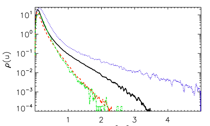
The size of , chosen to guarantee a reasonable number of pair counts at large relative velocity, is too large to derive any actual diagnostic values from the curves plotted, but a clear difficulty emerges. When the phase variation is turned off, a strong high velocity tail emerges, which is not scale free (i.e. does not scale with , the turbulent velocity scale that the particles interact with) as is shown by the distinct slopes for the two particle populations . In practice, the tail appears to be controlled by the largest scale turbulence included in the system. We attribute this problem to the infinite correlation length scale of Equation (3) which allows particle motion to be correlated over long distances if the stopping time ratio is close enough to , while physical turbulence has well defined and finite correlation lengths. When we consider polydisperse cases without time-varying phase, the effect remains noticeable for , but larger stopping time ratios break the correlations.
We break this correlation for all by adding the slow phase variation in Equation (3). While mutually approaching particles do sample the same infinite correlation length gas velocity field, the nodes () that the two particles see will be in different locations as they cross positions of the same value at different time, with different phases . In Figure 1 we see that with the phase variation turned on, the particle pair distribution reverts to being scale free as required by the turbulent cascade.
This behavior was not seen in Paper I even though there were setups where it should have occurred. This is due to Paper I’s low velocity bin cutoff and focus on small separations. At a given relative velocity , a particle pair can only close a distance of order . At low relative velocities (, the case in Paper I), particles can only close separations smaller than the appropriate turbulent length scales, so the turbulent field we used was appropriate.
3. Existence of limits
Dust grains in protoplanetary disks, generally less than centimeters in size, are much smaller than the smallest scale turbulent motions expected, which are larger than kilometer scales. Accordingly, actual collisions between such dust grains cannot be resolved in a numerical simulation. As explained in Section 2.4, we therefore take the limit for our diagnostic quantities. For finite (unlike the case!), this limit shows well defined and finite behavior for both the most common relative velocity and the total number of particle pairs.
3.1. Peak collisional velocity
In Paper I, we found that the location of the peak of in velocity space, for particles with the same stopping time, is linear in , with a intercept of . This implies the bulk of the particle population has a velocity distribution that is differentiable in space (i.e. collisionless). Allowing for different stopping times produces a different result, as shown in Figure 2, where the location of the peak remains finite even in the limit . For stopping time ratios close to , the location of the peak (at ) is approximately linear in , while it levels out for large , as seen in the lower panel of Figure 2. This is expected as in that limit, much of the relative velocity comes from the relative velocity between the larger dust grains and the gas (to which the smaller grains are tightly bound).
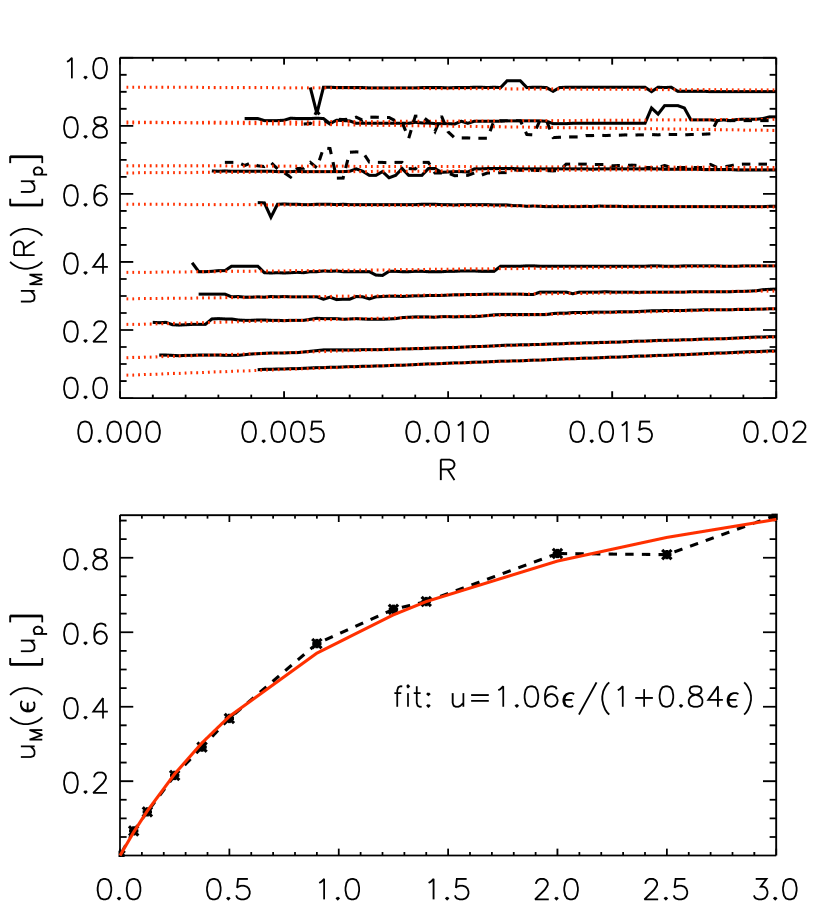
The fit in the bottom panel of Figure 2 implies a value of in the limit . While we have not yet considered the full probability distribution of the collisional velocities, this is of the same order as found analytically for this case; which is the limit for which theory should be most applicable as the long-time correlations are the weakest. In particular, Ormel & Cuzzi (2007) predict that the RMS-averaged collisional velocity should reach in this limit, which is comparable to our limit for . We can also expect from Figure 2 that collisions will be significantly slower than this value for . As particle mass scales with , this corresponds to an already noteworthy mass ratio . One of the greatest difficulties in growing particles collisionally is the fragmentation barrier, which is mitigated if the larger grain is larger enough to survive bombardment. While the collisional velocity we find is lower than that previously anticipated for , it is still high enough to lead to fragmentation for the largest scale turbulence expected in protoplanetary disks. Easing the collision velocity between near-equal mass grains should however lead to a larger production of “lucky” grains.
3.2. Clustering
Turbulence has long been known to expel heavy (higher density than the fluid) particles from high vorticity regions through centrifugal forces and concentrate them in the high strain regions between vortices (Maxey, 1987; Fessler et al., 1994; Cuzzi et al., 2001; Toschi & Bodenschatz, 2009; Pan et al., 2011). Indeed, particles with identical stopping time are strongly clustered in that the dust grain density perceived by a test grain diverges to infinity as that grain considers ever smaller spheres around itself (Pan et al. 2011, Paper I). If such clustering persists for large ranges in the stopping time ratio, the streaming instability or gravitational collapse could be triggered (Goldreich & Ward, 1973; Johansen et al., 2006, 2007; Shi & Chiang, 2013). We should note here that the vortices we consider are too small to feel any Coriolis forces that exist in a protoplanetary accretion disk. Large anti-cyclonic vortices in accretion disks are known to concentrate particles through orbital interactions(Barge & Sommeria, 1995; Johansen et al., 2004), but such effects require both rotation (which we do not include) and large enough length scales for orbital dynamics to play a major role (which we do not consider).
In Figure 3 we show the clustering, i.e. , as a function of and . In the case where , it has been found to behave as a power-law in with an exponent (Pan et al., 2011). Unlike that case, the density is not a power-law in when , instead having a well defined limit as . Further, the clustering decreases as increases, as would be expected: the position of particles with significantly different stopping times are less correlated than those of particles with similar stopping times.
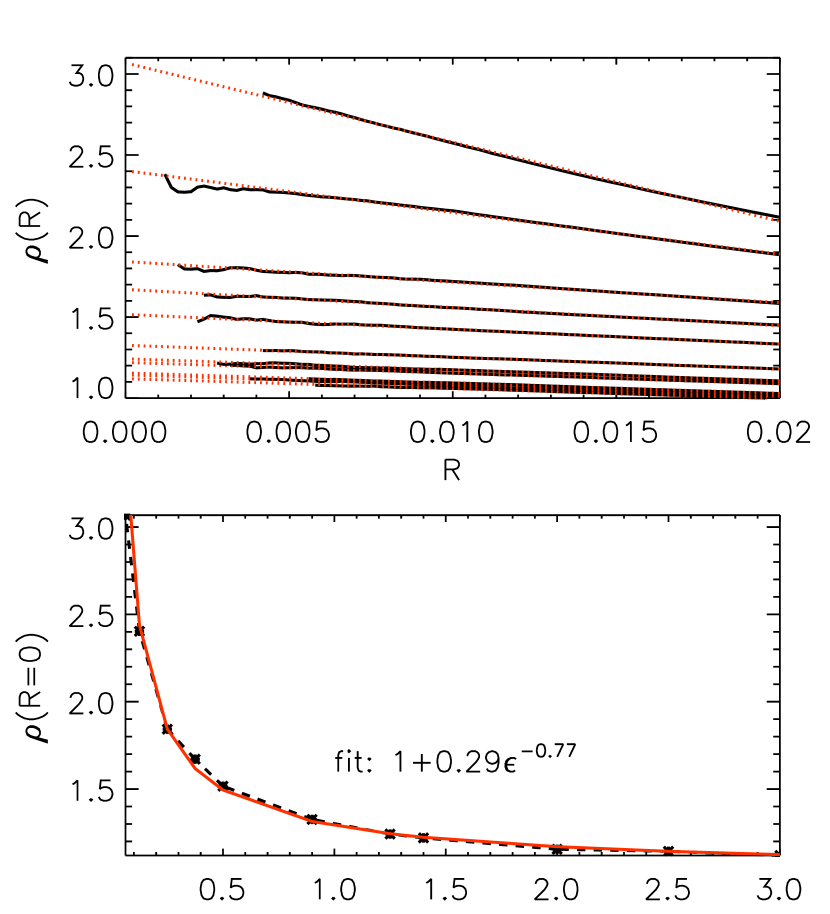
From Figure 3 it is clear that the clustering diverges as , as has been previously found for . However, because the clustering scales more weakly than it is also clear, when combining that result with Figure 2, that a net collision rate estimate does not diverge as , which was also found in Paper I. Nonetheless, the confirmation of particle clustering even for different (but similar) stopping times continues to motivate the consideration of physics relevant to mostly-collisionless clusters of dust grains, which could otherwise have been dismissed as a result specific to the monodisperse case.
It should be noted that the relatively weak power-law dependency on for the clustering implies that the extreme levels of clustering predicted will not generate high dust-to-gas mass ratio clumps. For there to be significant direct back-reaction of the dust on the gas flow, the dust-to-gas mass ratio needs to be near unity. If the volume averaged dust-to-gas ratio is the canonical this implies a –fold local increase in the dust density. To get a density enhancement over background of through turbulent clustering, we estimate a maximum range of , or , or a maximum mass ratio of . As long as the dust is not tightly concentrated at a specific grain size, the enhancement to the dust-to-gas mass ratio from turbulent clustering will be well below , and we do not have any reason to expect turbulent concentration to directly alter the character of the turbulence, meaning that our application of synthetic turbulence with no back-reaction possible is not immediately self-inconsistent. The streaming instability becomes significant for dust-to-gas mass ratios of about (Johansen et al., 2009), double the canonical disk-averaged value. This would be expected for , or a maximum mass ratio of . Triggering the streaming instability through turbulent concentration may therefore be possible, but it will require almost all the dust being found in grains of very nearly the same size.
4. Velocity distribution fit
It is now well known that the outcome of a collision between two dust grains can depend on the velocity of the collision (Güttler et al., 2010). This means that studies of collisional dust growth in protoplanetary disks need to include estimates of the rates and collisional velocity probabilities, a step recently begun by Windmark et al. (2012) and Garaud et al. (2012). However, those studies assumed Maxwellian collisional velocity distributions, which is appropriate only for uncorrelated motion. The clustering data of Figure 3 immediately implies that for modest , a Maxwellian fit is inappropriate.
In Figure 4, top panel, we show the normalized particle pair densities as a function of for our runs. While is not a constant, and so we are not correctly normalizing our lengthscales to recover perfectly scale free behavior, we can nonetheless see a change in behavior as the stopping time ratio increases, going from a sharply peaked distribution around a relatively low velocity to a much broader distribution around a significantly higher peak. We also have a qualitative change in the behavior of the high velocity tails, and the existence or non-existence of a low velocity bulge, which occurs between and . Already by the high velocity tail appears to converge.
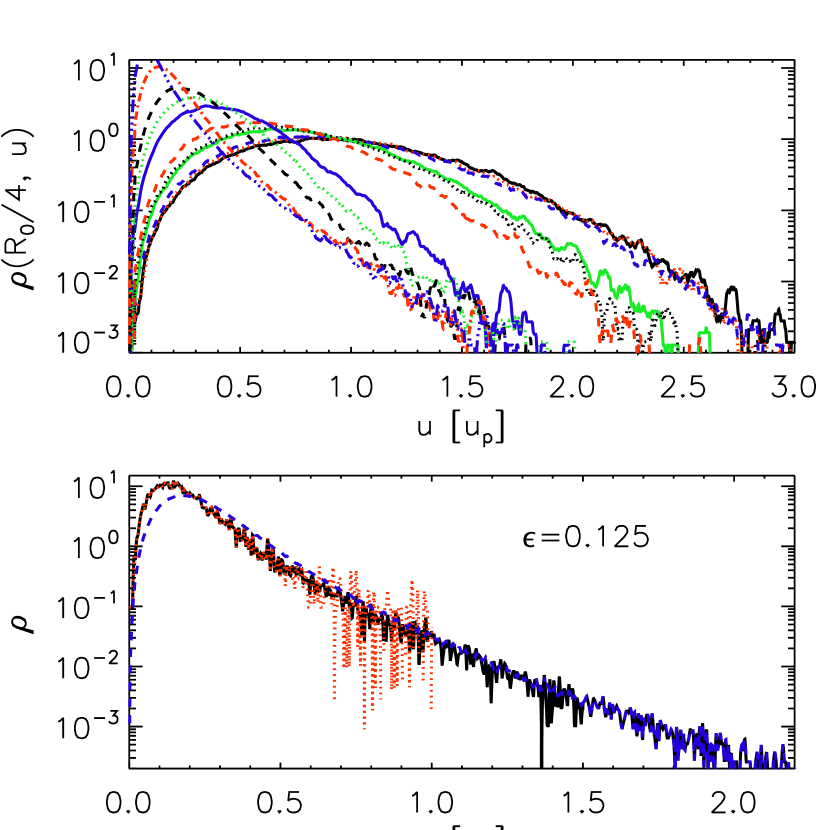
As alluded to in Section 2.5, if a particle pair has relative velocity , then they can close a distance . This means that the requirement of taking limits as is less stringent for higher relative velocities. We illustrate this in the bottom panel of Figure 4, where we show results from Run B for and , along with
| (7) |
This choice allows us to match the need for small for low relative velocities while maximizing the particle pair count for rare, high velocity pairs and avoiding sharp discontinuities. In what follows we always refer to .
4.1. Limiting cases
Before attempting to fit the entire distribution for all our stopping time ratios with a universal fit formula, we first consider subsections of the distribution.
4.1.1 Low relative velocity limit
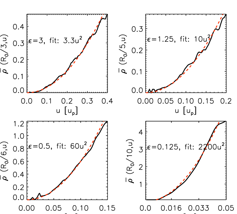
In the limit of low relative velocity , we find that for both large and small , as shown in Figure 5. This growth is faster for smaller , which is reasonable as those particle pairs are more tightly correlated, and will collide at lower velocities. Note that the increased clustering for small both allows us and requires us to consider smaller values of than for large .
4.1.2 Large – Maxwellian
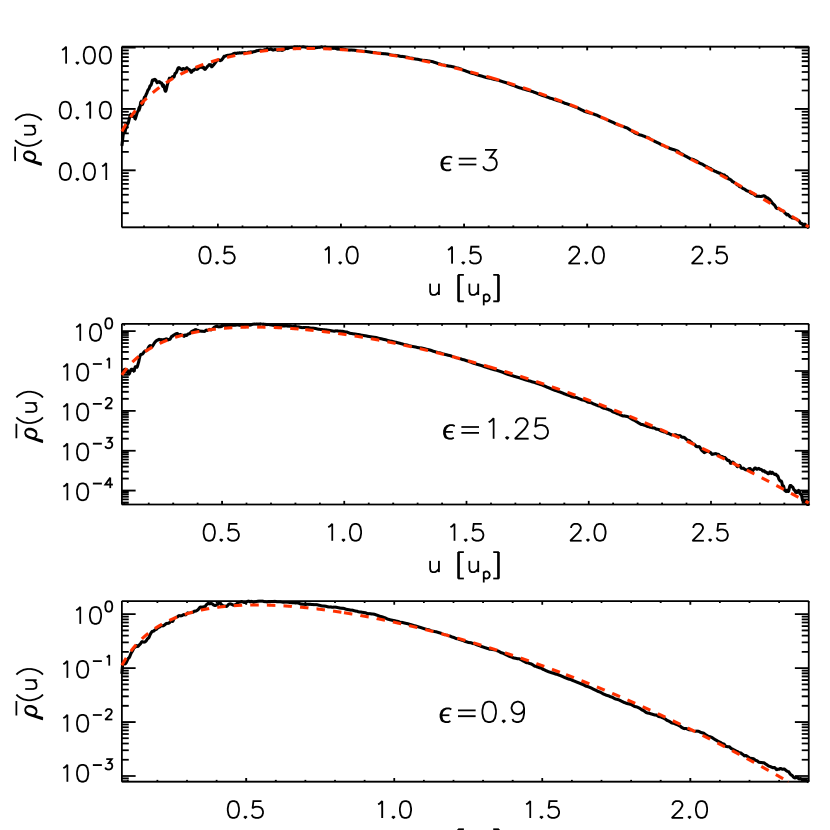
In the limit of large , the distribution of particle pairs is well fit by an equation of the form
| (8) |
as seen in Figure 6, where the fit function are the red dotted curves. However for this shape no longer fits the results, as the tail flattens, approaching a linear exponential. Equation (8) is not quite a Maxwellian probability distribution, but it is close: for we have , so the fit is nearly Maxwellian except for the high velocity tail. Note also that Equation (3) has a strict maximum which means that our tail must eventually hit zero.
4.1.3 Low , high – Exponential
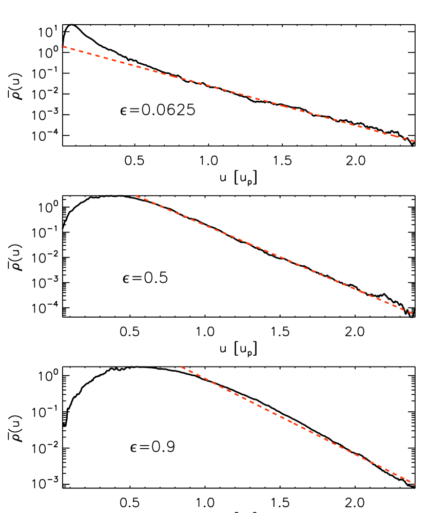
In the limit of high relative velocity , we find
| (9) |
is a good fit for low values of as shown in Figure 7, although our data range is too limited to constrain a polynomial prefactor. We show fits for ranging from to , and by the latter value the tail is clearly developing some curvature.
4.1.4 Low , low – Clustering
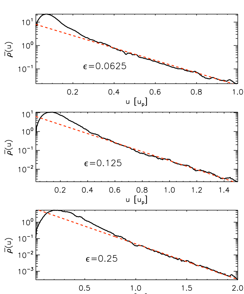
In Figure 8 we show low zooms of for our smallest runs, along with exponential fits for the higher tail. We can see that there is a distinct bump at low velocities that gets more pronounced as gets smaller. In the limit, this is the “cold” population of Paper I. Unlike that case however, for this bump in is collisional as the peak collisional velocity is located in the bump and is finite (see Figure 2, bottom panel). We attribute this enhancement to the particle pair number density at low to turbulent clustering, and therefore refer to the population as the “clustered” population.
4.2. Global fit – Form
Behavior Fitting formula quasi-Maxwellian quasi-exponential clustered
In this section we find a fit for the form of so that , that applies for all the we consider. Note that in this section, we consider only the functional form of , and allow it to depend on coefficients that are determined for each value of individually. We will fit the dependence of the coefficients on in the next section.
Combining the low results, the high results, and Figure 4, we can see that there is a qualitative change in the behavior around , which corresponds to nearly a full order of magnitude in the mass ratio of the particles. This is interesting as by that scale particle-particle collisions can no longer be considered to occur between near-equals, and the larger grain has an increased chance of surviving even fairly energetic collisions. This change in behavior can be understood through Figure 2: a particle pair with relative velocity samples a maximum separation of order . Particle pairs with see low velocity collisions that sample volumes well contained within a single eddy (or in our synthetic turbulence, a single gas velocity wavelength), while higher pairs can sample multiple eddies. This implies that analytical approaches to particle collisional velocities can only be applied to large values: if particles begin their final approach when well separated, they do not start strongly correlated and an ensemble averaging approach can be used. If their final approach begins at a small separation however, then the initial conditions are critical and contain long time correlations which cannot yet be analytically treated.
N/A N/A N/A N/A N/A N/A N/A N/A N/A N/A N/A N/A N/A N/A N/A N/A N/A N/A
Our global fit model tries to capture the quasi-Maxwellian behavior at high in a term , the quasi-exponential high- tails at low in a term and the low velocity cluster for low in a term , so our fit for is made up of
| (10) |
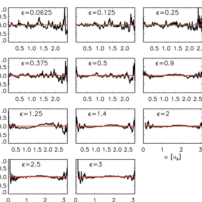
We will refer to the populations captured by the terms in order as quasi-Maxellian, quasi-exponential and clustered. The forms for and are shown in Table 2, where the parameters are amplitudes (note that the quasi-Maxwellian and quasi-exponential tail components are imperfectly normalized), the parameters are offsets and the parameters are inverse velocity scales. While the offset parameters have proven important to the fits, and both the quasi-Maxwellian and quasi-exponential behavior is seen, eight fitting parameters allow for too much freedom: fitting the parameters for Runs A-K (using starting values from Table 4), we find values tabulated in Table 3, which shows some trends, but is not generally directly useful (for example, the scatter in and is large). The fit quality is good however, as seen in Figure 9, where we plot .
4.3. Master fit
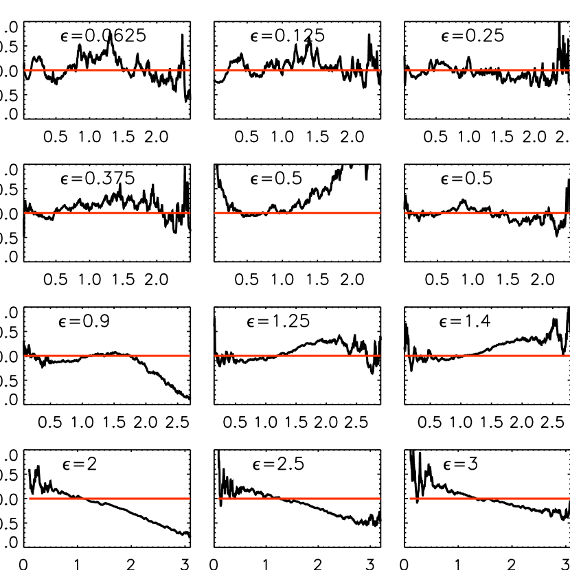
The values for the coefficients in Table 3 do not vary smoothly and monotonically with , which implies that our fit formula is not a perfect match for the data. Nonetheless, we can construct a fit for the coefficients as a function of which matches the data acceptably. Such a fit can then be adapted to generate an approximate for any , and so can be used in a particle growth model.
Requiring that for , which forces the peak of the clustered population to occur for , we can find fit formula in terms of alone, arriving at Table 4 (certainly not unique), which identifies three regimes: a large regime where the clustering term is insignificant, and two small regimes where it is important. Significantly, and do not vary for small : in this range the large tail is controlled by the exponential terms, and they have converged as a function of stopping time ratio.
We show the error of this fit in Figure 10, where we plot , which is, unsurprisingly, inferior to that in Figure 9 because the latter has full freedom for the coefficients of . While for we underestimate , it is clear that for larger our formula for does not approach the unity found in Table 3 rapidly enough. Less obviously, the formula for is imperfectly normalized. We know from Figure 3 that the integral of should be approximately in the large regime. For , we have , but for larger it rapidly approaches its asymptotic value of . Those interested in such values should consider normalizing directly.
range N/A
5. Conclusions
We have extended the work of Paper I to find turbulence induced collision rates and velocities between particles with different stopping times (i.e. of different sizes). Broadly, we find that the collisional velocity probability distribution is approximately Maxwellian for large stopping time ratios, but deviates strongly from that limit for particles with stopping time ratios less than (which corresponds to mass ratios below ). We also find, similarly to Paper I, that our collisional velocities are smaller than previously estimated (Ormel & Cuzzi, 2007) for particles with modest stopping time ratios, although the previous estimates are not bad when the particles are significantly different in size.
Further, we have managed to construct a usable estimate for the collision rates and velocities between dust grains of different sizes in turbulent flows which captures their qualitative behavior for arbitrary stopping time ratio (see Paper I for the case of monodisperse particles).
We interpret our results by noting that particle pairs with stopping time ratios close to unity (so particles of similar sizes) collide at low speeds. This means that they started their “final approach” while close together. The change in behavior between quasi-Maxwellian and non-Maxwellian collisional velocity probability distributions occurs approximately when particle pairs start their final approach one eddy size apart. This is the difference between particles whose positions and velocities have been correlated for a significant time, and particles which are nearly uncorrelated. Under that interpretation, it is hardly surprising that the collisional velocity probability distributions are different, nor that the large stopping time ratio collisions are quasi-Maxwellian.
We find a counterpart to the cold, collisionless population of Paper I (collisions between particles of identical stopping times), in our clustered population. In the case of non-unity stopping time ratios however, this population is collisional: the finite difference in stopping times forbids perfect correlation between the dust grains. We also find that while particles of similar stopping times are strongly concentrated by the turbulence, this clustering is unlikely to generate local dust grain density enhancements high enough above background to lead to streaming instabilities, although it is within the realm of the possible.
While the different collisional velocity probability distributions for different particle size ratios is not surprising, it is of particular interest for dust coagulation models. This is because the only effect that changing the velocity scale of collisions would have is to shift the final dust grain size, and shifting the final grain size enough that grains grow large enough to trigger gravitational instabilities or similar is implausible. Instead we want to enable more lucky dust grains to sneak through the fragmentation barrier by a fortuitous sequence of low velocity collisions before growing large enough to sweep up small grains in high velocity encounters.
Appendix A Measuring dust concentrations and collisions
In protoplanetary disks, dust grains that interact hydrodynamically with turbulence are far smaller than the smallest turbulent eddies, unlike the situation in many other systems including rain droplets in the Earth’s atmosphere (Shaw, 2003; Xu & Bodenschatz, 2008). This makes it impossible to simultaneously resolve individual particle-particle collisions along with the turbulence that stirs them. This complicates the interpretation of numerical simulations designed to study the rates and velocities of turbulence induced particle-particle collisions. Rather than actually tracking individual collisions, we must instead take periodic snap-shots of the entire system, identify interesting particle-particle pairs and convert their number, separation and relative velocities into global collision rates and collisional velocities. On the other hand, the same small size of the dust grains along with their high material density compared to the gas means that we can neglect the volume displaced by the grains, which is a significant simplification.
To convert snap-shots of the system to collisional diagnostics, we must make the fundamental assumption that for any relative velocity , there is a size scale , simultaneously much smaller than the smallest turbulence length and much larger than the dust grain radii , where in all spheres of radius constructed around test dust grains, the number density of dust grains with velocity with respect to the test grains is independent of . This assumption will be broken if new physics emerges when dust grains approach each other closely (such as mutual repulsion of negatively charged dust grains; Okuzumi 2009). If dust grains are large enough to induce wakes in the gas that affect particle-particle collisions, our assumption will also break down.
A.1. Parameters and considerations
The particles (moving with velocity ) and the gas (with velocity ) interact through the drag term
| (A1) |
where is the friction stopping time. Assume a turbulent cascade where the velocity of the turbulence at length-scale is and the turbulent correlation time (turnover time) at that scale is . While it has not yet been rigorously determined, the strong expectation is that the turbulence which is most strongly coupled to particle-particle relative motion (as opposed to bulk turbulent transport) is the turbulence at the scale where (Völk et al., 1980). In the case of pairs of particles with different stopping times it is generally believed that the largest stopping time defines the most-coupled turbulence.
A.2. Sampling method
As in Paper I and this work, take snap-shots of the particles with temporal separation , and bin particle pairs in space and relative velocity (velocity bin width ). From the binned data calculate , which is the number of particle pairs and with , , in the snap-shot taken at time t. A dropped implies summation over velocity bins while a dropped implies averaging over snap-shots.
Note that
| (A2) |
is the effective number density of particles at relative velocity in spheres of radius as seen by particles in the snapshot . The volume averaged number density of particles in a numerical simulation is however arbitrary (especially if they do not back-react on the gas), so it, along with the also arbitrary size of the velocity bin, should be scaled out:
| (A3) |
(see also Equation (5), this paper) measures the density of targets with relative velocity within distance compared to the background number density. Similarly to , for a dropped implies integration over velocity (giving the ratio of perceived number density to background) while a dropped implies a time average over snapshots. A dropped will be discussed in further detail below, but implies a limit .
A.3. Sampling rate
If the relative velocity of a particle pair is and , then that pair can appear in multiple consecutive snap-shots. This can result in over/undersampling particles in regions of particle over/underdensities. If we have a large number of snap-shots taken over a total time interval , our fundamental assumption implies that the oversampling of regions of over/underdensities will cancel. Nonetheless, it is safer to choose a sampling rate with where is the largest particle-particle separation we consider, and is the smallest relative velocity we consider.
More importantly, turbulence generates significant structure in the particle distribution, which can take multiple particle stopping times or turbulent turn-overs to saturate, and leads to large swings in , as seen in Paper I. As such, it is crucial to sample across multiple particle stopping times and multiple turbulent turnovers of the largest eddies which significantly interact with the dust grains.
A.4. Sampling radii
If , then the drag force will significantly affect the relative motion of particle pairs with a separation before they could collide. This implies that for any collisional sphere radius considered, there is a minimum velocity for which one can extract collisional information. Given that particle relative velocities are expected to couple most strongly to turbulence with turnover time , this immediately implies that a collisional sphere of the same size scale of that turbulence, , will not be able to resolve collisional velocities of or less. This is a strong constraint: to calculate collision rates and collision velocities (especially modest velocities) for dust grains, we need to resolve particle separations much smaller than the length scale associated with the turbulence expected to maximally couple to the particle-particle relative motions. See the discussion of the “cold” population in Paper I for a particularly interesting consequence for particles with equal stopping times.
Appendix B Method
Taking the above considerations into account, one arrives at the procedure for extracting collisional diagnostics from the snap-shots.
-
•
Examine the time series of to verify that one is sampling a particle population whose collisional parameters have achieved a steady state, and that the sampling window is long enough to average over long-time fluctuations.
-
•
Take the limit for all values of where this is possible, taking into account the requirement that . Where this is possible, the assumption is that one has achieved . Where it is not possible, either one has or the length scale does not exist. In the latter case, it is not clear how collisional diagnostics could be designed without resolving individual particle-particle collisions.
B.1. Concentrations and rates
-
•
is the number density of particles within spheres of radius seen by test particles. If particles are clustered, while if they are segregated at a lengthscale .
-
•
is the effective number density of particles with relative velocity that interact with test grains. Note both that it has units of density times inverse velocity and that it is not the term to use for collision rates!
-
•
is the contribution of the collisional velocity to the collision rate for a single particle, where is the particle-particle collisional cross-section. Note the factor of , which accounts for the fact that particles moving slowly with respect to one another will collide only on long time scales.
-
•
is the total collision rate for a single particle
-
•
is the root-mean-squared particle-particle collisional velocity.
References
- Barge & Sommeria (1995) Barge, P., & Sommeria, J. 1995, A&A, 295, L1
- Bec et al. (2010) Bec, J., Biferale, L., Cencini, M., Lanotte, A. S., & Toschi, F. 2010, Journal of Fluid Mechanics, 646, 527
- Blum & Wurm (2008) Blum, J., & Wurm, G. 2008, ARA&A, 46, 21
- Carballido et al. (2008) Carballido, A., Stone, J. M., & Turner, N. J. 2008, MNRAS, 386, 145
- Cuzzi et al. (2001) Cuzzi, J. N., Hogan, R. C., Paque, J. M., & Dobrovolskis, A. R. 2001, ApJ, 546, 496
- Cuzzi & Hogan (2003) Cuzzi, J. N., & Hogan, R. C. 2003, Icarus, 164, 127
- Dullemond & Dominik (2005) Dullemond, C. P., & Dominik, C. 2005, A&A, 434, 971
- Fessler et al. (1994) Fessler, J. R., Kulick, J. D., & Eaton, J. K. 1994, Physics of Fluids, 6, 3742
- Garaud et al. (2012) Garaud, P., Meru, F., Galvagni, M., & Olczak, C. 2012, arXiv:1209.0013
- Goldreich & Ward (1973) Goldreich, P., & Ward, W. R. 1973, ApJ, 183, 1051
- Güttler et al. (2010) Güttler, C., Blum, J., Zsom, A., Ormel, C. W., & Dullemond, C. P. 2010, A&A, 513, A56
- Hubbard (2012) Hubbard, A. 2012, MNRAS, 426, 784
- Johansen et al. (2004) Johansen, A., Andersen, A. C., & Brandenburg, A. 2004, A&A, 417, 361
- Johansen et al. (2006) Johansen, A., Klahr, H., & Henning, T. 2006, ApJ, 636, 1121
- Johansen et al. (2007) Johansen, A., Oishi, J. S., Mac Low, M.-M., Klahr, H., Henning, T., & Youdin, A. 2007, Nature, 448, 1022
- Johansen et al. (2009) Johansen, A., Youdin, A., & Mac Low, M.-M. 2009, ApJ, 704, L75
- Kolmogorov (1941) Kolmogorov, A. 1941, Akademiia Nauk SSSR Doklady, 30, 301
- Markiewicz et al. (1991) Markiewicz, W. J., Mizuno, H., & Völk, H. J. 1991, A&A, 242, 286
- Maxey (1987) Maxey, M. R. 1987, Journal of Fluid Mechanics, 174, 441
- Okuzumi (2009) Okuzumi, S. 2009, ApJ, 698, 1122
- Okuzumi et al. (2011) Okuzumi, S., Tanaka, H., Takeuchi, T., & Sakagami, M.-a. 2011, ApJ, 731, 95
- Ormel & Cuzzi (2007) Ormel, C. W., & Cuzzi, J. N. 2007, A&A, 466, 413
- Pan et al. (2011) Pan, L., Padoan, P., Scalo, J., Kritsuk, A. G., & Norman, M. L. 2011, arXiv:1106.3695
- Russell et al. (2006) Russell, S. S., Hartmann, L., Cuzzi, J., Krot, A. N., Gounelle, M., & Weidenschilling, S. 2006, Meteorites and the Early Solar System II, 233
- Shakura & Sunyaev (1973) Shakura, N. I., & Sunyaev, R. A. 1973, A&A, 24, 337
- Shaw (2003) Shaw, R. A. 2003, Annual Review of Fluid Mechanics, 35, 183
- Shi & Chiang (2013) Shi, J.-M., & Chiang, E. 2013, ApJ, 764, 20
- Toschi & Bodenschatz (2009) Toschi, F., & Bodenschatz, E. 2009, Annual Review of Fluid Mechanics, 41, 375
- Völk et al. (1980) Völk, H. J., Jones, F. C., Morfill, G. E., & Roeser, S. 1980, A&A, 85, 316
- Windmark et al. (2012) Windmark, F., Birnstiel, T., Ormel, C. W., & Dullemond, C. P. 2012, A&A, 544, L16
- Xu & Bodenschatz (2008) Xu, H., & Bodenschatz, E. 2008, Physica D Nonlinear Phenomena, 237, 2095
- Youdin & Goodman (2005) Youdin, A. N., & Goodman, J. 2005, ApJ, 620, 459
- Zsom et al. (2010) Zsom, A., Ormel, C. W., Güttler, C., Blum, J., & Dullemond, C. P. 2010, A&A, 513, A57