Planck 2013 results. XX. Cosmology from Sunyaev–Zeldovich cluster counts

We present constraints on cosmological parameters using number counts as a function of redshift for a sub-sample of 189 galaxy clusters from the Planck SZ (PSZ) catalogue. The PSZ is selected through the signature of the Sunyaev–Zeldovich (SZ) effect, and the sub-sample used here has a signal-to-noise threshold of seven, with each object confirmed as a cluster and all but one with a redshift estimate. We discuss the completeness of the sample and our construction of a likelihood analysis. Using a relation between mass $M$ and SZ signal $Y$ calibrated to X-ray measurements, we derive constraints on the power spectrum amplitude $\sigma_{8}$ and matter density parameter $\Omega_{\mathrm{m}}$ in a flat $\Lambda$CDM model. We test the robustness of our estimates and find that possible biases in the $Y$–$M$ relation and the halo mass function are larger than the statistical uncertainties from the cluster sample. Assuming the X-ray determined mass to be biased low relative to the true mass by between zero and 30%, motivated by comparison of the observed mass scaling relations to those from a set of numerical simulations, we find that $\sigma_{8}=0.75\pm 0.03$, $\Omega_{\mathrm{m}}=0.29\pm 0.02$, and $\sigma_{8}(\Omega_{\mathrm{m}}/0.27)^{0.3}=0.764\pm 0.025$. The value of $\sigma_{8}$ is degenerate with the mass bias; if the latter is fixed to a value of 20% (the central value from numerical simulations) we find $\sigma_{8}(\Omega_{\mathrm{m}}/0.27)^{0.3}=0.78\pm 0.01$ and a tighter one-dimensional range $\sigma_{8}=0.77\pm 0.02$. We find that the larger values of $\sigma_{8}$ and $\Omega_{\mathrm{m}}$ preferred by Planck’s measurements of the primary CMB anisotropies can be accommodated by a mass bias of about $40\%$. Alternatively, consistency with the primary CMB constraints can be achieved by inclusion of processes that suppress power on small scales relative to the $\Lambda$CDM model, such as a component of massive neutrinos. We place our results in the context of other determinations of cosmological parameters, and discuss issues that need to be resolved in order to make further progress in this field.

Figure 1: Distribution on the sky of the Planck SZ cluster sub-sample used in this paper, with the 35% mask overlaid.

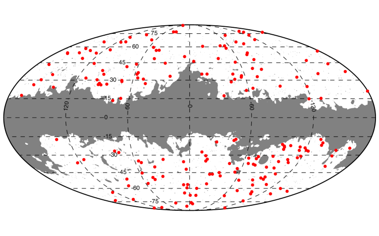
1 Introduction

This paper, one of a set associated with the 2013 release of data from the Planck mission (Planck Collaboration I, 2014), describes the constraints on cosmological parameters using number counts as a function of redshift for a sample of 189 galaxy clusters.

Within the standard picture of structure formation, galaxies aggregate into clusters of galaxies at late times, forming bound structures at locations where the initial fluctuations create the deepest potential wells. The study of these galaxy clusters has played a significant role in the development of cosmology over many years (see, for example, Perrenod 1980, Oukbir & Blanchard 1992, White et al. 1993, Carlberg et al. 1996, Voit 2005, Henry et al. 2009, Vikhlinin et al. 2009b and Allen et al. 2011). More recently, as samples of clusters have increased in size and variety, number counts inferred from tightly-selected surveys have been used to obtain detailed constraints on the cosmological parameters.

The early galaxy cluster catalogues were constructed by eye from photographic plates with a ‘richness’ (or number of galaxies) attributed to each cluster (Abell, 1958; Abell et al., 1989). As time has passed, new approaches for selecting clusters have been developed, most notably using X-ray emission due to thermal Bremsstrahlung radiation from the hot gas that makes up most of the baryonic matter in the cluster. X-ray cluster surveys include both the NORAS (Böhringer et al., 2000) and REFLEX (Böhringer et al., 2004) surveys, based on ROSAT satellite observations, which have been used as source catalogues for higher-precision observations by the Chandra and XMM-Newton satellites, as well as surveys with XMM-Newton, including the XMM Cluster Survey (XCS, Mehrtens et al. 2012) and the XMM Large Scale Structure survey (XMM-LSS, Willis et al. 2013).

To exploit clusters for cosmology, a key issue is how the properties used to select and characterize the cluster are related to the total mass of the cluster, since this is the quantity most readily predicted using theoretical models. Galaxies account for a small fraction of the cluster mass, and the scatter between richness and mass appears to be large. However, there are a number of other possibilities. In particular, there are strong correlations between the total mass and both the integrated X-ray surface brightness and X-ray temperature, making them excellent mass proxies.

The Sunyaev–Zeldovich (SZ) effect (Sunyaev & Zeldovich, 1970; Zeldovich & Sunyaev, 1969) is the inverse Compton scattering of cosmic microwave background (CMB) photons by the hot gas along the line of sight, and this is most significant when the line of sight passes through a galaxy cluster. It leads to a decrease in the overall brightness temperature in the Rayleigh–Jeans portion of the spectrum and an increase in the Wien tail, with a null around $217\thinspace{\mathrm{GHz}}$ (see Birkinshaw 1999 for a review). The amplitude of the SZ effect is given by the integrated pressure of the gas within the cluster along the line of sight. Evidence both from observation (Marrone et al., 2012; Planck Collaboration Int. III, 2013) and from numerical simulations (Springel et al., 2001; da Silva et al., 2004; Motl et al., 2005; Nagai, 2006; Kay et al., 2012) suggests that the SZ effect is an excellent mass proxy. A number of articles have discussed the possibility of using SZ-selected cluster samples to constrain cosmological parameters (Barbosa et al., 1996; Aghanim et al., 1997; Haiman et al., 2001; Holder et al., 2001; Weller et al., 2002; Diego et al., 2002; Battye & Weller, 2003).

This paper describes the constraints on cosmological parameters imposed by a high signal-to-noise (S/N) sub-sample of the Planck SZ Catalogue (PSZ, see Planck Collaboration XXIX 2014, henceforth Paper 1, for details of the entire catalogue) containing nearly 200 clusters (shown in Fig. 1). This sub-sample has been selected to be pure, in the sense that all the objects within it have been confirmed as clusters via additional observations, either from the literature or undertaken by the Planck collaboration. In addition all objects but one have a measured redshift, either photometric or spectroscopic. This is the largest SZ-selected sample of clusters used to date for this purpose. We will show that it is the systematic uncertainties from our imperfect knowledge of cluster properties that dominate the overall uncertainty on cosmological constraints.

The Planck cluster sample is complementary to those from observations using the South Pole Telescope (SPT, Carlstrom et al. 2011) and the Atacama Cosmology Telescope (ACT, Swetz et al. 2011), whose teams recently published the first large samples of SZ-selected clusters (Reichardt et al., 2013; Hasselfield et al., 2013). The resolution of Planck at the relevant frequencies is between 5 and 10 arcmin, whereas that for ACT and SPT is about $1\thinspace{\mathrm{arcmin}}$, but the Planck sky coverage is much greater. This means that Planck typically finds larger, more massive, and lower-redshift clusters than those found by SPT and ACT.

Our strategy is to focus on number counts of clusters, as a function of redshift, above a high S/N threshold of seven and to explore the robustness of the results. We do not use the observed SZ brightness of the clusters, due to the significant uncertainty caused by the size–flux degeneracy as discussed in Paper 1. Accordingly, our theoretical modelling of the cluster population is directed only at determining the expected number of clusters in each redshift bin exceeding the S/N threshold. The predicted and observed numbers of clusters are then compared in order to obtain the likelihood. In the future, we will make use of the SZ-estimated mass and a larger cluster sample to extend the analysis to broader cosmological scenarios.

This paper is laid out as follows. We describe the theoretical modelling of the redshift number counts in Sect. 2, while Sect. 3 presents the PSZ cosmological sample and selection function used in this work. The likelihood we adopt for putting constraints on cosmological parameters is given in Sect. 4. Section 5 presents our results on cosmological parameter estimation and assesses their robustness. We discuss how they fit in with other cluster and cosmological constraints in Sect. 6, before providing a final summary. A detailed discussion of our calibration of the SZ flux versus mass relation and its uncertainties is given in Appendix A.

2 Modelling cluster number counts

2.1 Model definitions

We parameterize the standard cosmological model as follows. The densities of various components are specified relative to the present-day critical density, with $\Omega_{\mathrm{X}}=\rho_{\mathrm{X}}/\rho_{\mathrm{crit}}$ denoting that for component X. These components always include matter, $\Omega_{\mathrm{m}}$, and a cosmological constant $\Omega_{\Lambda}$. For this work we assume that the Universe is flat, that is, $\Omega_{\mathrm{m}}+\Omega_{\Lambda}=1$, and the optical depth to reionization is fixed at $\tau=0.085$ except in the CMB+SZ analyses. The present-day expansion rate of the Universe is quantified by the Hubble constant $H_{0}=100\thinspace h\thinspace{\mathrm{km}}\thinspace{\mathrm{s}}^{-1}\thinspace{\mathrm{Mpc}}^{-1}$.

The cluster number counts are very sensitive to the amplitude of the matter power spectrum. When studying cluster counts it is usual to parametrize this in terms of the density variance in spheres of radius $8h^{-1}\thinspace\mathrm{Mpc}$, denoted $\sigma_{8}$, rather than overall power spectrum amplitude, $A_{\mathrm{s}}$. In cases where we include primary CMB data we use $A_{\mathrm{s}}$ and compute $\sigma_{8}$ as a derived parameter. In addition to the parameters above, we allow the other standard cosmological parameters to vary: $n_{\mathrm{s}}$ representing the spectral index of density fluctuations; and $\Omega_{\mathrm{b}}h^{2}$ quantifying the baryon density.

The number of clusters predicted to be observed by a survey in a given redshift interval $[z_{i},z_{i+1}]$ can be written

$$n_{i}=\int_{z_{i}}^{z_{i+1}}dz{dN\over dz},$$ (1)

with

$${dN\over dz}=\int d\Omega\int dM_{500}\thinspace\hat{\chi}(z,M_{500},l,b)\thinspace{dN\over dz\thinspace dM_{500}\thinspace d\Omega}\thinspace,$$ (2)

where $d\Omega$ is the solid angle element and $M_{500}$ is the mass within the radius where the mean enclosed density is 500 times the critical density. The quantity $\hat{\chi}(z,M_{500},l,b)$ is the survey completeness at a given location $(l,b)$ on the sky, given by

$$\hat{\chi}=\int dY_{500}\int d\theta_{500}P(z,M_{500}|Y_{500},\theta_{500})\thinspace\chi(Y_{500},\theta_{500},l,b)\thinspace.$$ (3)

Here $P(z,M_{500}|Y_{500},\theta_{500})$ is the distribution of $(z,M_{500})$ for a given $(Y_{500},\theta_{500})$, where $Y_{500}$ and $\theta_{500}$ are the SZ flux and size of a cluster of redshift and mass $(z,M_{500})$.

This distribution is obtained from the scaling relations between $Y_{500}$, $\theta_{500}$, and $M_{500}$, discussed later in this section. Note that $\hat{\chi}(z,M_{500},l,b)$ depends on cosmological parameters through $P(z,M_{500}|Y_{500},\theta_{500})$, while the completeness in terms of the observables, $\chi(Y_{500},\theta_{500},l,b)$, does not depend on the cosmology as it refers directly to the observed quantities.

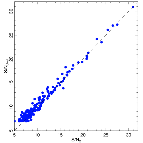
For the present work, we restrict our analysis to the quantity $dN/dz$ that measures the total counts in redshift bins. In particular, we do not use the blind SZ flux estimated by the cluster candidate extraction methods that, as detailed in Planck Collaboration VIII (2011), is found to be significantly higher than the flux predicted from X-ray measurements. In contrast to the blind SZ flux, the blind S/N is in good agreement with the S/N measured using X-ray priors. Figure 2 shows the blind S/N (S/N_blind) versus the S/N re-extracted at the X-ray position and using the X-ray size (S/N_X). The clusters follow the equality line. In Sect. 3, we use the (S/N_blind) values to define our cosmological sample, while for the predicted counts (defined in Sect. 2) we use the completeness based on S/N_X. Our analysis relies on the good match between these two quantities.

Figure 2: Blind S/N versus S/N re-extracted at the X-ray position using the X-ray size, for the MMF3 detections of Planck clusters that are associated with known X-ray clusters in the reference cosmological sample. In contrast to the blind SZ flux, the blind S/N is in good agreement with S/N measured using X-ray priors.

To carry out a prediction of the counts expected in a survey, given cosmological assumptions, we therefore need the following inputs:

• a mass function that tells us the number distribution of clusters with mass and redshift;

• scaling relations that can predict observable quantities from the mass and redshift;

• the completeness of the survey in terms of those observables, which tells us the probability that a model cluster would make it into the survey catalogue.

These are described in the remainder of this section and in the next.

2.2 Mass function

Our main results use the mass function from Tinker et al. (2008), giving the number of haloes per unit volume:

$${dN\over dM_{500}}(M_{500},z)=f(\sigma)\thinspace{\rho_{\mathrm{m}}(z=0)\over M_{500}}\thinspace{d\ln\sigma^{-1}\ \over dM_{500}}\thinspace,$$ (4)

where

$$f(\sigma)=A\left[1+\left({\sigma\over b}\right)^{-a}\right]\exp\left(-{c\over\sigma^{2}}\right)\thinspace,$$ (5)

and ${\rho}_{\mathrm{m}}(z=0)$ is the mean matter density at $z=0$. The coefficients $A$, $a$, $b$ and $c$ are tabulated in Tinker et al. (2008) for different overdensities, $\Delta_{\mathrm{mean}}$, with respect to the mean cosmic density, and depend on $z$. Here we use $\Delta_{\mathrm{critical}}=500$ relative to the critical density, so we compute the relevant mass function coefficients by interpolating the Tinker et al. (2008) tables for haloes with $\Delta_{\mathrm{mean}}\equiv\Delta_{\mathrm{critical}}/\Omega_{\mathrm{m}}(z)=500/\Omega_{\mathrm{m}}(z)$, where $\Omega_{\mathrm{m}}(z)$ is the matter density parameter at redshift $z$.

The quantity $\sigma$ is the standard deviation, computed in linear perturbation theory, of the density perturbations in a sphere of radius $R$, which is related to the mass by $M=4\pi\rho_{\mathrm{m}}(z=0)R^{3}/3$. It is given by

$$\sigma^{2}=\frac{1}{2\pi^{2}}\int dk\thinspace k^{2}P(k,z)|W(kR)|^{2}\thinspace,$$ (6)

where $P(k,z)$ is the matter power spectrum at redshift $z$, which we compute for any given set of cosmological parameters using CAMB (Lewis et al., 2000), and $W(x)=3(\sin x-x\cos x)/x^{3}$ is the filter function of a spherical top hat of radius $R$.

The quantity $dN/(dz\thinspace dM_{500}\thinspace d\Omega)$ in Eq. 2 is computed by multiplying the mass function $dN(M_{500},z)/dM_{500}$ by the volume element $dV/(dz\thinspace d\Omega)$.

As a baseline we use, except where stated otherwise, the Tinker et al. (2008) mass function, but we consider an alternative mass function as a cross-check. In a recent publication by Watson et al. (2013), a new mass function is extracted from the combination of large cosmological simulations (typical particle numbers of $3000^{3}$ to $6000^{3}$) with a very large dynamic range (size from $11\thinspace h^{-1}$ to $6000\thinspace h^{-1}$Mpc), which extends the maximum volume probed by Tinker et al. by two orders of magnitude. The two mass functions agree fairly well, except in the case of the most massive objects, where Tinker et al.’s mass function predicts more clusters than Watson et al.’s. The Tinker et al. mass function might be derived from volumes that are not large enough to properly sample the rarer clusters. These rare clusters are more relevant for Planck than for ground-based SZ experiments, which probe smaller areas of the sky. The Watson et al. mass function is used only in Sect. 5.3, which deals with mass function uncertainties.

2.3 Scaling relations

A key issue is to relate the observed SZ flux, $Y_{500}$, to the mass $M_{500}$ of the cluster. As we show in Sect. 5, cosmological constraints are sensitive to the normalization, slope and scatter of the assumed $Y_{500}$–$M_{500}$ relation. We thus paid considerable attention to deriving the most accurate scaling relations possible, with careful handling of statistical and systematic uncertainties, and to testing their impact on the derived cosmological parameters.

The baseline relation is obtained from an observational calibration of the $Y_{500}$–$M_{500}$ relation on one-third of the cosmological sample. The calibration uses $M_{500}^{Y_{\mathrm{X}}}$, the mass derived from the X-ray $Y_{\mathrm{X}}$–$M_{500}$ relation, as a mass proxy. Here $Y_{\mathrm{X}}$ is the X-ray analogue of the SZ signal introduced by Kravtsov et al. (2006), as defined in Appendix A. $Y_{500}$ is then measured interior to $R_{500}^{Y_{\mathrm{X}}}$, the radius corresponding to $M_{500}^{Y_{\mathrm{X}}}$. The mean bias between $M_{500}^{Y_{\mathrm{X}}}$ and the true mass, $(1-b)$, is assumed to account for all possible observational biases (departure from hydrostatic equilibrium (HE), absolute instrument calibration, temperature inhomogeneities, residual selection bias, etc) as discussed in full in Appendix A. In practice, the plausible range for this mean bias $(1-b)$ was estimated by comparing the observed relation with predictions from several sets of numerical simulations, as detailed in Appendix A.

The large uncertainties on $(1-b)$ are due to the dispersion in predictions from the various simulation sets. This is a major factor limiting the accuracy of our analysis. A value $(1-b)=0.8$ could be considered as a best guess given available simulations, with no clear dependence on mass or redshift. From one cluster to the next the ratio of $M^{Y_{X}}_{500}$ to the true mass is expected to be stochastic, contributing to the scatter in the $Y_{500}$–$M_{500}$ relation given below. A conspiracy of all possible sources of bias (departure from HE, absolute instrument calibration, temperature inhomogeneities, residual selection bias) would seem necessary to lead to a significantly lower value of $(1-b)$. This apparently implausible possibility needs to be excluded through tests using other probes such as baryon and gas fractions, gas pressure, etc. As a baseline we take $(1-b)$ to vary within the range $[0.7,1.0]$ with a flat prior. We also consider, when analysing systematic uncertainties on the derived cosmological parameters, a case where the bias is fixed to the value $(1-b)=0.8$.

As detailed in Appendix A, we derive a baseline relation for the mean SZ signal $\bar{Y}_{500}$ from a cluster of given mass and redshift in the form

$$E^{-\beta}(z)\left[\frac{D_{\mathrm{A}}^{2}(z)\thinspace{\bar{Y}}_{500}}{\mathrm{10^{-4}\thinspace Mpc^{2}}}\right]=Y_{\ast}\left[{h\over 0.7}\right]^{-2+\alpha}\left[\frac{(1-b)\thinspace M_{\mathrm{500}}}{6\times 10^{14}\thinspace\mathrm{M}_{\odot}}\right]^{\alpha}\thinspace,$$ (7)

where $D_{\mathrm{A}}(z)$ is the angular-diameter distance to redshift $z$ and $E^{2}(z)=\Omega_{\mathrm{m}}(1+z)^{3}+\Omega_{\Lambda}$. The coefficients $Y_{\ast}$, $\alpha$, and $\beta$ are given in Table 1.

Table 1: Summary of scaling-law parameters and error budget.

Parameter      Value

$$\log Y_{\ast}$$      

     

     

     

Equation 7 has an estimated intrinsic scatter $\sigma_{\log Y}=0.075$, which we take to be independent of redshift (see Appendix A). This is incorporated by drawing the cluster’s $Y_{500}$ from a log-normal distribution

$${\mathcal{P}}(\log Y_{500})={1\over\sqrt{2\pi\sigma_{\log Y}^{2}}}\exp\left[{-\frac{\log^{2}(Y_{500}/{\bar{Y}}_{500})}{2\sigma_{\log Y}^{2}}}\right]\thinspace,$$ (8)

where ${\bar{Y}}_{500}$ is given by Eq. 7. Inclusion of this scatter increases the number of clusters expected at a given S/N; since the cluster counts are a steep function of $M_{500}$ in the range of mass in question, there are more clusters that scatter upwards from below the limit given by the zero-scatter scaling relation than those that scatter downwards.

In addition to Eq. 7 we need a relation between $\theta_{500}$ (in fact $\theta_{500}^{Y_{\mathrm{X}}}$, the angular size corresponding to the physical size $R_{500}^{Y_{\mathrm{X}}}$), the aperture used to extract $Y_{500}$, and $M_{500}$. Since $M_{500}=500\times 4\pi\rho_{\mathrm{crit}}R_{500}^{3}/3$ and $\theta_{500}=R_{500}/D_{\mathrm{A}}$, this can be expressed as

$${\bar{\theta}_{500}}=\theta_{\ast}\left[\frac{h}{0.7}\right]^{-2/3}\left[{(1-b)\thinspace M_{500}\over 3\times 10^{14}\mathrm{M}_{\odot}}\right]^{1/3}\thinspace E^{-2/3}(z)\thinspace\left[{D_{\mathrm{A}}(z)\over 500\thinspace{\mathrm{Mpc}}}\right]^{-1}\!\!,$$ (9)

where $\theta_{\ast}=6.997\thinspace\mathrm{arcmin}$.

2.4 Limiting mass

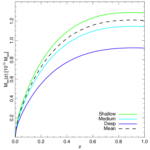
One can use Eqs. 7 and 9 to compute the limiting mass at a point on the sky where the noise level, $\sigma_{Y}$, has been computed as described in Sect. 3. As the latter is not homogeneous on the sky, we show in Fig. 3 the limiting mass, defined at 50% completeness, as a function of redshift for three different zones, deep, medium, and shallow, covering respectively, 3.5%, 47.8%, and 48.7% of the unmasked sky. For each line a S/N cut of 7 has been adopted.

Figure 3: Limiting mass as a function of $z$ for the selection function and noise level computed for three zones (deep, blue; medium, cyan; shallow, green), and on average for the unmasked sky (dashed black).

2.5 Implementation

We have implemented three independent versions of the computation of counts and constraints. The differences in predicted counts are of the order of a few percent, which translates to less than a tenth of $1\thinspace\sigma$ on the cosmological parameters of interest.

3 The Planck cosmological samples

3.1 Sample definition

The reference cosmological sample is constructed from the PSZ Catalogue published in Planck Collaboration XXIX (2014) and made public with the first release of Planck cosmological products. It is based on the SZ detections performed with the matched multi-filter (MMF) method MMF3 (Melin et al., 2006), which relies on the use of a filter of adjustable width $\theta_{500}$ chosen to maximize the S/N of the detection. In order to ensure a high purity and to maximize the number of redshifts, the cosmological sample was constructed by selecting the SZ detections above a S/N threshold of 7 outside Galactic and point source masks covering 35% of the sky, as discussed in Paper 1. From the original PSZ, only the information on S/N (for the selection) and redshift are used.

This sample contains 189 candidates. All but one are confirmed bona fide clusters with measured redshifts, including 184 spectroscopic redshifts. Among these confirmed clusters 12 were confirmed with follow-up programmes conducted by the Planck collaboration (see Paper 1 for details). The remaining non-confirmed cluster candidate is a high-reliability class1 candidate, meaning that its characterization as a cluster is supported by data in other wavebands (see Paper 1 for details). It is thus considered as a bona fide cluster. The distribution on the sky of this baseline cosmological sample is shown in Fig. 1.

In addition to our reference sample, we consider two other samples drawn from the PSZ for consistency checks. One is based on the detections from the second implementation of the MMF algorithm, MMF1, described in Paper 1. It contains 188 clusters with S/N $>7$ and no missing redshifts, with almost complete overlap with the baseline sample (187 clusters in common). The third sample considered in the present study is also based on MMF3 detections but with a higher S/N cut of S/N $>8$. It allows us to test selection effects and to probe the consistency of the results as a function of the S/N cut. It contains 136 clusters, all with measured redshifts.

The selection function for each of these samples is constructed as described in the next section.

3.2 Completeness

The completeness of the reference cosmological sample is computed with two distinct and complementary approaches: a semi-analytic approach based on the assumption of Gaussian uncertainties, and a computational approach based on Monte Carlo cluster injection into real sky maps.

The completeness $\chi$ can be evaluated analytically by setting the probability of the measured SZ flux, $Y_{500}$, to be Gaussian distributed with a standard deviation equal to the noise, $\sigma_{Y_{500}}(\theta_{500},l,b)$, computed for each size $\theta_{500}$ of the MMF filter and at each position $(l,b)$ on the sky:

$$\chi_{\mathrm{erf}}(Y_{500},\theta_{500},l,b)=\frac{1}{2}\left[{1+{\mathrm{erf}}\left({{Y_{500}-X\thinspace\sigma_{Y_{500}}(\theta_{500},l,b)}\over{{\sqrt{2}}\thinspace\sigma_{Y_{500}}(\theta_{500},l,b)}}\right)}\right]\thinspace,$$ (10)

where $X=7$ is the S/N threshold and the error function is defined as usual by

$${\mathrm{erf}}(u)={2\over\sqrt{\pi}}\int_{0}^{u}\exp\left(-t^{2}\right)dt\thinspace.$$ (11)

$\chi_{\mathrm{erf}}(Y_{500},\theta_{500},l,b)$ thus lies in the range $[0,1]$ and gives the probability for a cluster of flux $Y_{500}$ and size $\theta_{500}$ at position $(l,b)$ to be detected at S/N $\geq X$.

Figure 4: Noise map $\sigma_{Y_{500}}(\theta_{500})$ for $\theta_{500}=6\;\mathrm{arcmin}$. The PSZ is limited by instrumental noise at high ($|b|>20^{\circ}$) Galactic latitude (deeper at ecliptic poles) and foreground noise at low Galactic latitude. The scale of the map ranges from 0.5 to 2 times the mean noise of the map, which is $\langle\sigma_{Y_{500}}(6\;\mathrm{arcmin})\rangle=2.2\times 10^{-4}\mathrm{arcmin}^{2}$.

The noise estimate $\sigma_{Y_{500}}(\theta_{500},l,b)$ is a by-product of the detection algorithm and can be written in the form (see e.g., Melin et al. 2006)

$$\sigma_{Y_{500}}(\theta_{500},l,b)=\left[\int d^{2}k\;\@vec{F}_{\theta_{500}}^{t}(\@vec{k})\cdot\@vec{P}^{-1}(\@vec{k},l,b)\cdot\@vec{F}_{\theta_{500}}(\@vec{k})\right]^{-1/2}\thinspace,$$ (12)

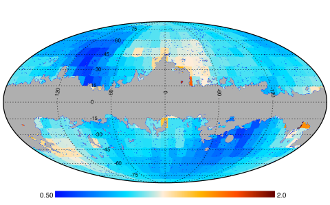
with $\@vec{F}_{\theta_{500}}(\@vec{k})$ being a vector of dimension $N_{\mathrm{freq}}$ (the six highest Planck frequencies here) containing the beam-convolved cluster template scaled to the known SZ frequency dependence. The cluster template assumed is the non-standard universal pressure profile from Arnaud et al. (2010). $\@vec{P}(\@vec{k},l,b)$ is the noise power spectrum (dimension $N_{\mathrm{freq}}\times N_{\mathrm{freq}}$) directly estimated from the data at position $(l,b)$. Figure 4 shows $\sigma_{Y_{500}}(\theta_{500},l,b)$ for $\theta_{500}=6\thinspace{\mathrm{arcmin}}$ in a Mollweide projection with the Galactic mask used in the analysis applied. As expected, the noise at high Galactic latitude is lower than in the areas contaminated by diffuse Galactic emission. The ecliptic pole regions have the lowest noise level, reflecting the longer Planck integration time in these high-redundancy areas.

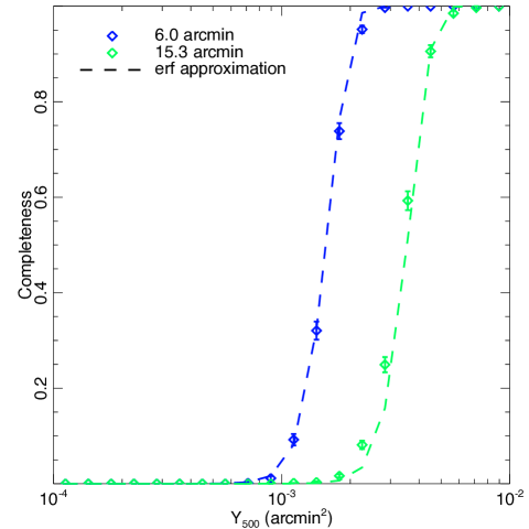
The Monte Carlo (MC) completeness is calculated by injecting simulated clusters into real sky maps following the method presented in Paper 1, with the modifications that the 65% Galactic dust mask and a S/N $>7$ threshold are applied to match the cosmological sample definition. The Monte Carlo completeness encodes effects not probed by the erf approximation, including the variation of cluster pressure profiles around the fiducial pressure profile used in the MMF, spatially-varying and asymmetric effective beams, and the effects of correlated non-Gaussian uncertainties in the estimation of $(Y_{500},\theta_{500})$. As shown in Fig. 5, the erf-based formula for the completeness is a good approximation to the Monte Carlo completeness. The agreement is best for the typical sizes probed by Planck (5 to 10 arcmin), though the two determinations of the completeness start to deviate for small and large sizes, due to beam and profile effects, respectively. For simplicity, we chose the erf formulation as the baseline. The effect of using the Monte Carlo completeness instead is discussed in Sect. 5.2.

Figure 5: Completeness averaged over the unmasked sky as a function of $Y_{500}$ for two different filter sizes, $\theta_{500}=6$ and $15.3$ arcmin. The dashed lines show the semi-analytic approximation of Eq. 10, while the diamonds with errors show the completeness estimated by the MC injection technique.

Table 2: Best-fit cosmological parameters for various combinations of data and analysis methods.

Data      $$\sigma_{8}(\Omega_{\mathrm{m}}/0.27)^{0.3}$$                  

Planck SZ +BAO+BBN                        [0.7,1]

Planck SZ +HST+BBN                        [0.7,1]

Planck SZ +BAO+BBN                        

MMF1 sample +BAO+BBN                        

MMF3 S/N +BAO+BBN                        

Planck SZ +BAO+BBN (MC completeness)                        

Planck SZ +BAO+BBN (Watson et al. mass function)                        

4 Likelihood and Markov chain Monte Carlo

4.1 The likelihood

We now have all the information needed to predict the counts in redshift bins for our theoretical models. To obtain cosmological constraints with the PSZ sample presented in Sect. 3, we construct a likelihood function based on Poisson statistics (Cash, 1979):

$$\ln L=\ln\mathcal{P}(N_{i}|n_{i})=\sum_{i=1}^{N_{\mathrm{b}}}[N_{i}\ln(n_{i})-n_{i}-\ln(N_{i}!)]\thinspace,$$ (13)

where $\mathcal{P}(N_{i}|n_{i})$ is the probability of finding $N_{i}$ clusters in each of $N_{\mathrm{b}}$ bins given an expected number of $n_{i}$ in each bin in redshift. The likelihood includes bins that contain no observed clusters. As a baseline, we assume bins in redshift of $\Delta z=0.1$ and we checked that our results are robust when changing the bin size between $0.05$ and $0.2$. The modelled expected number $n_{i}$ depends on the bin range in redshift and on the cosmological parameters, as described in Sect. 2. It also depends on the scaling relations and the selection function of the observed sample. The parameters of the scaling relations between flux (or size) and mass and redshift are taken to be Gaussian distributed with central values and uncertainties stated in Table 1, and with the scatter in $Y_{500}$ incorporated into the method via the log-normal distribution with width $\sigma_{\log Y}$.

Figure 6: Planck SZ constraints (+BAO+BBN) on $\Lambda$CDM cosmological parameters in red. The black lines show the constraints upon substituting HST constraints on $H_{0}$ for the BAO constrainsts. Contours are 68 and 95% confidence levels.

In the PSZ, the redshifts have been collected from different observations and from the literature. Individual uncertainties in redshift are thus spread between 0.001 and 0.1. Most of the clusters in the cosmological sample have spectroscopic redshifts (184 out of 189) and we checked that the uncertainties in redshift are not at all dominant in our error budget; they are thus neglected. The cluster without known redshift is incorporated by scaling the counts by a factor 189/188, i.e., by assuming its redshift is drawn from the distribution defined by the other 188 objects.

4.2 Markov chain Monte Carlo

In order to impose constraints on cosmological parameters from our sample(s) given our modelled expected number counts, we modified CosmoMC (Lewis & Bridle, 2002) to include the likelihood described above. We mainly study constraints on the spatially-flat $\Lambda$CDM model, varying $\Omega_{\mathrm{m}}$, $\sigma_{8}$, $\Omega_{\mathrm{b}}$, $H_{0}$, and $n_{\mathrm{s}}$, but also adding in the total neutrino mass, $\sum m_{\nu}$, in Sect. 6. In each of the runs, the nuisance parameters ($Y_{\ast}$, $\alpha$, $\sigma_{\log Y}$) follow Gaussian priors, with the characteristics detailed in Table 1, and are marginalized over. The bias $(1-b)$ follows a flat prior in the range [0.7,1]. The redshift evolution of the scaling, $\beta$, is fixed to its reference value unless stated otherwise.

4.3 External datasets

When probing the six parameters of the $\Lambda$CDM model, we combine the Planck clusters with the Big Bang nucleosynthesis (BBN) constraints from Steigman (2008), $\Omega_{\mathrm{b}}h^{2}=0.022\pm 0.002$. We also use either the $H_{0}$ determination from HST by Riess et al. (2011), $H_{0}=(73.8\pm 2.4)$ kms^-1Mpc^-1, or baryon acoustic oscillation (BAO) data. In the latter case we adopt the combined likelihood of Hinshaw et al. (2013) and Planck Collaboration XVI (2014), which uses the radial BAO scales observed by 6dFGRS (Beutler et al., 2011), SDSS-DR7-rec and SDSS-DR9-rec (Padmanabhan et al., 2012; Anderson et al., 2012), and WiggleZ (Blake et al., 2012).

5 Constraints from Planck clusters: $\Lambda$CDM

5.1 Results for $\Omega_{\mathrm{m}}$ and $\sigma_{8}$

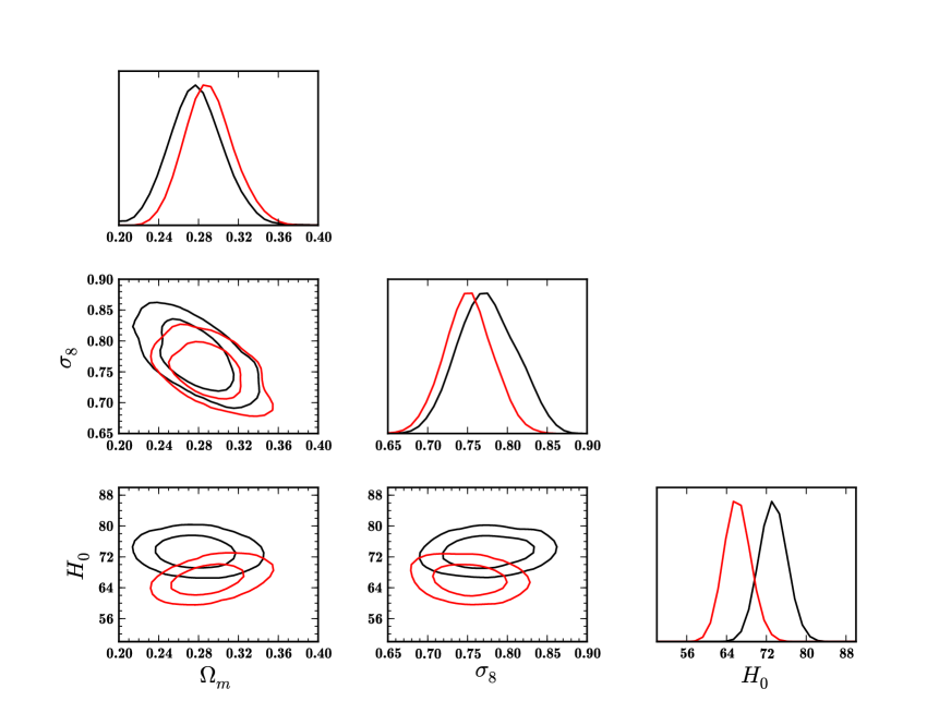
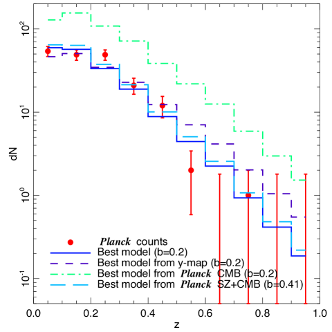
Cluster counts in redshift for our Planck cosmological sample are not sensitive to all parameters of the $\Lambda$CDM model. We focus first on ($\Omega_{\mathrm{m}},\sigma_{8}$), assuming that $n_{\mathrm{s}}$ follows a Gaussian prior centred on the best-fit Planck CMB value ($n_{\mathrm{s}}=0.9603\pm 0.0073$). We combine our SZ counts likelihood with the BAO and BBN likelihoods discussed earlier. We also incorporate the uncertainties on scaling parameters in Table 1. Allowing the bias to range uniformly over the interval $[0.7,1.0]$, we find the expected degeneracy between the two parameters, $\sigma_{8}(\Omega_{\mathrm{m}}/0.27)^{0.3}=0.764\pm 0.025$, with central values and uncertainties of $\Omega_{\mathrm{m}}=0.29\pm 0.02$ and $\sigma_{8}=0.75\pm 0.03$ (Table 2 and Fig. 6, red contours). The cluster counts as a function of redshift for the best-fit model are plotted in Fig. 7. When fixing the bias to $(1-b)=0.8$, the constraint on $\Omega_{\mathrm{m}}$ remains unchanged while the constraint on $\sigma_{8}$ becomes stronger: $\sigma_{8}(\Omega_{\mathrm{m}}/0.27)^{0.3}=0.78\pm 0.01$ and $\sigma_{8}=0.77\pm 0.02$ (Fig. 8).

Figure 7: Distribution in redshift for the Planck cosmological cluster sample. The observed number counts (red), are compared to our best-fit model prediction (blue). The dashed and dot-dashed histograms are the best-fit models from the Planck SZ power spectrum and Planck CMB power spectrum fits, respectively. The cyan long dashed histogram is the best fit CMB+SZ when the bias is free (see Section 6.3). The uncertainties on the observed counts, shown for illustration only, are the standard deviation based on the observed counts, except for empty bins where we show the inferred 84% upper limit on the predicted counts assuming a Poissonian distribution. See Sect. 6 for more discussion.

Figure 8: Comparison of the constraints using the mass functions of Watson et al. (black) and Tinker et al. (red), with $b$ fixed to 0.8. When relaxing the constraints on the evolution of the scaling law with redshift (blue), the contours move along the degeneracy line. Allowing the bias to vary uniformly in the range $[0.7,1.0]$ enlarges the constraints perpendicular to the $\sigma_{8}$–$\Omega_{\mathrm{m}}$ degeneracy line due to the degeneracy of the number of clusters with the mass bias (purple). Contours are 95% confidence levels here.

To investigate how robust our results are when changing our priors, we repeat the analysis substituting the HST constraints on $H_{0}$ for the BAO results. Figure 6 (black contours) shows that the main effect is to change the best-fit value of $H_{0}$, leaving the $(\Omega_{\mathrm{m}},\sigma_{8})$ degeneracy almost unchanged. In the following robustness tests, we assume a fixed mass bias, $(1-b)=0.8$, to better identify the effect of each of our assumptions.

5.2 Robustness to the observational sample

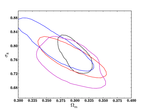
To test the robustness of our results, we performed the same analysis with different sub-samples drawn from our cosmological sample or from the PSZ, as described in Sect. 3, following that section’s discussion of completeness. Figure 9 shows the likelihood contours of the three samples (blue, MMF3 S/N $>8$; red, MMF3 S/N $>7$; black, MMF1 S/N $>7$) in the ($\Omega_{\mathrm{m}},\sigma_{8}$) plane. There is good agreement between the three samples. Obviously the three samples are not independent, as many clusters are common, but the noise estimates for MMF3 and MMF1 are different leading to different selection functions. Table 2 summarizes the best-fit values.

Figure 9: 95% contours for different robustness tests: MMF3 with S/N cut $>7$ in red; MMF3 with S/N cut $>8$ in blue; and MMF1 with S/N cut $>7$ in black; and MMF3 with S/N cut at 7 but adopting the MC completeness in purple.

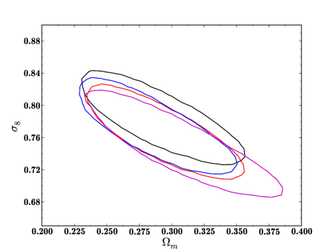
We perform the same analysis as on the baseline cosmological sample (SZ+BAO+BBN), but employing a different computation of the completeness function using the Monte Carlo method described in Sect. 3. Figure 9 shows the change in the 2D likelihoods when this alternative approach is adopted. The Monte Carlo estimation (in purple), being close to the analytic one, gives constraints that are similar, but enlarge the contour along the ($\Omega_{\mathrm{m}},\sigma_{8}$) degeneracy.

5.3 Robustness to cluster modelling

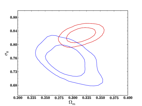
A key ingredient in the modelling of the number counts is the mass function. Our main results adopt the Tinker et al. mass function as the reference model. We compare these to results from the Watson et al.  mass function to evaluate the impact of uncertainty in predictions for the abundance of the most massive and extreme clusters. Figure 8 shows the 95% contours when adopting the different mass functions. The main effect is to change the orientation of the degeneracy between $\Omega_{\mathrm{m}}$ and $\sigma_{8}$, moving the best-fit values by less than $1\thinspace\sigma$.

We also relax the assumption of standard evolution of the scalings with redshift by allowing $\beta$ to vary with a Gaussian prior taken from Planck Collaboration X (2011), $\beta=0.66\pm 0.5$. Once again, the contours move along the $\sigma_{8}$–$\Omega_{\mathrm{m}}$ degeneracy direction (shown in blue in Fig. 8).

As shown in Appendix A, the estimation of the mass bias is not trivial and there is a large scatter amongst simulations. The red and purple contours compare the different constraints when fixing the mass bias to 0.8 and when allowing it to vary uniformly in the range $[0.7,1.0]$ respectively. Modelling of the cluster observable–mass relation is clearly the limiting factor in our analysis.

6 Discussion

Our main result is the constraint in the $(\Omega_{\mathrm{m}},\sigma_{8})$ plane for the standard $\Lambda$CDM model imposed by the SZ counts, which we have shown is robust to the details of our modelling. We now compare this result first to constraints from other cluster samples, and then to the constraints from the Planck analysis of the sky-map of the Compton $y$-parameter (Planck Collaboration XXI, 2014) and of the primary CMB temperature anisotropies (Planck Collaboration XVI, 2014).

6.1 Comparison with other cluster constraints

We restrict our comparison to some recent analyses exploiting a range of observational techniques to obtain cluster samples and mass calibrations.

Benson et al. (2013) used 18 galaxy clusters in the first $178\thinspace{\mathrm{deg}}^{2}$ of the SPT survey to find $\sigma_{8}(\Omega_{\mathrm{m}}/0.25)^{0.3}=0.785\pm 0.037$ for a spatially-flat model. They break the degeneracy between $\sigma_{8}$ and $\Omega_{\mathrm{m}}$ by incorporating primary CMB constraints, deducing that $\sigma_{8}=0.795\pm 0.016$ and $\Omega_{\mathrm{m}}=0.255\pm 0.016$. In addition, they find that the dark energy equation of state is constrained to $w=-1.09\pm 0.36$, using just their cluster sample along with the same HST and BBN constraints used here. Subsequently, Reichardt et al. (2013) reported a much larger cluster sample and used this to improve on the statistical uncertainties on the cosmological parameters (see Table 3). Hasselfield et al. (2013) use a sample of 15 high S/N clusters from ACT, in combination with primary CMB data, to find $\sigma_{8}=0.786\pm 0.013$ and $\Omega_{\mathrm{m}}=0.250\pm 0.012$ when assuming a scaling law derived from the universal pressure profile.

Figure 10: Comparison of constraints (68% confidence interval) on $\sigma_{8}(\Omega_{\mathrm{m}}/0.27)^{0.3}$ from different experiments of large–scale structure (LSS), clusters, and CMB. The solid line ACT point assumes the same universal pressure profile as this work. Probes marked with an asterisk have an original power of $\Omega_{\mathrm{m}}$ different from 0.3. See text and Table 3 for more details.

Table 3: Constraints from clusters on $\sigma_{8}(\Omega_{\mathrm{m}}/0.27)^{0.3}$.

Experiment      CPPP^a      MaxBCG^b      ACT^c      SPT      Planck SZ

Reference      Vikhlinin et al.      Rozo et al.      Hasselfield et al.      Reichardt et al.      This work

     (2009b)      (2010)      (2013)      (2013)

Number of clusters      49+37      $$\sim$$13000      15      100      189

Redshift range       and                        

Median mass ()      2.5      1.5      3.2      3.3      6.0

Probe                              

S/N cut      5      ()      5      5      7

Scaling      –,      –      several      –,      –

                             

^aThe degeneracy is $$\sigma_{8}(\Omega_{\mathrm{m}}/0.27)^{0.47}$$.

^bThe degeneracy is $$\sigma_{8}(\Omega_{\mathrm{m}}/0.27)^{0.41}$$.

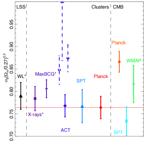
^cFor ACT we choose the results assuming the scaling law derived from the universal pressure profile in this table (constraints using other scaling relations are shown in Fig. 10).

Strong constraints on cosmological parameters have been inferred from X-ray and optical richness selected samples. Vikhlinin et al. (2009b) used a sample of 86 well-studied X-ray clusters, split into low- and high-redshift bins, to conclude that $\Omega_{\Lambda}>0$ with a significance about $5\thinspace\sigma$ and that $w=-1.14\pm 0.21$. Rozo et al. (2010) used the approximately $10^{4}$ clusters in the Sloan Digital Sky Survey (SDSS) MaxBCG cluster sample, which are detected using a colour–magnitude technique and characterized by optical richness. They found that $\sigma_{8}(\Omega_{\mathrm{m}}/0.25)^{0.41}=0.832\pm 0.033$. The fact that this uncertainty is similar to those quoted above for much smaller cluster samples signifies, once again, that cluster cosmology constraints are now limited by modelling, rather than statistical, uncertainties.

Table 3 and Fig. 10 show some current constraints on the combination $\sigma_{8}(\Omega_{\mathrm{m}}/0.27)^{0.3}$, which is the main degeneracy line in cluster constraints. This comparison is only meant to be indicative, as a more quantitative comparison would require full consideration of modelling details which is beyond the scope of this work. Cosmic shear (Kilbinger et al., 2013), X-rays (Vikhlinin et al., 2009b), and MaxBCG (Rozo et al., 2010) each have a different slope in $\Omega_{\mathrm{m}}$, being 0.6, 0.47, and 0.41, respectively (instead of 0.3), as they are probing different redshift ranges. We have rescaled when necessary the best value and errors to quote numbers with a pivot $\Omega_{\mathrm{m}}=0.27$. Hasselfield et al. (2013) have derived ‘cluster-only’ constraints from ACT by adopting several different scaling laws, shown in blue and dashed blue in Fig. 10. The constraint assuming the universal pressure profile is highlighted as the solid symbol and error bar. For SPT we show the ‘cluster-only’ constraints from Reichardt et al. (2013). For our own analysis we show our baseline result for SZ+BAO+BBN with a prior on $(1-b)$ distributed uniformly in $[0.7,1]$. The figure thus demonstrates good agreement amongst all cluster observations, whether in optical, X-rays, or SZ. Table 3 compares the different data and assumptions of the different cluster-related publications.

6.2 Consistency with the Planck y-map

In a companion paper (Planck Collaboration XXI, 2014), we performed an analysis of the SZ angular power spectrum derived from the Planck $y$-map obtained with a dedicated component-separation technique. For the first time, the power spectrum has been measured at intermediate scales ($50\leq\ell\leq 1000$). The same modelling as in Sect. 2 and Taburet et al. (2009, 2010) has been used to derive best-fit values of $\Omega_{\mathrm{m}}$ and $\sigma_{8}$, assuming the universal pressure profile (Arnaud et al., 2010), a bias $1-b=0.8$, and the best-fit values for other cosmological parameters from Planck Collaboration XVI (2014). The best model obtained, shown in Fig. 7 as the dashed line, demonstrates the consistency between the PSZ number counts and the signal observed in the $y$-map.

6.3 Comparison with Planck primary CMB constraints

We now compare the PSZ cluster constraints to those from the analysis of the primary CMB temperature anisotropies given in Planck Collaboration XVI (2014) (see Footnote 6). In that analysis $\sigma_{8}$ is derived from the standard six $\Lambda$CDM parameters.

The Planck primary CMB constraints, in the $(\Omega_{\mathrm{m}},\sigma_{8})$ plane, differ significantly from our own, in particular through favouring a higher value of $\sigma_{8}$, (see Fig. 11). For $(1-b)=0.8$, this leads to a factor of $∼2$ larger number of predicted clusters than is actually observed (see Fig. 7). There is therefore some tension between the results from the Planck CMB analysis and the current cluster analysis. Figure 10 illustrates this with a comparison of three analyses of primary CMB data alone (Planck Collaboration XVI, 2014; Story et al., 2012; Hinshaw et al., 2013) and cluster constraints in terms of $\sigma_{8}(\Omega_{\mathrm{m}}/0.27)^{0.3}$.

Figure 11: 2D $\Omega_{\mathrm{m}}$–$\sigma_{8}$ likelihood contours for the analysis with Planck CMB only (red); Planck SZ + BAO + BBN (blue) with $(1-b)$ in $[0.7,1]$.

It is possible that the tension results from a combination of some residual systematics with a substantial statistical fluctuation. Enough tests and comparisons have been made on the Planck data sets that it is plausible that at least one discrepancy at the two or three sigma level will arise by chance. Nevertheless, it is worth considering the implications if the discrepancy is real.

As we have noted, the modelling of the cluster gas physics is the most important uncertainty in our analysis, in particular through its influence on the mass bias $(1-b)$. While we have argued for a preferred value of $(1-b)\simeq 0.8$ based on comparison of our $Y_{500}$–$M_{500}$ relation to those derived from a number of different numerical simulations, and we suggest a plausible range of $(1-b)$ from 0.7 to 1, a significantly lower value would substantially alleviate the tension between CMB and SZ constraints. We have undertaken a joint analysis using the CMB likelihood presented in Planck Collaboration XV (2014) and the cluster likelihood presented in the present paper, sampling $(1-b)$ in the range $[0.1,1.5]$. This results in a ‘measurement’ of $(1-b)=0.59\pm 0.05$. We show in Fig 7 the SZ cluster counts predicted by the Planck’s best-fit primary CMB model for $(1-b)=0.59$. Clearly, this substantial reduction in $(1-b)$ is enough to reconcile our observed SZ cluster counts with Planck’s best fit primary CMB parameters.

Such a large bias is difficult to reconcile with numerical simulations, and cluster masses estimated from X-rays and from weak lensing do not typically show such large offsets (see Appendix A). Systematic discrepancies in the relevant scaling relations have, however, been identified and studied in stacking analyses of X-ray, SZ, and lensing data for the very large MaxBCG cluster sample, e.g., Planck Collaboration XII (2011), Biesiadzinski et al. (2012), Draper et al. (2012), Rozo et al. (2012a), and Sehgal et al. (2013), suggesting that the issue is not yet fully settled from an observational point of view. The uncertainty reflects the inherent biases of the different mass estimates. Systematic effects arising from instrument calibration constitute a further source of uncertainty — in X-ray mass determinations, temperature estimates represent the main source of systematic uncertainty in mass, as the mass scales roughly with $T^{3/2}$. Other biases in the determination of mass–observable scaling relations come from the object selection process itself (e.g., Mantz et al., 2010; Allen et al., 2011; Angulo et al., 2012). This may be less of a concern for SZ selected samples because of the expected small scatter between the measured quantity and the mass. An improbable conspiracy of all sources of bias seems required to lead to a sufficiently-low effective value of $(1-b)$ to reconcile the SZ and CMB constraints. This possibility needs to be carefully examined with probes based on a variety of physical quantities and derived from a wide range of types of observation, including masses, baryon and gas fractions, etc.

A different mass function may also help reduce the tension. Mass functions are calibrated against numerical simulations that may still suffer from volume effects for the largest haloes, as shown in the difference between the Tinker et al. (2008) and Watson et al. (2013) mass functions. This does not seem sufficient, however, given the results presented in Fig. 8.

One might instead ask whether the Planck data analysis could somehow have missed a non-negligible fraction of the total number of clusters currently predicted to have $\mathrm{S/N}>7$, resulting in a lower observed number count distribution. This is linked to a possible underestimate of the true dispersion about the $Y_{500}$–$Y_{\mathrm{X}}$ relation at a given $M_{\mathrm{500}}$. It would be necessary for Planck to have missed $\sim$40 percent of the clusters with predicted SZ $\mathrm{S/N}>7$ in order for the SZ and CMB number count curves in Fig. 7 to be in agreement. Increasing the dispersion about the $Y_{500}$–$M_{\mathrm{500}}$ relation and allowing it to correlate strongly with the scatter in X-ray properties (in particular, $Y_{\mathrm{X}}$) would raise the possibility that our calibration procedures (which are based on X-ray and SZ selected clusters assuming the scatter in $Y$ and $Y_{\mathrm{x}}$ at fixed $M_{\mathrm{500}}$ to be small and to be uncorrelated with cluster dynamical state) might produce a relation which is biased high. A sufficiently-large effect seems, however, to require a level of scatter and a degree of correlation with cluster structure which are inconsistent with the predictions of current hydrodynamical simulations (see the discussion in Appendix A).

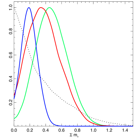
Alternatively, the discrepancy may reflect a need to extend the minimal $\Lambda$CDM model in which the $\sigma_{8}$ constraints are derived from the primary CMB analysis. Any extension would need to modify the power spectrum on the scales probed by clusters, while leaving the scales probed by primary CMB observations unaffected. The inclusion of neutrino masses, quantified by their sum over all families, $\sum m_{\nu}$, can achieve this (see Marulli et al. 2011 and Burenin 2013 for reviews of how cosmological observations can be affected by the inclusion of neutrino masses). The SPT collaboration (Hou et al., 2014) recently considered such a possibility to mitigate their tension with WMAP-7 primary CMB data. There is an upper limit of $\sum m_{\nu}<0.93\thinspace$eV from the Planck primary CMB data alone. If we combine the Planck CMB (Planck+WP) likelihood and the cluster count data using a fixed value $(1-b)=0.8$, then we find a $2.8\thinspace\sigma$ preference for the inclusion of neutrino masses with $\sum m_{\nu}=(0.53\pm 0.19)\thinspace$eV, as shown in Fig. 12. If, on the other hand, we adopt a more conservative point of view and allow $(1-b)$ to vary between 0.7 and 1.0, this preference drops to $1.9\sigma$ with $\sum m_{\nu}=(0.40\pm 0.21)\thinspace$eV. Adding BAO data to the compilation lowers the value of the required mass but increases the significance, yielding $\sum m_{\nu}=(0.20\pm 0.09)\thinspace$eV, due to a breaking of the degeneracy between $H_{0}$ and $\sum m_{\nu}$.

Figure 12: Marginalized posterior distribution for $\sum m_{\nu}$ from: Planck CMB data alone (black dotted line); Planck CMB + SZ with $1-b$ in $[0.7,1]$ (red); Planck CMB + SZ + BAO with $1-b$ in $[0.7,1]$ (blue); and Planck CMB + SZ with $1-b=0.8$ (green).

As these results depend on the value and allowed range of $(1-b)$, better understanding of the scaling relation is the key to further investigation. This provides strong motivation for further study of the relationship between $Y$ and $M$. Over the past few years we have moved into an era where systematic uncertainties dominate to an increasing extent over statistical uncertainties. Observed mass estimates using different methods are of improving quality; for instance, X-ray mass proxies can be measured to better than 10% precision (e.g., Vikhlinin et al., 2006; Arnaud et al., 2007). In this context, systematic calibration uncertainties are playing an increasingly important role when using the cluster population to constrain cosmology.

7 Summary

We have used a sample of nearly 200 clusters from the PSZ, along with the corresponding selection function, to place strong constraints in the $(\Omega_{\mathrm{m}},\sigma_{8})$ plane. We have carried out a series of tests to verify the robustness of our constraints, varying the observed sample choice, the estimation method for the selection function, and the theoretical methodology, and have found that our results are not altered significantly by those changes.

The relation between the mass and the integrated SZ signal plays a major role in the computation of the expected number counts. Uncertainties in cosmological constraints from clusters are no longer dominated by small number statistics, but by the gas physics and sample selection biases. Uncertainties in the $Y$–$M$ relation include contributions from X-ray instrument calibration, X-ray temperature measurements, inhomogeneities in cluster density and temperature profiles, and selection effects. Considering several ingredients of the gas physics of clusters, numerical simulations predict scaling relations with 30% scatter in amplitude (at a fiducial mass of $6\times 10^{14}\mathrm{M}_{\odot}$), and suggest a mass bias between the true mass and the estimated mass of $(1-b)=0.8^{+0.2}_{-0.1}$. Adopting the central value we found constraints on $\Omega_{\mathrm{m}}$ and $\sigma_{8}$ that are in good agreement with previous measurements using clusters of galaxies.

Comparing our results with Planck primary CMB constraints within the $\Lambda$CDM cosmology reveals some tension. This can be alleviated by permitting a large mass bias ($1-b\simeq 0.60$), which is however significantly larger than expected. Alternatively, the tension may indicate a need for an extension of the base $\Lambda$CDM model that modifies its power spectrum shape. For example the inclusion of non-zero neutrino masses helps in reconciling the primary CMB and cluster constraints, a fit to Planck CMB + SZ + BAO yielding $\sum m_{\nu}=(0.20\pm 0.09)\thinspace$eV.

Cosmological parameter determination using clusters is currently limited by the knowledge of the observable–mass relations. In the future our goal is to increase the number of dedicated follow-up programmes to obtain better estimates of the mass proxy and redshift for most of the S/N $>5$ Planck clusters. This will allow for improved determination of the scaling laws and the mass bias, increase the number of clusters that can be used, and allow us to investigate an extended cosmological parameter space.

Appendix A Calibration of the $Y_{500}$–$M_{\mathrm{500}}$ relation

A cluster catalogue is a list of positions and measurements of observable physical quantities. Its scientific utility depends largely on our ability to link the observed quantities to the underlying mass, in other words, to define an observable proxy for the mass. Planck detects clusters through the SZ effect. This effect is currently the subject of much study in the cluster community, chiefly because numerical simulations indicate that the spherically-integrated SZ measurement is correlated particularly tightly with the underlying mass. In other words, this measurement potentially represents a particularly valuable mass proxy.

To establish a mass proxy, one obviously needs an accurate measurement both of the total mass and of the observable quantity in question. However, even with highly accurate measurements, the correlation between the observable quantity and the mass is susceptible to bias and dispersion, and both of these effects need to be taken into account when using cluster catalogues for scientific applications.

The aim of this Appendix is to define a baseline relation between the measured SZ flux, $Y_{500}$, and the total mass $M_{\mathrm{500}}$. The latter quantity is not directly measurable. On an individual cluster basis, it can be inferred from dynamical analysis of galaxies, from X-ray analysis assuming hydrostatic equilibrium (HE), or from gravitational lensing observations. However, it is important to note that all observed mass estimates include inherent biases. For instance, numerical simulations suggest that HE mass measurements are likely to underestimate the true mass by $10$–$15$ percent due to neglect of bulk motions and turbulence in the intra-cluster medium (ICM, e.g., Nagai et al. 2007; Piffaretti & Valdarnini 2008; Meneghetti et al. 2010), an effect that is commonly referred to in the literature as the ‘hydrostatic mass bias’. Similarly, simulations indicate that weak lensing mass measurements may underestimate the mass by 5 to 10 percent, owing to projection effects or the use of inappropriate mass models (e.g., Becker & Kravtsov 2011). Instrument calibration systematic effects constitute a further source of error. For X-ray mass determinations, temperature estimates represent the main source of systematic uncertainty, as the mass at a given density contrast scales roughly with $T^{3/2}$. Other biases in the determination of mass–observable scaling relations come from the object selection process itself (e.g., Allen et al. 2011; Angulo et al. 2012). A classic example is the Malmquist bias, where bright objects near the flux limit are preferentially detected. This effect is amplified by Eddington bias, the mass function dictating that many more low-mass objects are detected compared to high-mass objects. Both of these biases depend critically on the distribution of objects in mass and redshift, and on the dispersion in the relation between the mass and the observable used for sample selection. This is less of a concern for SZ selected samples than for X-ray selected samples, the SZ signal having much less scatter at a given mass than the X-ray luminosity. However for precise studies it should still be taken into account.

On the theoretical side, numerous $Y_{500}$–$M_{\mathrm{500}}$ relations have been derived from simulated data, as discussed below. The obvious advantage of using simulated data is that the relation between the SZ signal and the true mass can be obtained, because the ‘real’ value of all physical quantities can be measured. The disadvantage is that the ‘real’ values of measurable physical quantities depend strongly on the phenomenological models used to describe the different non-gravitational processes at work in the ICM.

Nevertheless, the magnitude of the bias between observed and true quantities can only be assessed by comparing multi-wavelength observations of a well-controlled cluster sample to numerical simulations. Thus, ideally, we would have full follow-up of a complete Planck cluster sample. For large samples, however, full follow-up is costly and time consuming. This has led to the widespread use of mass estimates obtained from mass–proxy relations. These relations are generally calibrated from individual deep observations of a subset of the sample in question (e.g., Vikhlinin et al. 2009a), or from deep observations of objects from an external dataset (e.g., the use of the REXCESS relations in Planck Collaboration XI 2011).

For the present paper, we will rely on mass estimates from a mass–proxy relation. In this context, the $M_{\mathrm{500}}$–$Y_{\mathrm{X}}$ relation is clearly the best to use. $Y_{\mathrm{X}}$, proposed by Kravtsov et al. (2006), is defined as the product of $M_{\mathrm{g},500}$, the gas mass within $R_{500}$, and $T_{\mathrm{X}}$, the spectroscopic temperature measured in the $[0.15$–$0.75]\leavevmode\nobreak\ R_{500}$ aperture. In the simulations performed by Kravtsov et al. (2006), $Y_{\mathrm{X}}$ was extremely tightly correlated with the true cluster mass, with a logarithmic dispersion of only $8$ percent. Observations using masses derived from X-ray hydrostatic analysis indicate that $Y_{\mathrm{X}}$ does indeed appear to have a low dispersion (Arnaud et al. 2007; Vikhlinin et al. 2009a). Furthermore, the local $M_{\mathrm{500}}$–$Y_{\mathrm{X}}$ relation for X-ray selected relaxed clusters has been calibrated to high statistical precision (Arnaud et al. 2010; Vikhlinin et al. 2009a), with excellent agreement achieved between various observations (see e.g., Arnaud et al. 2007). Since simulations suggest that the $Y_{500}$–$M_{\mathrm{500}}$ relation is independent of dynamical state, calibrating the $Y_{500}$–$M_{\mathrm{500}}$ relation via a low-scatter mass proxy, itself calibrated on clusters for which the HE bias is expected to be minimal, is a better approach than using HE mass estimates for the full sample, since the latter can be highly biased for very unrelaxed objects.

Table 4: Parameters for the $Y_{500}$–$M_{\mathrm{500}}$ relation, expressed as $E^{-2/3}(z)\left[D_{\mathrm{A}}^{2}Y_{500}/10^{-4}{\mathrm{Mpc^{2}}}\right]=10^{A}\left[M_{\mathrm{500}}/6\times 10^{14}\mathrm{M}_{\odot}\right]^{\alpha}$.

Sample      $$N_{\mathrm{c}}$$      MB      Mass                   int       raw      Section

XMM-ESZ PEPXI      62      N                              …      A.2.1

Cosmo sample      71      N                                    A.2.1

Cosmo sample      71      Y                                    A.2.2

XMM-ESZ      62      Y                                    A.2.3

S/N            Y                                    A.2.3

Cosmo sub-sample A      10      Y                        …            A.3.2

Cosmo sub-sample B      58      Y                                    A.3.2

We approach the determination of the $Y_{500}$–$M_{\mathrm{500}}$ relation in two steps. We first calibrate the $Y_{500}$–proxy relation. This is combined with the X-ray calibrated relation, between the proxy and $M_{\mathrm{500}}$, to define an observation-based $Y_{500}$–$M_{\mathrm{500}}$ relation. In the second step, we assess possible biases in the relation by directly comparing the observation-based relation with that from simulations. This approach, rather than directly assessing the HE mass bias, allows us to avoid complications linked to the strong dependence of the HE bias on cluster dynamical state, and thus on the cluster sample (real or simulated). The final output from this procedure is a relation between $Y_{500}$ and $M_{\mathrm{500}}$, with a full accounting of the different statistical and systematic uncertainties that go into its derivation, including bias.

In the following, all relations are fit with a power law in log-space using the orthogonal BCES method (Akritas & Bershady 1996), which takes into account the uncertainties in both variables and the intrinsic scatter. All dispersions are given in log₁₀.

A.1 Baseline mass–proxy relation

As a baseline, we use the relation between $Y_{\mathrm{X}}$ and the X-ray hydrostatic mass $M_{\mathrm{500}}^{\mathrm{HE}}$ established for 20 local relaxed clusters by Arnaud et al. (2010):

$$E^{-2/3}(z)\left[\frac{Y_{\mathrm{X}}}{2\times 10^{14}\mathrm{M}_{\odot}\thinspace\mathrm{keV}}\right]\hskip 85.35826pt$$ (14)

$$\hskip 56.9055pt=10^{0.376\pm 0.018}\left[\frac{M_{\mathrm{500}}^{\mathrm{HE}}}{6\times 10^{14}\mathrm{M}_{\odot}}\right]^{1.78\pm 0.06},$$

assuming standard evolution, and where the uncertainties are statistical only. For easier comparison with the $Y_{500}$–$M_{\mathrm{500}}$ relation given below, the normalization for $Y_{\mathrm{X}}$ expressed in $10^{-4}\thinspace{\mathrm{Mpc}}^{2}$ is $10^{-0.171\pm 0.018}$. The HE mass is expected to be a biased estimator of the true mass,

$$M_{\mathrm{500}}^{\mathrm{HE}}=(1-b)\thinspace M_{\mathrm{500}}\thinspace,$$ (15)

where all of the possible observational biases discussed above (departure from HE, absolute instrument calibration, temperature inhomogeneities, residual selection bias) have been subsumed into the bias factor $(1-b)$. The form of the $Y_{\mathrm{X}}$–$M_{\mathrm{500}}$ relation is thus

$$E^{-2/3}(z)Y_{\mathrm{X}}=10^{A\pm\sigma_{\mathrm{A}}}\thinspace\left[(1-b)\thinspace M_{\mathrm{500}}\right]^{\alpha\pm\sigma_{\mathrm{\alpha}}}\thinspace,$$ (16)

where $\sigma_{\mathrm{A}}$ and $\sigma_{\mathrm{\alpha}}$ are the statistical uncertainties on the normalization and slope and $b$ is the bias between the true mass and the observed mass used to calibrate the relation. The bias is a poorly-known stochastic variable with substantial variation expected between clusters. In our case, $b$ represents the mean bias between the observed mass and the true mass.

The mass proxy $M_{\mathrm{500}}^{Y_{\mathrm{X}}}$ is defined from the best-fit $Y_{\mathrm{X}}$–$M_{\mathrm{500}}^{\mathrm{HE}}$ relation

$$E^{-2/3}(z)Y_{\mathrm{X}}=10^{A}\thinspace\left[M_{\mathrm{500}}^{Y_{\mathrm{X}}}\right]^{\alpha}\thinspace.$$ (17)

For any cluster, $M_{\mathrm{500}}^{Y_{\mathrm{X}}}$, together with the corresponding $Y_{\mathrm{X}}$ and $R_{500}^{Y_{\mathrm{X}}}$, can be estimated iteratively about this relation from the observed temperature and gas mass profile, as described in Kravtsov et al. (2006). The calibration of the $Y_{\mathrm{X}}$–$M_{\mathrm{500}}$ relation is equivalent to a calibration of the $M_{\mathrm{500}}^{Y_{\mathrm{X}}}$–$M_{\mathrm{500}}$ relation, which relates the mass proxy, $M_{\mathrm{500}}^{Y_{\mathrm{X}}}$, to the mass via

$$M_{\mathrm{500}}^{Y_{\mathrm{X}}}=10^{\pm\sigma_{\mathrm{A}}/\alpha}\thinspace\left[(1-b)\thinspace M_{\mathrm{500}}\right]^{1\pm\sigma_{\mathrm{\alpha}}/\alpha}\thinspace.$$ (18)

In addition to the bias factor, there are statistical uncertainties on the slope and normalization of the relation, as well as intrinsic scatter around the relation, linked to the corresponding statistical uncertainties and scatter of the $Y_{\mathrm{X}}$–$M_{\mathrm{500}}^{\mathrm{HE}}$ relation.

A.2 Relation between $Y_{500}$ and $M_{\mathrm{500}}^{Y_{\mathrm{X}}}$

A.2.1 Best-fit relation

We first investigate the relationship between $Y_{500}$ and $M_{\mathrm{500}}^{Y_{\mathrm{X}}}$, the mass estimated iteratively from Eq. 17, with parameters given by the best-fit Arnaud et al. (2010) relation (Eq. 14). Full X-ray follow-up of the Planck SZ cosmological cluster sample is not yet available. Our baseline sample is thus a subset of 71 detections from the Planck cosmological cluster sample, detected at S/N $>7$, for which good quality XMM-Newton observations are available. The sample consists of data from our previous archival study of the Planck Early SZ (ESZ) clusters (Planck Collaboration XI 2011), of Planck-detected LoCuSS clusters presented by Planck Collaboration Int. III (2013), and from the XMM-Newton validation programme (Planck Collaboration IX 2011; Planck Collaboration Int. I 2012; Planck Collaboration Int. IV 2013). The corresponding sub-samples include 58, 4, and 9 clusters, respectively. The X-ray data were re-analysed in order to have a homogeneous data set; measurement differences are negligible with respect to previously-published values. Uncertainties on $Y_{\mathrm{X}}$, $R_{500}^{Y_{\mathrm{X}}}$, and $M_{\mathrm{500}}^{Y_{\mathrm{X}}}$ include those due to statistical errors on the X-ray temperature and the gas mass profile.

The SZ signal is estimated within a sphere of radius $R_{500}^{Y_{\mathrm{X}}}$ centred on the position of the X-ray peak, as detailed in e.g., Planck Collaboration XI (2011). The re-extraction procedure uses matched multi-filters (MMF) and assumes that the ICM pressure follows the universal profile shape derived by Arnaud et al. (2010) from the combination of the REXCESS sample with simulations. The extraction is undertaken on the 15.5 month Planck survey data set, and so statistical precision on the SZ signal is improved with respect to previously-published values. The uncertainty on $Y_{500}$ includes statistical uncertainties on the SZ signal derived from the MMF, plus the statistical uncertainty on the aperture $R_{500}^{Y_{\mathrm{X}}}$. The latter uncertainty is negligible compared to the statistical error on the SZ signal. The resulting relation for these 71 clusters from the cosmological sample is

$$E^{-2/3}(z)\left[\frac{D_{\mathrm{A}}^{2}\thinspace Y_{500}}{\mathrm{10^{-4}\thinspace Mpc^{2}}}\right]\hskip 85.35826pt$$ (19)

$$\hskip 56.9055pt=10^{-0.175\pm 0.011}\left[\frac{M_{\mathrm{500}}^{Y_{\mathrm{X}}}}{6\times 10^{14}\mathrm{M}_{\odot}}\right]^{1.77\pm 0.06}.$$

This agrees within $1\sigma$ with the results from the sample of 62 clusters from the ESZ sample with archival XMM-Newton data published in Planck Collaboration XI (2011). The slope and normalization are determined at slightly higher precision, due to the better quality SZ data. The derived intrinsic scatter (Table 4) is significantly smaller. This is a consequence of: a more robust treatment of statistical uncertainties; propagation of gas mass profile uncertainties in the $Y_{\mathrm{X}}$ error budget; and, to a lesser extent, the propagation of $R_{500}^{Y_{\mathrm{X}}}$ uncertainties to $Y_{500}$ estimates.

A.2.2 Effects of Malmquist bias

The fitted parameters are potentially subject to selection effects such as Malmquist bias, owing to part of the sample lying close to the selection cut. For the present sample, we use an approach adapted from that described in Vikhlinin et al. (2009a) and Pratt et al. (2009), where each data point is rescaled by the mean bias for its flux, and the relation refitted using the rescaled points. The method is described in more detail in Paper 1. For the baseline cosmological sample of 71 systems, the bias-corrected $Y_{500}$–$M_{\mathrm{500}}^{Y_{\mathrm{X}}}$ relation is

$$E^{-2/3}(z)\left[\frac{D_{\mathrm{A}}^{2}\thinspace Y_{500}}{\mathrm{10^{-4}\thinspace Mpc^{2}}}\right]\hskip 85.35826pt$$ (20)

$$\hskip 56.9055pt=10^{-0.19\pm 0.01}\left[\frac{M_{\mathrm{500}}^{Y_{\mathrm{X}}}}{6\times 10^{14}\mathrm{M}_{\odot}}\right]^{1.79\pm 0.06}\thinspace.$$

The best-fit relation, together with Malmquist bias corrected data points, is plotted in Fig. 13.

Figure 13: Best scaling relation between $Y_{500}$ and $M_{\mathrm{500}}$, and the data points utilized after correction of the Malmquist bias

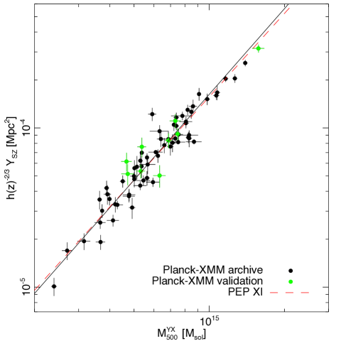
The correction decreases the effective $Y_{500}$ values at a given mass, an effect larger for clusters closer to the S/N threshold. The net effect is small, a roughly $1\thinspace\sigma$ decrease of the normalization and a slight steepening of the power-law slope (Table 4).

A.2.3 Stability of slope and normalization

The slope and normalization of this relation are robust to the choice of sample (Table 4). We compared our results to those obtained from:

• An extended sample of 78 clusters with $S/N>7$ (71 in common with the baseline sample). This is built from all objects falling in the 84% sky mask used to define the SZ catalogue Planck Collaboration XXIX (2014), and for which XMM-Newton data have been published by the Planck Collaboration (Planck Collaboration IX 2011; Planck Collaboration XI 2011; Planck Collaboration Int. I 2012; Planck Collaboration Int. III 2013; Planck Collaboration Int. IV 2013).

• The original 62 clusters from the ESZ sample published in Planck Collaboration XI (2011), with updated SZ signal measurements obtained from 15.5 month Planck data (62 in common with the baseline sample). These objects are all known from X-ray surveys and all lie at $z<0.5$. We use them to test fit robustness to the inclusion of non-X-ray selected, higher-redshift systems.

As indicated in Table 4, there is agreement within $1\thinspace\sigma$ between the various samples. The results are also in agreement with the relation obtained from a simple combination of the $Y_{500}$–$Y_{\mathrm{X}}$ relation (discussed in Paper 1) and the $Y_{\mathrm{X}}$–$M_{\mathrm{500}}^{\mathrm{HE}}$ relation (Eq. 14 above).

A.3 The observation-based $Y_{500}$–$M_{\mathrm{500}}$ relation

A.3.1 Combination of the $Y_{500}$–$M_{\mathrm{500}}^{Y_{\mathrm{X}}}$ and the $M_{\mathrm{500}}^{Y_{\mathrm{X}}}$–$M_{\mathrm{500}}$ relations

We now combine Eq. 20 with the $M_{\mathrm{500}}^{Y_{\mathrm{X}}}$–$M_{\mathrm{500}}$ relation. This will not change the best-fit parameters, but will increase their uncertainties. As the determinations of the two relations are independent, we added quadratically the uncertainties in the best-fit parameters of the $Y_{500}$–$M_{\mathrm{500}}^{Y_{\mathrm{X}}}$ (Eq. 19) and $M_{\mathrm{500}}^{Y_{\mathrm{X}}}$–$M_{\mathrm{500}}$ (Eq. 18, with values from Eq. 14) relations. Our best-fit $Y_{500}$–$M_{\mathrm{500}}$ relation is then

$$E^{-2/3}(z)\left[\frac{D_{\mathrm{A}}^{2}\thinspace Y_{500}}{\mathrm{10^{-4}\thinspace Mpc^{2}}}\right]\hskip 71.13188pt$$ (21)

$$\hskip 56.9055pt=10^{-0.19\pm 0.02}\left(\frac{(1-b)\thinspace M_{\mathrm{500}}}{6\times 10^{14}\mathrm{M}_{\odot}}\right)^{1.79\pm 0.08}.$$

Thus inclusion of the statistical uncertainty in the $M_{\mathrm{500}}^{Y_{\mathrm{X}}}$–$M_{\mathrm{500}}^{\mathrm{HE}}$ relation doubles the uncertainty on the normalization and increases the uncertainty on the slope by $40\%$. Note that we have implicitly assumed here that the scatter around the two relations is uncorrelated.

A.3.2 Effect of use of an external dataset

The above results assume a mass estimated from the baseline $Y_{\mathrm{X}}$–$M_{500}$ relation, derived by Arnaud et al. (2010) from an external dataset of 20 relaxed clusters (Eq 14). How does this relation compare to the individual hydrostatic X-ray masses of the Planck cosmological cluster sample? Of the 71 clusters in the baseline sample:

• 58 objects have temperature profile information extending to various fractions of $R_{500}$, of which

• 10 cool-core objects have temperature profiles measurements at least out to $R_{500}$.

Thus, while spatially-resolved temperature profiles are available for 58 of the 71 clusters with XMM-Newton observations, we must be careful in interpretation of these data. The Arnaud et al. relation was derived from a carefully chosen data set consisting of relaxed, cool-core objects having well-constrained temperature profiles out to around $R_{500}$, i.e., the type of object for which it makes sense to undertake a hydrostatic mass analysis. Many clusters of the Planck sample are merging systems for which such an analysis would give results that are difficult to interpret. In addition, few of the Planck sample have spatially-resolved temperature profiles out to $R_{500}$. However, as given in Table 4, the best-fit $Y_{\mathrm{X}}$–$M_{\mathrm{500}}^{\mathrm{HE}}$ relation for the 10 cool-core clusters that are detected to $R_{500}$ agrees with Eq. 21 within $1\thinspace\sigma$. Moreover, the relation for the 58 Planck clusters with HE mass estimates, derived regardless of dynamical state and radial detection extent, also agrees within $1\thinspace\sigma$ (albeit with greatly increased scatter). We are thus confident that the masses estimated from an externally-calibrated $Y_{\mathrm{X}}$–$M_{\mathrm{500}}^{\mathrm{HE}}$ relation are applicable to the present data set.

Figure 14: Left: comparison of $Y_{500}$–$M_{\mathrm{500}}$ relations from 12 simulations undertaken by six different groups with the updated observational $Y_{500}$–$M_{\mathrm{500}}^{\mathrm{HE}}$ result from Planck, Eq. 21. Right: ratio of each simulated $Y_{500}$–$M_{\mathrm{500}}$ relation relative to Eq. 21. The different scaling laws are taken from Kay et al. (2012), Battaglia et al. (2012), Yang et al. (2010), Sehgal et al. (2010), Krause et al. (2012), Nagai (2006), Sembolini et al. (2013) and Planck Collaboration XI (2011).

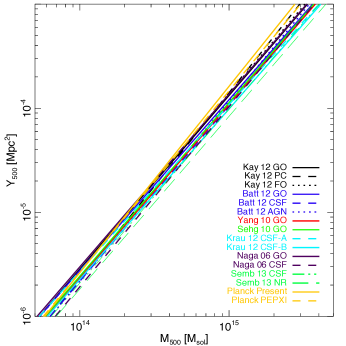
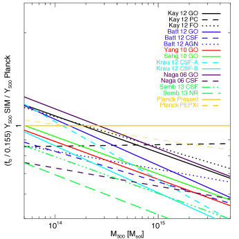
A.3.3 Dispersion about the observed relations

A key issue is the dispersion around the mean relation. We first estimate the intrinsic scatter of the $Y_{500}$–$M_{\mathrm{500}}^{\mathrm{HE}}$ relation by combining the intrinsic scatter of the $Y_{500}$–$M_{\mathrm{500}}^{Y_{\mathrm{X}}}$ relation and that of the $M_{\mathrm{500}}^{Y_{\mathrm{X}}}$–$M_{\mathrm{500}}^{\mathrm{HE}}$ relation. This estimate is applicable to relaxed objects only, since the $Y_{500}$–$M_{\mathrm{500}}^{\mathrm{HE}}$ relation has been measured using a sample of such systems. If the scatter about the input relations is independent, this gives

$$\sigma=\sqrt{\sigma_{\mathrm{Y_{500}\mid M_{\mathrm{500}}^{Y_{\mathrm{X}}}}}^{2}+2\cos^{2}(\tan^{-1}{\alpha})\thinspace\sigma_{\mathrm{M_{\mathrm{500}}^{\mathrm{HE}}\mid Y_{\mathrm{X}}}}^{2}}\thinspace,$$ (22)

where $\alpha$ is the slope of the $Y_{500}$–$M_{\mathrm{500}}^{Y_{\mathrm{X}}}$ relation. As the HE mass estimate introduces extra scatter as compared to the true mass (Kay et al. 2012), the dispersion about the $Y_{500}$–$M_{\mathrm{500}}$ relation is expected to be smaller than that of the $Y_{500}$–$M_{\mathrm{500}}^{\mathrm{HE}}$ relation (although this will depend on correlations between the scatter in the $M_{\mathrm{500}}^{\mathrm{HE}}$–$M_{\mathrm{500}}$ and $M_{\mathrm{500}}^{\mathrm{HE}}$–$Y_{500}$ relations). The above expression thus also provides an estimate of the scatter of the $Y_{500}$–$M_{\mathrm{500}}$ relation, again for relaxed objects. While merging events are expected to induce shocks in the ICM, leading to higher temperatures and thus an increase in $Y_{500}$, current simulations suggest that this is a weak effect. This may be due to the relatively short duration of the shocking phase during a merger (e.g., Ricker & Sarazin 2001; Ritchie & Thomas 2002; Poole et al. 2007). Thus, further assuming that the intrinsic scatter of the $Y_{500}$–$M_{\mathrm{500}}$ relation is the same for the total relaxed and unrelaxed population, as indicated by numerical simulations (Kravtsov et al. 2006; Kay et al. 2012), Eq. 22 gives a conservative estimate of the intrinsic scatter of the $Y_{500}$–$M_{\mathrm{500}}$ relation.

The intrinsic dispersion about our baseline $Y_{\mathrm{X}}$–$M_{\mathrm{500}}^{\mathrm{HE}}$ relation (Eq. 14), taken from Arnaud et al. (2010), is not measurable; neither is it measurable for the best-fit Chandra $Y_{\mathrm{X}}$–$M_{\mathrm{500}}^{\mathrm{HE}}$ relation published in Vikhlinin et al. (2009a). Using a smaller sample of 10 systems, Arnaud et al. (2007) measured an intrinsic scatter of $\sigma_{\mathrm{\log{M_{\mathrm{500}}^{\mathrm{HE}}\mid Y_{\mathrm{X}}}}}=0.039$ ($9$ percent), in excellent agreement with the results of the simulations of Nagai et al. (2007) for the scatter of the $M_{\mathrm{500}}^{\mathrm{HE}}$–$Y_{\mathrm{X}}$ relation for relaxed clusters ($8.7$ percent, their Table 4). It is somewhat larger than the intrinsic scatter of the relation between the true mass and $Y_{\mathrm{X}}$ derived by Kravtsov et al. ($\sigma_{\mathrm{\log{M_{\mathrm{500}}\mid Y_{\mathrm{X}}}}}=5-7$ percent) but close to the results of Fabjan et al. (2011), who find $\sigma_{\mathrm{\log{M_{\mathrm{500}}\mid Y_{\mathrm{X}}}}}=$0.036-0.046. We thus take as a conservative estimate $\sigma_{\mathrm{\log{M_{\mathrm{500}}^{\mathrm{HE}}\mid Y_{\mathrm{X}}}}}=0.05$. The intrinsic dispersion about the $Y_{500}$–$M_{\mathrm{500}}^{Y_{\mathrm{X}}}$ relation for our data is $\sigma_{\mathrm{\log{Y_{500}\mid M_{\mathrm{500}}^{Y_{\mathrm{X}}}}}}=0.065\pm 0.01$. This value is three times larger than the results of Kay et al. (2012). Partly this is due to the presence of outliers in our dataset (as discussed in Paper 1), and it may also be due to projection effects in observed data sets (Kay et al. 2012).

Our final observational estimate of the intrinsic scatter is then $\sigma_{\mathrm{\log{Y_{500}\mid M_{\mathrm{500}}}}}<0.074$ or 18 percent, similar to the predictions from Kay et al. (2012) and Sehgal et al. (2010). These predictions depend both on the numerical scheme and specific physics assumptions, with values varying by a factor of two in the typical range $0.04$ to $0.08$ (references in Sect. A.4.1 below).

A.4 Assessing the bias from comparison with numerical simulations

The final piece of the jigsaw consists of assessing the bias $b$ in Eq. 15. Since the relation has been calibrated using the HE mass for a sample of relaxed clusters, $b$ represents the bias between $M_{\mathrm{500}}^{\mathrm{HE}}$ and the true mass for this category of clusters. In principle, this can be assessed through comparison with numerical simulations. However, this approach is hampered by two difficulties. The first is the exact definition of ‘relaxed’, since it is almost impossible to select such clusters from observations and simulations according to the same criteria. The second is the specific implementation of the HE equation, which can differ substantially between observations (e.g., the use of forward fitting using parametric models, etc.) and simulations (e.g., the use of mock observations, etc.). Thus the amplitude of the bias that is found will depend not only on physical departures from HE, but also on technical details in the approach to data analysis.

Here we use a different approach that avoids these pitfalls, assessing the bias $b$ by comparing directly the estimated $Y_{500}$–$M_{\mathrm{500}}$ relations with those found from numerical simulations. We then discuss the consistency of the resulting bias estimate with the HE bias expected from simulations and from absolute calibration uncertainties.

A.4.1 Comparison of simulated $Y_{500}$–$M_{\mathrm{500}}$ relations and data

We first compared the $Y_{500}$–$M_{\mathrm{500}}$ relations from 14 different analyses done by seven groups (Nagai 2006; Yang et al. 2010; Sehgal et al. 2010; Krause et al. 2012; Battaglia et al. 2012; Kay et al. 2012; Sembolini et al. 2013). We translated these simulations results into a common cosmology and, where necessary, converted cylindrical relations into spherical measurements assuming a ratio of $Y_{\mathrm{500,cyl}}/Y_{\mathrm{500,sph}}=0.74/0.61\simeq 1.2$, as given by the Arnaud et al. (2010) pressure profile.

The left-hand panel of Fig. 14 shows the different $Y_{500}$–$M_{\mathrm{500}}$ relations rescaled to our chosen cosmology. The simulations use various different types of input physics, and the resulting $Y_{500}$–$M_{\mathrm{500}}$ relations depend strongly on this factor. The only obvious trend is a mild tendency for adiabatic simulations to find nearly self-similar slopes (1.66). Runs with non-gravitational processes tend to find slightly steeper slopes, but this is not always the case (e.g., the Krause et al. 2012 simulations). The right-hand panel of Fig. 14 shows the ratio of each simulation $Y_{500}$–$M_{\mathrm{500}}$ relation to the Planck $Y_{500}$–$M_{\mathrm{500}}^{\mathrm{Y_{\mathrm{X}}}}$ relation given in Eq. 21. All results have been rescaled to account for the differences in baryon fraction between simulations. At our reference pivot point of $M_{500}=6\times 10^{14}\thinspace\mathrm{M}_{\odot}$, all simulations are offset from the measured relation. There is also a clear dependence on mass arising from the difference in slope between the majority of the simulated relations and that of the Planck relation. The Planck slope is steeper, possibly indicating the stronger effect of non-gravitational processes in the real data.

A.4.2 Quantification of the mass bias

We define the mass bias $b$ between the ‘true’ and observed $M_{\mathrm{500}}$ values, following Eq. 15 and explicitly allowing for possible mass dependence of the bias, i.e, $b=b(M_{\mathrm{500}}^{\mathrm{true}})$. Both masses are defined at a fixed density contrast of $500$, so that the relations between observed and true mass and radius read

$$M_{\mathrm{500}}^{\mathrm{obs}} = \left[1-b\thinspace\left(M_{\mathrm{500}}^{\mathrm{true}}\right)\right]\thinspace M_{\mathrm{500}}^{\mathrm{true}}\thinspace$$ (23)

$$R_{500}^{\mathrm{obs}} = \left[1-b\thinspace\left(M_{\mathrm{500}}^{\mathrm{true}}\right)\right]^{1/3}\thinspace R_{500}^{\mathrm{true}}\thinspace$$ (24)

where ‘true’ denotes simulated quantities, and ‘obs’ denotes quantities estimated at the apertures derived from observations. The corresponding $Y_{500}$–$M_{\mathrm{500}}$ relations are

$$Y\left(<R_{500}^{\mathrm{true}}\right) = A_{\mathrm{true}}\left[M_{\mathrm{500}}^{\mathrm{true}}\right]^{\beta}\thinspace,$$ (25)

$$Y\left(<R_{500}^{\mathrm{obs}}\right) = A_{\mathrm{obs}}\left[M_{\mathrm{500}}^{\mathrm{obs}}\right]^{\alpha}\thinspace$$ (26)

In our case, $Y_{500}$ is measured interior to $R_{500}^{Y_{\mathrm{X}}}$ as opposed to $R_{500}^{\mathrm{true}}$. The ratio $Y\left(<R_{500}^{\mathrm{true}}\right)/Y\left(<R_{500}^{\mathrm{obs}}\right)$ depends on the radial variation of $Y_{500}$ for scaled radii, $r/R_{500}^{Y_{\mathrm{X}}}=R_{500}^{\mathrm{true}}/R_{500}^{\mathrm{obs}}=(1-b)^{-1/3}$, which is close to $1$. For a GNFW universal profile (Arnaud et al. 2010), we find that it can be well fit by a power law of the form $(1-b)^{-1/4}$. Combining Eq. 23, Eq. 25 and Eq. 26 we then arrive at

$$\left[1-b\thinspace\left(M_{\mathrm{500}}^{\mathrm{true}}\right)\right]=\left[\frac{A_{\mathrm{true}}\left(M_{\mathrm{500}}^{\mathrm{true}}\right)^{\beta}}{A_{\mathrm{obs}}\left(M_{\mathrm{500}}^{\mathrm{true}}\right)^{\alpha}}\right]^{-1/4+\alpha}\thinspace.$$ (27)

The relation makes it clear that a mass dependence of the bias naturally translates into a different slope of the observed and true $Y_{500}$–$M_{\mathrm{500}}$ relations.

Figure 15: The dependence of $(1-b)$ on mass. Note that this value is strongly dependent on the baryon fraction $f_{\mathrm{b}}$ (see text).

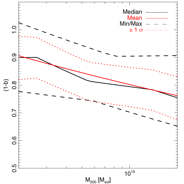
The bias $b$ can then be estimated from a comparison of observed and simulated relations, with the caveat that differences can also arise from imperfect modelling of cluster physics within the simulations. For the ensemble of simulations shown in Fig. 14, the right panel shows the ratio of the observed and simulated relations as a function of mass. Figure 15 shows the corresponding variation of $(1-b)$ as a function of mass $M$ from Eq. 27 for the observed slope $\alpha=1.79$. This is mass dependent due to the difference in slopes between the simulated and observed relations. At a pivot point of $M_{\mathrm{500}}=6\times 10^{14}\thinspace\mathrm{M}_{\odot}$, the median value of $A_{\mathrm{true}}/A_{\mathrm{obs}}$ is $0.74$, implying $(1-b)=0.81$. However, there is a large amount of scatter in the predictions from simulations. As a consequence, $(1-b)$ can vary from 0.74 to 0.97 at $M_{\mathrm{500}}=6\times 10^{14}\thinspace\mathrm{M}_{\odot}$. Note that the above results depend significantly on the baryon fraction $f_{\mathrm{b}}$. For example, assuming the WMAP-7 value $f_{\mathrm{b}}=0.167$, the median value of $(1-b)$ is $0.86$ at the pivot point of $M_{\mathrm{500}}=6\times 10^{14}\thinspace\mathrm{M}_{\odot}$.

A.4.3 Consistency with HE bias predictions and absolute calibration uncertainties

Taken at face value, the bias we derive above of $(1-b)\simeq 0.8$ implies that the HE mass used to calibrate the $Y_{500}$–$M_{\mathrm{500}}^{\mathrm{HE}}$ relation is offset from the true mass by around $20$ percent. Is this reasonable?

We can first compare HE X-ray and weak lensing (WL) masses. Although as mentioned above both measurements are expected to be biased, such comparisons are useful because the mass measurements involved are essentially independent. In addition measurements for moderately large sample sizes (tens of systems) are now starting to appear in the literature. However, at present there is little consensus, with some studies finding good agreement between HE and WL masses (e.g., Vikhlinin et al. 2009a; Zhang et al. 2010), some finding that HE masses are lower than WL masses, (e.g., Mahdavi et al. 2008), and some even finding that HE masses are higher than WL masses (Planck Collaboration Int. III 2013). The key point in such analyses is rigorous data quality on both the X-ray and optical sides. Most recent work points to relatively good agreement between X-ray and WL masses, with $M^{\mathrm{HE}}/M^{\mathrm{WL}}\simeq 0.9$ on average, and $M^{\mathrm{HE}}/M^{\mathrm{WL}}\simeq 1$ for relaxed systems (Mahdavi et al. 2013; von der Linden et al. 2012).

According to cosmological numerical simulations, the measurement bias induced by X-ray measurements relative to the ‘true’ values can be caused by two main effects. The first is the classic ‘hydrostatic mass bias’ due to non-thermal pressure support from turbulence/random motions, etc. However, the exact details are very model-dependent. The HE bias expected from simulations varies substantially, depending on the details of the numerical scheme, the input physics, and the approach used to calculate the HE masses (e.g., Rasia et al. 2012). In addition, the amount of bias is different depending on the dynamical state of the object, relaxed systems having less bias than unrelaxed systems. The majority of numerical simulations predict HE biases of 10 to 20 percent (Nagai et al. 2007; Piffaretti & Valdarnini 2008; Lau et al. 2009; Kay et al. 2012; Rasia et al. 2012).

Temperature inhomogeneities constitute the second contributor to X-ray measurement bias. In the presence of large amounts of cool gas, a single-temperature fit to a multi-temperature plasma will yield a result that is biased towards lower temperatures (e.g., Mazzotta et al. 2004). The presence of temperature inhomogeneities will depend on the dynamical state. While this effect can be investigated with simulations, estimates of its impact vary widely, owing to differences in numerical schemes and the different implementations of the input physics. For instance, simulations with heat conduction consistently predict smoother temperature distributions, thus X-ray spectroscopic biases are minimal in this case. On the other hand, ‘adiabatic’ simulations predict long-lasting high-density cool-core type phenomena, which will lead to significant biases in single-temperature fits. Estimates of biasing due to temperature inhomogeneities can range up to 10 or 15 percent (e.g., Rasia et al. 2012).

Finally, for HE mass estimates obtained from X-ray data, instrument calibration uncertainties also play a significant role in introducing uncertainties in mass estimates. For instance, the difference in calibration between XMM-Newton and Chandra can induce differences in $Y_{\mathrm{X}}$. This is typically $5$ percent, from a comparison of XMM-Newton based values published by Planck Collaboration XI (2011) to Chandra values for 28 ESZ clusters by Rozo et al. (2012b). This can lead to differences of up to 10 percent in the mass $M_{\mathrm{500}}^{Y_{\mathrm{X}}}$ derived from $Y_{\mathrm{X}}$, owing to the dependence of the mass on $Y_{\mathrm{X}}$.

Thus our adopted baseline value of $(1-b)\simeq 0.8$, ranging from $0.7$–$1$, appears to encompass our current ignorance of the exact bias.

A.5 Conclusions

In summary the baseline is

$$E^{-2/3}(z)\left[\frac{D_{\mathrm{A}}^{2}\thinspace Y_{500}}{\mathrm{10^{-4}\thinspace Mpc^{2}}}\right]=10^{-0.19\pm 0.02}\left[\frac{(1-b)M_{\mathrm{500}}}{6\times 10^{14}\mathrm{M}_{\odot}}\right]^{1.79\pm 0.08}\thinspace,$$ (28)

with an intrinsic scatter of $\sigma_{\log Y}=0.075$ and a mean bias $(1-b)=0.80_{-0.1}^{+0.2}$. The statistical uncertainty on the normalization is about $5\%$ and the error budget is dominated by the systematic uncertainties.