Compressive Shift Retrieval

Abstract

The classical shift retrieval problem considers two signals in vector form that are related by a shift. The problem is of great importance in many applications and is typically solved by maximizing the cross-correlation between the two signals. Inspired by compressive sensing, in this paper, we seek to estimate the shift directly from compressed signals. We show that under certain conditions, the shift can be recovered using fewer samples and less computation compared to the classical setup. Of particular interest is shift estimation from Fourier coefficients. We show that under rather mild conditions only one Fourier coefficient suffices to recover the true shift.

I Introduction

Shift retrieval is a fundamental problem in many signal processing applications. For example, to map the ocean floor, an active sonar can be used. The sonar transmits certain sound pulse patterns in the water, and the time it takes to receive the echoes of the pulses indicates the depth of the ocean floor. In target tracking using two acoustic sensors, the time shift when a sound wave of a vehicle reaches the microphones indicates the direction to the vehicle. In the case of a time shift, the shift retrieval problem is often referred to as time delay estimation (TDE) [3]. In computer vision, the spatial shift relating two images is often sought and referred to as image registration or alignment [4, 5, 6].

Traditionally, the shift retrieval problem is solved by maximizing the cross-correlation between the two signals [7]. In this paper, we revisit this classical problem, and show how the basic premise of compressive sensing (CS) [8, 9, 10, 11] can be used in the context of shift retrieval. This allows to recover the shift from compressed data leading to computational and storage savings.

Compressive sensing is a sampling scheme that makes it possible to sample at the information rate instead of the classical Nyquist rate predicted by the bandwidth of the signal [12]. The majority of the results in compressive sensing discuss conditions and methods for guaranteed reconstruction from an under-sampled version of the signal. Therefore, the information rate is typically referred to as the one that guarantees the recovery of the sparse signal.

However, for many applications such as the aforementioned examples in shift retrieval, obtaining the signal may not be needed. The goal is to recover some properties or statistics of the unknown signal. Taking the active sonar for example, one may wonder if it is really necessary to sample at a rate which is twice that of the bandwidth of the transmitted signal so that the received signal can be exactly reconstructed? Clearly the answer is no. Since the signal itself is not of interest to the application, we might consider an alternative sampling scheme to directly estimate the shift without first reconstructing the signal. These ideas have in fact been recently explored in the context of radar and ultrasound [13, 14, 15, 16] with continuous time signals and multiple shifts. Here we consider a related problem and ask: What is the minimal information rate to shift retrieval when two related discrete-time signals are under-sampled?

It turns out that under rather mild conditions, we only need fractions of the signals. In fact, we will show that only one Fourier coefficient from each of the signals suffices to recover the true shift. We refer to the method as compressive shift retrieval (CSR). It should be made clear that CSR does not assume that any of the involved signals are necessarily sparse.

As the main contribution of the paper, we will show that when the sensing matrix is taken to be a partial Fourier matrix, under suitable conditions, the true shift can be recovered from both noise-free and noisy measurements using CSR. Furthermore, CSR reduces both the computational load and the number of samples needed in the process. This is of particular interest since recent developments in sampling [17, 18, 19] have shown that Fourier coefficients can be efficiently obtained from space (or time) measurements by the use of an appropriate filter and by subsampling the output. Remarkably, our results also show that in some cases sampling as few as one Fourier coefficient is enough to perfectly recover the true shift.

I-A Prior Work

Compressive signal alignment problems have been addressed in only a few publications and, to the authors’ best knowledge, not in the same setup studied in this paper. In [20], the authors considered alignment of images under random projection. The work was based on the Johnson-Lindenstrauss property of random projection and proposed an objective function that can be solved efficiently using difference-of-two-convex programming algorithms. In this paper, we instead focus on proving theoretical guarantees of exact shift recovery when the signal is subsampled by a partial Fourier basis. The theory developed in [20] does not apply to this setup. The smashed filter [21] is another related technique. It is a general framework for maximum likelihood hypothesis testing and can be seen as a dimensionally reduced matched filter. It can therefore be applied to the shift retrieval problem. The underlying idea of both the smashed filter and CSR are the same in that both approaches try to avoid reconstructing the signal and extract the sought descriptor, namely, the shift, from compressive measurements. However, the analysis and assumptions are very different. For CSR, we develop requirements for guaranteed recovery of the true shift for a given measurement matrix. For the smashed filter, the analysis focuses on random orthoprojections and provides probabilities for correct recovery as a function of the number of projections. Also, in this paper, we are particularly interested in Fourier measurements, and many of the results are therefore tailored to this setting. The work presented here can therefore be seen as complementary to what was presented in [21] and its extension in [22].

I-B Notation and Assumptions

We use normal fonts to represent scalars and bold fonts for vectors and matrices. The notation $|\cdot|$ represents the absolute value for scalars, vectors and matrices, and it returns the cardinality of a set if the argument is a set. For both vectors and matrices, $\|\cdot\|_{0}$ is the $\ell_{0}$-norm function that returns the number of nonzero elements of its argument. Similarly, $\|\cdot\|_{p}$ represents the $\ell_{p}$-norm. For a vector ${\boldsymbol{x}}$, the $\ell_{p}$-norm is defined as $\|{{\boldsymbol{x}}}\|_{p}\triangleq(\sum_{i}|x_{i}|^{p})^{1/p}$, where $x_{i}$ is the $i$th element of ${\boldsymbol{x}}$. For a matrix ${\boldsymbol{X}}$, $\|\cdot\|_{p}$ is defined as ${{\boldsymbol{X}}}\triangleq(\sum_{i,j}|{X}_{i,j}|^{p})^{1/p}$, where ${X}_{i,j}$ is the $(i,j)$-th element of ${\boldsymbol{X}}$. Furthermore, ${\boldsymbol{X}}^{*}$ denotes the complex conjugate transpose of ${\boldsymbol{X}}$. Let ${\boldsymbol{I}}_{n\times n}$ denote an $n\times n$ identity matrix, ${\boldsymbol{0}}_{m\times n}$ an $m\times n$ matrix of zeros, and $\mathbb{Z}$ be the set of integers. $\Re\{\cdot\}$ returns the real part of its argument. We say that two $n$-dimensional vectors ${\boldsymbol{y}}$ and ${\boldsymbol{x}}$ are related by an $l$ cyclic-shift if ${\boldsymbol{y}}={\boldsymbol{D}}^{l}{\boldsymbol{x}}$, where ${\boldsymbol{D}}^{l}$ is defined as

$${\boldsymbol{D}}^{l}=\begin{bmatrix}{\boldsymbol{0}}_{l\times(n-l)}&{\boldsymbol{I}}_{l\times l}\\ {\boldsymbol{I}}_{(n-l)\times(n-l)}&{\boldsymbol{0}}_{(n-l)\times l}\end{bmatrix}.$$ (1)

Throughout the paper, we will assume that the shift is unique up to a multiple of $n$. Also note that we are considering cyclic shifts.

I-C Organization

In Sections II and III, we study the CSR problem under the assumption that the measurements are noise free. Next, we extend the results to noisy measurements in Section IV. As we are particularly interested in Fourier measurements, we will tailor the results to this particular choice of sensing matrix. Section V concludes the paper. All proofs are provided in the Appendice for clarity.

II Noise-Free Compressive Shift Retrieval

The shift retrieval problem is a multi-hypothesis testing problem: Define the $s$th hypothesis $\mathcal{H}_{s}$, $s=0,\dots,n-1$, as

$$\mathcal{H}_{s}:\>{\boldsymbol{x}}\text{ is related to } {\boldsymbol{y}}\text{ via a }s\text{-cyclic-shift},$$

and accept $\mathcal{H}_{s}$ if ${\boldsymbol{y}}={\boldsymbol{D}}^{s}{\boldsymbol{x}}$ and otherwise reject. Since the true shift is assumed unique, only one hypothesis will be accepted and the corresponding shift is necessarily the true solution. The connection to the cross-correlation is now trivial:

$$\|{\boldsymbol{y}}-{\boldsymbol{D}}^{s}{\boldsymbol{x}}\|_{2}^{2}= \|{\boldsymbol{y}}\|^{2}_{2}+\|{\boldsymbol{D}}^{s}{\boldsymbol{x}}\|_{2}^{2}-{\boldsymbol{y}}^{*}{\boldsymbol{D}}^{s}{\boldsymbol{x}}-{\boldsymbol{D}}^{s}{\boldsymbol{x}}^{*}{\boldsymbol{y}}$$

$$= \|{\boldsymbol{y}}\|^{2}_{2}+\|{\boldsymbol{x}}\|_{2}^{2}-2\Re\{\langle{\boldsymbol{y}},{\boldsymbol{D}}^{s}{\boldsymbol{x}}\rangle\}$$ (2)

where we use the fact that $\|{\boldsymbol{D}}^{s}{\boldsymbol{x}}\|_{2}^{2}=\|{\boldsymbol{x}}\|_{2}^{2}$. Since $\|{\boldsymbol{y}}-{\boldsymbol{D}}^{s}{\boldsymbol{x}}\|_{2}^{2}\geq 0$, equating ${\boldsymbol{y}}={\boldsymbol{D}}^{s}{\boldsymbol{x}}$ is equivalent to minimizing $\|{\boldsymbol{y}}-{\boldsymbol{D}}^{s}{\boldsymbol{x}}\|_{2}^{2}$ or maximizing the real part of the cross-correlation with respect to $s$:

$$\max\Re\{\langle{\boldsymbol{y}},{\boldsymbol{D}}^{s}{\boldsymbol{x}}\rangle\}.$$ (3)

Now, assume that the compressed measurement signals ${\boldsymbol{z}}={\boldsymbol{A}}{\boldsymbol{y}}\in\mathbb{C}^{m}$ and ${\boldsymbol{v}}={\boldsymbol{A}}{\boldsymbol{x}}\in\mathbb{C}^{m}$ are given and related to the ground-truth signals ${\boldsymbol{x}}\in\mathbb{C}^{n}$ and its shifted version ${\boldsymbol{y}}={\boldsymbol{D}}^{l}{\boldsymbol{x}}\in\mathbb{C}^{n}$ via the sensing matrix ${\boldsymbol{A}}\in\mathbb{C}^{m\times n}$, $m<n$. The goal of CSR is to recover the shift $l$ relating ${\boldsymbol{x}}$ and ${\boldsymbol{y}}$ from the compressed measurements ${\boldsymbol{z}}$ and ${\boldsymbol{v}}$.

Since only the compressed measurements ${\boldsymbol{z}}$ and ${\boldsymbol{v}}$ are assumed available, we can not evaluate ${\boldsymbol{y}}={\boldsymbol{D}}^{s}{\boldsymbol{x}}$ or maximize $\Re\{\langle{\boldsymbol{y}},{\boldsymbol{D}}^{s}{\boldsymbol{x}}\rangle\}$ for each hypothesis ${\boldsymbol{D}}^{s}$. However, if ${\boldsymbol{A}}^{*}{\boldsymbol{A}}$ and ${\boldsymbol{D}}^{s}$ commute for all $s=0,\dots,n-1$, then

$${\boldsymbol{y}}={\boldsymbol{D}}^{s}{\boldsymbol{x}}\quad\Rightarrow \quad{\boldsymbol{A}}^{*}{\boldsymbol{A}}{\boldsymbol{y}}={\boldsymbol{A}}^{*}{\boldsymbol{A}}{\boldsymbol{D}}^{s}{\boldsymbol{x}}={\boldsymbol{D}}^{s}{\boldsymbol{A}}^{*}{\boldsymbol{A}}{\boldsymbol{x}}$$

$$\Leftrightarrow \quad{\boldsymbol{A}}^{*}{\boldsymbol{z}}={\boldsymbol{D}}^{s}{\boldsymbol{A}}^{*}{\boldsymbol{v}}.$$ (4)

Hence, we could consider the test:

$$\text{Accept }\mathcal{H}_{s}\text{ if }{\boldsymbol{A}}^{*}{\boldsymbol{z}}={\boldsymbol{D}}^{s}{\boldsymbol{A}}^{*}{\boldsymbol{v}}\text{ and otherwise reject}.$$ (5)

It is clear that if $s$ is such that ${\boldsymbol{y}}={\boldsymbol{D}}^{s}{\boldsymbol{x}}$, then ${\boldsymbol{A}}^{*}{\boldsymbol{z}}={\boldsymbol{D}}^{s}{\boldsymbol{A}}^{*}{\boldsymbol{v}}$ will also hold. However, the other way around might not be true. Therefore, we might erroneously accept a wrong hypotheses using (5). The next theorem lists the conditions by which the testing (5) is guaranteed to accept the correct hypothesis. Notice that testing the condition ${\boldsymbol{A}}^{*}{\boldsymbol{z}}={\boldsymbol{D}}^{s}{\boldsymbol{A}}^{*}{\boldsymbol{v}}$ is equivalent to minimizing $\|{\boldsymbol{A}}^{*}{\boldsymbol{z}}-{\boldsymbol{D}}^{s}{\boldsymbol{A}}^{*}{\boldsymbol{v}}\|_{2}^{2}$ with respect to $s$.

Theorem 1 (Shift Recovery from Low-Rate Data).

Let ${\boldsymbol{X}}$ be an $n\times n$ matrix with the $i$th column equal to ${\boldsymbol{D}}^{i}{\boldsymbol{x}}$, $i=1,\dots,n,$ and define $\bar{\boldsymbol{D}}^{s}={\boldsymbol{A}}{\boldsymbol{D}}^{s}{\boldsymbol{A}}^{*}$. If the sensing matrix ${\boldsymbol{A}}$ satisfies the following conditions:

• ${\boldsymbol{A}}^{*}{\boldsymbol{A}}{\boldsymbol{D}}^{s}={\boldsymbol{D}}^{s}{\boldsymbol{A}}^{*}{\boldsymbol{A}}$,

• $\exists\alpha\in{\mathbb{R}},\alpha{\boldsymbol{A}}{\boldsymbol{A}}^{*}={\boldsymbol{I}}$ and

• all columns of ${\boldsymbol{A}}{\boldsymbol{X}}$ are different,

then

$$\max_{s}\Re\{\langle{\boldsymbol{z}},\bar{\boldsymbol{D}}^{s}{\boldsymbol{v}}\rangle\}$$ (6)

or equivalently the test (5) recovers the true shift.

The conditions of Theorem 1 may seem restrictive. However, as we will show in Lemma 3, if ${\boldsymbol{A}}$ is chosen as a partial Fourier matrix, then the first two conditions of Theorem 1 are trivially satisfied. The last condition is the only one that needs to be checked and will lead to a condition on the sampled Fourier coefficients.

The conditions of Theorem 1 can be checked prior to estimating the shift. However, knowing the estimate of the shift, it is easy to see from the proof (see the proof of Lemma 8) that it is enough to check if the column of ${\boldsymbol{A}}{\boldsymbol{X}}$ associated with the estimate of the shift is different than all the other columns of ${\boldsymbol{A}}{\boldsymbol{X}}$. Hence, we do not need to check if all columns of ${\boldsymbol{A}}{\boldsymbol{X}}$ are different. This conclusion is formulated in the following corollary, which is less conservative than Theorem 1.

Corollary 2 (Test for True Shift).

Let ${\boldsymbol{X}}$ be an $n\times n$ matrix with the $i$th column equal to ${\boldsymbol{D}}^{i}{\boldsymbol{x}}$, $i=1,\dots,n,$ and define $\bar{\boldsymbol{D}}^{s}={\boldsymbol{A}}{\boldsymbol{D}}^{s}{\boldsymbol{A}}^{*}$. If the sensing matrix ${\boldsymbol{A}}$ satisfies the following conditions:

• ${\boldsymbol{A}}^{*}{\boldsymbol{A}}{\boldsymbol{D}}^{s}={\boldsymbol{D}}^{s}{\boldsymbol{A}}^{*}{\boldsymbol{A}}$, and

• $\exists\alpha\in{\mathbb{R}},\alpha{\boldsymbol{A}}{\boldsymbol{A}}^{*}={\boldsymbol{I}}$,

then

$$s^{*}=\mathop{\rm arg\,max}_{s}\Re\{\langle{\boldsymbol{z}},\bar{\boldsymbol{D}}^{s}{\boldsymbol{v}}\rangle\}$$ (7)

is the true shift if the $s^{*}$th column of ${\boldsymbol{A}}{\boldsymbol{X}}$ is different than all the other columns of ${\boldsymbol{A}}{\boldsymbol{X}}$.

III Compressive Shift Retrieval using Fourier Coefficients

Of particular interest is the case where ${\boldsymbol{A}}$ is made up of a partial Fourier basis. That is, ${\boldsymbol{A}}$ takes the form

$${\boldsymbol{A}}=\frac{1}{\sqrt{n}}\begin{bmatrix}1&e^{-\frac{2j\pi k_{1}}{n}}&e^{-\frac{4j\pi k_{1}}{n}}&\cdots&e^{-\frac{2(n-1)j\pi k_{1}}{n}}\\ 1&e^{-\frac{2j\pi k_{2}}{n}}&\ddots&&e^{-\frac{2(n-1)j\pi k_{2}}{n}}\\ \vdots&\vdots&&&\\ 1&e^{-\frac{2j\pi k_{m}}{n}}&e^{-\frac{4j\pi k_{m}}{n}}&\cdots&e^{-\frac{2(n-1)j\pi k_{m}}{n}}\end{bmatrix}$$

where $k_{1},\dots,k_{m}\in\{0,1,2,\dots n-1\},m\leq n$. For this specific choice,

$${\boldsymbol{A}}{\boldsymbol{X}}=\frac{1}{\sqrt{n}}\begin{bmatrix}X_{k_{1}}&X_{k_{1}}e^{\frac{2k_{1}\pi j}{n}}&\cdots&X_{k_{1}}e^{\frac{2(n-1)k_{1}\pi j}{n}}\\ X_{k_{2}}&\ddots&&X_{k_{2}}e^{\frac{2(n-1)k_{2}\pi j}{n}}\\ \vdots&&&\\ X_{k_{m}}&X_{k_{m}}e^{\frac{2k_{m}\pi j}{n}}&\cdots&X_{k_{m}}e^{\frac{2(n-1)k_{m}\pi j}{n}}\end{bmatrix}$$

where $X_{r}$ denotes the $r$th Fourier coefficient of the Fourier transform of ${\boldsymbol{x}}$.

For a sensing matrix made up by a partial Fourier basis, we have the following useful result:

Lemma 3.

Let ${\boldsymbol{A}}$ be a partial Fourier matrix. Then ${\boldsymbol{D}}^{s}{\boldsymbol{A}}^{*}{\boldsymbol{A}}={\boldsymbol{A}}^{*}{\boldsymbol{A}}{\boldsymbol{D}}^{s}$ for all $s=1,\dots,n$.

Using this result in Theorem 1 gives the following corollary:

Corollary 4 (Shift Recovery from Low Rate Fourier Data).

With ${\boldsymbol{A}}$ denoting a partial Fourier matrix and $z_{i}$ and $v_{i}$ the $i$th element of ${\boldsymbol{z}}$ and ${\boldsymbol{v}}$,

$$\max_{s}\Re\left\{\sum_{i=1}^{m}z_{i}v_{i}e^{\frac{-2\pi jk_{i}s}{n}}\right\}$$ (8)

recovers the true shift if there exists $p\in\{1,\dots,m\}$ such that $X_{k_{p}}\neq 0$ and $\{1,\dots,n-1\}\frac{k_{p}}{n}$ contains no integers. In particular, measuring only the first Fourier coefficients ($k_{1}=1$) of ${\boldsymbol{x}}$ and ${\boldsymbol{y}}$ would, as long as the coefficients are nonzero, suffice to recover the true shift.

Remarkably, in the extreme case when $m=1$, the corollary states that all we need is two scalar measurements, $z$ and $v$, to perfectly recover the true shift. The scalar measurements can be any nonzero Fourier coefficient of ${\boldsymbol{x}}$ and ${\boldsymbol{y}}$ as long as $\{1,\dots,n-1\}\frac{k_{1}}{n}$ contains no integers. As noted in the corollary, the first Fourier coefficients ($k_{1}=1$) of ${\boldsymbol{x}}$ and ${\boldsymbol{y}}$ would suffice. Also note that only $2mn$ multiplications are required to evaluate the test. This should be compared with $n^{2}$ multiplications to evaluate the cross-correlation for the full uncompressed signals ${\boldsymbol{x}}$ and ${\boldsymbol{y}}$. Corollary 4 is easy to check but more conservative than both Theorem 1 and Corollary 2.

To validate the results, we carried out the following example. In each trial we let the sample dimension $m$ and the shift $l$ be random integers between 1 and 9 and generate ${\boldsymbol{x}}$ by sampling from a $n$-dimensional uniform distribution. We let $n=10$ and make sure that ${\boldsymbol{A}}$ in each trial is a partial Fourier basis satisfying the assumptions of Corollary 4. We carry out 10000 trials. The true shift is successfully recovered in each trial by the simplified test (8), namely, with 100% success rate. This is quite remarkable since when $m=1$, we recover the true shift using only two scalar measurement ${\boldsymbol{z}}$ and ${\boldsymbol{v}}$ and $1/5$ of the multiplications that maximizing the real part of inner product between the original signals (3) would need.

IV Noisy Compressive Shift Retrieval

Now we consider the noisy version of compressive shift retrieval, where the measurements ${\boldsymbol{z}}$ and ${\boldsymbol{v}}$ are perturbed by noise:

$$\tilde{\boldsymbol{z}}={\boldsymbol{z}}+{\boldsymbol{e}}_{z},\quad\tilde{\boldsymbol{v}}={\boldsymbol{v}}+{\boldsymbol{e}}_{v}.$$ (9)

Similar to the noise-free case, here we can also guarantee the recovery of the true shift. Our main result is given in the following theorem:

Theorem 5 (Noisy Shift Recovery from Low-Rate Data).

Let $\tilde{\boldsymbol{x}}$ be such that $\tilde{\boldsymbol{v}}={\boldsymbol{A}}\tilde{\boldsymbol{x}}$, the $i$th column of $\tilde{\boldsymbol{X}}$ be shifted versions of $\tilde{\boldsymbol{x}}$, and assume that ${\boldsymbol{A}}$ is a partial Fourier matrix and that the noisy measurements are used in (8) to estimate the shift. If the $\ell_{2}$-norm difference between any two columns of ${\boldsymbol{A}}\tilde{\boldsymbol{X}}$ is greater than

$$\Delta_{{\boldsymbol{z}}{\boldsymbol{v}}}\triangleq\|{\boldsymbol{e}}_{z}\|_{2}+\|{\boldsymbol{e}}_{v}\|_{2}+\sqrt{\|\tilde{\boldsymbol{v}}\|_{2}^{2}+\|\tilde{\boldsymbol{z}}\|_{2}^{2}-2\max_{s}\Re\{\langle\tilde{\boldsymbol{z}},\bar{\boldsymbol{D}}^{s}\tilde{\boldsymbol{v}}\rangle\}},$$

then the estimate of the shift is not affected by the noise.

Note that the theorem only states that the noise does not affect the estimate of the shift. It does not state that the shift will be the true shift.

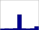
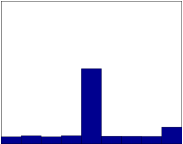
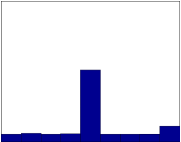
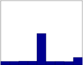
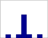
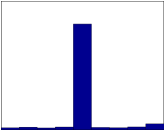
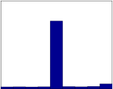
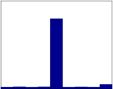
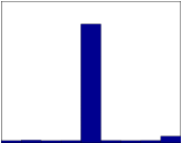
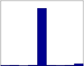
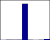
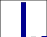
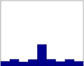
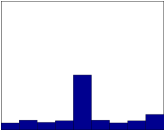
We illustrate the results by running a Monte Carlo simulation consisting of 10000 trials for each sample dimension $m=1,\dots,10,$ and for two different SNR levels. In Figure 1, 10 histograms are shown (corresponding to $m=1,\dots,10$) for the

$$\text{SNR}=\frac{\|{\boldsymbol{z}}\|_{2}^{2}}{\|\tilde{\boldsymbol{z}}-{\boldsymbol{z}}\|_{2}^{2}}$$ (10)

being 2 (low SNR) and in Figure 2, $SNR=10$ (high SNR). The errors ${\boldsymbol{e}}_{z}$ and ${\boldsymbol{e}}_{x}$ were both generated by sampling from

$$\mathcal{N}(0,\sigma^{2})+j\mathcal{N}(0,\sigma^{2}).$$ (11)

We further use $n=10$, $l=5$ and sample ${\boldsymbol{x}}$ from a uniform (0,1)-distribution. The conclusion from the simulation is that the smaller the $m$, the more the estimate of the shift is sensitive to noise. Notice that when $m=10$ the test (8) reduces to the classical test of maximizing the cross-correlation.

We can now use Theorem 5 to check if the noise affected the estimate of the shift or not in each of the trials. For $m=2$ and the high SNR, 40% of the trials satisfied the conditions of Theorem 5 and the noise therefore did not affect the shift estimates in those cases. Of the trails that satisfied the conditions, all predicted the true shift and none a false shift. Note however that Theorem 5 only states that if the conditions are satisfied, then the estimated shift is the same as if we would have used the noise free compressed measurements in the test (8). It does not state that the estimate will be the true shift.

Figure 1: Histogram plots for the estimated shift and low SNR. From left to right, top to bottom, $m=1,\dots,10$. The true shift was set to 5 in all trials.

Figure 2: Histogram plots for the estimated shift and high SNR. From left to right, top to bottom, $m=1,\dots,10$. The true shift was set to 5 in all trials.

Theorem 5 gives conditions for when the noise does not affect the estimate of the shift. This is a good property but even better would be if the recovery of the true shift could be guaranteed. This is given by the following corollary.

Corollary 6 (Recovery of the True Shift from Noisy Low-Rate Data).

If the $\ell_{2}$-norm difference between any two columns of ${\boldsymbol{A}}\tilde{\boldsymbol{X}}$ is greater than $2\|{\boldsymbol{e}}_{v}\|_{2}$ and the conditions of Theorem 5 are fulfilled, then (8) recovers the true shift.

If the estimate of the shift has been computed, a less conservative test can be used to check if the computed estimate has been affected by noise and if it is the true one. We summarize our conclusion in the following corollary.

Corollary 7 (Test for True Shift in the Presence of Noise).

Assume that (8) gives $s^{*}$ as an estimate of the shift. If the $\ell_{2}$ difference between any column and the $s^{*}$-column of ${\boldsymbol{A}}\tilde{\boldsymbol{X}}$ is greater than $2\|{\boldsymbol{e}}_{v}\|_{2}$ and $\Delta_{{\boldsymbol{z}}{\boldsymbol{v}}}$, then $s^{*}$ is the true shift.

V Conclusion

To recover the cyclic shift relating two 1D signals, the cross-correlation is usually evaluated for all possible shifts. Recent advances in hardware, signal acquisition and signal processing have made it possible to sample or compute Fourier coefficients of a signal efficiently. It is therefore of particular interest to see under what conditions the true shift can be recovered from the Fourier coefficients. We have proposed a criterion that is computationally more efficient than using the time samples, and we have shown that the true shift can be recovered using as few as one Fourier coefficient. We have also derived bounds for perfect recovery for both noise free and noisy measurements.

Appendix A Proofs: Noise-Free Compressive Shift Retrieval

Before proving the Theorem 1, we state two lemmas.

Lemma 8 (Recovery of Shift using Projections).

Let ${\boldsymbol{X}}$ be the $n\times n$-matrix made up of cyclically shifted versions of ${\boldsymbol{x}}$ as columns. If the columns of ${\boldsymbol{A}}{\boldsymbol{X}}$ are distinct, then the true shift can be recovered by

$$\min_{{\boldsymbol{q}}\in\{0,1\}^{n}}\|{\boldsymbol{A}}{\boldsymbol{y}}-{\boldsymbol{A}}{\boldsymbol{X}}{\boldsymbol{q}}\|_{2}^{2}\quad\text{s.t.}\quad\|{\boldsymbol{q}}\|_{0}=1.$$ (12)

Proof of Lemma 8.

Since the shift relating ${\boldsymbol{x}}$ and ${\boldsymbol{y}}$ is assumed unique, it is clear that the true shift is recovered by

$$\min_{{\boldsymbol{q}}\in\{0,1\}^{n}}\|{\boldsymbol{y}}-{\boldsymbol{X}}{\boldsymbol{q}}\|_{2}^{2}\quad\text{s.t.}\quad\|{\boldsymbol{q}}\|_{0}=1.$$ (13)

Assume that the solution of (12) is not equivalent to that of (13). Namely, assume that (13) gives ${\boldsymbol{q}}$, (12) gives $\tilde{\boldsymbol{q}}$ and ${\boldsymbol{q}}\neq\tilde{\boldsymbol{q}}$. Since ${\boldsymbol{q}}$ will give a zero objective value in (12), so must $\tilde{\boldsymbol{q}}$. We therefore have that ${\boldsymbol{A}}{\boldsymbol{y}}={\boldsymbol{A}}{\boldsymbol{X}}\tilde{\boldsymbol{q}}={\boldsymbol{A}}{\boldsymbol{X}}{\boldsymbol{q}}$ and hence

$${\boldsymbol{A}}{\boldsymbol{X}}\tilde{\boldsymbol{q}}-{\boldsymbol{A}}{\boldsymbol{X}}{\boldsymbol{q}}={\boldsymbol{A}}{\boldsymbol{X}}(\tilde{\boldsymbol{q}}-{\boldsymbol{q}})=0.$$ (14)

Since ${\boldsymbol{q}},\,\tilde{\boldsymbol{q}}\in\{0,1\}^{n}$, $\|\tilde{\boldsymbol{q}}\|_{0}=\|{\boldsymbol{q}}\|_{0}=1$, and ${\boldsymbol{q}}\neq\tilde{\boldsymbol{q}}$, ${\boldsymbol{A}}{\boldsymbol{X}}(\tilde{\boldsymbol{q}}-{\boldsymbol{q}})=0$ implies that two columns of ${\boldsymbol{A}}{\boldsymbol{X}}$ are identical. This is a contradiction and we therefore conclude that both (12) and (13) recover the true shift. ∎

Lemma 9 (From (12) to (6)).

Under conditions 1) and 2) of Theorem 1, the shifts recovered by (12) and (6) are the same.

Proof of Lemma 9.

Consider the objective of (12):

$$\|{\boldsymbol{A}}{\boldsymbol{y}}-{\boldsymbol{A}}{\boldsymbol{X}}{\boldsymbol{q}}\|_{2}^{2}= ({\boldsymbol{A}}{\boldsymbol{y}})^{*}{\boldsymbol{A}}{\boldsymbol{y}}+({\boldsymbol{A}}{\boldsymbol{X}}{\boldsymbol{q}})^{*}{\boldsymbol{A}}{\boldsymbol{X}}{\boldsymbol{q}}$$

$$- ({\boldsymbol{A}}{\boldsymbol{y}})^{*}{\boldsymbol{A}}{\boldsymbol{X}}{\boldsymbol{q}}-({\boldsymbol{A}}{\boldsymbol{X}}{\boldsymbol{q}})^{*}{\boldsymbol{A}}{\boldsymbol{y}}.$$ (15)

Writing ${\boldsymbol{X}}{\boldsymbol{q}}={\boldsymbol{D}}^{s}{\boldsymbol{x}}$, problem (12) is equal to

$$\max_{s}2\Re\{({\boldsymbol{A}}{\boldsymbol{y}})^{*}{\boldsymbol{A}}{\boldsymbol{D}}^{s}{\boldsymbol{x}}\}-({\boldsymbol{A}}{\boldsymbol{D}}^{s}{\boldsymbol{x}})^{*}{\boldsymbol{A}}{\boldsymbol{D}}^{s}{\boldsymbol{x}}.$$ (16)

Now, if ${\boldsymbol{A}}^{*}{\boldsymbol{A}}{\boldsymbol{D}}^{s}={\boldsymbol{D}}^{s}{\boldsymbol{A}}^{*}{\boldsymbol{A}}$ and using that $({\boldsymbol{D}}^{s})^{*}{\boldsymbol{D}}^{s}={\boldsymbol{I}}$ for a shift matrix, then

$$({\boldsymbol{A}}{\boldsymbol{D}}^{s}{\boldsymbol{x}})^{*}{\boldsymbol{A}}{\boldsymbol{D}}^{s}{\boldsymbol{x}}={\boldsymbol{x}}^{*}({\boldsymbol{D}}^{s})^{*}{\boldsymbol{A}}^{*}{\boldsymbol{A}}{\boldsymbol{D}}^{s}{\boldsymbol{x}}=\|{\boldsymbol{A}}{\boldsymbol{x}}\|_{2}^{2},$$ (17)

which is independent of $s$. Therefore, the shift recovered by (16) is the same as that of

$$\max_{s}\Re\{({\boldsymbol{A}}{\boldsymbol{y}})^{*}{\boldsymbol{A}}{\boldsymbol{D}}^{s}{\boldsymbol{x}}\}.$$ (18)

Lastly, if we again use that ${\boldsymbol{A}}^{*}{\boldsymbol{A}}{\boldsymbol{D}}^{s}={\boldsymbol{D}}^{s}{\boldsymbol{A}}^{*}{\boldsymbol{A}}$ and $\alpha{\boldsymbol{A}}{\boldsymbol{A}}^{*}={\boldsymbol{I}}$, then (6) follows from

$$\Re\{({\boldsymbol{A}}{\boldsymbol{y}})^{*}{\boldsymbol{A}}{\boldsymbol{D}}^{s}{\boldsymbol{x}}\} =\Re\{{\boldsymbol{y}}^{*}{\boldsymbol{A}}^{*}{\boldsymbol{A}}{\boldsymbol{D}}^{s}{\boldsymbol{x}}\}$$ (19)

$$=\alpha\Re\{{\boldsymbol{y}}^{*}{\boldsymbol{A}}^{*}{\boldsymbol{A}}{\boldsymbol{A}}^{*}{\boldsymbol{A}}{\boldsymbol{D}}^{s}{\boldsymbol{x}}\}$$ (20)

$$=\alpha\Re\{{\boldsymbol{y}}^{*}{\boldsymbol{A}}^{*}{\boldsymbol{A}}{\boldsymbol{D}}^{s}{\boldsymbol{A}}^{*}{\boldsymbol{A}}{\boldsymbol{x}}\}$$ (21)

$$=\alpha\Re\{\langle{\boldsymbol{z}},\bar{\boldsymbol{D}}^{s}{\boldsymbol{v}}\rangle\}$$ (22)

where ${\boldsymbol{z}}={\boldsymbol{A}}{\boldsymbol{y}}$ and ${\boldsymbol{v}}={\boldsymbol{A}}{\boldsymbol{x}}$. ∎

We are now ready to prove Theorem 1.

Proof of Theorem 1.

The assumptions of Theorem 1 imply that requirements of both Lemmas 8 and 9 are satisfied. The theorem therefore follows trivially. ∎

We next prove Corollary 2.

Proof of Corollary 2.

In the proof of Lemma 8, ${\boldsymbol{A}}{\boldsymbol{X}}(\tilde{\boldsymbol{q}}-{\boldsymbol{q}})=0$ leads to $\tilde{\boldsymbol{q}}-{\boldsymbol{q}}=0$ if the columns of ${\boldsymbol{A}}{\boldsymbol{X}}$ were all distinct. Now, if

$$s^{*}=\mathop{\rm arg\,max}_{s}\Re\{\langle{\boldsymbol{z}},\bar{\boldsymbol{D}}^{s}{\boldsymbol{v}}\rangle\},$$ (23)

that corresponds to the $s^{*}$th element of $\tilde{\boldsymbol{q}}$ being one and all other elements zero. Hence, Lemma 8 can be made less conservative if $s^{*}$ is known by requiring that only the $s^{*}$th column of ${\boldsymbol{A}}{\boldsymbol{X}}$ is different than all other columns. ∎

Proof of Lemma 3.

Let ${\boldsymbol{M}}={\boldsymbol{A}}{\boldsymbol{D}}^{s}$ and ${\boldsymbol{Q}}={\boldsymbol{A}}({\boldsymbol{D}}^{s})^{*}$. By the definition of ${\boldsymbol{D}}^{s}$, ${\boldsymbol{M}}$ is a column permutation of ${\boldsymbol{A}}$ where the columns are shifted $s$ times to the right. Thus, the $r$th column of ${\boldsymbol{M}}$ is equal to the $t$th column of ${\boldsymbol{A}}$ where $t=(r-s)\text{ mod }n$. It is also easy to see that $({\boldsymbol{D}}^{s})^{*}$ permutes the columns of ${\boldsymbol{A}}$ by $s$ to the left so that the $r$th column of ${\boldsymbol{Q}}$ is equal to the $q$th column of ${\boldsymbol{A}}$ where $q=(r+s)\text{ mod }n$. Now, the $pr$th element of ${\boldsymbol{A}}^{*}{\boldsymbol{M}}={\boldsymbol{A}}^{*}{\boldsymbol{A}}{\boldsymbol{D}}^{s}$ is given by

$$({\boldsymbol{A}}_{:,p})^{*}{\boldsymbol{M}}_{:,r}=({\boldsymbol{A}}_{:,p})^{*}{\boldsymbol{A}}_{:,r-s}=\frac{1}{n}\sum_{i=1}^{m}e^{2j\pi k_{i}(p-r+s)},$$ (24)

where ${\boldsymbol{A}}_{:,p}$ is used to denote the $p$th column of ${\boldsymbol{A}}$ and ${\boldsymbol{M}}_{:,r}$ the $r$th column or ${\boldsymbol{M}}$. On the other hand, the $(p,r)$-th element of ${\boldsymbol{Q}}^{*}{\boldsymbol{A}}={\boldsymbol{D}}^{s}{\boldsymbol{A}}^{*}{\boldsymbol{A}}$ is given by

$$({\boldsymbol{Q}}_{:,p})^{*}{\boldsymbol{A}}_{:,r}=({\boldsymbol{A}}_{:,p+s})^{*}{\boldsymbol{A}}_{:,r}=\frac{1}{n}\sum_{i=1}^{m}e^{2j\pi k_{i}(p+s-r)}.$$ (25)

Clearly, the two are equivalent. ∎

We are now ready to prove Corollary 4.

Proof of Corollary 4.

Lemma 3 gives that Condition 1) of Theorem 1 is satisfied. Since a full Fourier matrix is orthonormal, a matrix made up of a selection of rows of a Fourier matrix satisfies Condition 2). The last condition of Theorem 1 requires columns of ${\boldsymbol{A}}{\boldsymbol{X}}$ to be distinct. A sufficient condition is that there exists a row with all distinct elements. As shown previously, the $(p,r)$-th element of ${\boldsymbol{A}}{\boldsymbol{X}}$ is $X_{k_{p}}e^{\frac{2j\pi k_{p}(r-1)}{n}}.$ If $X_{k_{p}}$ is assumed nonzero, a sufficient condition for ${\boldsymbol{A}}{\boldsymbol{X}}$ to have distinct columns is that $e^{\frac{2j\pi k_{p}r_{1}}{n}}\neq e^{\frac{2j\pi k_{p}r_{2}}{n}},\,r_{1},r_{2}\in\{0,\dots,n-1\},r_{1}\neq r_{2}$. This condition can be simplified to $\frac{k_{p}r_{1}}{n}\neq\frac{k_{p}r_{2}}{n}+\gamma,\,\gamma\in{\mathbb{Z}}$. By realizing that $r_{1}-r_{2}$ takes values in $\{-n+1,\dots,-1,1,\dots,n-1\}$ we get that the condition is equivalent to requiring that there is no integers in $\{-n+1,\dots,-1,1,\dots,n-1\}\frac{k_{p}}{n}$. Due to symmetry, a sufficient condition for distinct columns is that there exists a $p\in\{1,\dots,m\}$ such that $X_{k_{p}}\neq 0$ and $\{1,\dots,n-1\}\frac{k_{p}}{n}$ contains no integers. Lastly, if we write out ${\boldsymbol{A}}{\boldsymbol{D}}^{s}{\boldsymbol{A}}^{*}$ we get that the $pr$th element is equal to $\delta_{p,r}e^{-\frac{2j\pi k_{p}s}{n}}/n$ and hence the simplified test proposed in (8). ∎

Appendix B Proofs: Noisy Compressive Shift Retrieval

Proof of Theorem 5.

From Lemma 9 we can see that seeking $s$ that maximizes $\Re\{\langle\tilde{\boldsymbol{z}},\bar{\boldsymbol{D}}^{s}\tilde{\boldsymbol{v}}\rangle\}$ is equivalent to seeking ${\boldsymbol{q}}$ that solves

$$\min_{{\boldsymbol{q}}\in\{0,1\}^{n}}\|\tilde{\boldsymbol{z}}-{\boldsymbol{A}}\tilde{\boldsymbol{X}}{\boldsymbol{q}}\|_{2}^{2}\quad\text{s.t.}\quad\|{\boldsymbol{q}}\|_{0}=1,$$ (26)

where the first column of ${\boldsymbol{A}}\tilde{\boldsymbol{X}}$ is equal to $\tilde{\boldsymbol{v}}$ (which defines the first column of $\tilde{\boldsymbol{X}}$) and the $i$th column of $\tilde{\boldsymbol{X}}$ a circular shift of the first column $i-1$ steps. Assume that $\hat{\boldsymbol{q}}$ solves (26). Since our measurements are noisy, we can not expect a zero loss. The loss can be shown given by

$$\|\tilde{\boldsymbol{z}}-{\boldsymbol{A}}\tilde{\boldsymbol{X}}\hat{\boldsymbol{q}}\|_{2}^{2}=\|\tilde{\boldsymbol{v}}\|_{2}^{2}+\|\tilde{\boldsymbol{z}}\|_{2}^{2}-\max_{s}2\Re\{\tilde{\boldsymbol{z}}^{*}\bar{\boldsymbol{D}}^{s}\tilde{\boldsymbol{v}}\}.$$ (27)

Now, consider $\|\tilde{\boldsymbol{z}}-{\boldsymbol{A}}\tilde{\boldsymbol{X}}\hat{\boldsymbol{q}}\|_{2}$. Assume that ${\boldsymbol{q}}_{0}$ solves the noise-free version of (26) and let $\tilde{\boldsymbol{X}}={\boldsymbol{X}}+{\boldsymbol{H}}$. We have the following inequality:

$$\|\tilde{\boldsymbol{z}}-{\boldsymbol{A}}\tilde{\boldsymbol{X}}\hat{\boldsymbol{q}}\|_{2} =\|{\boldsymbol{z}}+{\boldsymbol{e}}_{z}-{\boldsymbol{z}}+{\boldsymbol{A}}{\boldsymbol{X}}{\boldsymbol{q}}_{0}-{\boldsymbol{A}}\tilde{\boldsymbol{X}}\hat{\boldsymbol{q}}\|_{2}$$

$$=\|{\boldsymbol{e}}_{z}+{\boldsymbol{A}}{\boldsymbol{X}}{\boldsymbol{q}}_{0}-{\boldsymbol{A}}\tilde{\boldsymbol{X}}\hat{\boldsymbol{q}}\|_{2}$$

$$=\|{\boldsymbol{e}}_{z}+{\boldsymbol{A}}(\tilde{\boldsymbol{X}}-{\boldsymbol{H}}){\boldsymbol{q}}_{0}-{\boldsymbol{A}}\tilde{\boldsymbol{X}}\hat{\boldsymbol{q}}\|_{2}$$

$$\geq\|{\boldsymbol{A}}\tilde{\boldsymbol{X}}{\boldsymbol{q}}_{0}-{\boldsymbol{A}}\tilde{\boldsymbol{X}}\hat{\boldsymbol{q}}\|_{2}-\|{\boldsymbol{e}}_{z}\|_{2}-\|{\boldsymbol{e}}_{v}\|_{2},$$

where we used the fact that ${\boldsymbol{A}}{\boldsymbol{H}}{\boldsymbol{q}}_{0}={\boldsymbol{e}}_{v}$. Therefore

$$\|{\boldsymbol{A}}\tilde{\boldsymbol{X}}{\boldsymbol{q}}_{0}- {\boldsymbol{A}}\tilde{\boldsymbol{X}}\hat{\boldsymbol{q}}\|_{2}\leq\Delta_{{\boldsymbol{z}}{\boldsymbol{v}}}.$$ (28)

Since $\|\hat{\boldsymbol{q}}\|_{0}=\|{\boldsymbol{q}}_{0}\|_{0}=1$, if the $\ell_{2}$ difference between any two columns of ${\boldsymbol{A}}\tilde{\boldsymbol{X}}$ is greater than $\Delta_{{\boldsymbol{v}}{\boldsymbol{z}}}$, then ${\boldsymbol{q}}_{0}=\hat{\boldsymbol{q}}$. ∎

Proof of Corollary 6.

Let $\tilde{\boldsymbol{q}}$ and $\hat{\boldsymbol{q}}$ be any vectors such that $\|\hat{\boldsymbol{q}}\|_{0}=\|\tilde{\boldsymbol{q}}\|_{0}=1$, $\hat{\boldsymbol{q}}\neq\tilde{\boldsymbol{q}}$ and $\hat{\boldsymbol{q}},\tilde{\boldsymbol{q}}\in\{0,1\}^{n}$. Using the triangle inequality we have that

$$\|{\boldsymbol{A}}\tilde{\boldsymbol{X}}\hat{\boldsymbol{q}} -{\boldsymbol{A}}\tilde{\boldsymbol{X}}\tilde{\boldsymbol{q}}\|_{2}=\|{\boldsymbol{A}}({\boldsymbol{X}}+{\boldsymbol{H}})(\hat{\boldsymbol{q}}-\tilde{\boldsymbol{q}})\|_{2}$$ (29)

$$\leq \|{\boldsymbol{A}}{\boldsymbol{X}}(\hat{\boldsymbol{q}}-\tilde{\boldsymbol{q}})\|_{2}+\|{\boldsymbol{A}}{\boldsymbol{H}}(\hat{\boldsymbol{q}}-\tilde{\boldsymbol{q}})\|_{2}$$ (30)

$$\leq \|{\boldsymbol{A}}{\boldsymbol{X}}(\hat{\boldsymbol{q}}-\tilde{\boldsymbol{q}})\|_{2}+2\|{\boldsymbol{e}}_{v}\|_{2}.$$ (31)

Hence, if $\|{\boldsymbol{A}}\tilde{\boldsymbol{X}}\hat{\boldsymbol{q}}-{\boldsymbol{A}}\tilde{\boldsymbol{X}}\tilde{\boldsymbol{q}}\|_{2}-2\|{\boldsymbol{e}}_{v}\|_{2}>0$, then $\|{\boldsymbol{A}}{\boldsymbol{X}}(\hat{\boldsymbol{q}}-\tilde{\boldsymbol{q}})\|_{2}$ is greater than zero. Now since Theorem 5 gives that (8) recovers the same shift as if the measurements would have been noise-free, and since Theorem 1 gives that the noise-free estimate is equal to the true shift if $\|{\boldsymbol{A}}{\boldsymbol{X}}(\hat{\boldsymbol{q}}-\tilde{\boldsymbol{q}})\|_{2}$ is greater than zero (or equivalent that all columns of ${\boldsymbol{A}}{\boldsymbol{X}}$ are distinct), we can guarantee the recovery of the true shift also in the noisy case. ∎

Proof of Corollary 7.

The corollary follows trivially by setting the $s^{*}$th element of $\hat{\boldsymbol{q}}$ to one and all other elements zero in the proofs of Theorem 5 and Corollary 6. ∎

References

• [1] H. Ohlsson, Y. C. Eldar, A. Y. Yang, and S. S. Sastry, “Compressive shift retrieval,” in the 38th International Conference on Acoustics, Speech, and Signal Processing (ICASSP), Vancouver, Canada, May 2013.
• [2] ——, “Compressive shift retrieval,” CoRR, vol. abs/1303.4996, 2013.
• [3] G. Carter and C. Knapp, “Time delay estimation,” in Proceedings of the IEEE International Conference on Acoustics, Speech, and Signal Processing, 1976.
• [4] B. Lucas and T. Kanade, “An iterative image registration technique with an application in stereo vision,” in Int’l J. Conf. Artificial Intelligence, 1981.
• [5] G. Hager and P. Belhumeur, “Efficient region tracking with parametric models of geometry and illumination,” IEEE Transactions on Pattern Analysis and Machine Intelligence, vol. 10, pp. 1025–1039, 1998.
• [6] Y. Peng, A. Ganesh, J. Wright, and Y. Ma, “RASL: Robust alignment by sparse and low-rank decomposition for linearly correlated images,” in Proceedings of the IEEE International Conference on Computer Vision and Pattern Recognition, 2010.
• [7] A. Hero, H. Messer, J. Goldberg, D. Thomson, M. Amin, G. Giannakis, A. Swami, J. Tugnait, A. Nehorai, A. Swindlehurst, J.-F. Cardoso, L. Tong, and J. Krolik, “Highlights of statistical signal and array processing,” IEEE Signal Processing Magazine, vol. 15, no. 5, pp. 21–64, 1998.
• [8] E. J. Candès and T. Tao, “Decoding by linear programming,” IEEE Transactions on Information Theory, vol. 51, no. 12, 2005.
• [9] E. J. Candès, J. Romberg, and T. Tao, “Robust uncertainty principles: Exact signal reconstruction from highly incomplete frequency information,” IEEE Transactions on Information Theory, vol. 52, pp. 489–509, Feb. 2006.
• [10] D. Donoho, “Compressed sensing,” IEEE Transactions on Information Theory, vol. 52, no. 4, pp. 1289–1306, Apr. 2006.
• [11] Y. C. Eldar and G. Kutyniok, Compressed Sensing: Theory and Applications.   Cambridge University Press, 2012.
• [12] M. Mishali and Y. C. Eldar, “Sub-Nyquist sampling,” IEEE Signal Processing Magazine, vol. 28, no. 6, pp. 98–124, 2011.
• [13] T. Chernyakova and Y. C. Eldar, “Fourier domain beamforming: The path to compressed ultrasound imaging,” IEEE Transactions on Ultrasonics, Ferroelectrics, and Frequency Control, Jul. 2013, submitted.
• [14] O. Bar-Ilan and Y. C. Eldar, “Sub-Nyquist radar via doppler focusing,” IEEE Transactions on Signal Processing, Nov. 2012, submitted.
• [15] E. Baransky, G. Itzhak, I. Shmuel, N. Wagner, E. Shoshan, and Y. C. Eldar, “A sub-Nyquist radar prototype: Hardware and algorithms,” IEEE Transactions on Aerospace and Electronic Systems, special issue on Compressed Sensing for Radar, Aug. 2012, submitted.
• [16] M. Vetterli, P. Marziliano, and T. Blu, “Sampling signals with finite rate of innovation,” IEEE Transactions on Signal Processing, vol. 50, no. 6, pp. 1417–1428, Jun. 2002.
• [17] R. Tur, Y. C. Eldar, and Z. Friedman, “Innovation rate sampling of pulse streams with application to ultrasound imaging,” IEEE Transactions on Signal Processing, vol. 59, no. 4, pp. 1827–1842, Apr. 2011.
• [18] K. Gedalyahu, R. Tur, and Y. C. Eldar, “Multichannel sampling of pulse streams at the rate of innovation,” IEEE Transactions on Signal Processing, vol. 59, no. 4, pp. 1491–1504, Apr. 2011.
• [19] E. Baransky, G. Itzhak, I. Shmuel, N. Wagner, E. Shoshan, and Y. C. Eldar, “A sub-Nyquist radar prototype: Hardware and algorithms,” IEEE Transactions on Aerospace and Electronic Systems, special issue on Compressed Sensing for Radar, Aug. 2012, submitted to.
• [20] E. Kokiopoulou, D. Kressner, and P. Frossard, “Optimal image alignment with random measurements,” in EUSIPCO, 2009.
• [21] M. A. Davenport, M. F. Duarte, M. Wakin, J. N. Laska, D. Takhar, K. Kelly, and R. G. Baraniuk, “The smashed filter for compressive classification and target recognition,” in Proc. Computational Imaging V at SPIE Electronic Imaging, 2007.
• [22] M. A. Davenport, P. T. Boufounos, M. B. Wakin, and R. G. Baraniuk, “Signal processing with compressive measurements,” IEEE Journal of Selected Topics in Signal Processing, vol. 4, no. 2, pp. 445–460, 2010.