Analytical Hot Spot Shapes and Magnetospheric Radius from 3D Simulations of Magnetospheric Accretion

Abstract

We present an analytical formula for the position and shape of the spots on the surface of accreting magnetized stars in cases where a star has a dipole magnetic field tilted at a small misalignment angle $\Theta\lesssim 30^{\circ}$ about the rotational axis, and the magnetosphere is 2.5-5 times the radius of the star. We observed that the azimuthal position of the spots varies significantly when the position of the inner disc varies. In contrast, the polar position of the spots varies only slightly because of the compression of the magnetosphere. The azimuthal width of the spots strongly varies with $\Theta$: spots have the shape of an arc at larger misalignment angles, and resemble a ring at very small misalignment angles. The polar width of the spots varies only slightly with changes in parameters. The motion of the spots in the azimuthal direction can provide phase-shifts in accreting millisecond pulsars, and the “drift” of the period in Classical T Tauri stars. The position and shape of the spots are determined by three parameters: misalignment angle $\Theta$; normalized corotation radius, $r_{c}/R_{\star}$ and normalized magnetospheric radius, $r_{m}/R_{\star}$, where $R_{\star}$ is the stellar radius.

We also use our data to check the formula for the Alfvén radius, where the main dependencies are $r_{m}\sim(\mu^{2}/{\dot{M}})^{2/7}$, where $\mu$ is the magnetic moment of the star, and $\dot{M}$ is the accretion rate. We found that the dependence is more gradual, $r_{m}\sim(\mu^{2}/{\dot{M}})^{1/5}$, which can be explained by the compression of the magnetosphere by the disc matter and by the non-dipole shape of the magnetic field lines of the external magnetosphere.

1 Introduction

Magnetospheric accretion occurs in a variety of astrophysical systems. The accreting matter is stopped by the stellar magnetic field roughly at a distance from the star where matter and magnetic stresses become equal. Beyond that point, matter flows around the magnetosphere in a funnel flow and falls near the magnetic poles of the star, forming hot spots (e.g., Ghosh & Lamb 1979).

The light-curves observed from accreting magnetized stars are often associated with the hot spots on their surfaces. In many applications it is important to know the exact location and shape of the spots. For example, in millisecond pulsars, pulse profiles are significantly affected by the hot spot location and shape (e.g., Poutanen & Gierliński 2003; Ibragimov & Poutanen 2009; Leahy et al. 2009). The position and shape of the spots is also important for understanding the light-curves of Classical T Tauri stars (CTTSs, e.g., Bouvier et al. 2007) and in magnetized accreting white dwarfs (e.g., Warner 1995).

Three-dimensional (3D) magneto-hydrodynamic (MHD) simulations of magnetospheric accretion show that matter accretes to a star in two funnel streams, which form two spots on its surface (Romanova et al., 2003, 2004; Kulkarni & Romanova, 2005). Simulations show that the spots have the shape of a ring at small misalignment angles, the shape of an arc at $\Theta\approx 30^{\circ}$ and the shape of a bar at very large $\Theta$. In all the cases, the energy flux is largest in the center of the spot and gradually decreases outward. The position of the spots does not coincide with the magnetic pole.

The simulations also show that the funnel stream can be dragged by the disc so that the spot forms at higher longitudes on the star’s surface. Alternatively, it can trail the magnetosphere, causing the spot to form at lower longitudes (Romanova et al., 2004). Therefore, the azimuthal position varies with accretion rate. In the case of a small dipole misalignment angle, $\Theta\lesssim 5^{\circ}$, the funnel stream may pass a whole cycle about the magnetic pole, so that a spot can move faster or slower than the star (e.g., Kulkarni & Romanova 2008; Bachetti et al. 2010).

The motion of the spots along the stellar surface can produce observable effects such as the phase shifts in light-curves, timing noise and intermittency of accreting millisecond pulsars (e.g., Lamb et al. 2008, 2009; Patruno et al. 2009; Poutanen et al. 2009). The motion of the spots can possibly explain the drifting periods observed in many CTTSs (e.g., Rucinski et al. 2008). Usually, a simple model is used for the spots, such as a circular spot centered at the magnetic pole, with a constant or gaussian distribution of emitted flux.

More recent numerical simulations show that accreting magnetized stars may also be in an unstable regime of accretion, where matter accretes due to the magnetic Rayleigh-Taylor instability (Kulkarni & Romanova, 2008; Romanova et al., 2008). In this regime, multiple chaotic ‘tongues’ penetrate through the magnetosphere and form spots of chaotic shapes and positions. This regime is favorable when the star rotates slower than the inner disc, though additional factors are important for the onset of instability (e.g., Spruit et al. 1995). In this paper, we only consider the set of parameters at which accretion is stable and the spots have regular shapes.

The goal of this work is to derive a convenient formula for the shape and position of the spots, and the dependencies of the parameters of the spots on the parameters of the star and the disc. We concentrate on the cases of relatively small misalignment angles, $\Theta\lesssim 30^{\circ}$, where the spots have the shape of an arc or a ring.

We also use a set of our 3D MHD simulations to test the standard formula for the Alfvén radius, which is routinely used for calculation of the truncation (magnetospheric) radius, $r_{m}$. We found that the dependencies of $r_{m}$ on the magnetic moment of the star, $\mu$, and the accretion rate, $\dot{M}$, are different compared with the standard formula.

In Sec. 2 we describe our numerical model. In Sec. 3 we provide an analytical formula for the spots. In Sec. 4 we investigate the dependence of the parameters of the spots on the parameters of the star and the disc. In Sec. 5 we provide a brief practical guide on how to find the position of the spots from observation. In Sec. 6 we use our simulations to test the formula for the Alfvén radius. In Sec. 7 we outline the main conclusions from this work. Appendix A describes our reference values. Appendix B shows parameters of the spots for all simulation runs. In Appendix C we derive the formula for the magnetospheric radius and compare it with the standard formula for the Alfvén radius.

Figure 1: Left panel: A 3D view of the funnel flow from the disc to a magnetized star, where the dipole moment $\mu$ is tilted by $\Theta=20^{\circ}$ about the rotational axis. One of the density levels is shown in green; sample field lines are shown in red. Right panel: the energy flux distribution on the surface of the star. Circles show the position of the magnetic ($\mu$) and rotational ($\Omega$) axes, respectively. Other parameters are $\widetilde{\mu}=2$ and $r_{c}=2$.

2 Numerical model

To obtain the shapes of the spots, we perform global three-dimensional (3D) magnetohydrodynamic (MHD) simulations of accretion from the disc onto a magnetized rotating star.

The model we use is the same as in our earlier 3D MHD simulations (e.g., Romanova et al. 2004; Kulkarni & Romanova 2008). The star has a dipole magnetic field, the axis of which makes angle $\Theta$ with the star’s rotational axis. The rotation axes of the star and the accretion disk are aligned. A magnetized star is surrounded by an accretion disc which is cold and dense, and by a hot rarefied corona which is 100 times less dense and 100 times hotter in the fiducial point. The disk and the corona are chosen to be initially in a quasi-equilibrium state, where the gravitational, centrifugal and pressure gradient forces are in balance (Romanova et al., 2002). General relativistic effects, which are important in neutron stars, are modelled using the Paczyński-Wiita potential, $\Phi(r)=GM_{\star}/(r-r_{g})$ (Paczyński & Wiita, 1980), where $M_{\star}$ is the mass of the star and $r_{g}\equiv 2GM_{\star}/c^{2}$ is Schwarzschild radius. Viscosity is modelled using the $\alpha$-model (Shakura & Sunyaev, 1973; Novikov & Thorne, 1973). It is incorporated only in the disc and controls the accretion rate through the disk. We take a small parameter $\alpha=0.02$ in all simulation runs.

To model accretion, the MHD equations are solved numerically in three dimensions using a Godunov-type numerical code, written in a “cubed-sphere” coordinate system which rotates with the star (Koldoba et al., 2002). The numerical approach is similar to that described in Powell et al. (1999), where the eight-wave Roe-type approximate Riemann solver is used to calculate flux densities between the cells. The grid resolution is identical to that in Kulkarni & Romanova (2008) and equal to $N_{r}\times N^{2}=72\times 31^{2}$ in each of the six blocks of the cubed sphere. Here, $N_{r}$ is the number of grids in the radial direction, and $N$ is the number of grids in the angular directions in each of the six sides of the cube.

The boundary conditions at the star’s surface amount to the assumption that the infalling matter passes through the surface of the star, so that the dynamics of this matter after it falls onto the star is ignored. At the external boundary, matter inflow is permitted at the disc’s part of the boundary, and outflow at the corona’s part of the boundary.

Figure 2: Left panel: Energy flux distribution on the surface of the star obtained in one of the simulation runs, with parameters $\Theta=10^{\circ},\widetilde{\mu}=1.5$, $r_{c}=1.8$, at time $t=8$. Middle panel: Normalized flux distribution in the fitted spot, calculated with Eq. 1. The white line shows the boundary where the flux is $e-$times smaller than in the center of the spot. The position of the spot in polar, $\theta_{0}$, and azimuthal, $\phi_{0}$, directions is shown. Right panel: The same as the middle panel, except that the width of the spot is defined in polar, $\theta_{1}$, and azimuthal, $\phi_{1}$, directions.

The simulations are done using dimensionless variables. The dimensionless value of every physical quantity $q$ is defined as $\tilde{q}=q/q_{0}$, where $q_{0}$ is the reference value for $q$. Appendix A shows how the reference values are determined, and lists the reference values for three classes of central objects: classical T Tauri stars, white dwarfs and neutron stars. Subsequently, we drop the tildes above the dimensionless variables and show dimensionless values everywhere unless otherwise stated. For clarity, we keep the tildes above the dimensionless magnetic moment of the star, $\widetilde{\mu}$, and the matter and angular momentum fluxes $\widetilde{\dot{M}}$ and $\widetilde{\dot{L}}$, respectively.

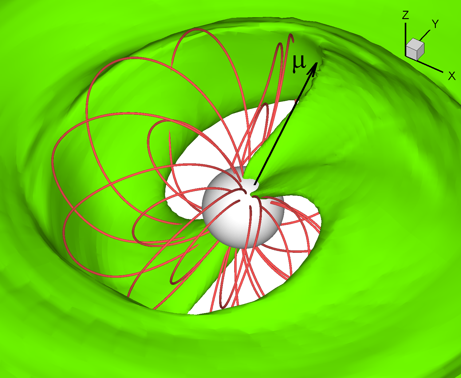
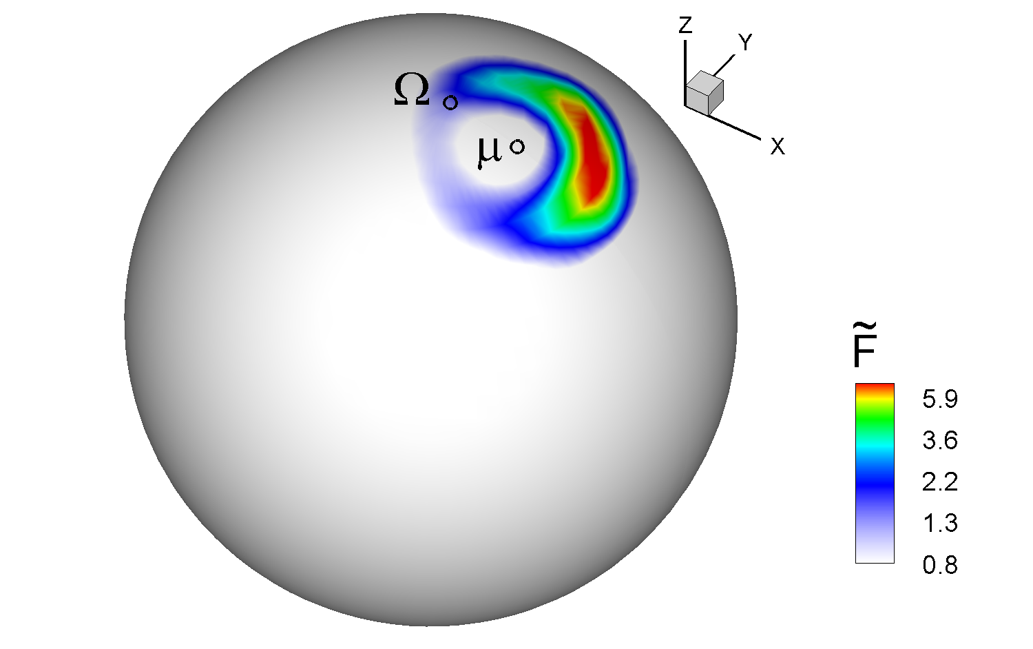
Fig. 1 (left panel) shows an example of funnel streams obtained in a typical 3D MHD simulation run. The right panel shows the energy flux distribution at the surface of the star (the hot spot). One can see that the spot has the shape of an arc, and the center of the spot (the highest energy flux) is off-set from the magnetic pole. The center of the spot is also off-set from the $\mu-\Omega$ plane, because the inner disc rotates faster than the magnetosphere, and both the funnel stream and the spot are shifted. In this paper, we provide an analytical formula for the shapes and positions of such spots.

3 Analytical Formula for the Spots

For relatively small misalignment angles, $\Theta\lesssim 30^{\circ}$, the position and shape of the spots can be approximated by analytical formula. Namely, each antipodal spot can be well approximated as a circular arc centered at the magnetic pole, with a gaussian flux distribution centered some distance away from the magnetic pole, as follows (see Fig. 2, two right panels):

$$F(\theta,\phi)=F_{c}exp\left\{-\left[\left(\frac{\theta-\theta_{0}}{\theta_{1}}\right)^{2}+\left(\frac{\phi-\phi_{0}}{\phi_{1}}\right)^{2}\right]\right\}.$$ (1)

The spherical polar and azimuthal angles $\theta$ and $\phi$ are measured with respect to the magnetic axis $\mu$. The azimuthal position $\phi=0$ is defined by the $\mu-\Omega$ plane. The spot is described by the following parameters:

• The polar and azimuthal position of the spot $(\theta_{0},\phi_{0})$.

• The polar and azimuthal width of the spot $(\theta_{1},\phi_{1})$, which are determined to be a half-width of the gaussian in the polar and azimuthal directions. The half-width is defined as the distance from the center of the spot, to the radius at which the emitted flux is 1/e times smaller than at the spot center.

• The flux emitted from the center of the spot, $F_{c}$.

We then apply a least-squares fit of this expression (given by Eq. 1) to the spots obtained from the MHD simulations. Fig. 2 compares the northern hot spot from the simulation, where misalignment angle $\Theta=10^{\circ}$ (left panel), with the fitted spot (right two panels). The fitted spot agrees well with the simulation. This procedure, when applied to the spots obtained at different parameters, shows that the rms error of the approximation is usually a few per cent.

Equation 1 gives the flux distribution for the northern hot spot. The southern hot spot is generally identical to the northern one for a dipole field, so that parameters describing it are simply $(\pi-\theta_{0},\pi+\phi_{0})$ and ($\theta_{1},\phi_{1})$. When using Eq. 1 with these parameters, care must be taken to ensure that ${|\phi-\phi_{0}|\leq\pi}$ (by adding integral multiples of $\pi$ to $\phi$) for northern spots and $|\phi-(\pi+\phi_{0})|\leq\pi$ for southern spots.

4 Dependence of spot parameters on parameters of the star

We performed a large set of 3D MHD numerical simulations at different misalignment angles of the dipole moment $\Theta$, periods of the star $P_{\star}$ and its magnetic moment $\widetilde{\mu}$. The disc is the same in all simulation runs. Our simulations and analysis show that the location and shape of the spots are determined by the following parameters:

1. Misalignment angle $\Theta$. We varied this parameter from very small values up to relatively large values: $\Theta=2^{\circ},5^{\circ},10^{\circ},20^{\circ},30^{\circ}$.

2. Magnetospheric radius $r_{m}$, normalized by stellar radius $r_{m}/R_{\star}$. The magnetospheric radius can be determined in several ways. For example, an equality of matter and magnetic stresses, $\beta_{1}=(p+\rho v_{\phi}^{2})/(B^{2}/8\pi)=1$, usually corresponds to the innermost region of the disc, where the disc density decreases sharply (e.g., Romanova et al. 2011). On the other hand, the condition $\beta=8\pi p/B^{2}$ often corresponds to the region in the disc where the funnel flow begins (Bessolaz et al., 2008). Our simulations show that the condition $\beta=1$ corresponds to the radius from which matter flows along a funnel stream to the central regions of the spots. This is why we chose the condition $\beta=1$ to derive $r_{m}$. We varied the size of the magnetosphere using the dimensionless magnetic moment of the star $\widetilde{\mu}$ in the range of $\widetilde{\mu}=0.5-2$, and obtained the magnetospheric radius in the range of $r_{m}/R_{\star}\approx 2.4-4.9$.

3. Dimensionless period of the star $P_{\star}$, or the ratio $r_{c}/R_{\star}$, where $r_{c}=[GM_{\star}(P_{\star}/2\pi)^{2}]^{1/3}$ is the corotation radius (here $P_{\star}$ is the dimensional period). In our model, we use either dimensionless period $P_{\star}$, or the ratio $r_{c}/R_{\star}$. We chose three periods for the star: $P_{\star}=1.8,2.4,2.8$ which correspond to $r_{c}/R_{\star}=4.2,5.1,5.3$ (see Table 1 for the conversion between dimensional and dimensionless values).

Figure 3: Left Panel: The sketch shows a star with a dipole magnetic field, the position of the inner disc $r=r_{m}$ and the polar angle $\theta_{s}$ of the spot’s position on the star. The magnetic axis $\mu$ of the dipole moment is tilted at an angle $\Theta$ about the rotational axis $\Omega$. Right Panel: Density distribution (color background) and magnetic field lines (yellow lines) in a typical simulation run ($\Theta=30^{\circ}$, $r_{c}=1.8$, $\widetilde{\mu}=1.5$, at $t=15$). Red lines show the dipole field lines at $t=0$. The external field lines are chosen such that both the yellow and the red lines start at the inner magnetospheric radius $r_{m}$, which is marked as a black circle.

Figure 4: The plots show that the polar angle $\theta_{0}$ (the angle between solid lines) is approximately the same for different parameters of the star. Top and bottom panels show cases of large ($\Theta=30^{\circ}$) and small ($\Theta=5^{\circ}$) misalignment angles. The left and right panels show cases of small ($\widetilde{\mu}=0.5$) and large ($\widetilde{\mu}=1.8$) magnetic moments of the star. Light-gray line shows The $\beta=1$ line is shown in light gray, and the yellow dots show the position of the magnetospheric radius $r_{m}$. The dipole field lines, which cross the magnetospheric radius are shown in cyan. The dashed black lines show the theoretically-predicted polar position of the spot, $\theta_{s}$ (see Eq. 3).

Figure 5: Left Panel: Dependence of $\phi_{0}$ on the magnetospheric radius $r_{m}/R_{\star}$ for different periods of the star $P_{\star}$. The case of $\Theta=2^{\circ}$ is removed from the set because the spot changes its position, and its averaged preferred position has a large error. Right panel: Dependence of the azimuthal position of the spot $\phi_{0}$ on the ratio of magnetopsheric to corotation radius $r_{m}/r_{c}$, taken for all simulation runs.

For each simulation run, we chose an interval of time where the accretion rate is approximately constant. We derived an averaged spot using several moments in time from this interval, then approximated the observed spot (energy flux distribution) with Eq. 1, and derived best-fit parameters $(\theta_{0},\phi_{0})$, $(\theta_{1},\phi_{1})$ and $\overline{F}_{c}$. Table 3 lists these parameters for different values of $\Theta$, $r_{m}/R_{\star}$, and $P_{\star}$ ($r_{c}/R_{\star}$). Figures 10, 11 and 12 show each of the five parameters of the spot for all simulation runs (symbols) for different misalignment angles $\Theta$ (different colors) and different periods of the star $P_{\star}$ (different symbols). Below, we discuss each parameter and derive useful dependencies.

4.1 Polar position of the spot, $\theta_{0}$

We derive the polar position of the spot using two methods: (1) simple analytical approach for a pure dipole field, and (2) numerical simulations.

4.1.1 Polar position of the spot derived from the dipole model

One of the parameters – the polar position of the spot, $\theta_{0}$, – can be derived analytically.

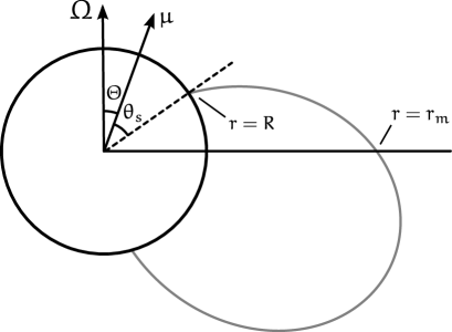
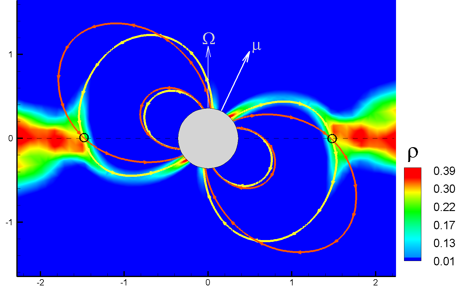
Fig. 3 (left panel) shows a schematic view of a star with a dipole field tilted at angle $\Theta$. The dipole field line which crosses the inner disc radius $r=r_{m}$ is shown. This line also shows the expected position of the spot. The dipole field lines obey the relation $r/\sin^{2}\theta=$ constant, where $\theta$ is measured from the magnetic axis. For simplicity, let us assume that the center of the spot is in the $\mu-\Omega$ plane.

Referring to Fig. 3, we have

$$\cfrac{r_{m}}{\sin^{2}\left(\cfrac{\pi}{2}-\Theta\right)}=\frac{R_{\star}}{\sin^{2}\theta_{s}},$$ (2)

which gives us the location of the spot, $\theta_{s}$, as

$$\theta_{s}=\sin^{-1}\left(\sqrt{\frac{R_{\star}}{r_{m}}}\cos\Theta\right).$$ (3)

In this idealized model, the derived angle $\theta_{s}$ shows the approximate position of the spot in the polar direction, $\theta_{0}\approx\theta_{s}$. The position of the spot depends on truncation radius $r_{m}/R_{\star}$ and misalignment angle $\Theta$.

This could be a useful approach in finding the polar position of the spots. However, numerical simulations show that the polar position is different from that derived analytically, because the magnetic field is compressed by the disc. Compression changes the shape of the field lines, affecting the position of the spots on the star.

4.1.2 Polar position of the spots derived from numerical simulations

Table 3 and Fig. 10 (left panel) show values of $\theta_{0}$ for all simulation runs. It can be seen that the polar position varies within a narrow range of angles, $16^{\circ}\lesssim\theta_{0}\lesssim 18^{\circ}$. No any significant correlation has been found between $\theta_{0}$ and the other parameters. This result is somewhat unexpected, because according to the simple estimates performed in the previous section, larger values of $\theta_{0}$ are expected for smaller misalignment angles $\Theta$ and smaller magnetospheres (smaller $r_{m}/R_{\star}$), and vice-versa. According to Eq. 3, if we use extreme parameters of $\Theta=2^{\circ}$ (the smallest misalignment angle) and $r_{m}/R_{\star}=2.4$ (the smallest magnetosphere), then we expect the largest angle to be $\theta_{0}=40.2^{\circ}$. For $\Theta=30^{\circ}$ and the largest magnetosphere, $r_{m}/R_{\star}=4.9$, we expect the smallest angle to be $\theta_{0}=23^{\circ}$. Both angles are larger than the angles obtained in our numerical simulations.

To understand this phenomenon, we compared the shapes of the magnetospheres obtained in our simulations with the shape of the dipole magnetosphere. An example of such a comparison is shown in Fig. 3 (right panel). Within the inner magnetosphere, the field lines of the simulated magnetosphere (yellow lines) depart only slightly from the dipole field line (shown in red). However, in the outer magnetosphere, the field lines of the modeled magnetosphere strongly depart from the dipole field lines. Matter flowing along the compressed field line forms a spot closer to the magnetic pole (at smaller $\theta_{0}$), compared with the theoretically-predicted position of the spot in case of a dipole field.

Fig. 3 also shows the position of the magnetospheric radius $r_{m}$, where the $\beta=1$ line crosses the equatorial plane (see two black circles). It can be seen that the field lines which start at $r_{m}$ connect the disc with the central parts of the spots.

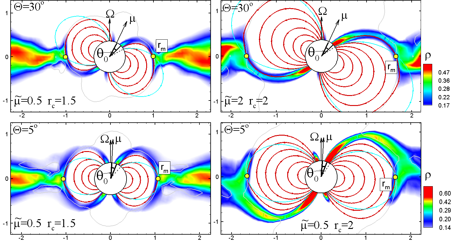
We also plot slices of density distribution in several cases with “extreme” parameters. Namely, we choose those simulation runs where parameters $\Theta$ and $r_{m}/R_{\star}$ are very large or very small. Thus, according to Eq. 3, the spots are expected to be at different polar positions $\theta_{s}$. Fig. 4 shows that in spite of the difference in parameters, the polar position of the spot $\theta_{0}$ is approximately the same and corresponds to the narrow range of values observed in Fig. 10. This can be explained by the fact that in cases of a large magnetosphere compression is not very strong, but is sufficient enough to shift the spot position towards the magnetic pole and yield a value of $\theta_{0}$ which is different from that predicted theoretically in the case of a dipole field. In cases of small magnetospheres, theoretically-predicted angle $\theta_{s}$ is larger than in cases of a large magnetosphere. However, compression of the magnetosphere is stronger, and the spot has a stronger shift towards the magnetic pole, compared with cases of a large magnetosphere. This effect leads to similar angles $\theta_{0}$ in our simulation set. It is clear that at even smaller (than in our set) magnetospheres, the theoretical dependence will not work, due to an even stronger compression of the magnetosphere. However, the formula may be applicable at very large $r_{m}/R_{\star}$, where compression is expected to be weaker.

4.2 Azimuthal position of the spot, $\phi_{0}$

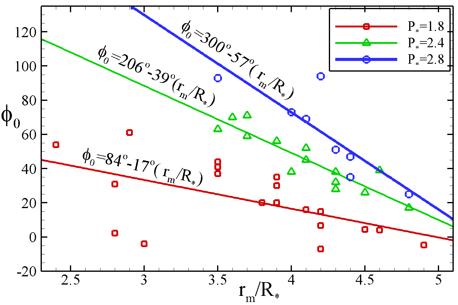
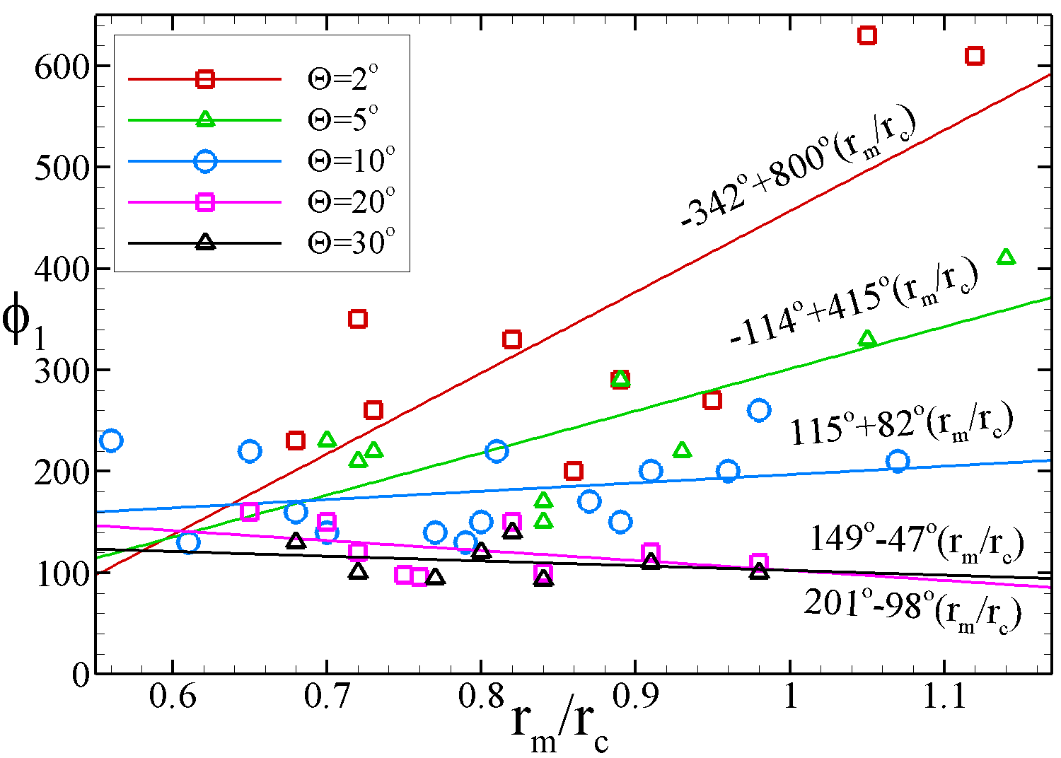
Figure 10 (right panel) shows the azimuthal position of the spots for all simulation runs. The figure shows a wide range of angles $\phi_{0}$. We noticed that some correlation can be seen between groups of runs with the same period of the star $P_{\star}$ (which are marked with the same symbol in the figure). To better demonstrate this apparent correlation, we divided all data into three groups corresponding to three periods of the star, and obtained much clearer dependencies of $\phi_{0}$ on $r_{m}/R_{\star}$. The list-square approximation shows linear correlations:

$$\phi_{0}=84^{\circ}-17^{\circ}\frac{r_{m}}{R_{\star}},~{}~{}~{}for~{}~{}~{}P_{\star}=1.8~{}~{}\left(\frac{r_{c}}{R_{\star}}=4.3\right)$$ (4)

$$\phi_{0}=206^{\circ}-39^{\circ}\frac{r_{m}}{R_{\star}},~{}~{}~{}for~{}~{}~{}P_{\star}=2.4~{}~{}\left(\frac{r_{c}}{R_{\star}}=5.1\right)$$ (5)

$$\phi_{0}=300^{\circ}-57^{\circ}\frac{r_{m}}{R_{\star}},~{}~{}~{}for~{}~{}~{}P_{\star}=2.8~{}~{}\left(\frac{r_{c}}{R_{\star}}=5.7\right)$$ (6)

It can be seen that angle $\phi_{0}$ varies more rapidly in the cases of a slower- rotating star ($P_{\star}=2.8$), and more slowly in cases of a more rapidly-rotating star ($P_{\star}=1.8$).

These dependencies can be interpreted as an azimuthal phase-shift that varies with accretion rate: smaller values of $r_{m}/R_{\star}$ correspond to higher accretion rates and stronger shifts $\phi_{0}$.

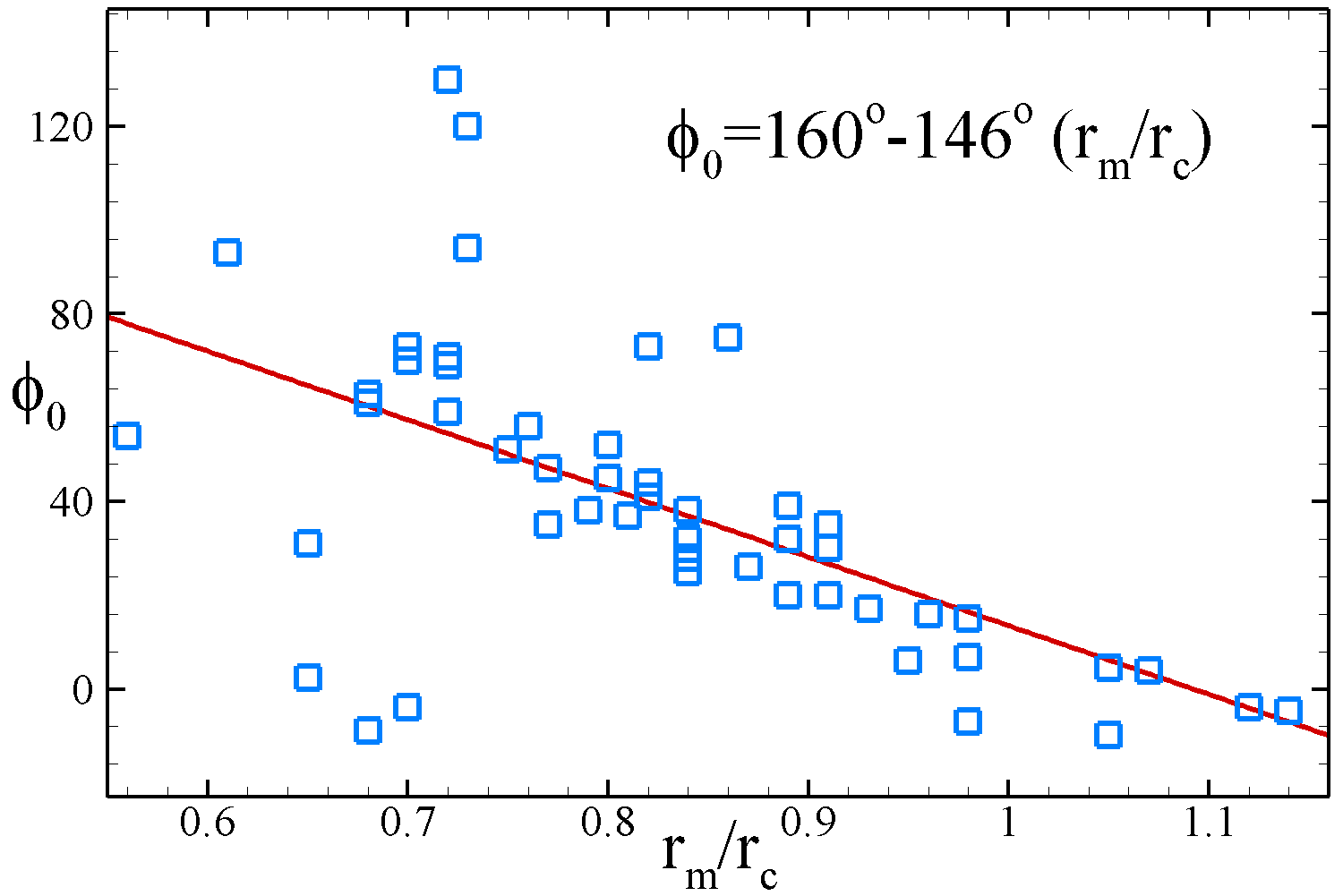
The azimuthal position of the spot depends on the relative velocity of the inner disc with respect to the magnetosphere. Hence, the dependence of $\phi_{0}$ on the ratio $r_{m}/r_{c}$ is expected. In this case, we were able to obtain a unique correlation for all simulation runs. Fig. 5 (right panel) shows this correlation. The least-square fit shows a linear dependence:

$$\phi_{0}=160^{\circ}-146^{\circ}\frac{r_{m}}{r_{c}}.$$ (7)

Therefore, if a value of $r_{m}/r_{c}$ is known, then the approximate azimuthal position of the spot is known as well.

Fig. 6 demonstrates how the spot position $\phi_{0}$ varies with $r_{m}/R_{\star}$ (which can be interpreted as variation of the accretion rate): angle $\phi_{0}$ increases when $r_{m}/R_{\star}$ decreases.

We should note that in the case of very small misalignment angle, $\Theta=2^{\circ}$, the spot changes its position rapidly, making entire $2\pi$ cycle around the magnetic pole. Hence, the azimuthal position of the spot has a large error. This is why we excluded the case of $\Theta=2^{\circ}$ from the left panel of Fig. 5.

Figure 6: The plot demonstrates different azimuthal positions $\phi_{0}$ of the spots at different magnetospheric radii $r_{m}/R_{\star}$. The spot shifts in the azimuthal direction when $r_{m}/R_{\star}$ decreases. The colored background shows the energy flux, which varies from the minimum value $F_{\rm min}=0.5$ (dark cyan color in all panels) to the maximum value $F_{\rm max}$ (red color), which is 5.8, 4.8, 3.2 and 1.9, from left to right.

4.3 Polar width of the spot, $\theta_{1}$

Figure 11 (left panel) shows that the polar width of the spots varies within a relatively narrow interval, $7^{\circ}\lesssim\theta_{1}\lesssim 10^{\circ}$, and is $\theta_{1}=7^{\circ}-8^{\circ}$ for most models. In a few cases, it is larger: $\theta_{1}=9^{\circ}$, and $\theta=10^{\circ}$ in one simulation run. There is a weak correlation between $\theta_{1}$ and $r_{m}/R_{\star}$, with $\theta_{1}$ being smaller in the cases of larger $r_{m}/R_{\star}$.

4.4 Azimuthal width of the spot, $\phi_{1}$

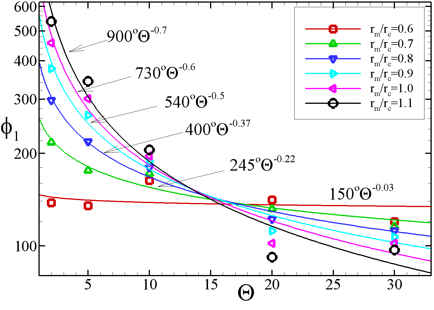
Figure 11 (right panel) shows the azimuthal width of the spots $\phi_{1}$ for all simulation runs. This parameter is also scattered significantly, like $\phi_{0}$. However, some ordered variation can be seen if we consider the subsets of runs with the same misalignment angle $\Theta$ (marked by different colors). The points with a large $\Theta$ are located at the bottom part of the plot, where $\phi_{1}\approx 100^{\circ}$ and the spots have the shape of an arc. The points with smallest $\Theta$ are located towards larger $\phi_{1}$, and have the shape of a ring.

Taking into account this (expected) dependence of $\phi_{1}$ on $\Theta$, we separate all the runs into subsets with a different $\Theta$. We notice that the correlations become stronger when we plot $\phi_{1}$ as a function of $r_{m}/r_{c}$. Fig. 7 (left panel) shows subsets of data for each $\Theta$ and a linear approximation for each subset. At large misalignment angles, $\Theta=20^{\circ}-30^{\circ}$, the azimuthal width does not vary much with $r_{m}/r_{c}$, and $\phi_{1}\approx 90^{\circ}-100^{\circ}$. However, $\phi_{1}$ strongly increases with $r_{m}/r_{c}$ for small $\Theta$. The lines which approximate sets of data have different slopes, and thus, the dependencies on $\Theta$ are different. To derive these dependencies, we choose several values of $r_{m}/r_{c}$ and take the values of $\phi_{1}$ that correspond to lines at different $\Theta$. We plot these values in Fig. 7 (right panel) and also obtain the following dependencies:

$$\phi_{1}=150^{\circ}\Theta^{-0.03},~{}~{}~{}for~{}~{}~{}r_{m}/r_{c}=0.6~{},$$ (8)

$$\phi_{1}=400^{\circ}\Theta^{-0.37},~{}~{}~{}for~{}~{}~{}r_{m}/r_{c}=0.8~{},$$ (9)

$$\phi_{1}=730^{\circ}\Theta^{-0.60},~{}~{}~{}for~{}~{}~{}r_{m}/r_{c}=1.0~{}.$$ (10)

The Figure and Eqs. 8-10 show that for $\Theta\gtrsim 15^{\circ}$, the width of the spots is relatively small for all values of $r_{m}/r_{c}$. However, for $\Theta\lesssim 15^{\circ}$, the shape varies from an arc for smaller $r_{m}/r_{c}$ to a ring for larger $r_{m}/r_{c}$. For a star with the same corotation radius $r_{c}$, larger/smaller values of $r_{m}/r_{c}$ correspond to a smaller/larger accretion rate.

Fig. 8 demonstrates the shape of the spots in the case of the same magnetic moment $\widetilde{\mu}$ and period $P_{\star}$ of the star (approximately the same value of $r_{m}/r_{c}$), but a different misalignment angle of the dipole $\Theta$. As we can see, the shapes of the spots vary from a ring (at small $\Theta$) to an arc (at large $\Theta$).

Figure 7: Left Panel: Dependence of the azimuthal width of the spot $\phi_{1}$ on the ratio of magnetic to corotation radius $r_{m}/r_{c}$ for different misalignment angles $\Theta$. Right Panel: Dependence of $\phi_{1}$ on the misalignment angle of the dipole moment $\Theta$ for different $r_{m}/r_{c}$.

Figure 8: Shapes of the spots in cases of different $\Theta$. The colored background shows the energy flux distribution. The black lines indicate the boundary where the energy flux is $e$ times smaller than the maximum flux. Other parameters are: $\widetilde{\mu}=1$, $r_{c}=1.8$, and are the same in all cases. The energy levels vary from the minimum value of $F_{\rm min}=0.5$ (light-cyan color), which is the same in all cases, to the maximum value of $F_{\rm max}$ (red color), which is $2.1$ in the three left panels, and is $3.0$ and $3.8$ in the 4th and 5th panels, respectively.

4.5 Energy flux in the center of the spots, $F_{c}$

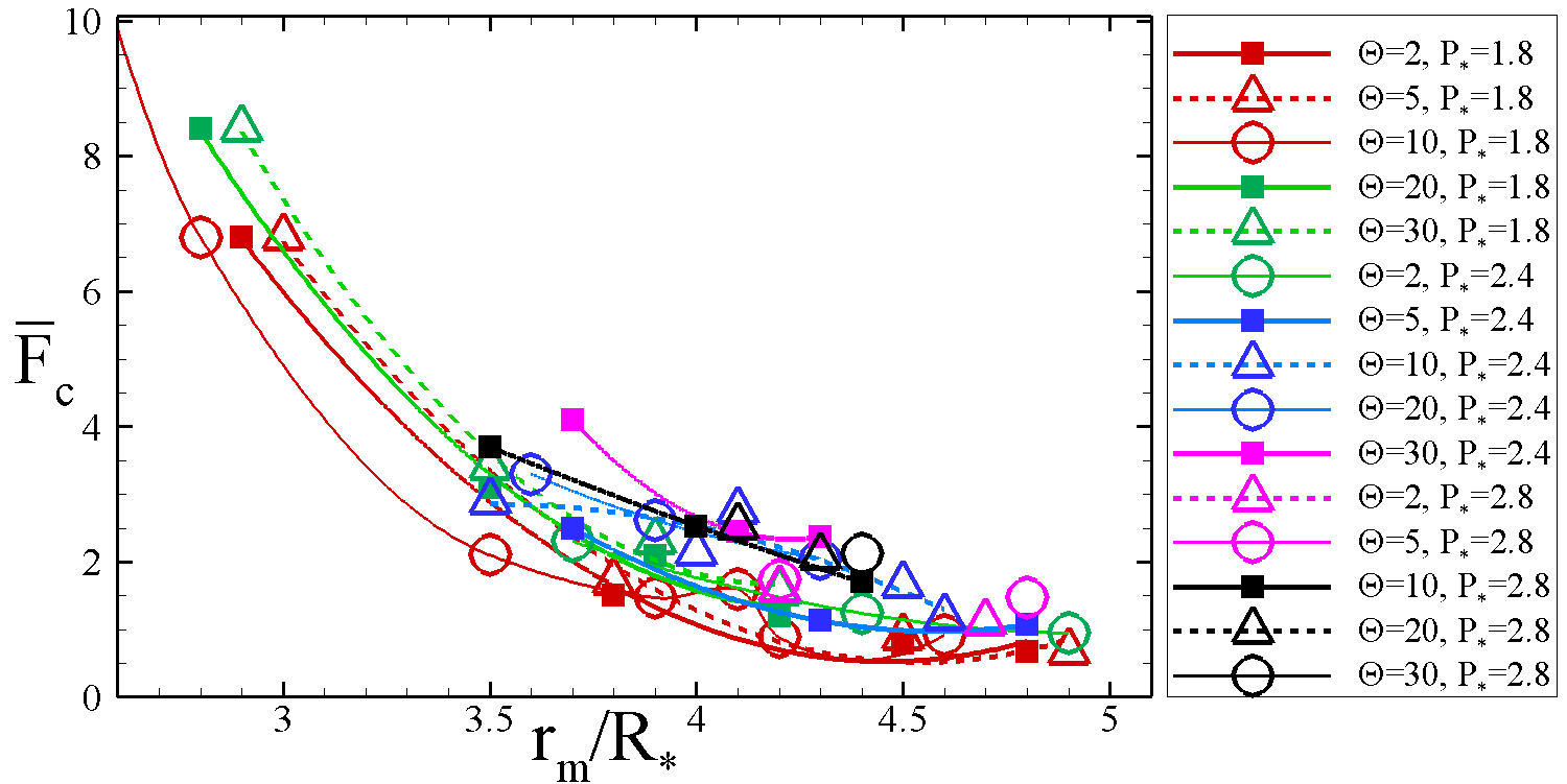
From our simulations and fits of the observed spots with Eq. 1, we obtain the maximum energy flux in the center of the spot $\widetilde{F}_{c}$ (in dimensionless units). The dimensional flux $F_{c}$, which is used in Eq. 1, can be derived from Eq. 17. It can be seen that the main dimensionless variable in Eq. 17 is the ratio $\overline{F}_{c}=\widetilde{F_{c}}/\widetilde{\mu}^{2}$. This is why we put this variable into the Table 3 and use it in Fig. 12.

Fig. 12 shows that the values of $\overline{F}_{c}$ are mainly confined to the interval $0.5\lesssim\overline{F}_{c}\lesssim 4$. It is larger, $\overline{F}_{c}\approx 6.5-8.5$, in a few points corresponding to a smaller magnetosphere, $r_{m}/R_{\star}\approx 2.8-3.2$. The fluxes are about two times smaller in cases of a small $\Theta$ (see red line in Fig. 12).

$P_{\star}$ (dim)	$r_{c}$	$r_{c}/R_{\star}$	$P_{\star}$ (CTTSs)	$P_{\star}$ (White dwarfs)	$P_{\star}$ (Neutron stars)
1.8	1.5	4.3	3.2 days	52 s	4.0 ms
2.4	1.8	5.1	4.3 days	70 s	5.3 ms
2.8	2.0	5.7	5.0 days	81 s	6.2 ms

Table 1: From left to right: dimensionless period of the star $P_{\star}$, dimensionless corotation radius $r_{c}$; corotation radius normalized to stellar radius, $r_{c}/R_{\star}$; dimensional period of the star $P_{\star}$, for different types of stars.

5 Magnetospheric radius

Magnetospheric radius $r_{m}$ (which corresponds to the boundary between the magnetosphere and the disc) is often derived from the condition that it is proportional to the Alfvén radius $r_{A}^{0}$, derived for spherical accretion under the assumption that the magnetic pressure in the magnetosphere equals to the ram pressure of free-falling matter (e.g., Lamb et al. 1973):

$$r_{m}=k_{A}r_{A}^{0}~{},~{}~{}~{}~{}~{}~{}r_{A}^{0}=\left(\frac{\mu^{4}}{2GM_{\star}\dot{M}^{2}}\right)^{1/7}~{},$$ (11)

where $k_{A}$ is the dimensionless coefficient of the order of unity. This formula has been tested a few times. In these tests, the inner disc radius has been derived in two different ways. First, it has been derived from the simulations using conditions $\beta=1$ or $\beta_{1}=1$. Second, it has been derived using formula 11 for $r_{A}^{0}$, where values such as $\mu$ and $\dot{M}$ were taken from the simulations. Long et al. (2005) performed such comparisons in three models with slightly different parameters $\mu$ and the condition $\beta_{1}=1$, and obtained an average approximate value of $k_{A}\approx 0.5$. Bessolaz et al. (2008) used a variety of definitions for the inner disc radius, such as $\beta=1$ and $\beta_{1}=1$, and obtained $k_{A}\approx 0.4$ in the case of the $\beta=1$ condition (see also Zanni & Ferreira 2013). However, none of this work studied the dependence of $r_{m}$ on $\mu$ or $\dot{M}$.

We have a sufficiently large set of simulations, so these dependencies can be tested here. As the first step, we take the formula for the Alfvén radius (Eq. 11), substitute in our dimensional units (see Sec. A), and derive the magnetospheric radius in a dimensionless form:

$$\frac{r_{m}}{R_{\star}}=\frac{k_{A}}{0.35}\bigg{(}\frac{\widetilde{\mu}^{2}}{\widetilde{\dot{M}}}\bigg{)}^{2/7}~{}.$$ (12)

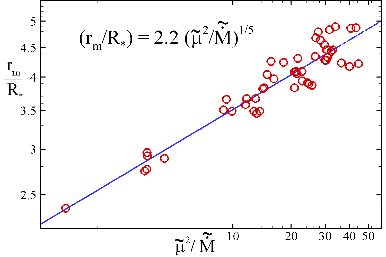
We can test this formula in our simulations, where the dimensionless magnetic moment $\widetilde{\mu}$ is the main initial parameter in each simulation run, and the dimensionless accretion rate $\widetilde{\dot{M}}$ is the output from each simulation run. We also derived the ratio $r_{m}/R_{\star}$ from the condition that $\beta=1$ in each simulation run. Fig. 9 shows the resulting dependence of $r_{m}/R_{\star}$ on ${\widetilde{\mu}^{2}}/{\widetilde{\dot{M}}}$. The dependence is well-approximated by the power law in the following form:

$$\frac{r_{m}}{R_{\star}}\approx 2.2\bigg{(}\frac{\widetilde{\mu}^{2}}{\widetilde{\dot{M}}}\bigg{)}^{1/5}~{}.$$ (13)

We can see that the power obtained from the simulations, $a\approx 0.2=1/5$ is smaller than the power given by the formula for the Alfvén radius, $a=2/7\approx 0.29$. We suggest that the compression of the magnetosphere is probably responsible for different dependence of $r_{m}$ on $\widetilde{\mu}^{2}/\widetilde{\dot{M}}$. Namely, when the magnetosphere is compressed, the magnetospheric radius varies slower with magnetic moment and accretion rate.

From the comparison of equations 13 and 12 we can derive coefficient $k_{A}$, which is not a constant anymore:

$$k_{A}\approx 0.77\bigg{(}\frac{\widetilde{\mu}^{2}}{\widetilde{\dot{M}}}\bigg{)}^{-0.086}.$$ (14)

The dependence of $k_{A}$ on $\widetilde{\mu}^{2}/\widetilde{\dot{M}}$ is weak, so that for the range of $2\lesssim\widetilde{\mu}^{2}/\widetilde{\dot{M}}\lesssim 50$ used in our set, we obtain $k_{A}$ in the range of $0.55\lesssim k_{A}\lesssim 0.72$. These values of parameter $k_{A}$ are in agreement with the values derived earlier in axisymmetric simulations (e.g., Long et al. 2005).

Next, we use Eq. 13 and Eq. 16 to derive the ratio $r_{m}/R_{\star}$ through dimensional parameters:

$$\frac{r_{m}}{R_{\star}}\approx 1.06\left(\frac{\mu^{4}}{\dot{M}^{2}GM_{\star}R_{\star}^{7}}\right)^{1/10}~{}.$$ (15)

This formula can be used if the magnetic moment of the star and the other parameters are known.

We should note that the dependence derived in Eq. 13 is relevant for the magnetospheric radii $2.5\lesssim r_{m}/R_{\star}\lesssim 5$ investigated in this work. A separate analysis should be done for larger and smaller radii. We anticipate that at larger $r_{m}/R_{\star}$ compression will be less important and the power in Eq. 15 will be larger than $0.2$, while at smaller $r_{m}/R_{\star}$ compression will be more important and the power will be smaller. Special simulation runs should be performed to investigate this dependence at larger and smaller $r_{m}/R_{\star}$.

Figure 9: Normalized magnetospheric radius $r_{m}/R_{\star}$ as a function of the ratio $\widetilde{\mu}^{2}/{\widetilde{\dot{M}}}$ for all simulation runs (circles). The line shows the power fit approximation.

6 Some Practical Considerations

The above analysis shows that the shapes and positions of the spots are determined by three parameters: (1) the misalignment angle of the dipole moment $\Theta$, (2) the normalized corotation radius $r_{c}/R_{\star}$ and (3) the normalized magnetospheric radius $r_{m}/R_{\star}$. Observations of magnetized stars are usually complex, and most of the parameters of the star and the inner disc are not known, or can be estimated only approximately. Below, we discuss possible ways to derive these parameters.

• It is often the case that the period of the star $P_{\star}$ is one of the best-known parameters. If mass $M_{\star}$ and radius $R_{\star}$ of the star are known, then the dimensionless period $P_{\star}$ and the ratio $r_{c}/R_{\star}$ can be derived.

• Many evolved magnetized stars are expected to be in the rotational equilibrium state, where a star’s spin varies around the value corresponding to rotational equilibrium. In these cases, the magnetospheric radius can be derived from condition $r_{m}=kr_{c}$ (where $k\approx 1$) . If a star is not in rotational equilibrium, then this condition cannot be used.

  In another approach, if the magnetic moment of the star and the accretion rate are known, then $r_{m}$ can be calculated from the formula for the Alfvén radius derived for spherical accretion (see Eq. 11). In this paper, we perform an independent derivation of a similar formula and find that it differs from the standard formula for the Alfvén radius (see Sec. 5).

• One of the most important parameters, $\phi_{0}$, which stands for the azimuthal shift of the spot, depends only on the ratio $r_{m}/r_{c}$ (see Eq. 5). If a star is in the rotational equilibrium state, then the value $r_{m}/r_{c}\approx$ can be taken from numerical simulations. Axisymmetric simulations performed by Long et al. (2005) show that $r_{m}/r_{c}\approx 0.7-0.8$, while Zanni & Ferreira (2013) found $r_{m}/r_{c}\approx 0.6$. This ratio is smaller, when a larger amount of angular momentum flows into the corona along inflated or partially-inflated field lines. This ratio can also vary in time. Therefore, the above numbers are approximate and can be used only as estimates.

• The misalignment angle of the dipole’s magnetic moment $\Theta$, is known approximately in some cases. For example, in a few CTTSs, the magnetic field distribution on the surface of the star has been derived from polarimetric observations and then approximated with the set of tilted magnetic moments of a different order. It was found that the misalignment angle of the dipole component is usually small, $\Theta\approx 10^{\circ}-20^{\circ}$ (e.g., (Donati et al., 2008)). In some cases, the misalignment angle can be obtained from the shapes of observed light-curves and comparisons with those obtained in 3D MHD numerical simulations (Romanova et al., 2004). For example, for some probable inclination angle of $i\approx 45^{\circ}$, a nearly-symmetric light-curves with one peak per period yield a relatively small misalignment angles, $\Theta\lesssim 30^{\circ}$, while light-curves with two peaks per period yield a larger $\Theta$.

7 Conclusions and Discussion

In this work we derived a useful analytical formula (Eq. 1) that provides an approximation for arc-shaped and ring-shaped spots which form in accreting magnetized stars. Multiple 3D MHD simulation runs were performed to find the positions of the spots ($\theta_{0}$, $\phi_{0}$), their shapes ($\theta_{1}$, $\phi_{1}$) and their dependencies on the period of the star $P_{\star}$, the misalignment angle of the dipole $\Theta$, and the ratio of the magnetospheric radius to the radius of the star, $r_{m}/R_{\star}$. The main conclusions are as follows:

1. The polar positions of the spots $\theta_{0}$ vary within the narrow range of $16^{\circ}\lesssim\theta_{0}\lesssim 18^{\circ}$. These angles are different from the polar angles obtained with the simple analytical formula (see Eq. 3), where $\theta_{0}$ has larger values and varies considerably with $r_{m}/R_{\star}$ and the dipole misalignment angle $\Theta$. We noticed that in all our numerical models the external closed magnetosphere is compressed and departs significantly from the dipole shape, which leads to the misplacement of the spot.

2. The azimuthal positions of the spots $\phi_{0}$ strongly vary with the magnetospheric radius $r_{m}/R_{\star}$ (accretion rate). They increase, when $r_{m}$ decreases. For the same interval of $r_{m}/R_{\star}$, $\phi_{0}$ varies more rapidly for stars with larger periods.

3. An important correlation has been found for the dependence of $\phi_{0}$ on the ratio $r_{m}/r_{c}$, which is valid for all simulation runs.

4. The polar widths of the spots $\theta_{1}$ vary within the narrow interval of $7^{\circ}\lesssim\theta_{1}\lesssim 9^{\circ}$, and the majority of the spots have a width of $7^{\circ}-8^{\circ}$.

5. The azimuthal widths of the spots $\phi_{1}$ strongly depend on the dipole misalignment angle $\Theta$. They vary from $\phi_{1}=90^{\circ}-100^{\circ}$ for $\Theta=30^{\circ}$ (arc-shaped spots) to $\phi_{1}\approx 600^{\circ}$ for $\Theta=2^{\circ}$ (ring-shaped spots).

6. We also used our data to check the formula for the Alfvén radius, where the main dependence is $r_{m}\sim(\mu^{2}/{\dot{M}})^{2/7}$. We found that the dependence is more gradual, $r_{m}\sim(\mu^{2}/{\dot{M}})^{1/5}$, which can be explained by the compression of the magnetosphere by the disc matter and by the non-dipole shape of the magnetic field lines of the external magnetosphere.

Once these parameters are known, the analytical formula given by Eq. 1 can be used to model the energy flux distribution in the spot. The light-curves can be calculated using a separate numerical program. In this program, the radiation model, the anisotropy of the radiation, and the inclination angle of the system can be taken into account. For neutron stars, this code should take into account relativistic light-bending, Doppler-shift and other relativistic effects (see, e.g., Kulkarni & Romanova 2005).

Variation of the azimuthal position of the spot $\phi_{0}$ with accretion rate is particularly important for observations. For example, in millisecond pulsars, it may lead to phase-shifts in light-curves (Patruno et al., 2009) and timing noise (e.g., Poutanen et al. 2009). In CTTSs, it can lead to the phenomenon of a drifting period, where the period derived at different times of observation, is different, and therefore, it varies with time (e.g., Rucinski et al. 2008).

Here, we present results for a relatively narrow interval of the ratio $0.6\lesssim r_{m}/r_{c}\lesssim 1.1$, which corresponds to ordered accretion through two funnel streams. The smallest values correspond to a boundary between stable and unstable regimes of accretion , where at $r_{m}/r_{c}\lesssim 0.6$ accretion proceeds in the equatorial plane through the magnetic Rayleigh-Taylor instability. The largest value, $r_{m}/r_{c}\approx 1.1$, corresponds to the propeller regime, in which the funnel accretion is forbidden by the centrifugal barrier (e.g., Illarionov & Sunyaev 1975; Lovelace et al. 1999).

Of course, the analytical formula (Eq. 1) describing the shape of the spot can be applied only in the cases where the magnetic field of the star has a strong dipolar component. In the case of a more complex field, the higher order component of the field may govern the funnel flow near the star, and the shapes of the spots will be determined by higher order multipoles of the field (e.g., Long et al. 2011; Romanova et al. 2011). This case should be investigated separately.

Acknowledgments

Authors thank Alisa Blinova for help and Alexander Koldoba for an earlier-developed ‘cubed sphere’ code. Resources supporting this work were provided by the NASA High-End Computing (HEC) Program through the NASA Advanced Supercomputing (NAS) Division at Ames Research Center and the NASA Center for Computational Sciences (NCCS) at Goddard Space Flight Center. The research was supported by NASA grants NNX10AF63G, NNX11AF33G and NSF grant AST-1008636.

Appendix A Reference Values

	CTTSs	White dwarfs	Neutron stars
$M_{\star}(M_{\odot})$	0.8	1	1.4
$R_{\star}$	$2R_{\odot}$	5000 km	10 km
$B_{\star}$ (G)	$10^{3}$	$10^{6}$	$10^{9}$
$\mu$	1	1	1
$R_{0}$ (cm)	$4\times 10^{11}$	$1.4\times 10^{9}$	$2.9\times 10^{6}$
$P_{0}$	1.8 days	29 s	2.2 ms
$B_{0}$ (G)	43	$4.3\times 10^{4}$	$4.3\times 10^{7}$
$\dot{M}_{0}$ ($M_{\odot}$yr-1)	$2.8\times 10^{-7}$	$1.9\times 10^{-7}$	$2.9\times 10^{-8}$
$F_{0}$ (erg s-1cm-2)	$3\times 10^{10}$	$5.6\times 10^{17}$	$1.5\times 10^{25}$

Table 2: Sample reference values of the dynamical quantities used in our simulations in the case where dimensionless magnetic moment $\widetilde{\mu}=1$. Note that parameters $\rho_{0}$, $B_{0}$, $\dot{M}_{0}$ and $F_{0}$ depend on $\widetilde{\mu}$ (see Sec. A).

Our simulations are done using dimensionless variables (denoted here by a tilde), obtained by dividing the dimensional variables by reference values. The reference values are determined as follows: We choose fiducial values for stellar mass $M_{\star}$, radius $R_{\star}$ and equatorial surface magnetic field $B_{\star}$; the reference values of all other dynamical quantities are then obtained from these fiducial values. The unit of distance is chosen to be $R_{0}=R_{\star}/0.35$. The reference velocity is the Keplerian velocity at $R_{0}$, $v_{0}=(GM_{\star}/R_{0})^{1/2}$, and $\omega_{0}=v_{0}/R_{0}$ is the reference angular velocity. The reference time is the Keplerian rotation period at $R_{0}$, $P_{0}=2\pi R_{0}/v_{0}$.

The reference magnetic moment $\mu_{0}$ = $\mu/\widetilde{\mu}$, where $\widetilde{\mu}$ is the dimensionless magnetic moment of the star. The reference magnetic field is $B_{0}=\mu_{0}/R_{0}^{3}$. The reference density is $\rho_{0}=B_{0}^{2}/v_{0}^{2}$. The reference accretion rate is $\dot{M}_{0}=\rho_{0}v_{0}R_{0}^{2}$. Using the relationships for $\rho_{0}$, $B_{0}$ and $v_{0}$, we obtain $\dot{M}_{0}=\mu^{2}/(\widetilde{\mu}^{2}v_{0}R_{0}^{4})$. The dimensional accretion rate is $\dot{M}=\widetilde{\dot{M}}\dot{M}_{0}$, where $\widetilde{\dot{M}}$ is the dimensionless accretion rate onto the surface of the star which is obtained from the simulations. Substituting the expression for $\dot{M}_{0}$ and using $\mu=B_{\star}R_{\star}^{3}$, we get

$$\dot{M}=\left(\frac{\widetilde{\dot{M}}}{\widetilde{\mu}^{2}}\right)\frac{B_{\star}^{2}R_{\star}^{5/2}(0.35)^{7/2}}{(GM_{\star})^{1/2}}.$$ (16)

Thus, if the stellar parameters $M_{\star}$, $R_{\star}$ and $B_{\star}$ are fixed, then the accretion rate is determined by $\widetilde{\dot{M}}/\widetilde{\mu}^{2}$. Therefore, variation of parameter $\widetilde{\mu}$ can be interpreted as variation of the magnetospheric radius of the star, or it can be equally validly interpreted as a parameter that is responsible for variation of the accretion rate.

The reference energy flux is defined as $F_{0}=\rho_{0}v_{0}^{3}$. Using this formula, we get a similar conversion formula for the energy flux:

$$F=\left(\frac{\widetilde{F}}{\widetilde{\mu}^{2}}\right)\frac{B_{\star}^{2}(GM_{\star})^{1/2}(0.35)^{13/2}}{R_{\star}^{1/2}}.$$ (17)

We use a dimensionless parameter $\overline{F}_{c}={\widetilde{F_{c}}}/{\widetilde{\mu}^{2}}$ to characterize the flux in the centers of the spots.

Appendix B Parameters of Spots

Parameters of the spots for all simulation runs are given in Table 3. Simulations were done for five misalignment angles $\Theta=2^{\circ},5^{\circ},10^{\circ},20^{\circ},30^{\circ}$ and three (dimensionless) periods of the star $P_{\star}=1.8,2.4,2.8$, which correspond to normalized corotation radii of $r_{c}/R_{\star}=4.3,5.1,5.7$. In each set of runs with the same parameters $\Theta$ and $P_{\star}$, we varied the dimensionless magnetic moment of the star $\widetilde{\mu}$ and observed that the magnetospheric radius $r_{m}$ increases with $\widetilde{\mu}$. The magnetospheric radius is an important parameter because the funnel flow starts approximately at $r_{m}$. In this paper, we use the dimensionless ratio $r_{m}/R_{\star}$, so that results can be applied to different types of stars.

Table 3 shows the polar and azimuthal positions of the spots ($\theta_{0}$, $\phi_{0}$), their polar and azimuthal widths ($\theta_{1}$, $\phi_{1}$) and the ratio $\widetilde{F}_{c}/\widetilde{\mu}^{2}$, which characterizes the dimensionless energy flux in the centers of the spots. If parameters $\Theta$, $r_{c}/R_{\star}$ and $r_{m}/R_{\star}$ are known, then Table 3 provides the positions and shapes of the spots.

Figures 10, 11 and 12 show parameters of the spots for all simulation runs. Fig. 10 shows the polar and azimuthal positions of the spots. Fig. 11 shows the polar and azimuthal widths of the spots. Fig. 12 shows dimensionless energy flux in the center of the spots. A set of runs with the same $\Theta$ is marked by the same color. A set of runs with the same $P_{\star}$ is marked by the same symbols. The lines show interpolations between points corresponding to sets of runs with the same $\Theta$ and $P_{\star}$. These lines helped us derive important dependencies discussed in the paper (see Sec. 4).

Figure 10: Left panel: The polar coordinates of the spots position $\theta_{0}$ in all simulation runs as a function of the magnetospheric radius normalized to the stellar radius, $r_{m}/R_{\star}$, for different misalignment angles: $\Theta=2^{\circ}$ (red color), $\Theta=5^{\circ}$ (green color), $\Theta=10^{\circ}$ (blue color), $\Theta=20^{\circ}$ (pink color), and $\Theta=30^{\circ}$ (black color), and for different periods of the star: $P_{\star}=1.8$ (thick solid lines, squares), $P_{\star}=2.4$ (dashed lines, triangles), and $P_{\star}=2.8$ (thin solid lines, circles). The symbols show results of individual simulation runs, while the lines show interpolation between runs performed for the same parameters $\Theta$ and $P_{\star}$.

Figure 11: Width of the spots in polar ($\theta_{1}$, see left panel) and azimuthal ($\phi_{1}$, see right panel) directions as a function of the magnetospheric radius normalized to the stellar radius, $r_{m}/R_{\star}$. Symbols and lines are the same as is in Fig. 10.

$\Theta=2^{\circ}$ $P_{\star}$ $r_{m}/R_{\star}\rightarrow$ 2.9 3.7 3.8 4.2 4.4 4.5 4.7 4.8 4.9 ($r_{c}/R_{\star}$) 1.8 (4.3) $\theta_{0},\phi_{0}$ 18, -8.9 18, 32 17, -9.8 17, -3.9 $\theta_{1},\phi_{1}$ 9, 230 9, 290 8, 630 8, 610 $\overline{F}_{c}$ 1.7 1.5 1.8 2.7 2.4 (5.1) $\theta_{0},\phi_{0}$ 17, 130 16, 75 16, 6 $\theta_{1},\phi_{1}$ 8, 350 8, 200 8, 270 $\overline{F}_{c}$ 2.3 2.8 3.8 2.8 (5.7) $\theta_{0},\phi_{0}$ 16, 120 16, 73 $\theta_{1},\phi_{1}$ 8, 260 8, 330 $\overline{F}_{c}$ 3.6 4.4

$\Theta=5^{\circ}$ $P_{\star}$ $r_{m}/R_{\star}\rightarrow$ 3 3.7 3.8 4.2 4.3 4.5 4.8 4.9 ($r_{c}/R_{\star}$) 1.8 (4.3) $\theta_{0},\phi_{0}$ 18, -3.9 18, 20 17, 4.4 17, -4.6 $\theta_{1},\phi_{1}$ 9, 230 9, 290 8, 330 8, 410 $\overline{F}_{c}$ 1.7 1.7 2 2.7 2.4 (5.1) $\theta_{0},\phi_{0}$ 17, 71 17, 32 17, 17 9, 210 8, 170 8, 220 $\overline{F}_{c}$ 2.5 3.8 4.3 2.8 (5.7) $\theta_{0},\phi_{0}$ 16, 94 16, 25 $\theta_{1},\phi_{1}$ 8, 220 7, 150 $\overline{F}_{c}$ 3.9 5.9

$\Theta=10^{\circ}$ $P_{\star}$ $r_{m}/R_{\star}\rightarrow$ 2.4 2.8 3.5 3.9 4 4.1 4.2 4.4 4.5 4.6 ($r_{c}/R_{\star}$) 1.8 (4.3) $\theta_{0},\phi_{0}$ 17, 54 18, 2.3 17, 37 17, 20 18, 16 18, -7 18, 4 $\theta_{1},\phi_{1}$ 10, 230 9, 220 8, 220 8, 200 8, 200 8, 260 7, 210 $\overline{F}_{c}$ 1.3 1.7 2.1 3.3 2.5 2.7 3.7 2.4 (5.1) $\theta_{0},\phi_{0}$ 17, 63 17, 38 16, 45 17, 26 16, 39 $\theta_{1},\phi_{1}$ 8, 160 8, 130 7, 150 7, 170 7, 150 $\overline{F}_{c}$ 2.9 4.8 4.3 5.1 4.7 2.8 (5.7) $\theta_{0},\phi_{0}$ 18, 93 16, 73 16, 35 $\theta_{1},\phi_{1}$ 8, 130 8, 140 7, 140 $\overline{F}_{c}$ 3.7 5.7 6.8

$\Theta=20^{\circ}$ $P_{\star}$ $r_{m}/R_{\star}\rightarrow$ 2.8 3.5 3.6 3.9 4.1 4.2 4.3 ($r_{c}/R_{\star}$) 1.8 (4.3) $\theta_{0},\phi_{0}$ 17, 31 18, 41 17, 35 18, 6.8 $\theta_{1},\phi_{1}$ 9, 160 8, 150 8, 120 7, 110 $\overline{F}_{c}$ 2.1 3.1 4.7 4.8 2.4 (5.1) $\theta_{0},\phi_{0}$ 17, 70 17, 56 17, 28 $\theta_{1},\phi_{1}$ 8, 150 7, 96 7, 100 $\overline{F}_{c}$ 3.3 5.9 8.2 2.8 (5.7) $\theta_{0},\phi_{0}$ 17, 69 17, 51 $\theta_{1},\phi_{1}$ 7, 120 7, 98 $\overline{F}_{c}$ 5.7 8.3

$\Theta=30^{\circ}$ $P_{\star}$ $r_{m}/R_{\star}\rightarrow$ 2.9 3.5 3.7 3.9 4.1 4.2 4.3 4.4 ($r_{c}/R_{\star}$) 1.8 (4.3) $\theta_{0},\phi_{0}$ 17, 61 17, 44 16, 30 17, 15 $\theta_{1},\phi_{1}$ 9, 130 8, 140 8, 110 7, 100 $\overline{F}_{c}$ 2.1 3.4 5.2 6.2 2.4 (5.1) $\theta_{0},\phi_{0}$ 18, 59 16, 52 16, 38 $\theta_{1},\phi_{1}$ 8, 100 8, 120 7, 93 $\overline{F}_{c}$ 4.1 5.5 9.5 2.8 (5.7) $\theta_{0},\phi_{0}$ 17, 47 $\theta_{1},\phi_{1}$ 7, 94 $\overline{F}_{c}$ 8.5

Table 3: Parameters of the spots for different dipole misalignment angles $\Theta$, three periods of the star, $P=1.8,2,2.4$, and different magnetospheric radii $r_{m}/R_{\star}$. Polar and azimuthal angles ($\theta_{0}$ and $\phi_{0}$, respectively) determine the polar and azimuthal positions of the spots. Polar and azimuthal angles ($\theta_{1}$ and $\phi_{1}$, respectively) determine the size of the spots. The dimensionless function $\overline{F}_{c}=\widetilde{F}_{c}/\widetilde{\mu}^{2}$ determines the energy flux in the centers of the spots.

Figure 12: Dimensionless function $\overline{F}_{c}=\widetilde{F}_{c}/\widetilde{\mu}^{2}$ (which determines the energy flux in the centers of the spots) shown for all simulation runs. Symbols and lines are the same as is in Fig. 10.

References

- Bachetti et al. (2010) Bachetti M., Romanova M. M., Kulkarni A., Burderi L., di Salvo T., 2010, MNRAS, 403, 1193
- Bessolaz et al. (2008) Bessolaz N., Zanni C., Ferreira J., Keppens R., Bouvier J., 2008, A&A, 478, 155
- Bouvier et al. (2007) Bouvier J., Alencar S. H. P., Harries T. J., Johns-Krull C. M., Romanova M. M., 2007, in Reipurth B., Jewitt D., Keil K., eds, Protostars and Planets V Magnetospheric Accretion in Classical T Tauri Stars. pp 479–494
- Donati et al. (2008) Donati J.-F., Jardine M. M., Gregory S. G., Petit P., Paletou F., Bouvier J., Dougados C., Ménard F., Collier Cameron A., Harries T. J., Hussain G. A. J., Unruh Y., Morin J., Marsden S. C., Manset N., et al. 2008, MNRAS, 386, 1234
- Ghosh & Lamb (1979) Ghosh P., Lamb F. K., 1979, ApJ, 232, 259
- Ibragimov & Poutanen (2009) Ibragimov A., Poutanen J., 2009, MNRAS, 400, 492
- Illarionov & Sunyaev (1975) Illarionov A. F., Sunyaev R. A., 1975, A&A, 39, 185
- Koldoba et al. (2002) Koldoba A. V., Romanova M. M., Ustyugova G. V., Lovelace R. V. E., 2002, ApJ, 576, L53
- Kulkarni & Romanova (2005) Kulkarni A. K., Romanova M. M., 2005, ApJ, 633, 349
- Kulkarni & Romanova (2008) Kulkarni A. K., Romanova M. M., 2008, MNRAS, 386, 673
- Lamb et al. (2008) Lamb F. K., Boutloukos S., Van Wassenhove S., Chamberlain R. T., Lo K. H., Clare A., Yu W., Miller M. C., 2008, ArXiv e-prints
- Lamb et al. (2009) Lamb F. K., Boutloukos S., Van Wassenhove S., Chamberlain R. T., Lo K. H., Clare A., Yu W., Miller M. C., 2009, ApJ, 706, 417
- Lamb et al. (1973) Lamb F. K., Pethick C. J., Pines D., 1973, ApJ, 184, 271
- Leahy et al. (2009) Leahy D. A., Morsink S. M., Chung Y.-Y., Chou Y., 2009, ApJ, 691, 1235
- Long et al. (2011) Long M., Romanova M. M., Kulkarni A. K., Donati J.-F., 2011, MNRAS, 413, 1061
- Long et al. (2005) Long M., Romanova M. M., Lovelace R. V. E., 2005, ApJ, 634, 1214
- Lovelace et al. (1999) Lovelace R. V. E., Romanova M. M., Bisnovatyi-Kogan G. S., 1999, ApJ, 514, 368
- Novikov & Thorne (1973) Novikov I. D., Thorne K. S., 1973, in Black Holes (Les Astres Occlus) Astrophysics of black holes.. pp 343–450
- Paczyński & Wiita (1980) Paczyński B., Wiita P. J., 1980, A&A, 88, 23
- Patruno et al. (2009) Patruno A., Wijnands R., van der Klis M., 2009, ApJ, 698, L60
- Poutanen & Gierliński (2003) Poutanen J., Gierliński M., 2003, MNRAS, 343, 1301
- Poutanen et al. (2009) Poutanen J., Ibragimov A., Annala M., 2009, ApJ, 706, L129
- Powell et al. (1999) Powell K. G., Roe P. L., Linde T. J., Gombosi T. I., de Zeeuw D. L., 1999, Journal of Computational Physics, 154, 284
- Romanova et al. (2008) Romanova M. M., Kulkarni A. K., Long M., Lovelace R. V. E., 2008, in Wijnands R., ed., A Decade of Accreting Millisecond X-ray Pulsars Modeling of Disk-Star Interaction: Different Regimes of Accretion and Variability. pp 87–94
- Romanova et al. (2011) Romanova M. M., Long M., Lamb F. K., Kulkarni A. K., Donati J.-F., 2011, MNRAS, 411, 915
- Romanova et al. (2002) Romanova M. M., Ustyugova G. V., Koldoba A. V., Lovelace R. V. E., 2002, ApJ, 578, 420
- Romanova et al. (2004) Romanova M. M., Ustyugova G. V., Koldoba A. V., Lovelace R. V. E., 2004, ApJ, 610, 920
- Romanova et al. (2003) Romanova M. M., Ustyugova G. V., Koldoba A. V., Wick J. V., Lovelace R. V. E., 2003, ApJ, 595, 1009
- Rucinski et al. (2008) Rucinski S. M., Matthews J. M., Kuschnig R., Pojmański G., Rowe J., Guenther D. B., Moffat A. F. J., Sasselov D., Walker G. A. H., Weiss W. W., 2008, MNRAS, 391, 1913
- Shakura & Sunyaev (1973) Shakura N. I., Sunyaev R. A., 1973, A&A, 24, 337
- Spruit et al. (1995) Spruit H. C., Stehle R., Papaloizou J. C. B., 1995, MNRAS, 275, 1223
- Warner (1995) Warner B., 1995, Cataclysmic variable stars. Cambridge Astrophysics Series, Cambridge, New York: Cambridge University Press, —c1995
- Zanni & Ferreira (2013) Zanni C., Ferreira J., 2013, A&A, 550, A99